

Dynamical Study of Coupled Riemann Wave Equation Involving Conformable, Beta, and M-Truncated Derivatives via Two Efficient Analytical Methods

 ,
,  , , and
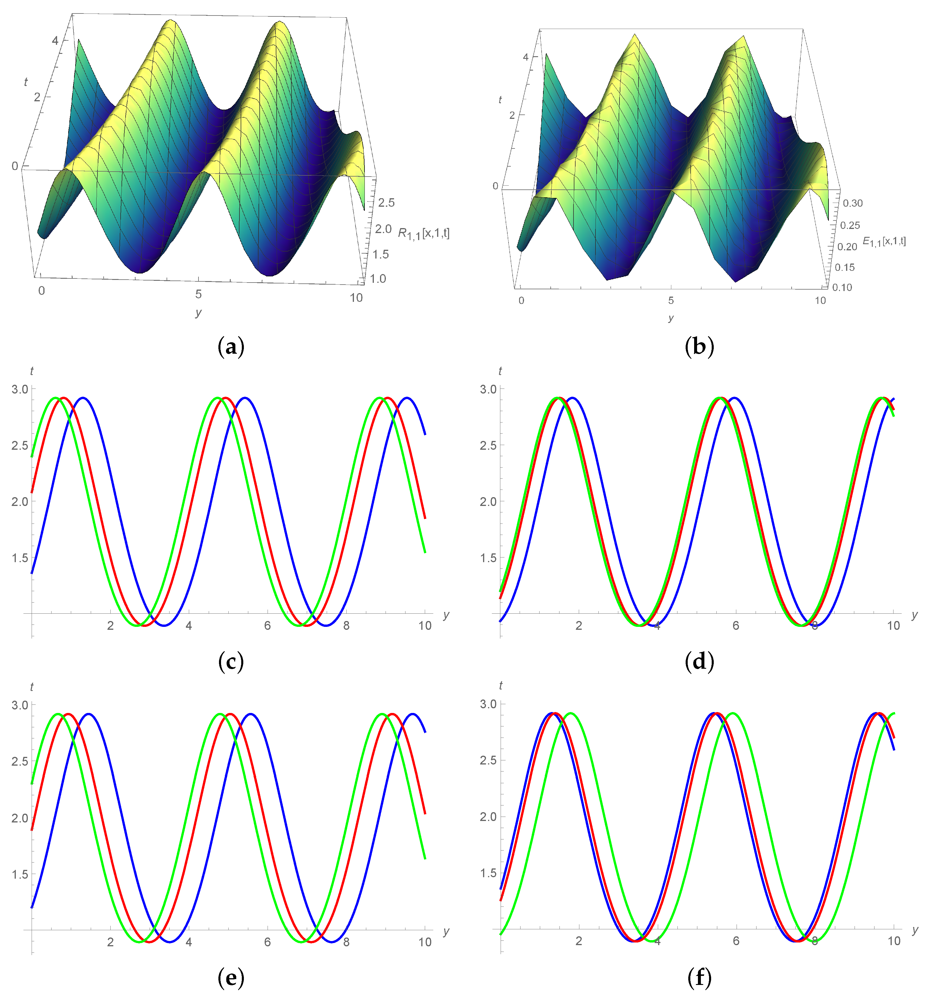
Abstract
:1. Introduction
2. Preliminaries
2.1. Beta-Derivative
- The -D is a linear operator; that is,
- This satisfies the product rule; that is,
- This obeys the quotient rule; that is,
- The -D of a constant is zero; that is,for any constant c.
2.2. M-Truncated Derivative
- 1.
- , .
- 2.
- .
- 3.
- .
- 4.
- The M-TD for a differentiable function is defined as:
2.3. Conformable Derivative
3. Mathematical Analyses of the Procedure
4. Application of Analytical Methods
4.1. Jacobi Elliptic Function Method
4.2. Modified Auxiliary Equation Method
- If , thenor
- If , thenor
- If , then
- For , the trigonometric solution is:or
- For , the hyperbolic solution is:or
- For , the trigonometric solution is:or
- For , the hyperbolic solution is:or
- For , the trigonometric solution is:or
- For , the hyperbolic solution is:or
- For , the trigonometric solution is:or
- For , the hyperbolic solution is:or
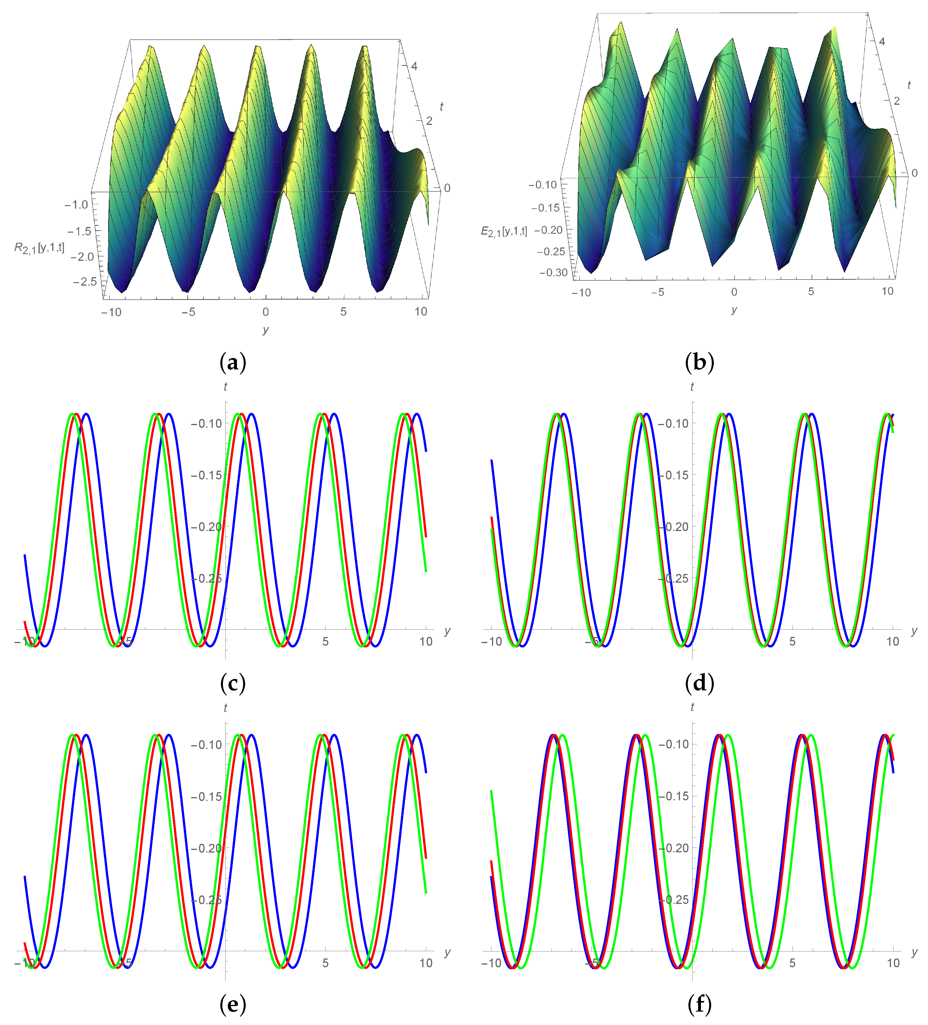
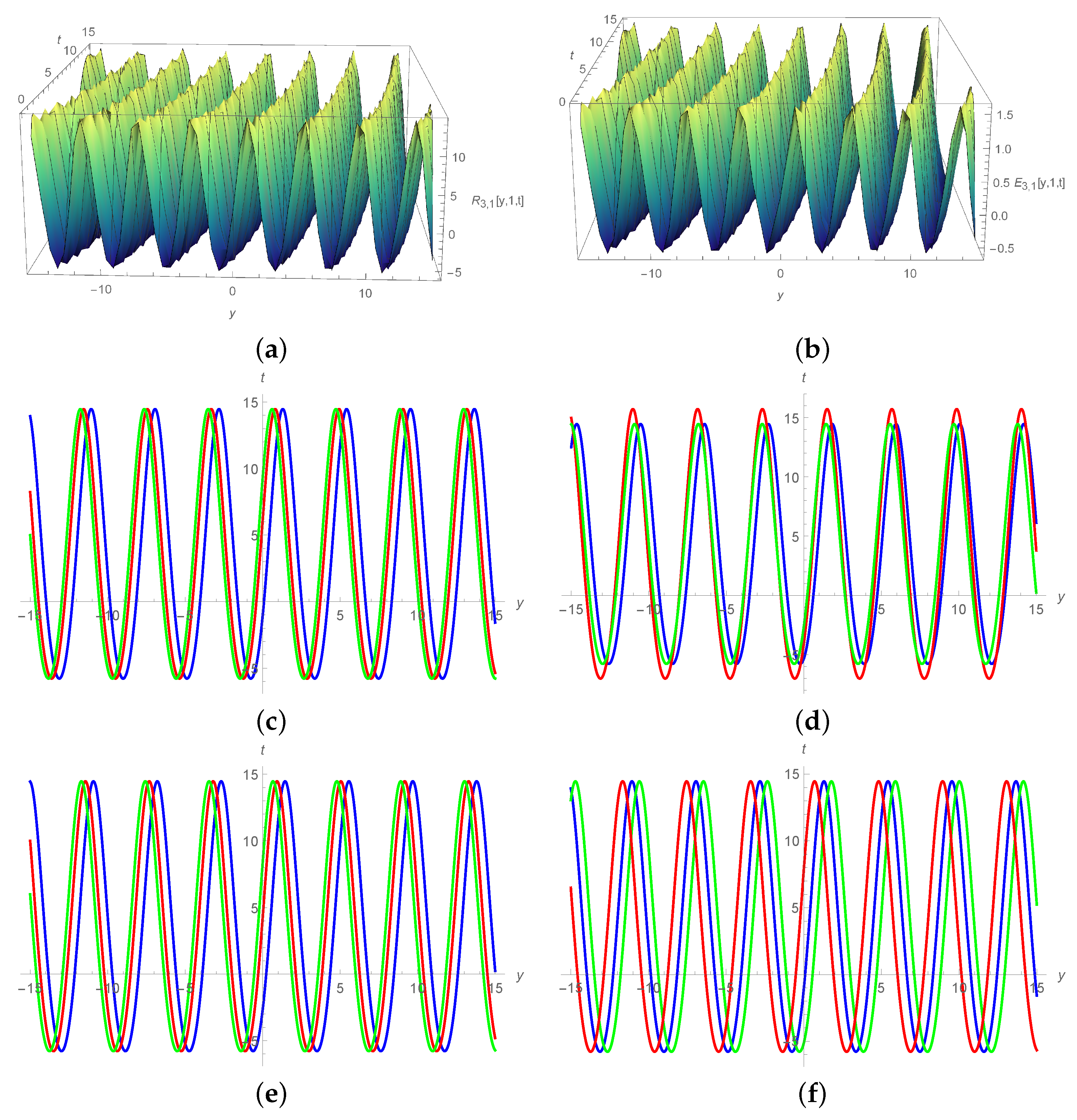
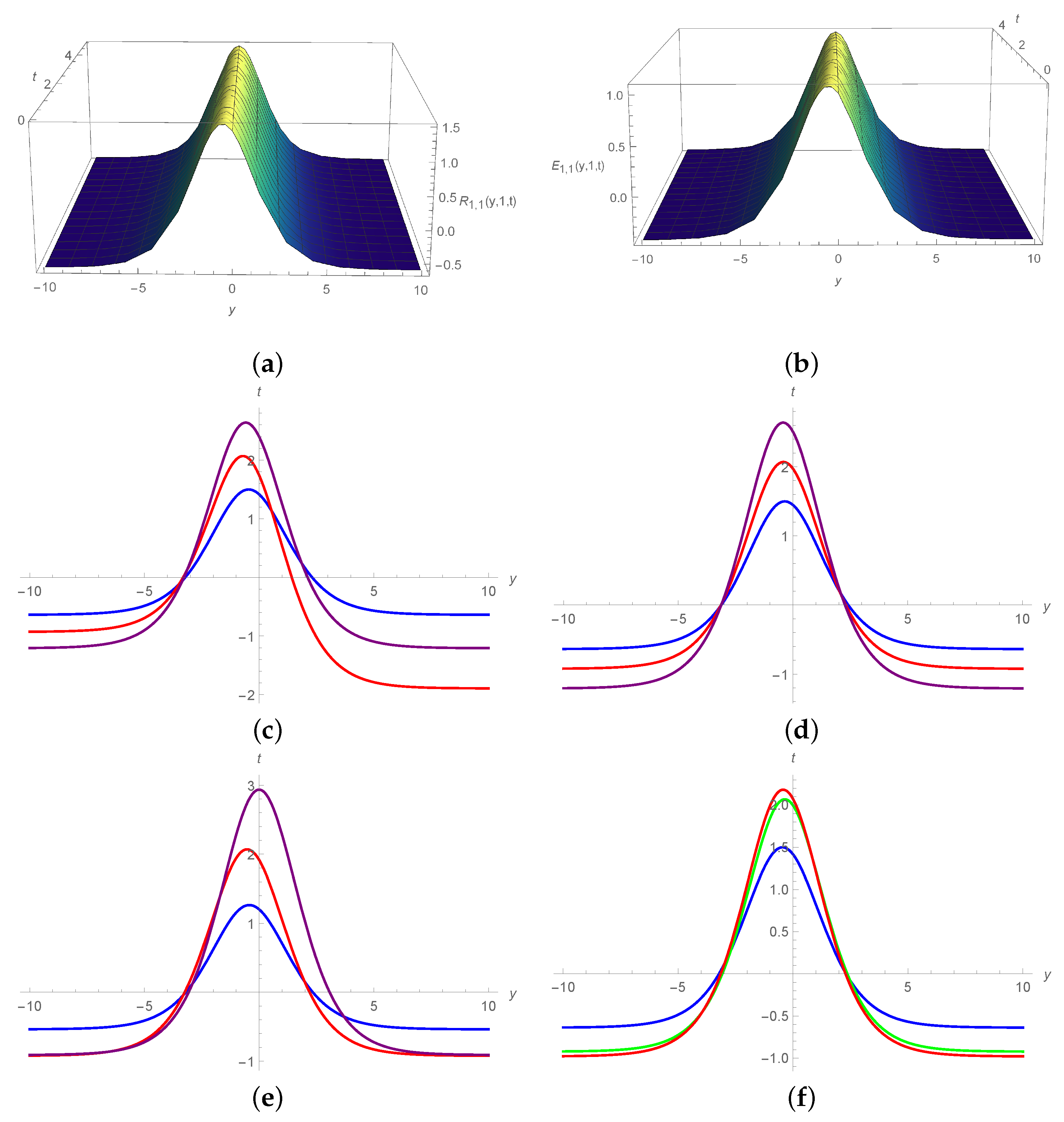
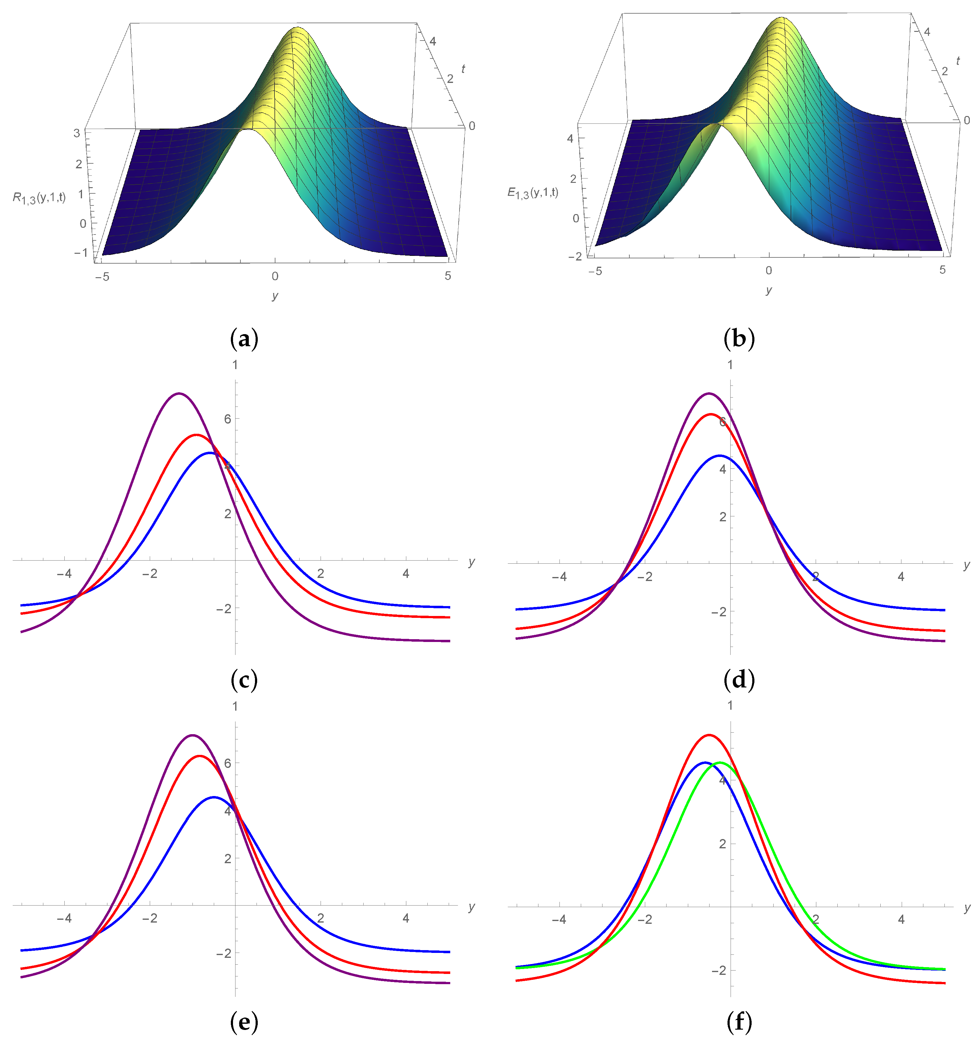
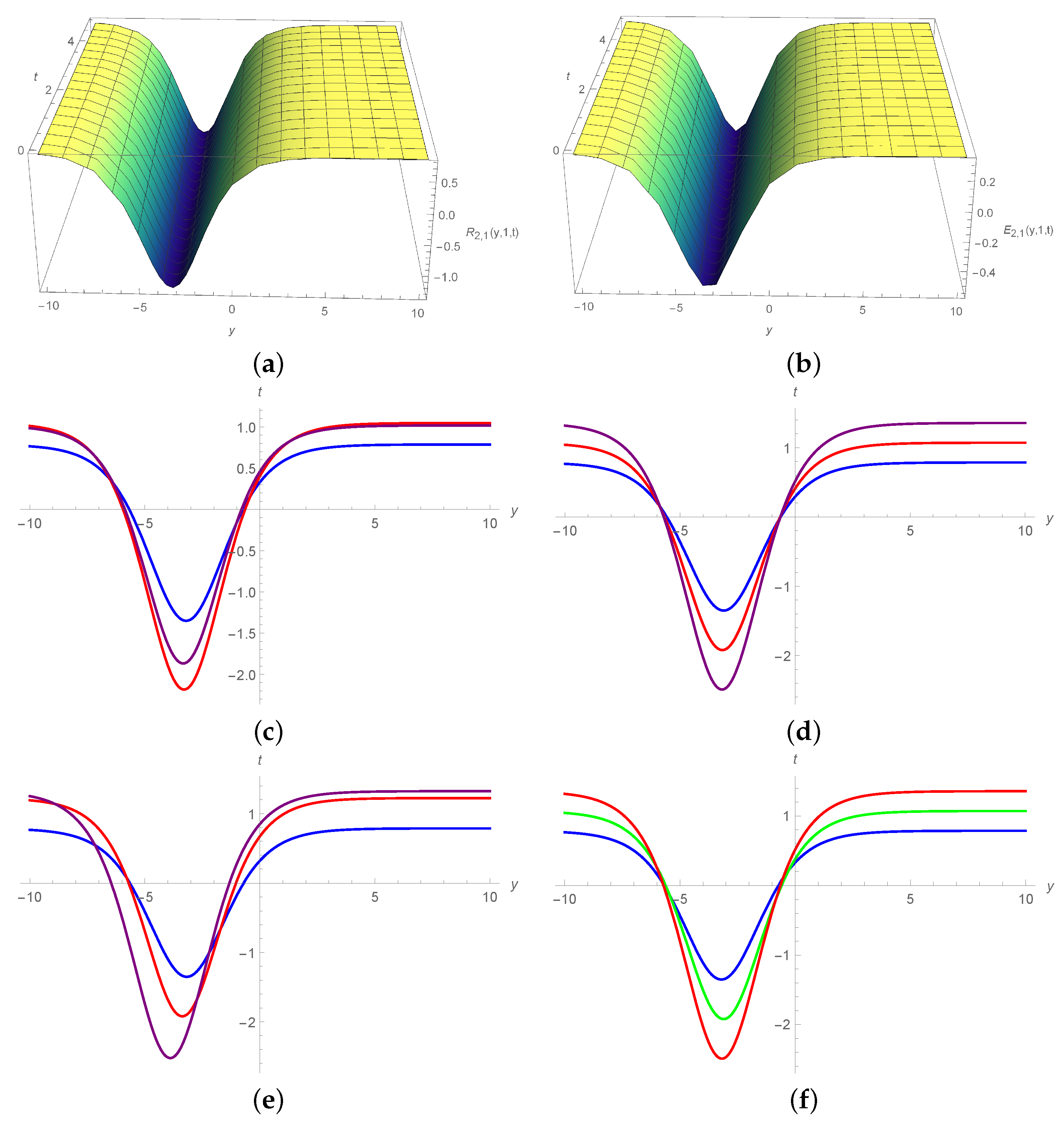
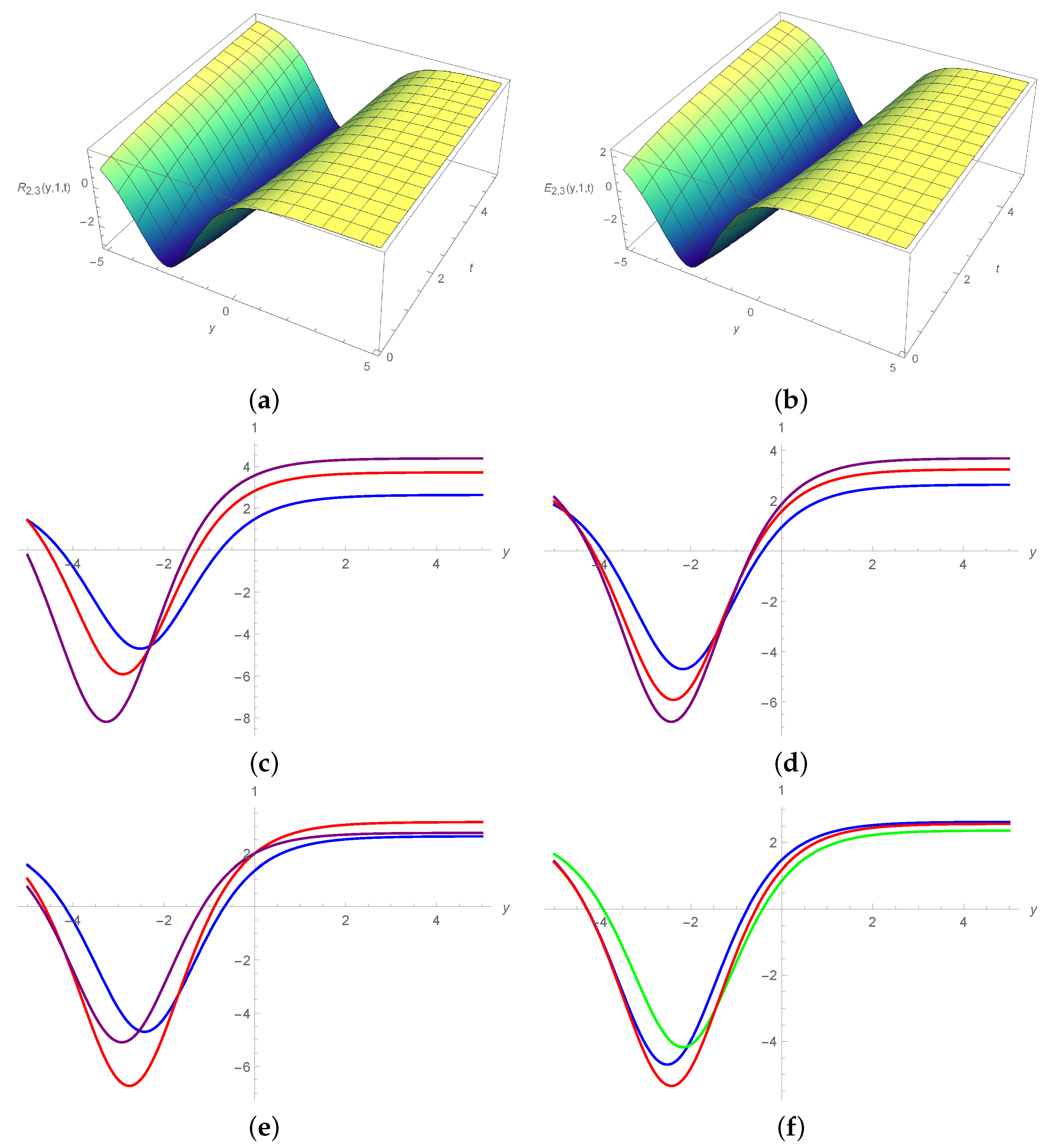
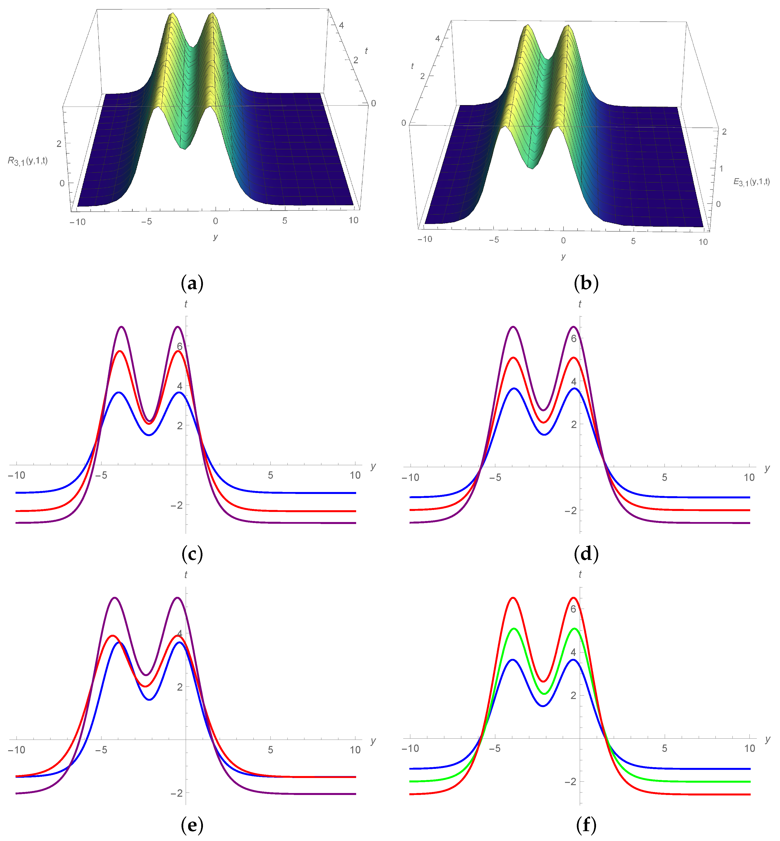
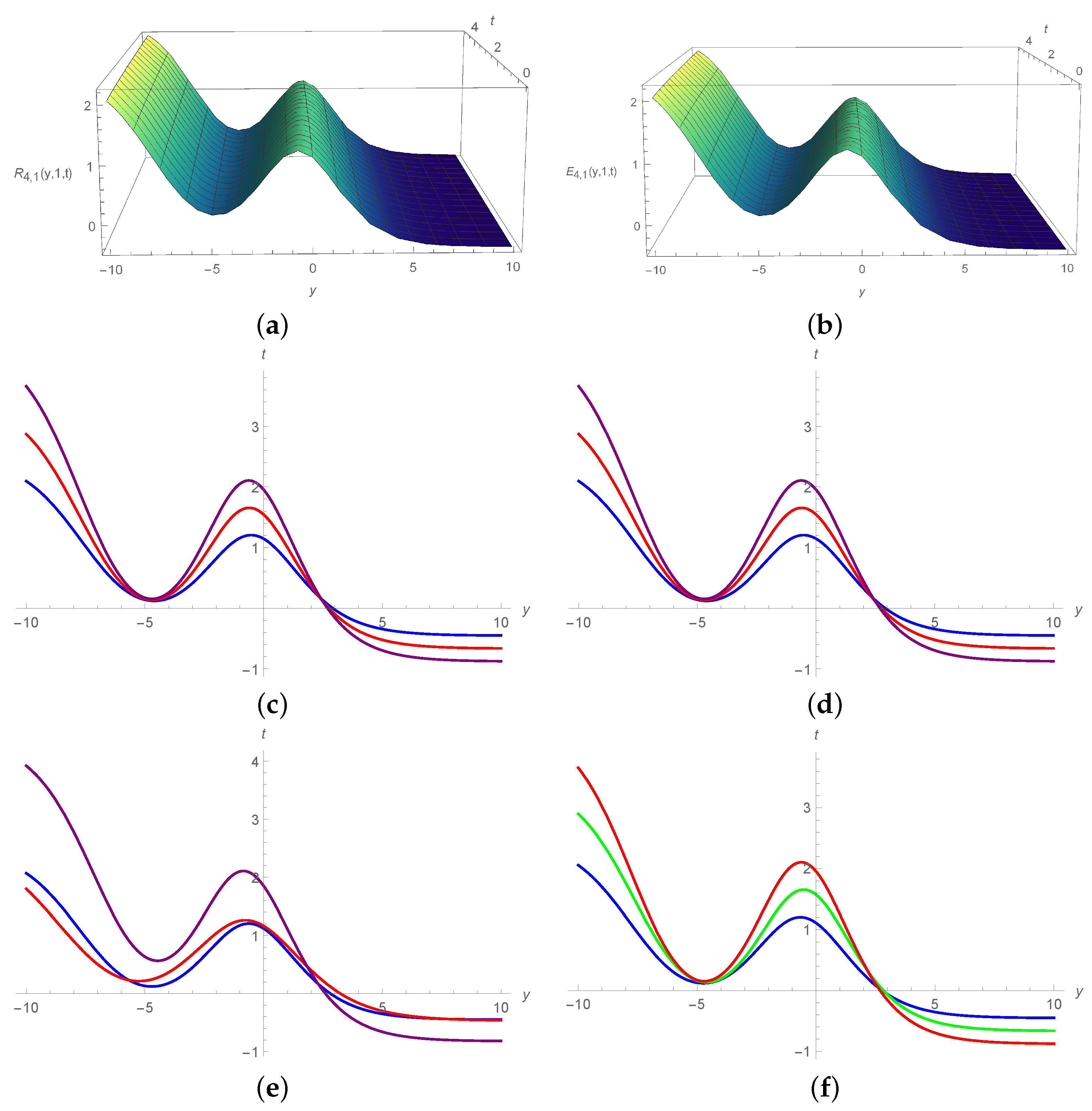
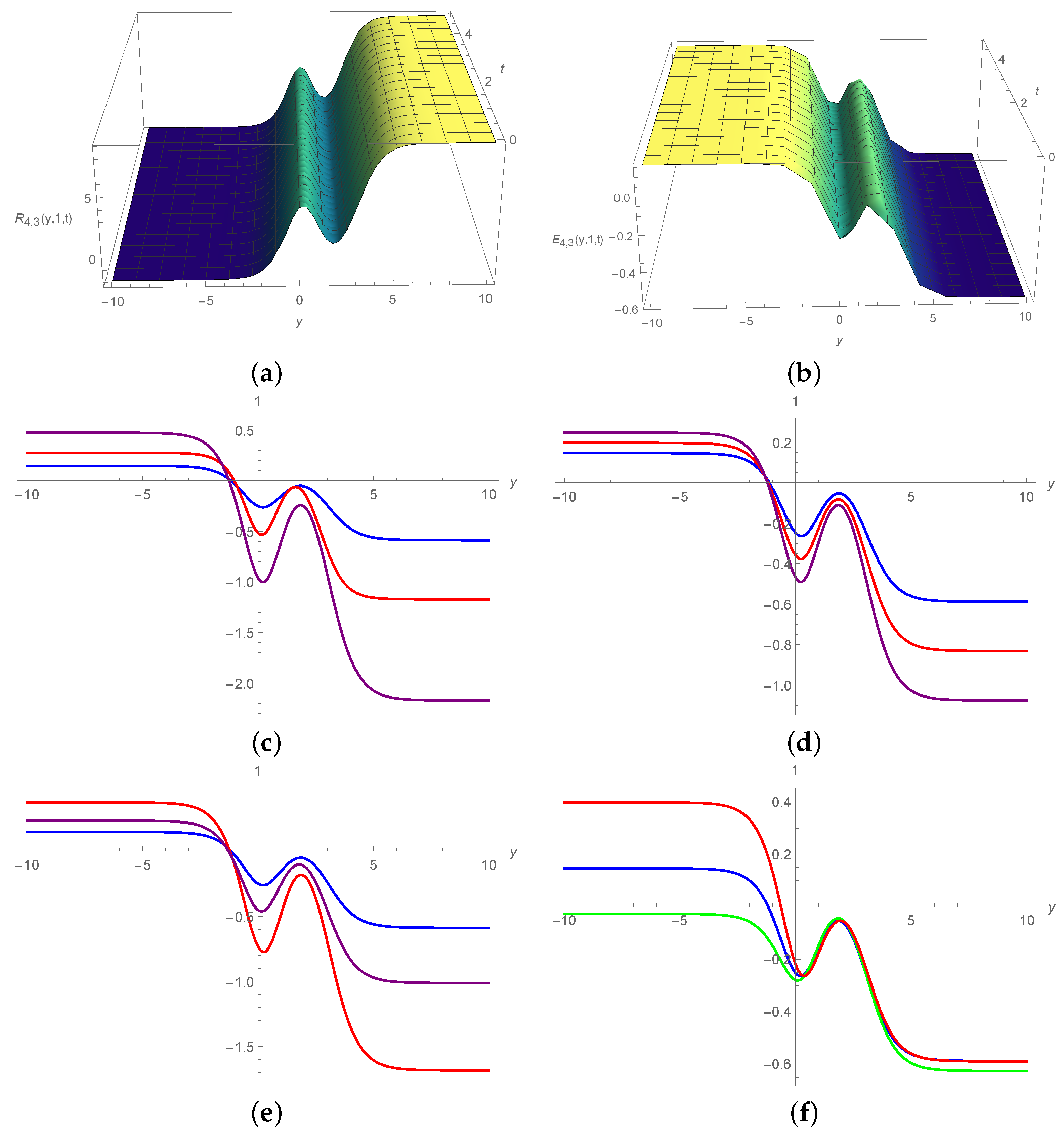
5. Results and Discussion
6. Conclusions
Author Contributions
Funding
Institutional Review Board Statement
Informed Consent Statement
Data Availability Statement
Acknowledgments
Conflicts of Interest
References
- Ablowitz, M.J.; Ramani, A.; Segur, H. Nonlinear evolution equations and ordinary differential equations of Painleve’type. Lett. Nuovo Cim. 1978, 23, 333–338. [Google Scholar] [CrossRef]
- Tikhonov, A.N.; Samarskiy, A.A. Equations of Mathematical Physics; Moscow University Press: Moscow, Russia, 1999. [Google Scholar]
- Renardy, M.; Rogers, R.C. An Introduction to Partial Differential Equations; Springer Science & Business Media: Berlin/Heidelberg, Germany, 2006. [Google Scholar]
- Suret, P.; Tikan, A.; Bonnefoy, F.; Copie, F.; Ducrozet, G.; Gelash, A.; Prabhudesai, G.; Michel, G.; Cazaubiel, A.; Falcon, E.; et al. Nonlinear spectral synthesis of soliton gas in deep-water surface gravity waves. Phys. Rev. Lett. 2020, 125, 264101. [Google Scholar] [CrossRef]
- Barkan, A.; D’angelo, N.; Merlino, R.L. Experiments on ion-acoustic waves in dusty plasmas. Planet. Space Sci. 1996, 44, 239–242. [Google Scholar] [CrossRef]
- Dalir, M.; Bashour, M. Applications of fractional calculus. Appl. Math. Sci. 2010, 4, 1021–1032. [Google Scholar]
- Kilbas, A.A.; Srivastava, H.M.; Trujillo, J.J. Theory and Applications of Fractional Differential Equations; Elsevier: Amsterdam, The Netherlands, 2006. [Google Scholar]
- Sun, H.; Zhang, Y.; Baleanu, D.; Chen, W.; Chen, Y. A new collection of real world applications of fractional calculus in science and engineering. Commun. Nonlinear Sci. Numer. Simul. 2018, 64, 213–231. [Google Scholar] [CrossRef]
- Arnol’d, V.I. Geometrical Methods in the Theory of Ordinary Differential Equations; Springer: Heidelberg/Berlin, Germany, 1983. [Google Scholar]
- Almeida, R. A Caputo fractional derivative of a function with respect to another function. Commun. Nonlinear Sci. Numer. Simul. 2017, 44, 460–481. [Google Scholar] [CrossRef] [Green Version]
- Garg, V.; Singh, K. An improved Grunwald-Letnikov fractional differential mask for image texture enhancement. Int. J. Adv. Comput. Sci. Appl. 2012, 3, 130–135. [Google Scholar] [CrossRef] [Green Version]
- Onder, I.; Cinar, M.; Secer, A.; Bayram, M. Analytical solutions of simplified modified Camassa-Holm equation with conformable and M-truncated derivatives: A comparative study. J. Ocean. Eng. Sci. 2022, in press. [Google Scholar] [CrossRef]
- Atangana, A.; Koca, I. Chaos in a simple nonlinear system with Atangana–Baleanu derivatives with fractional order. Chaos Solitons Fractals 2016, 89, 447–454. [Google Scholar] [CrossRef]
- Atangana, A.; Doungmo Goufo, E.F. Extension of matched asymptotic method to fractional boundary layers problems. Math. Probl. Eng. 2014, 2014, 107535. [Google Scholar] [CrossRef] [Green Version]
- Hussain, A.; Jhangeer, A.; Abbas, N.; Khan, I.; Sherif, E.S.M. Optical solitons of fractional complex Ginzburg–Landau equation with conformable, beta, and M-truncated derivatives: A comparative study. Adv. Differ. Eq. 2020, 2020, 1–19. [Google Scholar] [CrossRef]
- Alharbi, F.M.; Baleanu, D.; Ebaid, A. Physical properties of the projectile motion using the conformable derivative. Chin. J. Phys. 2019, 58, 18–28. [Google Scholar] [CrossRef]
- Majid, S.Z.; Faridi, W.A.; Asjad, M.I.; Abd El-Rahman, M.; Eldin, S.M. Explicit Soliton Structure Formation for the Riemann Wave Equation and a Sensitive Demonstration. Fractal Fract. 2023, 7, 102. [Google Scholar] [CrossRef]
- Barman, H.K.; Seadawy, A.R.; Akbar, M.A.; Baleanu, D. Competent closed form soliton solutions to the Riemann wave equation and the Novikov-Veselov equation. Results Phys. 2020, 17, 103131. [Google Scholar] [CrossRef]
- Triggiani, R. Carleman estimates with no lower-order terms for general Riemann wave equations. Global uniqueness and observability in one shot. Appl. Math. Optim. 2002, 46, 331–375. [Google Scholar]
- Shakeel, M.; Ahmad, B.; Shah, N.A.; Chung, J.D. Solitons Solution of Riemann Wave Equation via Modified Exp Function Method. Symmetry 2022, 14, 2574. [Google Scholar]
- Parkes, E.J.; Duffy, B.R.; Abbott, P.C. The Jacobi elliptic-function method for finding periodic-wave solutions to nonlinear evolution equations. Phys. Lett. A 2002, 295, 280–286. [Google Scholar] [CrossRef]
- Bashar, M.H.; Inc, M.; Islam, S.R.; Mahmoud, K.H.; Akbar, M.A. Soliton solutions and fractional effects to the time-fractional modified equal width equation. Alex. Eng. J. 2022, 61, 12539–12547. [Google Scholar] [CrossRef]
- Podlubny, I. Fractional Differential Equations: An Introduction to Fractional Derivatives, Fractional Differential Equations, to Methods of Their Solution and Some of Their Applications; Academic Press: New York, NY, USA, 1998; p. 198. [Google Scholar]
- Oldham, K.B.; Spanier, J. The Fractional Calculus; Academic Press: New York, NY, USA, 1974. [Google Scholar]
- Singh, J.; Kumar, D.; Al Qurashi, M.; Baleanu, D. A new fractional model for giving up smoking dynamics. Adv. Differ. Eq. 2017, 2017, 88. [Google Scholar] [CrossRef] [Green Version]
- Caputo, M.; Mainardi, F. A new dissipation model based on memory mechanism. Pure Appl. Geophys. 1971, 91, 134–147. [Google Scholar] [CrossRef]
- Caputo, M.; Fabricio, M. A new definition of fractional derivative without singular kernel. Prog. Fract. Differ. Appl. 2019, 1, 73–85. [Google Scholar]
- Atangana, A.; Baleanu, D. New fractional derivatives with nonlocal and non-singular kernel. Theory and application to heat transfer model. Therm. Sci. 2016, 20, 763–769. [Google Scholar] [CrossRef] [Green Version]
- Khalil, R.; Al Horani, M.; Yousef, A.; Sababheh, M. A new definition of fractional derivative. J. Comput. Appl. Math. 2014, 264, 65–70. [Google Scholar] [CrossRef]
- Atangana, A.; Baleanu, D.; Alsaedi, A. New properties of conformable derivative. Open Math. 2015, 13, 1–10. [Google Scholar] [CrossRef]
- Hyder, A.A.; Soliman, A.H. An extended Kudryashov technique for solving stochastic nonlinear models with generalized conformable derivatives. Commun. Nonlinear Sci. Numer. Simul. 2021, 97, 105730. [Google Scholar] [CrossRef]
- Arafat, S.Y.; Islam, S.R.; Rahman, M.M.; Saklayen, M.A. On nonlinear optical solitons of fractional Biswas-Arshed Model with beta derivative. Results Phys. 2023, 48, 106426. [Google Scholar] [CrossRef]
- Atangana, A.; Baleanu, D.; Alsaedi, A. Analysis of time-fractional Hunter–Saxton equation: A model of neumatic liquid crystal. Open Phys. 2016, 14, 145–149. [Google Scholar] [CrossRef]
- Pólya, G. On the mean-value theorem corresponding to a given linear homogeneous differential equation. Trans. Am. Math. Soc. 1922, 24, 312–324. [Google Scholar]
- Kilbas, A.A.; Saigo, M.; Saxena, R.K. Generalized Mittag-Leffler function and generalized fractional calculus operators. Integral Transform. Spec. Funct. 2004, 15, 31–49. [Google Scholar] [CrossRef]
- Serkin, V.N.; Hasegawa, A. Novel soliton solutions of the nonlinear Schrödinger equation model. Phys. Rev. Lett. 2000, 85, 4502. [Google Scholar] [CrossRef]
- Fan, E.; Zhang, J. Applications of the Jacobi elliptic function method to special-type nonlinear equations. Phys. Lett. A 2002, 305, 383–392. [Google Scholar] [CrossRef]
- Dai, C.; Zhang, J. Jacobian elliptic function method for nonlinear differential-difference equations. Chaos Solitons Fractals 2006, 27, 1042–1047. [Google Scholar] [CrossRef]
- Liu, S.; Fu, Z.; Liu, S.; Zhao, Q. Jacobi elliptic function expansion method and periodic wave solutions of nonlinear wave equations. Phys. Lett. A 2006, 289, 69–74. [Google Scholar] [CrossRef]
- Shen, S.; Pan, Z. A note on the Jacobi elliptic function expansion method. Phys. Lett. A 2003, 308, 143–148. [Google Scholar] [CrossRef]
- Liu, G.T.; Fan, T.Y. New applications of developed Jacobi elliptic function expansion methods. Phys. Lett. A 2005, 345, 161–166. [Google Scholar] [CrossRef]
- Islam, S.R.; Wang, H. Some analytical soliton solutions of the nonlinear evolution equations. J. Ocean. Eng. Sci. 2022, in press. [Google Scholar] [CrossRef]
- Wang, M.; Zhou, Y.; Li, Z. Application of a homogeneous balance method to exact solutions of nonlinear equations in mathematical physics. Phys. Lett. A 1996, 216, 67–75. [Google Scholar] [CrossRef]
- Wang, Z.L.; Sun, L.J.; Hua, R.; Zhang, L.H.; Wang, H.F. Lie Symmetry Analysis, Particular Solutions and Conservation Laws of Benjiamin Ono Equation. Symmetry 2022, 14, 9. [Google Scholar] [CrossRef]
- Huo, C.; Li, L. Lie Symmetry Analysis, Particular Solutions and Conservation Laws of a New Extended (3+1)-Dimensional Shallow Water Wave Equation. Symmetry 2022, 14, 1855. [Google Scholar] [CrossRef]
- Akram, G.; Sadaf, M.; Zainab, I. The dynamical study of Biswas–Arshed equation via modified auxiliary equation method. Optik 2022, 255, 168614. [Google Scholar] [CrossRef]
- Akram, G.; Sadaf, M.; Abbas, M.; Zainab, I.; Gillani, S.R. Efficient techniques for traveling wave solutions of time-fractional Zakharov–Kuznetsov equation. Math. Comput. Simul. 2022, 193, 607–622. [Google Scholar] [CrossRef]
- Khater, M.M.; Lu, D.; Attia, R.A. Dispersive long wave of nonlinear fractional Wu-Zhang system via a modified auxiliary equation method. AIP Adv. 2019, 9, 25003. [Google Scholar] [CrossRef] [Green Version]
- Khater, M.M.; Attia, R.A.; Lu, D. Modified auxiliary equation method versus three nonlinear fractional biological models in present explicit wave solutions. Math. Comput. Appl. 2018, 24, 1. [Google Scholar] [CrossRef] [Green Version]
- Wang, X.; Ehsan, H.; Abbas, M.; Akram, G.; Sadaf, M.; Abdeljawad, T. Analytical solitary wave solutions of a time-fractional thin-film ferroelectric material equation involving beta-derivative using modified auxiliary equation method. Results Phys. 2023, 48, 106411. [Google Scholar] [CrossRef]
- Mohammed, W.W.; Cesarano, C.; Al-Askar, F.M. Solutions to the (4+ 1)-Dimensional Time-Fractional Fokas Equation with M-Truncated Derivative. Mathematics 2022, 11, 194. [Google Scholar] [CrossRef]
- Sousa, J.V.D.C.; de Oliveira, E.C. A new truncated M-fractional derivative type unifying some fractional derivative types with classical properties. Int. J. Anal. Appl. 2018, 16, 83–96. [Google Scholar]
- Akram, G.; Arshed, S.; Sadaf, M.; Farooq, K. A study of variation in dynamical behavior of fractional complex Ginzburg-Landau model for different fractional operators. Ain Shams Eng. J. 2023, 14, 102120. [Google Scholar] [CrossRef]
- Shahen, N.H.M.; Bashar, M.H.; Ali, M.S. Dynamical analysis of long-wave phenomena for the nonlinear conformable space-time fractional (2+ 1)-dimensional AKNS equation in water wave mechanics. Heliyon 2020, 6, e05276. [Google Scholar] [CrossRef]


Disclaimer/Publisher’s Note: The statements, opinions and data contained in all publications are solely those of the individual author(s) and contributor(s) and not of MDPI and/or the editor(s). MDPI and/or the editor(s) disclaim responsibility for any injury to people or property resulting from any ideas, methods, instructions or products referred to in the content. |
© 2023 by the authors. Licensee MDPI, Basel, Switzerland. This article is an open access article distributed under the terms and conditions of the Creative Commons Attribution (CC BY) license (https://creativecommons.org/licenses/by/4.0/).
Share and Cite
Ansar, R.; Abbas, M.; Mohammed, P.O.; Al-Sarairah, E.; Gepreel, K.A.; Soliman, M.S. Dynamical Study of Coupled Riemann Wave Equation Involving Conformable, Beta, and M-Truncated Derivatives via Two Efficient Analytical Methods. Symmetry 2023, 15, 1293. https://doi.org/10.3390/sym15071293
Ansar R, Abbas M, Mohammed PO, Al-Sarairah E, Gepreel KA, Soliman MS. Dynamical Study of Coupled Riemann Wave Equation Involving Conformable, Beta, and M-Truncated Derivatives via Two Efficient Analytical Methods. Symmetry. 2023; 15(7):1293. https://doi.org/10.3390/sym15071293
Chicago/Turabian StyleAnsar, Rimsha, Muhammad Abbas, Pshtiwan Othman Mohammed, Eman Al-Sarairah, Khaled A. Gepreel, and Mohamed S. Soliman. 2023. "Dynamical Study of Coupled Riemann Wave Equation Involving Conformable, Beta, and M-Truncated Derivatives via Two Efficient Analytical Methods" Symmetry 15, no. 7: 1293. https://doi.org/10.3390/sym15071293