
Computational Analysis for Fréchet Parameters of Life from Generalized Type-II Progressive Hybrid Censored Data with Applications in Physics and Engineering


Abstract
:1. Introduction
- PHC-T1 if .
- PHC-T2 if .
- Hybrid-T1 if , .
- Hybrid-T2 if , .
- Type-I censoring if , , .
- Type-II censoring if , , .

| 1 | ||||
| 2 | m | 1 | 0 | |
| 3 |
2. Likelihood Inference
3. Bayes Inference
- Step-1:
- Set the starting values and .
- Step-2:
- Set .
- Step-3:
- Create and from and , respectively.
- Step-4:
- Find and .
- Step-5:
- Create samples and using the uniform distribution.
- Step-6:
- If both and are less than and , respectively, then set and , respectively. Otherwise, set and , respectively.
- Step-7:
- Set .
- Step-8:
- Redo steps 3–7 times to get and for .
- Step-9:
- Use and , for , to compute the reliability and hazard rate parameters, respectively, as
4. Interval Inference
4.1. Asymptotic Intervals
4.2. HPD Intervals
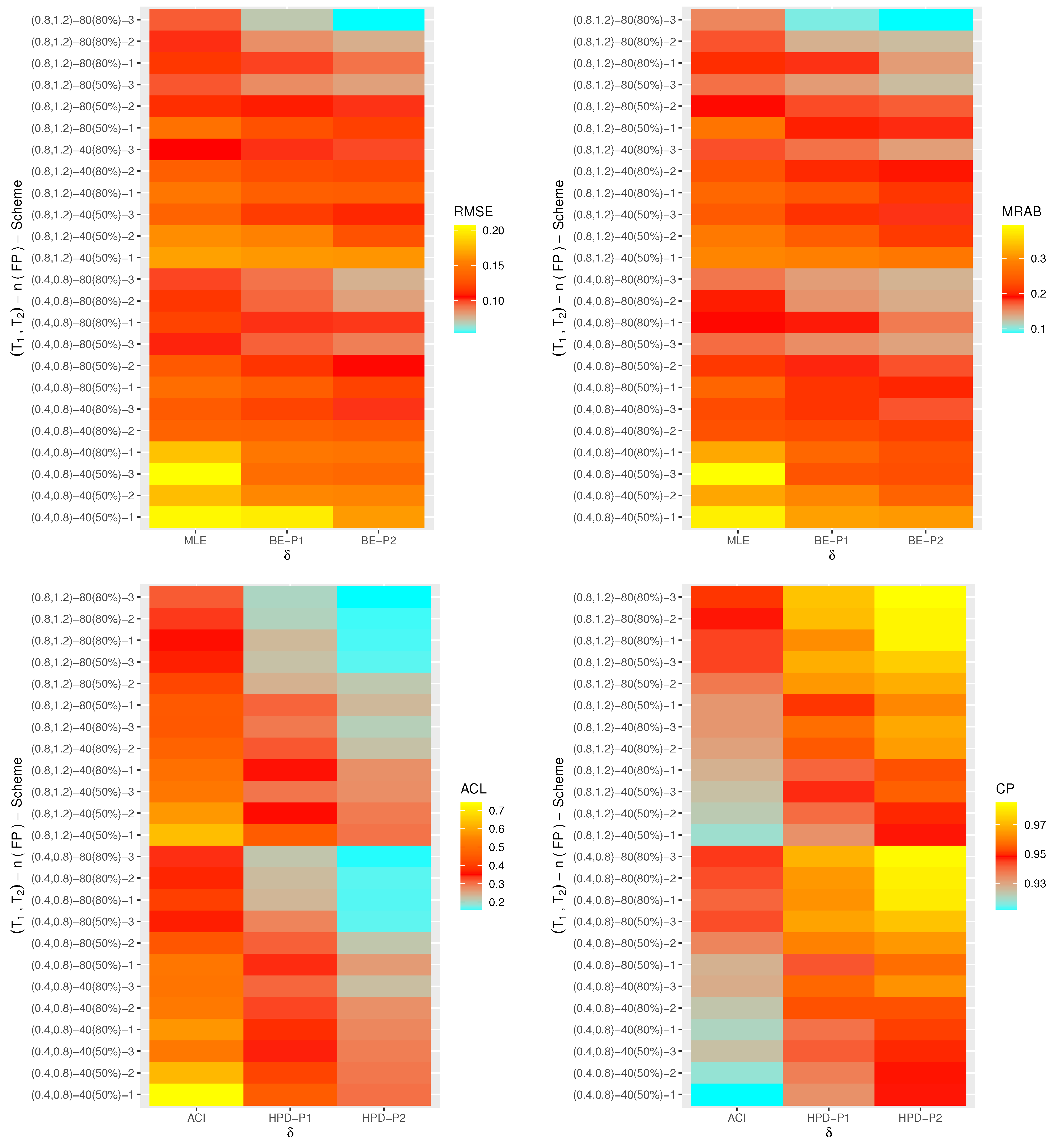
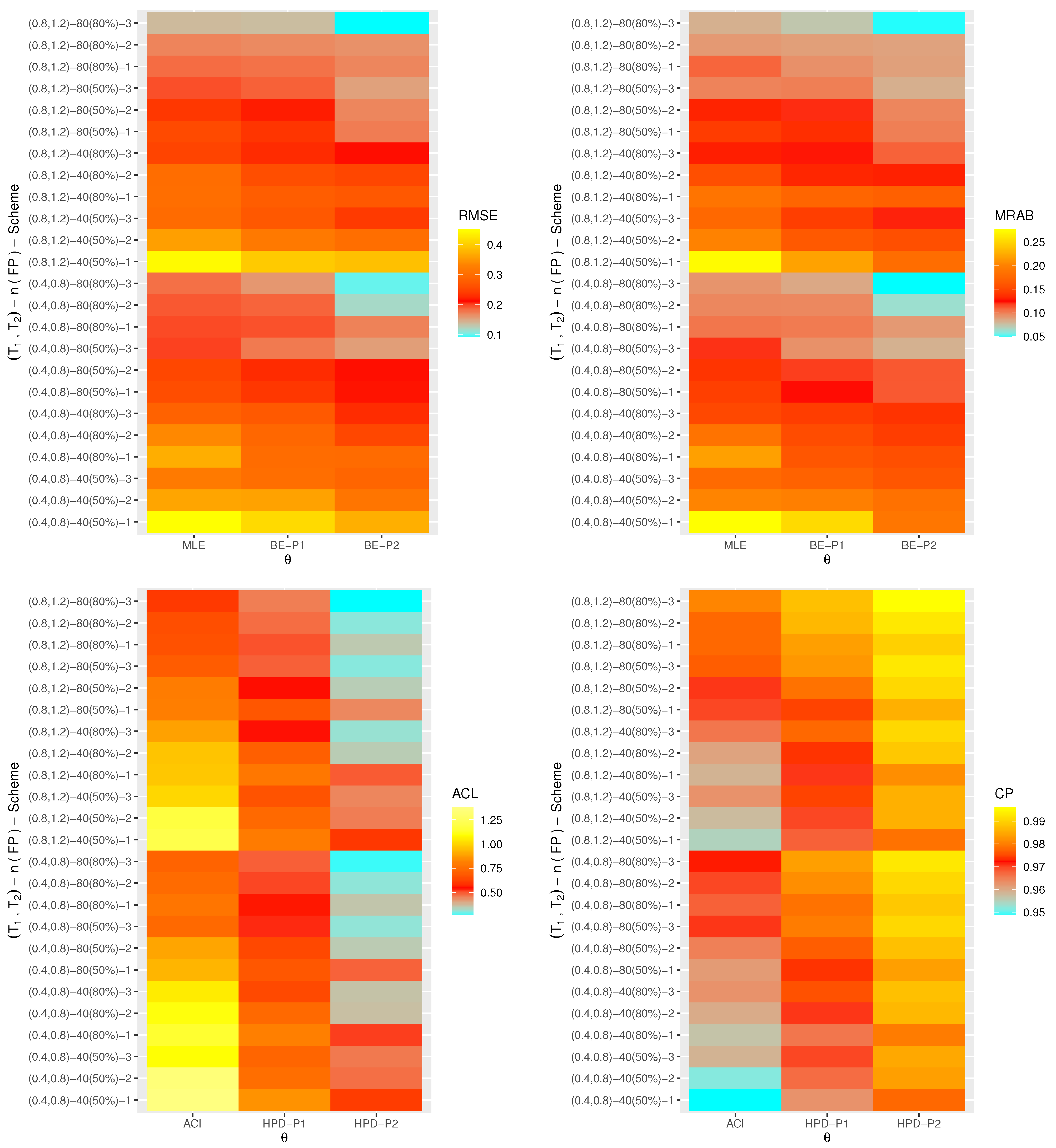
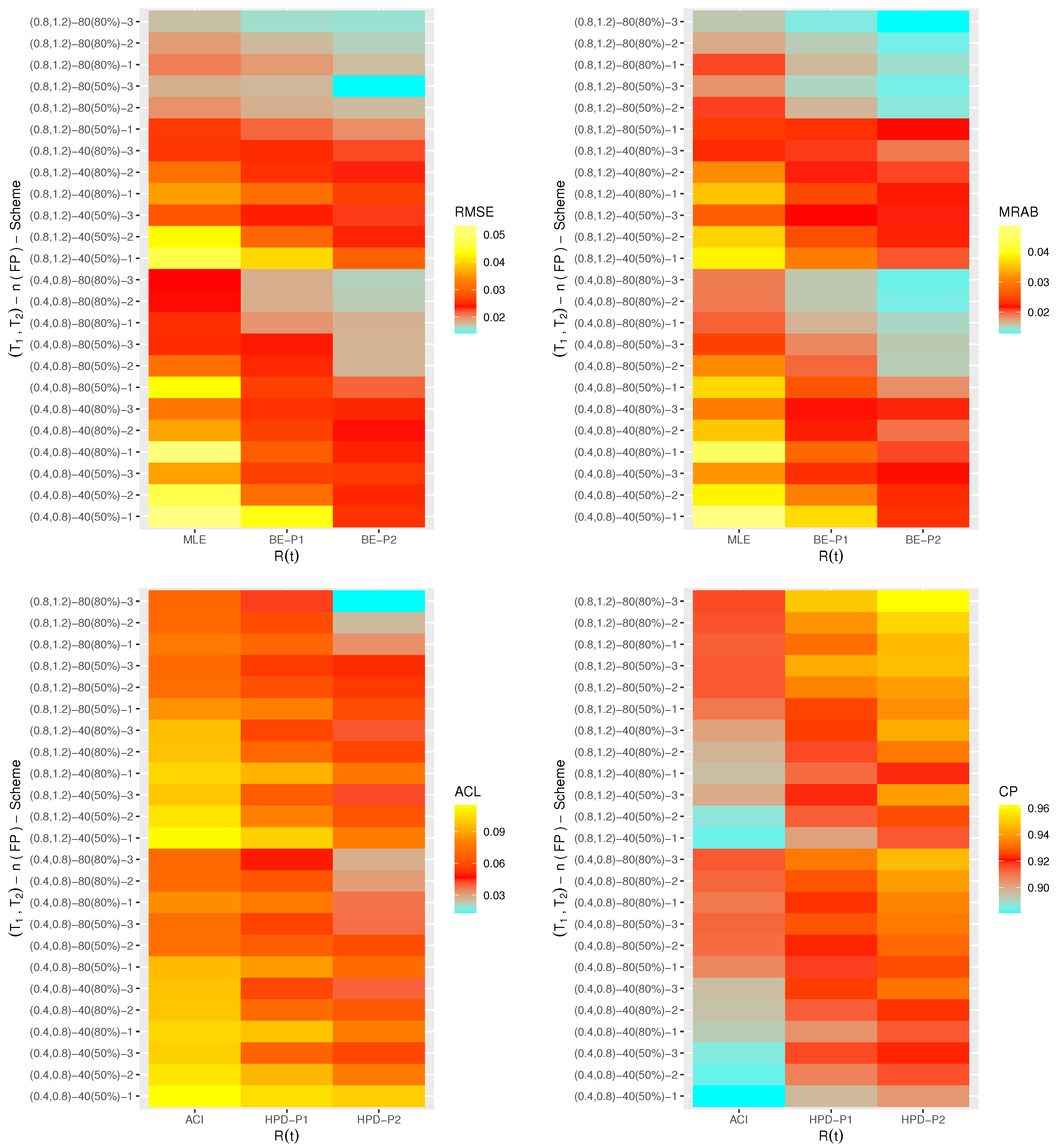
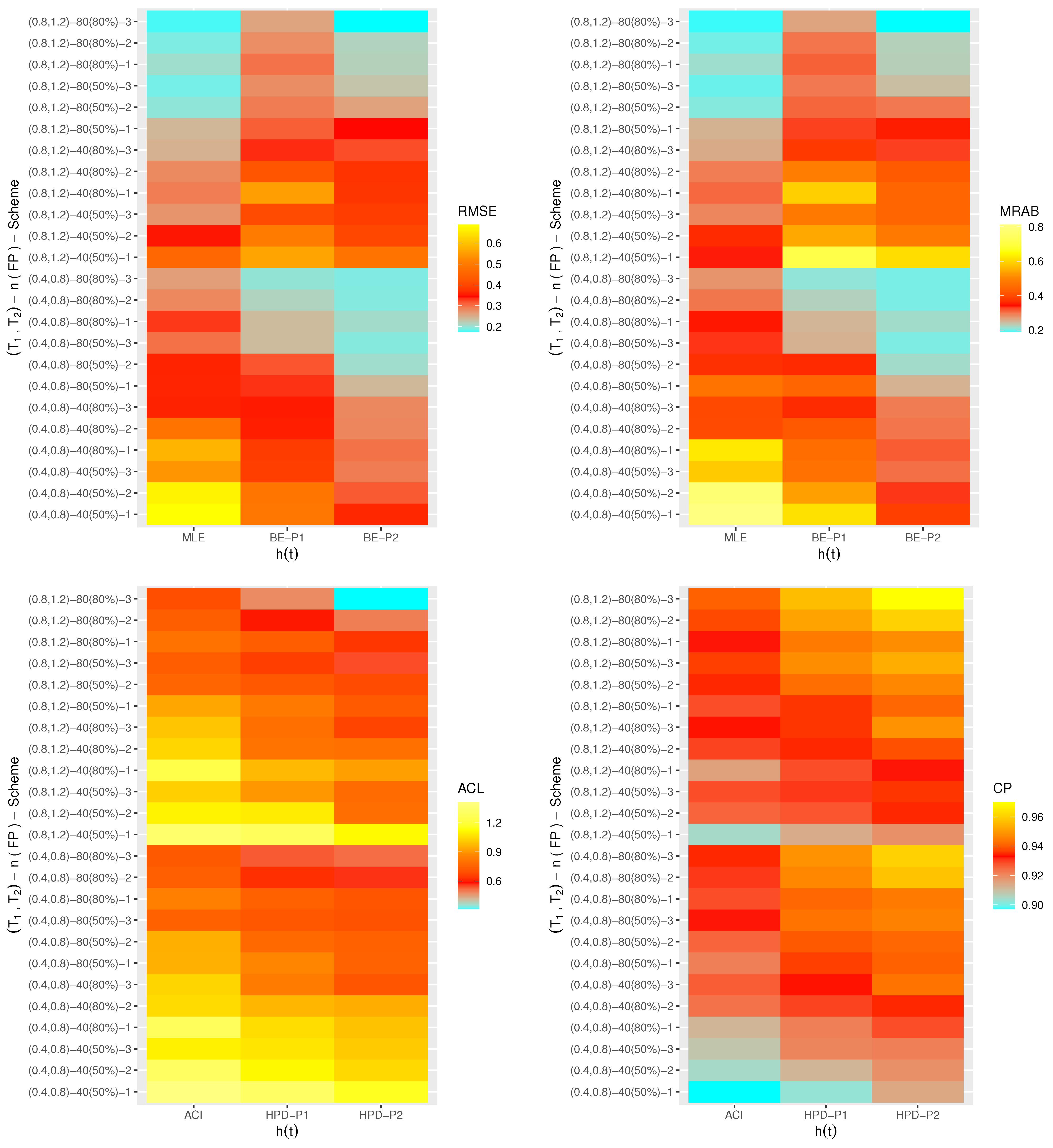
5. Monte Carlo Simulation
- The main general point is that the proposed estimates of , , , or provided good performance.
- As n(or m) increased, all estimates of , , and performed satisfactory. A similar result was obtained when decreased.
- As increased, in most situations, the RMSEs, MRABs, and ACLs of all unknown parameters decreased while their CPs increased.
- The Bayes estimates of , , , or , due to the gamma information, behaved better compared to the other estimates as expected. A similar comment could also be made in the case of HPD credible intervals.
- Since the variance of Prior-II was smaller than the variance of Prior-I, the MCMC calculations under Prior-II provided more accurate estimates than others for all unknown parameters.
- Comparing the proposed schemes 1, 2, and 3, in most cases, it was noted that the proposed estimates of , , , and behaved better using scheme 3 than the others.
- As a result, the Bayes M-H algorithm sampler is recommended to estimate the Fr parameters or its reliability characteristics in the presence of data obtained from generalized Type-II progressive hybrid censoring.
6. Optimal PC-T2 Designs
7. Real-Life Applications
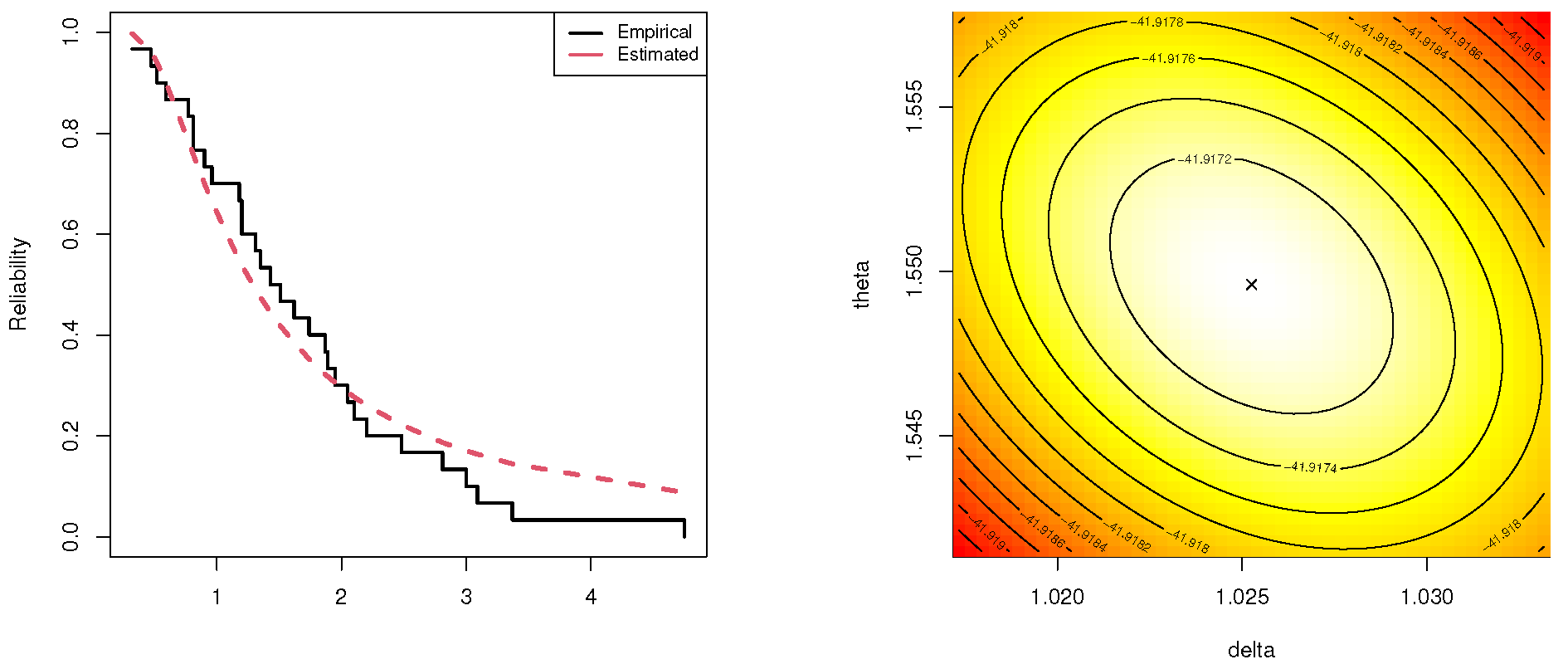
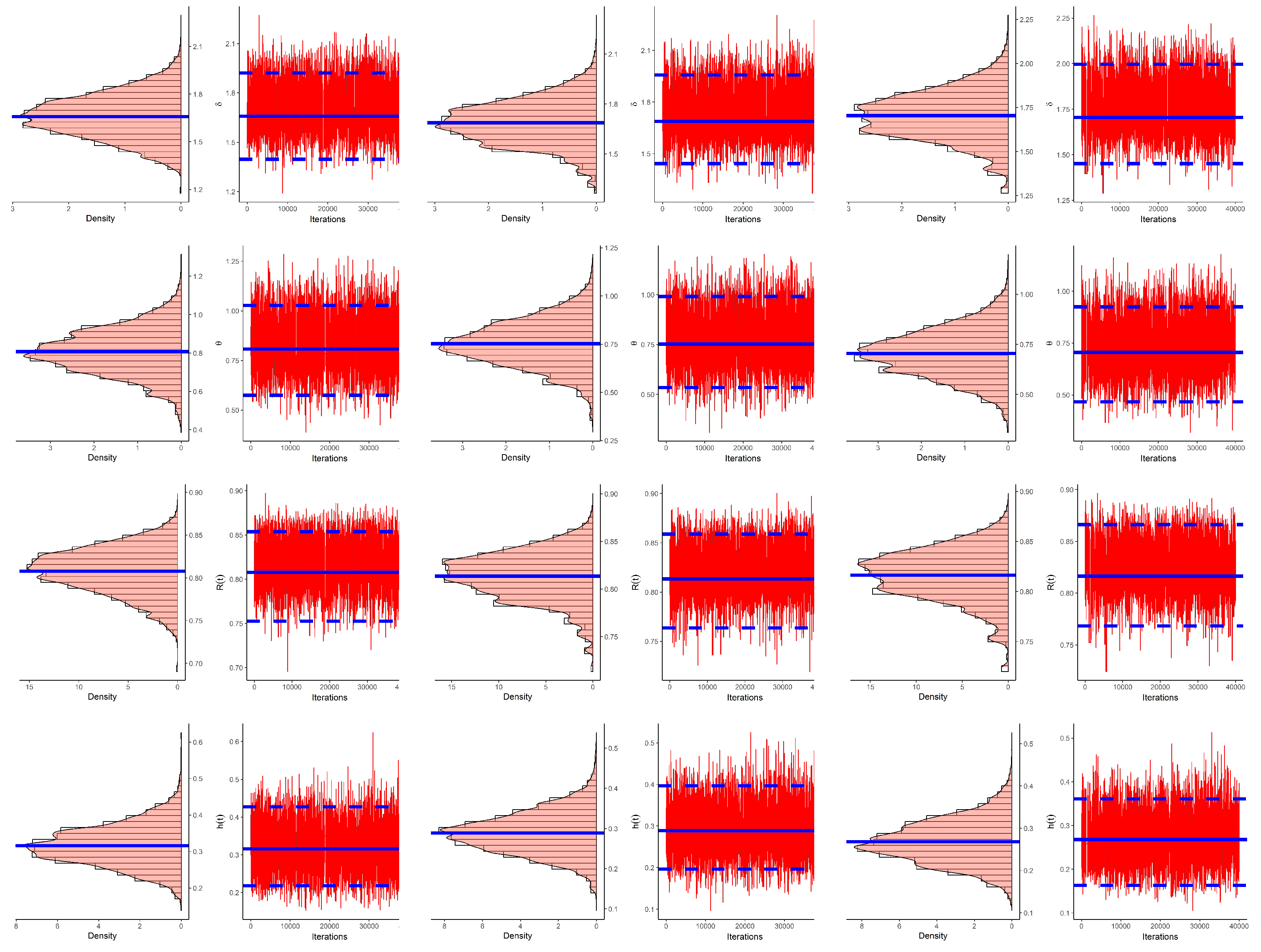
7.1. March Precipitation
- Via criterion , the schemes (in sample 1) and (in samples 2 and 3) were the optimum plans.
- Via criteria , the scheme (in samples 1, 2, and 3) was the optimum plan.
- The ideal PC-T2 plans suggested here confirmed the findings listed in Section 5.
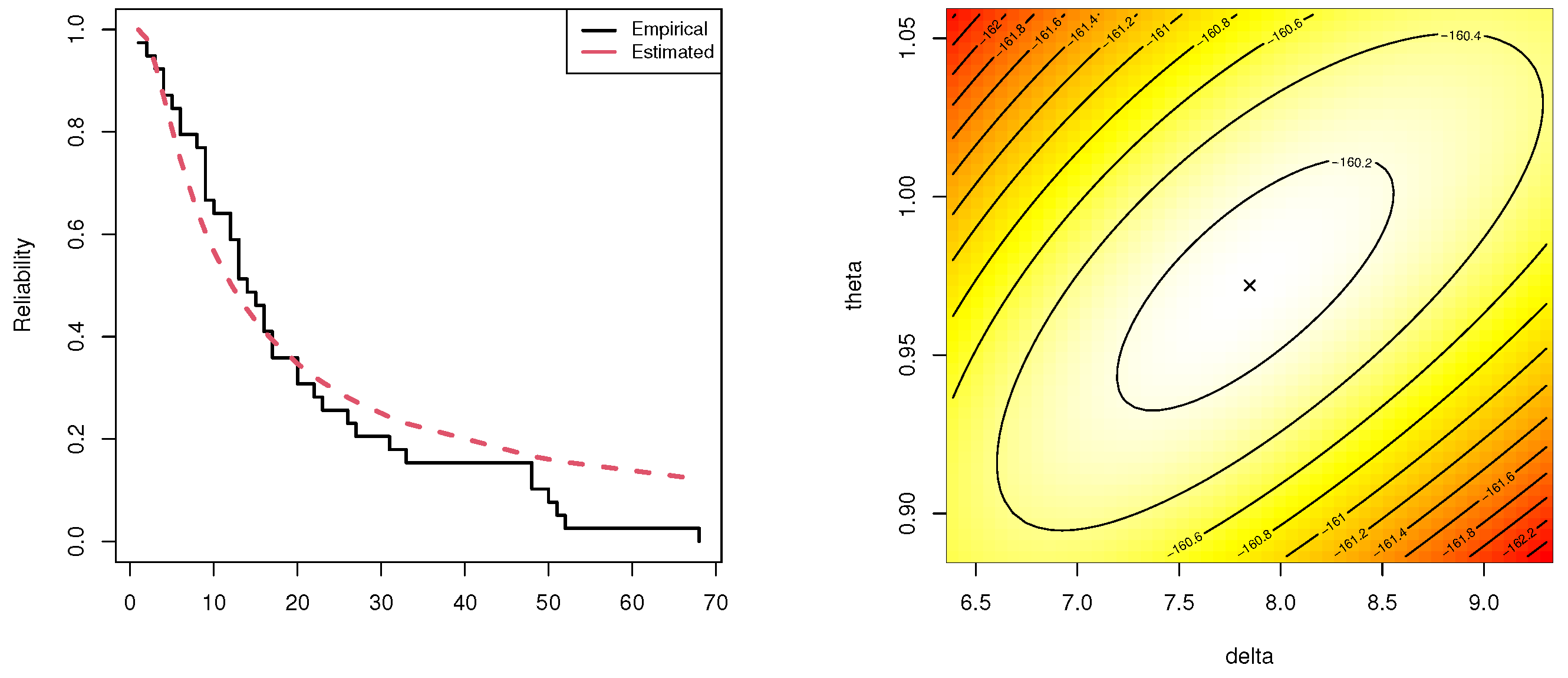
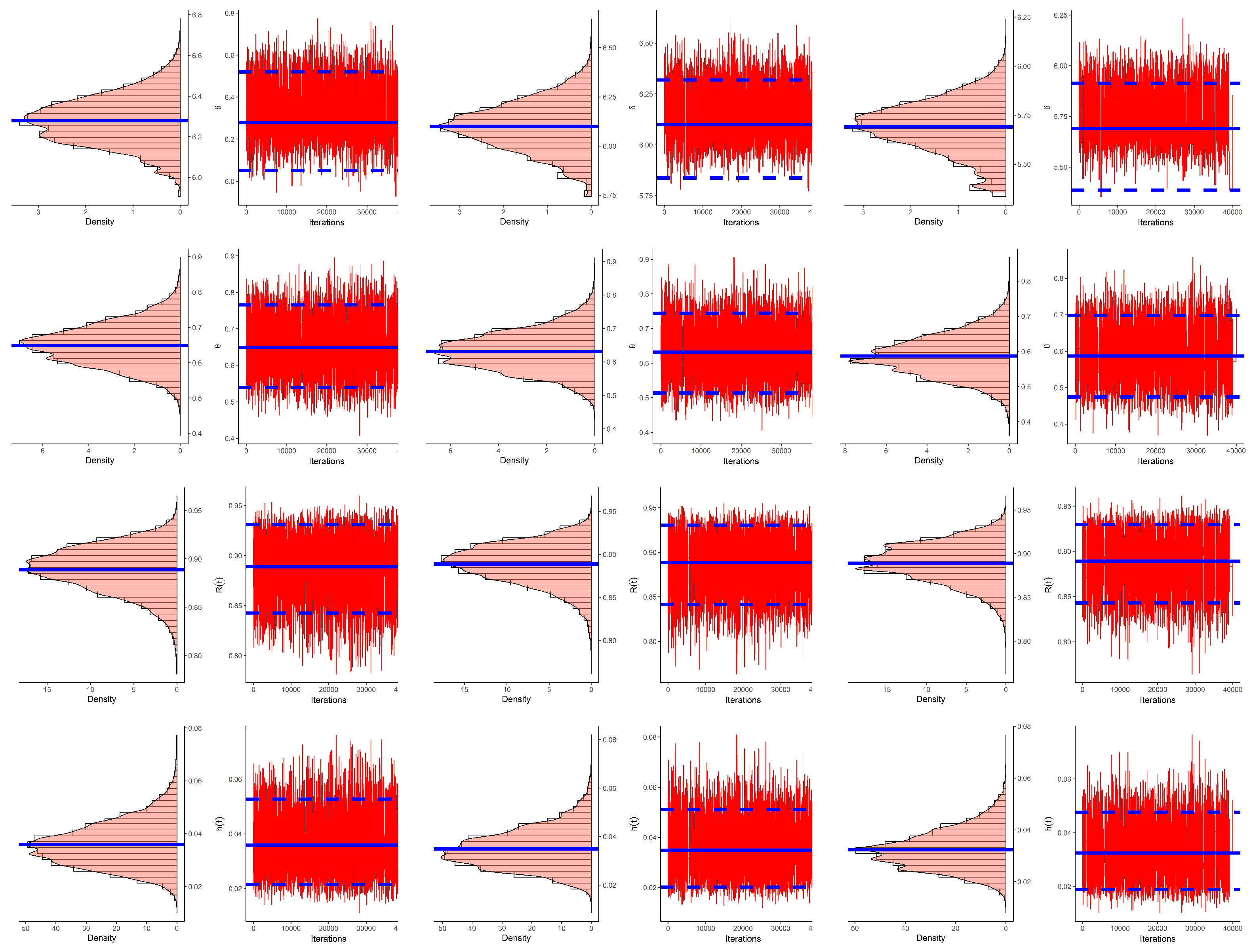
7.2. Vehicle Fatalities
- Via criterion , the schemes (in samples 1 and 2) and (in sample 3) were the optimum plans.
- Via criteria , the scheme (in samples 1, 2, and 3) was the optimum plan.
- Via criterion ; the scheme (in samples 1, 2, and 3) was the optimum plan.
- The ideal PC-T2 plans provided here supported our findings from Section 5 as well.
8. Concluding Remarks
Supplementary Materials
Author Contributions
Funding
Data Availability Statement
Acknowledgments
Conflicts of Interest
References
- Chen, P.; Xu, A.; Ye, Z.S. Generalized fiducial inference for accelerated life tests with Weibull distribution and progressively Type-II censoring. IEEE Trans. Reliab. 2016, 65, 1737–1744. [Google Scholar] [CrossRef]
- Luo, C.; Shen, L.; Xu, A. Modelling and estimation of system reliability under dynamic operating environments and lifetime ordering constraints. Reliab. Eng. Syst. Saf. 2022, 218, 108136. [Google Scholar] [CrossRef]
- Balakrishnan, N.; Cramer, E. The Art of Progressive Censoring; Springer: New York, NY, USA, 2014. [Google Scholar]
- Panahi, H. Interval estimation of Kumaraswamy parameters based on progressively Type II censored sample and record values. Miskolc Math. Notes 2020, 21, 319–334. [Google Scholar] [CrossRef]
- Kundu, D.; Joarder, A. Analysis of Type-II progressively hybrid censored data. Comput. Stat. Data Anal. 2006, 50, 2509–2528. [Google Scholar] [CrossRef]
- Childs, A.; Chandrasekar, B.; Balakrishnan, N. Exact likelihood inference for an exponential parameter under progressive hybrid censoring schemes. In Statistical Models and Methods for Biomedical and Technical Systems; Vonta, F., Nikulin, M., Limnios, N., Huber-Carol, C., Eds.; Springer: Boston, MA, USA, 2008; pp. 319–330. [Google Scholar]
- Panahi, H. Estimation methods for the generalized inverted exponential distribution under Type ii progressively hybrid censoring with application to spreading of micro-drops data. Commun. Math. Stat. 2017, 5, 159–174. [Google Scholar] [CrossRef]
- Ng, H.K.T.; Kundu, D.; Chan, P.S. Statistical analysis of exponential lifetimes under an adaptive Type-II progressive censoring scheme. Nav. Res. Logist. 2009, 56, 687–698. [Google Scholar] [CrossRef] [Green Version]
- Panahi, H.; Moradi, N. Estimation of the inverted exponentiated Rayleigh distribution based on adaptive Type II progressive hybrid censored sample. J. Comput. Appl. Math. 2020, 364, 112345. [Google Scholar] [CrossRef]
- Lee, K.; Sun, H.; Cho, Y. Exact likelihood inference of the exponential parameter under generalized Type II progressive hybrid censoring. J. Korean Stat. Soc. 2016, 45, 123–136. [Google Scholar] [CrossRef]
- Ashour, S.; Elshahhat, A. Bayesian and non-Bayesian estimation for Weibull parameters based on generalized Type-II progressive hybrid censoring scheme. Pak. J. Stat. Oper. Res. 2016, 12, 213–226. [Google Scholar]
- Ateya, S.; Mohammed, H. Prediction under Burr-XII distribution based on generalized Type-II progressive hybrid censoring scheme. J. Egypt. Math. Soc. 2018, 26, 491–508. [Google Scholar]
- Seo, J.I. Objective Bayesian analysis for the Weibull distribution with partial information under the generalized Type-II progressive hybrid censoring scheme. Commun.-Stat.-Simul. Comput. 2020, 51, 5157–5173. [Google Scholar] [CrossRef]
- Cho, S.; Lee, K. Exact Likelihood Inference for a Competing Risks Model with Generalized Type II Progressive Hybrid Censored Exponential Data. Symmetry 2021, 13, 887. [Google Scholar] [CrossRef]
- Nagy, M.; Bakr, M.E.; Alrasheedi, A.F. Analysis with applications of the generalized Type-II progressive hybrid censoring sample from Burr Type-XII model. Math. Probl. Eng. 2022, 2022, 1241303. [Google Scholar] [CrossRef]
- Wang, L.; Zhou, Y.; Lio, Y.; Tripathi, Y.M. Inference for Kumaraswamy Distribution under Generalized Progressive Hybrid Censoring. Symmetry 2022, 14, 403. [Google Scholar] [CrossRef]
- Fréchet, M. Sur la loi de probabilité de lécart maximum. Ann. Soc. Pol. Math. 1927, 6, 93–116. [Google Scholar]
- Kotz, S.; Nadarajah, S. Extreme Value Distributions: Theory and Applications; Imperial College Press: London, UK, 2000. [Google Scholar]
- Henningsen, A.; Toomet, O. maxLik: A package for maximum likelihood estimation in R. Comput. Stat. 2011, 26, 443–458. [Google Scholar] [CrossRef]
- Plummer, M.; Best, N.; Cowles, K.; Vines, K. CODA: Convergence diagnosis and output analysis for MCMC. R News 2006, 6, 7–11. [Google Scholar]
- Gelman, A.; Carlin, J.B.; Stern, H.S.; Rubin, D.B. Bayesian Data Analysis, 2nd ed.; Chapman and Hall/CRC: Boca Raton, FL, USA, 2004. [Google Scholar]
- Lynch, S.M. Introduction to Applied Bayesian Statistics and Estimation for Social Scientists; Springer: New York, NY, USA, 2007. [Google Scholar]
- Lawless, J.F. Statistical Models and Methods for Lifetime Data, 2nd ed.; John Wiley and Sons: Hoboken, NJ, USA, 2003. [Google Scholar]
- Greene, W.H. Econometric Analysis, 4th ed.; Prentice-Hall: New York, NY, USA, 2000. [Google Scholar]
- Chen, M.H.; Shao, Q.M. Monte Carlo estimation of Bayesian credible and HPD intervals. J. Comput. Graph. Stat. 1999, 8, 69–92. [Google Scholar]
- Balakrishnan, N.L.; Aggarwala, R. Progressive Censoring Theory, Methods and Applications; Springer: Boston, MA, USA, 2000. [Google Scholar]
- Ng, H.K.T.; Chan, P.S.; Balakrishnan, N. Optimal progressive censoring plans for the Weibull distribution. Technometrics 2004, 46, 470–481. [Google Scholar] [CrossRef]
- Sen, T.; Tripathi, Y.M.; Bhattacharya, R. Statistical inference and optimum life testing plans under Type-II hybrid censoring scheme. Ann. Data Sci. 2018, 5, 679–708. [Google Scholar] [CrossRef]
- Elshahhat, A.; Abu El Azm, W.S. Statistical reliability analysis of electronic devices using generalized progressively hybrid censoring plan. Qual. Reliab. Eng. Int. 2022, 38, 1112–1130. [Google Scholar] [CrossRef]
- Elshahhat, A.; Mohammed, H.S.; Abo-Kasem, O.E. Reliability Inferences of the Inverted NH Parameters via Generalized Type-II Progressive Hybrid Censoring with Applications. Symmetry 2022, 14, 2379. [Google Scholar] [CrossRef]
- Hinkley, D. On quick choice of power transformation. J. R. Stat. Soc. 1977, 26, 67–69. [Google Scholar] [CrossRef]
- Elshahhat, A.; Bhattacharya, R.; Mohammed, H.S. Survival Analysis of Type-II Lehmann Fréchet Parameters via Progressive Type-II Censoring with Applications. Axioms 2022, 11, 700. [Google Scholar] [CrossRef]
- Mann, S.P. Introductoty Statistics; John Wiley and Sons Inc.: New York, NY, USA, 2016. [Google Scholar]


| Criterion | Target |
|---|---|
| Maximize trace | |
| Minimize trace | |
| Minimize det | |
| Minimize |
| 0.77 | 1.74 | 0.81 | 1.20 | 1.95 | 1.20 | 0.47 | 1.43 | 3.37 | 2.20 |
| 3.00 | 3.09 | 1.51 | 2.10 | 0.52 | 1.62 | 1.31 | 0.32 | 0.59 | 0.81 |
| 2.81 | 1.87 | 1.18 | 1.35 | 4.75 | 2.48 | 0.96 | 1.89 | 0.90 | 2.05 |
| Scheme | Sample | Generated Data | ||||
|---|---|---|---|---|---|---|
| 1 | 3.40(11) | 5.00(11) | 0.32, 0.59, 0.81, 1.18, 1.31, 1.51, 1.87, 2.05, 2.48, 3.09, 3.37 | 1 | 3.40 | |
| 2 | 2.00(7) | 3.25(10) | 0.32, 0.59, 0.81, 1.18, 1.31, 1.51, 1.87, 2.05, 2.48, 3.09 | 0 | 3.09 | |
| 3 | 2.00(7) | 2.50(9) | 0.32, 0.59, 0.81, 1.18, 1.31, 1.51, 1.87, 2.05, 2.48 | 3 | 2.50 | |
| 1 | 2.95(11) | 3.05(11) | 0.32, 0.81, 1.31, 1.35, 1.43, 1.51, 1.62, 1.74, 1.87, 2.48, 2.81 | 4 | 2.95 | |
| 2 | 2.25(9) | 2.50(10) | 0.32, 0.81, 1.31, 1.35, 1.43, 1.51, 1.62, 1.74, 1.87, 2.48 | 0 | 2.48 | |
| 3 | 1.50(5) | 2.00(9) | 0.32, 0.81, 1.31, 1.35, 1.43, 1.51, 1.62, 1.74, 1.87 | 6 | 2.00 | |
| 1 | 3.50(11) | 4.80(11) | 0.32, 0.90, 1.43, 2.05, 2.10, 2.20, 2.48, 2.81, 3.00, 3.09, 3.37 | 1 | 3.50 | |
| 2 | 2.75(7) | 3.25(10) | 0.32, 0.90, 1.43, 2.05, 2.10, 2.20, 2.48, 2.81, 3.00, 3.09 | 0 | 3.09 | |
| 3 | 2.25(6) | 3.05(9) | 0.32, 0.90, 1.43, 2.05, 2.10, 2.20, 2.48, 2.81, 3.00 | 3 | 3.05 | |
| 1 | 2.60(11) | 4.80(11) | 0.32, 0.59, 0.77, 0.81, 0.81, 0.90, 0.96, 1.18, 1.62, 2.20, 2.48 | 5 | 2.60 | |
| 2 | 1.10(7) | 2.50(10) | 0.32, 0.59, 0.77, 0.81, 0.81, 0.90, 0.96, 1.18, 1.62, 2.20 | 0 | 2.20 | |
| 3 | 1.50(8) | 2.10(9) | 0.32, 0.59, 0.77, 0.81, 0.81, 0.90, 0.96, 1.18, 1.62 | 7 | 2.10 |
| Scheme | Sample | Par. | MLE | MCMC | ACI | HPD | ||||||
|---|---|---|---|---|---|---|---|---|---|---|---|---|
| Est. | SE | Est. | SE | Lower | Upper | Width | Lower | Upper | Width | |||
| 1 | 1.8514 | 0.3703 | 1.6588 | 0.2364 | 1.1256 | 2.5772 | 1.4517 | 1.3969 | 1.9224 | 0.5255 | ||
| 0.9547 | 0.1974 | 0.8078 | 0.1878 | 0.5677 | 1.3417 | 0.7739 | 0.5750 | 1.0277 | 0.4527 | |||
| 0.8430 | 0.0581 | 0.8079 | 0.0439 | 0.7290 | 0.9570 | 0.2279 | 0.7526 | 0.8538 | 0.1011 | |||
| 0.3292 | 0.1084 | 0.3162 | 0.0557 | 0.1168 | 0.5416 | 0.4248 | 0.2183 | 0.4275 | 0.2093 | |||
| 2 | 1.8803 | 0.3765 | 1.6879 | 0.2337 | 1.1424 | 2.6182 | 1.4758 | 1.4424 | 1.9576 | 0.5152 | ||
| 0.9039 | 0.1991 | 0.7523 | 0.1922 | 0.5136 | 1.2941 | 0.7804 | 0.5353 | 0.9912 | 0.4559 | |||
| 0.8475 | 0.0574 | 0.8135 | 0.0421 | 0.7349 | 0.9600 | 0.2251 | 0.7637 | 0.8588 | 0.0952 | |||
| 0.3059 | 0.1046 | 0.2889 | 0.0545 | 0.1010 | 0.5108 | 0.4098 | 0.1962 | 0.3969 | 0.2007 | |||
| 3 | 1.9040 | 0.3823 | 1.7049 | 0.2416 | 1.1547 | 2.6534 | 1.4988 | 1.4514 | 1.9965 | 0.5451 | ||
| 0.8633 | 0.2033 | 0.7049 | 0.1974 | 0.4648 | 1.2618 | 0.7970 | 0.4664 | 0.9247 | 0.4583 | |||
| 0.8510 | 0.0570 | 0.8165 | 0.0428 | 0.7394 | 0.9627 | 0.2233 | 0.7685 | 0.8662 | 0.0977 | |||
| 0.2877 | 0.1028 | 0.2679 | 0.0545 | 0.0862 | 0.4892 | 0.4030 | 0.1634 | 0.3608 | 0.1974 | |||
| 1 | 2.3307 | 0.4210 | 2.1201 | 0.2523 | 1.5056 | 3.1559 | 1.6503 | 1.8228 | 2.3704 | 0.5476 | ||
| 0.8229 | 0.1722 | 0.6788 | 0.1806 | 0.4853 | 1.1605 | 0.6752 | 0.4675 | 0.8874 | 0.4199 | |||
| 0.9028 | 0.0409 | 0.8788 | 0.0294 | 0.8226 | 0.9830 | 0.1604 | 0.8466 | 0.9129 | 0.0662 | |||
| 0.2066 | 0.0680 | 0.1969 | 0.0374 | 0.0733 | 0.3398 | 0.2666 | 0.1295 | 0.2686 | 0.1391 | |||
| 2 | 1.8799 | 0.3918 | 1.6843 | 0.2392 | 1.1120 | 2.6479 | 1.5359 | 1.4255 | 1.9528 | 0.5273 | ||
| 1.0014 | 0.2118 | 0.8466 | 0.1956 | 0.5863 | 1.4164 | 0.8301 | 0.6217 | 1.0810 | 0.4594 | |||
| 0.8474 | 0.0598 | 0.8127 | 0.0432 | 0.7302 | 0.9646 | 0.2344 | 0.7596 | 0.8581 | 0.0985 | |||
| 0.3390 | 0.1155 | 0.3261 | 0.0565 | 0.1126 | 0.5654 | 0.4528 | 0.2244 | 0.4378 | 0.2134 | |||
| 3 | 1.8845 | 0.3952 | 1.6894 | 0.2366 | 1.1099 | 2.6591 | 1.5493 | 1.4467 | 1.9610 | 0.5144 | ||
| 0.9891 | 0.2206 | 0.8256 | 0.2046 | 0.5568 | 1.4214 | 0.8647 | 0.6076 | 1.0796 | 0.4720 | |||
| 0.8481 | 0.0600 | 0.8137 | 0.0425 | 0.7304 | 0.9658 | 0.2353 | 0.7646 | 0.8593 | 0.0946 | |||
| 0.3339 | 0.1184 | 0.3168 | 0.0570 | 0.1018 | 0.5660 | 0.4642 | 0.2180 | 0.4256 | 0.2075 | |||
| 1 | 2.3735 | 0.4667 | 2.1580 | 0.2556 | 1.4589 | 3.2882 | 1.8294 | 1.8927 | 2.4194 | 0.5267 | ||
| 0.8882 | 0.1730 | 0.7458 | 0.1808 | 0.5490 | 1.2273 | 0.6783 | 0.5500 | 0.9770 | 0.4269 | |||
| 0.9069 | 0.0435 | 0.8834 | 0.0284 | 0.8216 | 0.9921 | 0.1704 | 0.8529 | 0.9141 | 0.0611 | |||
| 0.2165 | 0.0766 | 0.2109 | 0.0366 | 0.0664 | 0.3667 | 0.3002 | 0.1397 | 0.2787 | 0.1389 | |||
| 2 | 2.0295 | 0.4390 | 1.8276 | 0.2421 | 1.1691 | 2.8898 | 1.7207 | 1.5706 | 2.0924 | 0.5218 | ||
| 1.0130 | 0.2028 | 0.8574 | 0.1962 | 0.6155 | 1.4105 | 0.7950 | 0.6199 | 1.0857 | 0.4658 | |||
| 0.8686 | 0.0577 | 0.8378 | 0.0376 | 0.7555 | 0.9816 | 0.2261 | 0.7953 | 0.8787 | 0.0834 | |||
| 0.3110 | 0.1121 | 0.3012 | 0.0508 | 0.0914 | 0.5307 | 0.4393 | 0.2087 | 0.4009 | 0.1921 | |||
| 3 | 2.0708 | 0.4490 | 1.8624 | 0.2513 | 1.1908 | 2.9508 | 1.7600 | 1.5918 | 2.1203 | 0.5286 | ||
| 0.9542 | 0.2040 | 0.7971 | 0.1973 | 0.5545 | 1.3540 | 0.7996 | 0.5466 | 1.0094 | 0.4627 | |||
| 0.8739 | 0.0566 | 0.8432 | 0.0378 | 0.7630 | 0.9849 | 0.2219 | 0.7990 | 0.8817 | 0.0827 | |||
| 0.2851 | 0.1065 | 0.2737 | 0.0485 | 0.0764 | 0.4938 | 0.4173 | 0.1826 | 0.3615 | 0.1788 | |||
| 1 | 1.7138 | 0.3237 | 1.5320 | 0.2232 | 1.0794 | 2.3482 | 1.2688 | 1.2781 | 1.7873 | 0.5092 | ||
| 0.8887 | 0.2006 | 0.7435 | 0.1850 | 0.4955 | 1.2820 | 0.7865 | 0.5247 | 0.9780 | 0.4532 | |||
| 0.8198 | 0.0583 | 0.7821 | 0.0471 | 0.7055 | 0.9341 | 0.2286 | 0.7277 | 0.8376 | 0.1099 | |||
| 0.3347 | 0.1087 | 0.3149 | 0.0590 | 0.1216 | 0.5478 | 0.4262 | 0.2034 | 0.4170 | 0.2136 | |||
| 2 | 1.6400 | 0.3231 | 1.4614 | 0.2202 | 1.0067 | 2.2733 | 1.2666 | 1.2305 | 1.7284 | 0.4979 | ||
| 0.9122 | 0.2171 | 0.7602 | 0.1941 | 0.4867 | 1.3377 | 0.8510 | 0.5090 | 0.9807 | 0.4717 | |||
| 0.8060 | 0.0627 | 0.7662 | 0.0500 | 0.6832 | 0.9289 | 0.2457 | 0.7115 | 0.8248 | 0.1133 | |||
| 0.3600 | 0.1228 | 0.3365 | 0.0655 | 0.1193 | 0.6007 | 0.4814 | 0.2122 | 0.4520 | 0.2398 | |||
| 3 | 1.6816 | 0.3330 | 1.4968 | 0.2297 | 1.0289 | 2.3343 | 1.3055 | 1.2307 | 1.7600 | 0.5293 | ||
| 0.8508 | 0.2181 | 0.6970 | 0.1939 | 0.4232 | 1.2783 | 0.8551 | 0.4756 | 0.9421 | 0.4665 | |||
| 0.8139 | 0.0620 | 0.7740 | 0.0506 | 0.6925 | 0.9354 | 0.2429 | 0.7130 | 0.8319 | 0.1189 | |||
| 0.3271 | 0.1185 | 0.3020 | 0.0639 | 0.0948 | 0.5594 | 0.4646 | 0.1882 | 0.4165 | 0.2283 | |||
| Scheme | Sample | Par. | Mean | Mode | 1st Quart. | Median | 3rd Quart. | St.D | Skew. |
|---|---|---|---|---|---|---|---|---|---|
| 1 | 1.65884 | 1.44240 | 1.56456 | 1.66014 | 1.75286 | 0.13707 | 0.06177 | ||
| 0.80782 | 0.78396 | 0.72868 | 0.80569 | 0.88953 | 0.11712 | 0.03572 | |||
| 0.80785 | 0.76364 | 0.79082 | 0.80988 | 0.82672 | 0.02632 | −0.30505 | |||
| 0.31615 | 0.34999 | 0.27967 | 0.31448 | 0.35220 | 0.05417 | 0.21963 | |||
| 2 | 1.68791 | 1.33249 | 1.59475 | 1.68677 | 1.77693 | 0.13267 | 0.04592 | ||
| 0.75233 | 0.75994 | 0.67512 | 0.74995 | 0.83252 | 0.11832 | 0.03766 | |||
| 0.81346 | 0.73618 | 0.79704 | 0.81488 | 0.83084 | 0.02478 | −0.35833 | |||
| 0.28894 | 0.36288 | 0.25335 | 0.28748 | 0.32189 | 0.05183 | 0.24360 | |||
| 3 | 1.70488 | 1.39610 | 1.61328 | 1.70442 | 1.79652 | 0.13674 | −0.00785 | ||
| 0.70490 | 0.56174 | 0.62146 | 0.70547 | 0.78358 | 0.11780 | 0.06035 | |||
| 0.81649 | 0.75244 | 0.80076 | 0.81812 | 0.83412 | 0.02523 | −0.44389 | |||
| 0.26785 | 0.25802 | 0.23289 | 0.26549 | 0.30269 | 0.05073 | 0.26045 | |||
| 1 | 2.12012 | 1.71551 | 2.02876 | 2.11993 | 2.21242 | 0.13895 | −0.03581 | ||
| 0.67875 | 0.71366 | 0.60156 | 0.67956 | 0.75084 | 0.10878 | 0.07255 | |||
| 0.87881 | 0.82013 | 0.86851 | 0.87996 | 0.89056 | 0.01698 | −0.48792 | |||
| 0.19689 | 0.26852 | 0.17194 | 0.19544 | 0.22075 | 0.03612 | 0.27805 | |||
| 2 | 1.68425 | 1.47094 | 1.58825 | 1.68506 | 1.77899 | 0.13749 | 0.07098 | ||
| 0.84661 | 0.83066 | 0.76259 | 0.84304 | 0.93005 | 0.11962 | 0.04259 | |||
| 0.81266 | 0.77029 | 0.79572 | 0.81457 | 0.83119 | 0.02572 | −0.29661 | |||
| 0.32609 | 0.36437 | 0.28879 | 0.32443 | 0.36352 | 0.05503 | 0.21025 | |||
| 3 | 1.68935 | 1.47765 | 1.59572 | 1.68609 | 1.77855 | 0.13377 | 0.07314 | ||
| 0.82559 | 0.63312 | 0.74114 | 0.82271 | 0.90966 | 0.12298 | 0.07918 | |||
| 0.81371 | 0.77183 | 0.79724 | 0.81476 | 0.83112 | 0.02491 | −0.32491 | |||
| 0.31675 | 0.27657 | 0.27736 | 0.31461 | 0.35079 | 0.05436 | 0.28526 | |||
| 1 | 2.15798 | 1.86332 | 2.06271 | 2.15792 | 2.25137 | 0.13729 | 0.14454 | ||
| 0.74578 | 0.79158 | 0.67012 | 0.74546 | 0.82224 | 0.11142 | 0.11278 | |||
| 0.88336 | 0.84484 | 0.87289 | 0.88444 | 0.89475 | 0.01591 | −0.22485 | |||
| 0.21087 | 0.27088 | 0.18488 | 0.20956 | 0.23429 | 0.03621 | 0.32873 | |||
| 2 | 1.82763 | 1.69518 | 1.73442 | 1.82638 | 1.91578 | 0.13367 | 0.12385 | ||
| 0.85736 | 0.76249 | 0.77643 | 0.85412 | 0.93867 | 0.11953 | 0.05221 | |||
| 0.83777 | 0.81643 | 0.82349 | 0.83901 | 0.85277 | 0.02159 | −0.26012 | |||
| 0.30121 | 0.29062 | 0.26634 | 0.29833 | 0.33361 | 0.04988 | 0.29036 | |||
| 3 | 1.86243 | 1.63762 | 1.76459 | 1.86529 | 1.95677 | 0.14061 | 0.12317 | ||
| 0.79707 | 0.61631 | 0.72013 | 0.80131 | 0.87467 | 0.11919 | 0.03519 | |||
| 0.84317 | 0.80556 | 0.82874 | 0.84515 | 0.85869 | 0.02193 | −0.23488 | |||
| 0.27368 | 0.24361 | 0.24158 | 0.27169 | 0.30419 | 0.04713 | 0.25244 | |||
| 1.53202 | 1.32668 | 1.44701 | 1.53007 | 1.61764 | 0.12947 | 0.04637 | |||
| 1 | 0.74345 | 0.60097 | 0.66593 | 0.74052 | 0.82041 | 0.11459 | 0.07596 | ||
| 0.78209 | 0.73464 | 0.76473 | 0.78348 | 0.80163 | 0.02825 | −0.34439 | |||
| 0.31494 | 0.28799 | 0.27636 | 0.31184 | 0.35151 | 0.05561 | 0.25228 | |||
| 1.46145 | 1.28186 | 1.37635 | 1.45918 | 1.54745 | 0.12887 | 0.04011 | |||
| 2 | 0.76024 | 0.68648 | 0.68097 | 0.75701 | 0.84119 | 0.12069 | 0.05982 | ||
| 0.76617 | 0.72248 | 0.74751 | 0.76757 | 0.78721 | 0.03021 | −0.37683 | |||
| 0.33652 | 0.33802 | 0.29477 | 0.33514 | 0.37521 | 0.06116 | 0.26036 | |||
| 1.49676 | 1.11375 | 1.40627 | 1.49904 | 1.58976 | 0.13635 | −0.05557 | |||
| 3 | 0.69695 | 0.63129 | 0.61659 | 0.69281 | 0.77564 | 0.11814 | 0.15571 | ||
| 0.77405 | 0.67168 | 0.75494 | 0.77666 | 0.79603 | 0.03108 | −0.47954 | |||
| 0.30203 | 0.34369 | 0.26199 | 0.29914 | 0.34097 | 0.05874 | 0.29132 |
| Sample | Scheme | ||||||
|---|---|---|---|---|---|---|---|
| 0.3 | 0.6 | 0.9 | |||||
| 1 | 33.1788 | 0.17613 | 0.00531 | 0.13763 | 2.38870 | 311.913 | |
| 40.1670 | 0.20691 | 0.00515 | 0.32813 | 6.92420 | 1148.77 | ||
| 38.4794 | 0.24774 | 0.00644 | 0.29390 | 4.63153 | 535.519 | ||
| 34.9765 | 0.14503 | 0.00415 | 0.12876 | 1.95256 | 182.945 | ||
| 2 | 32.4967 | 0.18138 | 0.00558 | 0.17374 | 2.88478 | 333.724 | |
| 28.9297 | 0.19837 | 0.00686 | 0.13316 | 2.11421 | 253.737 | ||
| 29.5870 | 0.23382 | 0.00790 | 0.16429 | 1.92208 | 137.821 | ||
| 31.9176 | 0.15153 | 0.00475 | 0.11751 | 1.70550 | 135.791 | ||
| 3 | 31.2816 | 0.18753 | 0.00599 | 0.21677 | 4.17175 | 580.510 | |
| 27.1783 | 0.20486 | 0.00754 | 0.16105 | 3.54841 | 556.485 | ||
| 29.0505 | 0.24319 | 0.00837 | 0.21440 | 2.93514 | 262.146 | ||
| 31.2035 | 0.15850 | 0.00508 | 0.14613 | 2.00214 | 168.034 | ||
| 22 | 26 | 17 | 4 | 48 | 9 | 9 | 31 | 27 | 20 |
| 12 | 6 | 5 | 14 | 9 | 16 | 3 | 33 | 9 | 20 |
| 68 | 13 | 51 | 13 | 2 | 4 | 17 | 16 | 6 | 52 |
| 50 | 48 | 23 | 12 | 13 | 10 | 15 | 8 | 1 |
| Scheme | Sample | Generated Data | ||||
|---|---|---|---|---|---|---|
| 1 | 70(21) | 75(21) | 1, 2, 4, 5, 6, 9, 9, 10, 12, 13, 14, 16, 17, 20, 22, 26, 31, 48, 50, 52, 68 | 0 | 70 | |
| 2 | 35(17) | 60(20) | 1, 2, 4, 5, 6, 9, 9, 10, 12, 13, 14, 16, 17, 20, 22, 26, 31, 48, 50, 52 | 0 | 52 | |
| 3 | 25(15) | 49(18) | 1, 2, 4, 5, 6, 9, 9, 10, 12, 13, 14, 16, 17, 20, 22, 26, 31, 48 | 4 | 49 | |
| 1 | 55(22) | 70(22) | 1, 4, 8, 9, 10, 12, 12, 13, 13, 13, 14, 15, 16, 16, 17, 17, 20, 22, 31, 50, 51, 52 | 1 | 55 | |
| 2 | 18(16) | 60(20) | 1, 4, 8, 9, 10, 12, 12, 13, 13, 13, 14, 15, 16, 16, 17, 17, 20, 22, 31, 50 | 0 | 50 | |
| 3 | 21(17) | 40(19) | 1, 4, 8, 9, 10, 12, 12, 13, 13, 13, 14, 15, 16, 16, 17, 17, 20, 22, 31 | 4 | 40 | |
| 1 | 70(21) | 75(21) | 1, 6, 12, 16, 16, 17, 17, 20, 20, 22, 23, 26, 27, 31, 33, 48, 48, 50, 51, 52, 68 | 0 | 70 | |
| 2 | 40(15) | 70(20) | 1, 6, 12, 16, 16, 17, 17, 20, 20, 22, 23, 26, 27, 31, 33, 48, 48, 50, 51, 52 | 0 | 52 | |
| 3 | 19(7) | 49(17) | 1, 6, 12, 16, 16, 17, 17, 20, 20, 22, 23, 26, 27, 31, 33, 48, 48 | 4 | 49 | |
| 1 | 49(22) | 70(22) | 1, 3, 4, 4, 5, 6, 6, 8, 9, 9, 9, 9, 10, 12, 12, 13, 13, 13, 20, 33, 48, 48 | 4 | 49 | |
| 2 | 30(19) | 50(20) | 1, 3, 4, 4, 5, 6, 6, 8, 9, 9, 9, 9, 10, 12, 12, 13, 13, 13, 20, 33 | 0 | 33 | |
| 3 | 19(18) | 32(19) | 1, 3, 4, 4, 5, 6, 6, 8, 9, 9, 9, 9, 10, 12, 12, 13, 13, 13, 20 | 6 | 30 |
| Scheme | Sample | Par. | MLE | MCMC | ACI | HPD | ||||||
|---|---|---|---|---|---|---|---|---|---|---|---|---|
| Est. | SE | Est. | SE | Lower | Upper | Width | Lower | Upper | Width | |||
| 1 | 6.4352 | 1.6264 | 6.2790 | 0.1963 | 3.2476 | 9.6229 | 6.3753 | 6.0529 | 6.5206 | 0.4677 | ||
| 0.6926 | 0.1043 | 0.6494 | 0.0729 | 0.4881 | 0.8971 | 0.4090 | 0.5393 | 0.7655 | 0.2262 | |||
| 0.8789 | 0.0430 | 0.8887 | 0.0252 | 0.7945 | 0.9632 | 0.1687 | 0.8425 | 0.9308 | 0.0883 | |||
| 0.0403 | 0.0106 | 0.0359 | 0.0093 | 0.0195 | 0.0611 | 0.0415 | 0.0215 | 0.0527 | 0.0313 | |||
| 2 | 6.2622 | 1.5457 | 6.0989 | 0.2048 | 3.2327 | 9.2917 | 6.0590 | 5.8370 | 6.3190 | 0.4820 | ||
| 0.6751 | 0.1031 | 0.6313 | 0.0734 | 0.4729 | 0.8772 | 0.4043 | 0.5138 | 0.7441 | 0.2303 | |||
| 0.8791 | 0.0424 | 0.8887 | 0.0252 | 0.7961 | 0.9621 | 0.1660 | 0.8417 | 0.9307 | 0.0889 | |||
| 0.0392 | 0.0104 | 0.0349 | 0.0092 | 0.0189 | 0.0596 | 0.0407 | 0.0201 | 0.0511 | 0.0310 | |||
| 3 | 5.8676 | 1.4876 | 5.6906 | 0.2217 | 2.9520 | 8.7833 | 5.8313 | 5.3873 | 5.9128 | 0.5255 | ||
| 0.6320 | 0.1048 | 0.5869 | 0.0731 | 0.4265 | 0.8375 | 0.4109 | 0.4742 | 0.6977 | 0.2236 | |||
| 0.8802 | 0.0426 | 0.8893 | 0.0243 | 0.7966 | 0.9638 | 0.1672 | 0.8429 | 0.9296 | 0.0866 | |||
| 0.0365 | 0.0099 | 0.0324 | 0.0086 | 0.0172 | 0.0558 | 0.0386 | 0.0188 | 0.0477 | 0.0288 | |||
| 1 | 7.5035 | 2.0715 | 7.2561 | 0.2921 | 3.4434 | 11.564 | 8.1202 | 6.9272 | 7.5138 | 0.5866 | ||
| 0.6528 | 0.0995 | 0.6161 | 0.0627 | 0.4577 | 0.8479 | 0.3902 | 0.5127 | 0.7128 | 0.2001 | |||
| 0.9275 | 0.0326 | 0.9312 | 0.0155 | 0.8636 | 0.9914 | 0.1278 | 0.9007 | 0.9579 | 0.0572 | |||
| 0.0268 | 0.0078 | 0.0245 | 0.0062 | 0.0115 | 0.0421 | 0.0305 | 0.0141 | 0.0359 | 0.0218 | |||
| 2 | 7.7362 | 2.0966 | 7.4992 | 0.2785 | 3.6270 | 11.846 | 8.2186 | 7.2111 | 7.7641 | 0.5530 | ||
| 0.7523 | 0.1103 | 0.7077 | 0.0744 | 0.5362 | 0.9684 | 0.4323 | 0.5860 | 0.8211 | 0.2352 | |||
| 0.9003 | 0.0401 | 0.9079 | 0.0225 | 0.8216 | 0.9789 | 0.1573 | 0.8667 | 0.9483 | 0.0816 | |||
| 0.0384 | 0.0109 | 0.0344 | 0.0092 | 0.0170 | 0.0598 | 0.0428 | 0.0188 | 0.0507 | 0.0318 | |||
| 3 | 7.6067 | 2.0985 | 7.3867 | 0.2595 | 3.4937 | 11.720 | 8.2262 | 7.1073 | 7.6411 | 0.5337 | ||
| 0.7420 | 0.1124 | 0.6938 | 0.0783 | 0.5217 | 0.9623 | 0.4406 | 0.5712 | 0.8133 | 0.2421 | |||
| 0.9002 | 0.0404 | 0.9094 | 0.0236 | 0.8210 | 0.9794 | 0.1584 | 0.8676 | 0.9493 | 0.0817 | |||
| 0.0379 | 0.0108 | 0.0334 | 0.0095 | 0.0167 | 0.0592 | 0.0425 | 0.0178 | 0.0495 | 0.0317 | |||
| 1 | 9.2039 | 2.7553 | 8.9694 | 0.2811 | 3.8036 | 14.604 | 10.801 | 8.6897 | 9.2987 | 0.6090 | ||
| 0.7815 | 0.1100 | 0.7387 | 0.0745 | 0.5658 | 0.9971 | 0.4313 | 0.6238 | 0.8582 | 0.2344 | |||
| 0.9270 | 0.0378 | 0.9333 | 0.0191 | 0.8529 | 0.9978 | 0.1449 | 0.8984 | 0.9652 | 0.0668 | |||
| 0.0322 | 0.0112 | 0.0287 | 0.0085 | 0.0102 | 0.0543 | 0.0441 | 0.0149 | 0.0440 | 0.0291 | |||
| 2 | 8.9795 | 2.6017 | 8.7588 | 0.2627 | 3.8802 | 14.079 | 10.199 | 8.5049 | 9.0478 | 0.5430 | ||
| 0.7661 | 0.1083 | 0.7230 | 0.0748 | 0.5539 | 0.9784 | 0.4246 | 0.5989 | 0.8415 | 0.2425 | |||
| 0.9270 | 0.0368 | 0.9336 | 0.0190 | 0.8548 | 0.9991 | 0.1444 | 0.8984 | 0.9662 | 0.0678 | |||
| 0.0316 | 0.0109 | 0.0280 | 0.0084 | 0.0102 | 0.0530 | 0.0427 | 0.0138 | 0.0428 | 0.0291 | |||
| 3 | 8.1794 | 2.3471 | 7.9443 | 0.2780 | 3.5792 | 12.780 | 9.2004 | 7.6748 | 8.2128 | 0.5381 | ||
| 0.7061 | 0.1083 | 0.6605 | 0.0774 | 0.4938 | 0.9184 | 0.4246 | 0.5440 | 0.7805 | 0.2366 | |||
| 0.9276 | 0.0361 | 0.9341 | 0.0194 | 0.8569 | 0.9983 | 0.1414 | 0.8988 | 0.9659 | 0.0671 | |||
| 0.0289 | 0.0100 | 0.0255 | 0.0081 | 0.0094 | 0.0485 | 0.0391 | 0.0124 | 0.0395 | 0.0271 | |||
| 1 | 6.2440 | 1.5894 | 6.0212 | 0.2627 | 3.1289 | 9.3591 | 6.2302 | 5.7671 | 6.2754 | 0.5083 | ||
| 0.7337 | 0.1116 | 0.6827 | 0.0818 | 0.5149 | 0.9524 | 0.4375 | 0.5578 | 0.8022 | 0.2444 | |||
| 0.8530 | 0.0461 | 0.8641 | 0.0299 | 0.7625 | 0.9434 | 0.1809 | 0.8112 | 0.9156 | 0.1044 | |||
| 0.0485 | 0.0118 | 0.0431 | 0.0111 | 0.0254 | 0.0715 | 0.0461 | 0.0251 | 0.0616 | 0.0365 | |||
| 2 | 6.0989 | 1.6122 | 5.8599 | 0.2795 | 2.9389 | 9.2588 | 6.3199 | 5.6177 | 6.1841 | 0.5664 | ||
| 0.7190 | 0.1167 | 0.6667 | 0.0816 | 0.4902 | 0.9479 | 0.4577 | 0.5402 | 0.7844 | 0.2443 | |||
| 0.8530 | 0.0466 | 0.8637 | 0.0296 | 0.7615 | 0.9444 | 0.1829 | 0.8109 | 0.9164 | 0.1055 | |||
| 0.0475 | 0.0118 | 0.0422 | 0.0109 | 0.0245 | 0.0706 | 0.0461 | 0.0242 | 0.0600 | 0.0359 | |||
| 3 | 6.0137 | 1.5585 | 5.7737 | 0.2813 | 2.9591 | 9.0684 | 6.1093 | 5.4699 | 6.0277 | 0.5578 | ||
| 0.7203 | 0.1177 | 0.6635 | 0.0880 | 0.4896 | 0.9510 | 0.4614 | 0.5395 | 0.8025 | 0.2631 | |||
| 0.8484 | 0.0471 | 0.8609 | 0.0321 | 0.7561 | 0.9408 | 0.1847 | 0.7997 | 0.9141 | 0.1143 | |||
| 0.0486 | 0.0122 | 0.0426 | 0.0118 | 0.0247 | 0.0724 | 0.0478 | 0.0243 | 0.0630 | 0.0387 | |||
| Scheme | Sample | Par. | Mean | Mode | 1st Quart. | Median | 3rd Quart. | St.D | Skew. |
|---|---|---|---|---|---|---|---|---|---|
| 1 | 6.27902 | 6.07238 | 6.19440 | 6.27871 | 6.35796 | 0.11885 | 0.12109 | ||
| 0.64937 | 0.60836 | 0.60836 | 0.64920 | 0.68829 | 0.05868 | 0.10751 | |||
| 0.88874 | 0.89782 | 0.87410 | 0.89025 | 0.90534 | 0.02314 | −0.45401 | |||
| 0.03592 | 0.03158 | 0.02987 | 0.03539 | 0.04103 | 0.00819 | 0.47887 | |||
| 2 | 6.09886 | 5.83703 | 6.01562 | 6.10033 | 6.17950 | 0.12355 | −0.00218 | ||
| 0.63130 | 0.59457 | 0.59062 | 0.63021 | 0.66983 | 0.05894 | 0.16323 | |||
| 0.88871 | 0.89373 | 0.87396 | 0.89032 | 0.90551 | 0.02330 | −0.50969 | |||
| 0.03494 | 0.03169 | 0.02915 | 0.03425 | 0.03991 | 0.00811 | 0.54586 | |||
| 3 | 6.09886 | 5.83703 | 6.01562 | 6.10033 | 6.17950 | 0.12355 | −0.00218 | ||
| 0.63130 | 0.59457 | 0.59062 | 0.63021 | 0.66983 | 0.05894 | 0.16323 | |||
| 0.88871 | 0.89373 | 0.87396 | 0.89032 | 0.90551 | 0.02330 | −0.50969 | |||
| 0.03494 | 0.03169 | 0.02915 | 0.03425 | 0.03991 | 0.00811 | 0.54586 | |||
| 1 | 7.25614 | 6.92722 | 7.14857 | 7.26059 | 7.36376 | 0.15535 | −0.05403 | ||
| 0.61609 | 0.58145 | 0.58145 | 0.61666 | 0.65115 | 0.05087 | 0.09922 | |||
| 0.93118 | 0.93395 | 0.92209 | 0.93217 | 0.94205 | 0.01510 | −0.47310 | |||
| 0.02451 | 0.02235 | 0.02046 | 0.02411 | 0.02811 | 0.00574 | 0.50290 | |||
| 2 | 7.49919 | 7.29232 | 7.39787 | 7.49533 | 7.59669 | 0.14611 | 0.14063 | ||
| 0.70769 | 0.71028 | 0.66841 | 0.70805 | 0.74481 | 0.05960 | 0.06435 | |||
| 0.90789 | 0.90220 | 0.89555 | 0.90828 | 0.92348 | 0.02120 | −0.45521 | |||
| 0.03443 | 0.03580 | 0.02853 | 0.03409 | 0.03933 | 0.00825 | 0.47964 | |||
| 3 | 7.38668 | 7.10877 | 7.28818 | 7.38192 | 7.47749 | 0.13747 | 0.20688 | ||
| 0.69382 | 0.73684 | 0.65019 | 0.69430 | 0.73573 | 0.06176 | 0.08418 | |||
| 0.90938 | 0.88600 | 0.89566 | 0.91127 | 0.92470 | 0.02170 | −0.53495 | |||
| 0.03341 | 0.04118 | 0.02753 | 0.03274 | 0.03856 | 0.00838 | 0.53320 | |||
| 1 | 8.96935 | 8.58414 | 8.87126 | 8.97489 | 9.07186 | 0.15489 | −0.11977 | ||
| 0.73871 | 0.79551 | 0.69502 | 0.73939 | 0.78131 | 0.06101 | 0.07219 | |||
| 0.93335 | 0.90800 | 0.92240 | 0.93476 | 0.94659 | 0.01795 | −0.57091 | |||
| 0.02873 | 0.03846 | 0.02306 | 0.02822 | 0.03361 | 0.00776 | 0.54583 | |||
| 2 | 8.75879 | 8.52297 | 8.65921 | 8.75582 | 8.85316 | 0.14244 | 0.13097 | ||
| 0.72303 | 0.66433 | 0.68138 | 0.72298 | 0.76373 | 0.06108 | 0.10960 | |||
| 0.93364 | 0.94638 | 0.92273 | 0.93515 | 0.94626 | 0.01782 | −0.63479 | |||
| 0.02805 | 0.02203 | 0.02266 | 0.02752 | 0.03260 | 0.00762 | 0.61696 | |||
| 3 | 7.94430 | 7.67479 | 7.83967 | 7.94385 | 8.04518 | 0.14838 | 0.20050 | ||
| 0.66047 | 0.71265 | 0.61505 | 0.65708 | 0.70477 | 0.06251 | 0.13608 | |||
| 0.93411 | 0.91262 | 0.92193 | 0.93677 | 0.94782 | 0.01824 | −0.63194 | |||
| 0.02554 | 0.03326 | 0.01996 | 0.02442 | 0.03041 | 0.00734 | 0.62253 | |||
| 6.02117 | 5.85999 | 5.91772 | 6.01872 | 6.11777 | 0.13903 | 0.23533 | |||
| 1 | 0.68273 | 0.61467 | 0.63882 | 0.68367 | 0.72573 | 0.06396 | 0.05950 | ||
| 0.86408 | 0.88685 | 0.84640 | 0.86541 | 0.88432 | 0.02776 | −0.37107 | |||
| 0.04313 | 0.03418 | 0.03578 | 0.04260 | 0.04920 | 0.00973 | 0.39941 | |||
| 5.85988 | 5.53493 | 5.76293 | 5.85735 | 5.95667 | 0.14492 | 0.07564 | |||
| 2 | 0.66665 | 0.68793 | 0.62290 | 0.66654 | 0.70781 | 0.06254 | 0.07949 | ||
| 0.86374 | 0.83947 | 0.84488 | 0.86631 | 0.88260 | 0.02761 | −0.37640 | |||
| 0.04218 | 0.04813 | 0.03531 | 0.04143 | 0.04813 | 0.00947 | 0.41417 | |||
| 5.77368 | 5.47975 | 5.67229 | 5.76992 | 5.87478 | 0.14664 | 0.09816 | |||
| 3 | 0.66351 | 0.63075 | 0.61691 | 0.66383 | 0.70766 | 0.06721 | 0.06895 | ||
| 0.86094 | 0.86270 | 0.84218 | 0.86270 | 0.88203 | 0.02955 | −0.42338 | |||
| 0.04258 | 0.03986 | 0.03520 | 0.04198 | 0.04890 | 0.01013 | 0.45365 |
| Sample | Scheme | ||||||
|---|---|---|---|---|---|---|---|
| 0.3 | 0.6 | 0.9 | |||||
| 1 | 224.0199 | 2.395783 | 0.010695 | 9.631151 | 256.7524 | 92,617.13 | |
| 308.4324 | 4.30110 | 0.013945 | 17.72368 | 517.4279 | 227,824.3 | ||
| 205.2758 | 7.603747 | 0.037042 | 11.68548 | 179.4937 | 29,616.80 | ||
| 196.9198 | 2.538555 | 0.012891 | 4.878394 | 104.0239 | 26,231.06 | ||
| 2 | 200.1599 | 2.492961 | 0.012455 | 8.04740 | 196.9935 | 60,769.58 | |
| 206.0574 | 4.407945 | 0.021392 | 8.279247 | 157.4971 | 35,747.67 | ||
| 205.3611 | 6.780726 | 0.033019 | 12.5469 | 208.1168 | 37,439.37 | ||
| 190.6955 | 2.612971 | 0.01370 | 5.328222 | 125.0294 | 33,173.61 | ||
| 3 | 201.6662 | 2.360953 | 0.011707 | 10.68031 | 328.4031 | 145,470.3 | |
| 203.6842 | 4.416535 | 0.021683 | 8.808981 | 176.8395 | 40,252.86 | ||
| 207.2369 | 5.52049 | 0.026639 | 17.9720 | 393.9506 | 106,057.5 | ||
| 180.4068 | 2.442885 | 0.013541 | 5.187278 | 123.4222 | 34,735.87 | ||
Disclaimer/Publisher’s Note: The statements, opinions and data contained in all publications are solely those of the individual author(s) and contributor(s) and not of MDPI and/or the editor(s). MDPI and/or the editor(s) disclaim responsibility for any injury to people or property resulting from any ideas, methods, instructions or products referred to in the content. |
© 2023 by the authors. Licensee MDPI, Basel, Switzerland. This article is an open access article distributed under the terms and conditions of the Creative Commons Attribution (CC BY) license (https://creativecommons.org/licenses/by/4.0/).
Share and Cite
Alotaibi, R.; Rezk, H.; Elshahhat, A. Computational Analysis for Fréchet Parameters of Life from Generalized Type-II Progressive Hybrid Censored Data with Applications in Physics and Engineering. Symmetry 2023, 15, 348. https://doi.org/10.3390/sym15020348
Alotaibi R, Rezk H, Elshahhat A. Computational Analysis for Fréchet Parameters of Life from Generalized Type-II Progressive Hybrid Censored Data with Applications in Physics and Engineering. Symmetry. 2023; 15(2):348. https://doi.org/10.3390/sym15020348
Chicago/Turabian StyleAlotaibi, Refah, Hoda Rezk, and Ahmed Elshahhat. 2023. "Computational Analysis for Fréchet Parameters of Life from Generalized Type-II Progressive Hybrid Censored Data with Applications in Physics and Engineering" Symmetry 15, no. 2: 348. https://doi.org/10.3390/sym15020348