An Improved Charting Scheme to Monitor the Process Mean Using Two Supplementary Variables

Abstract

A control chart is the most well-known statistical monitoring tecnique to address unfavourable process parameter (s) changes. Quality practitioners always desire a charting device that promptly identifies the undesired changes in the process. This study intends to design a sensitive homogeneously weighted moving average chart using two supplementary variables (hereafter, TAHWMA). The two supplementary variables are correlated with the study variable in the form of a regression estimator, which is an efficient and unbiased estimator for the process mean. The suggested TAHWMA charting structure is checked out and compared in terms of appearance and non-appearance of multicollinearity amidst the two additional variables. Average run length-related measures are taken as performance measures. It is observed that the proposed TAHWMA scheme performs effectively when the two supplementary variables have no collinearity. A comprehensive comparison between the proposed TAHWMA and existing charts is also carried out, showing the proposed’s supremacy over existing counterparts. For execution purposes, two illustrative examples, one belonging to carbon fibre manufacturing-related data and the other using a simulated dataset and where our simulated dataset belongs to symmetrical distribution, are also presented for the application of the recommended TAHWMA chart.

1. Introduction

Quality control is an essential aspect of production management. Many management and engineering techniques are widely used to maintain the quality of goods and services that fulfil increasing customer demand. Companies can monitor their processes with the application of control charts for producing high-quality products. In an ongoing process, change/variation is an inevitable output factor. Statistical process control (SPC) is handy for controlling the variation of methods. Variations are divided into two significant categories: natural and unnatural variations, respectively. Suppose natural changes occur in any running process. In that case, the process is assumed to be statistically in-control (IC), while unusual changes lead the running process to an out-of-control (OOC) state (Montgomery [1]).

Control charts are customarily utilized when unnatural variations exist in the process. The charting mechanism based on the Shewhart [2] structure is a type of memoryless chart because it accepts only recent sample information. The cumulative sum (CUSUM) charting scheme is an example of a memory-type charting mechanism that was originated by Page [3]. Another memory-type control chart, namely the exponentially weighted moving average (EWMA), was initiated by Roberts [4], and the homogenously weighted moving average proposed by Abbas [5] is also a memory-type chart. The above memory-type charts utilize the previous information along with recent sample information. In any manufacturing industry, SPC quality inspectors have adopted several supplementary techniques to improve the output of any continuing process.

To spot a shift in the process parameter (s) efficiently and enhance the control chart’s sensitivity in SPC literature, utilising the supplementary information and different sampling schemes is considered the best option. Recently, the concept of supplementary information has been tested for enhancing the performance of the existing charting schemes by many researchers. The charting situation when the study characteristic is observed correlated with another supplementary feature; such a structure is called an AIB-based charting design (cf. Haq and Khoo [6]). The extraneous information at the estimation phase or information other than the sample is called supplementary or supplementary information.

The regression-based control charts were designed by Mandel [7] and Zhang [8] to screen the process. The utilization of supplementary information in the control chart was initiated by Riaz [9,10] for supervising the process dispersion and location parameters, respectively. Riaz et al. [11] suggested a new AIB-Shewhart control chart under normal and non-normal scenarios for monitoring the process. Furthermore, the (AIB-GWMCV) chart was proposed by Nuriman et al. [12]. Haq and Khoo [13] developed an AIB-synthetic charting scheme to improve the efficiency of the synthetic mean model. Recently, the monitoring of the coefficient of variation using supplementary information has been initiated by Abbasi [14]. In addition, Nuriman et al. [12] proposed a supplementary information-based control chart for efficiently monitoring the process CV. Muhammad Arslan et al. [15] studied a mixed EWMA Dual Crosier CUSUM chart with and without supplementary information. The interested readers are referred to Abbas et al. [16], Chen, J. H., & Lu, S. L. [17], Rasheed et al. [18], Aslam et al. [19], Anwar et al. [20], Rasheed et al. [21], and Zhang et al. [22] for more recent work on HWMA structure and supplementary information-based charting schemes.

Recently, Zichuan et al. [23] designed two AIB EWMA (name hereafter; TAEWMA) control charts to monitor small shifts in the process mean promptly. Taking inspiration from Zichuan et al. [23], this study proposes a new HWMA charting scheme based on two supplementary variables (TAHWMA) to monitor small changes in the process mean quickly. The proposed TAHWMA chart is also investigated under the appearance and non-appearance of the multicollinearity behaviour among the two supplementary variables. The performance of the proposed design has been evaluated using run-length (RL) characteristics, where run length is defined as the number of samples before a chart signal. The expected value of the run lengths is recognized as average run length (ARL). $AR{L}_0$ and $AR{L}_1$ known as IC ARL and OOC ARL values, respectively.

The rest of the article is organized as follows: The design structures of the existing control charts are briefly described in Section 2. The designed structure of the proposed TAHWMA chart and RL evaluation is presented in Section 3. The comparison of the proposed TAHWMA chart against the existing charts is presented in Section 4. Illustrative examples are conferred in Section 5, and the conclusions of this article are provided in Section 6.

2. Design Structures of Some Existing Control Charts

In this section of the article, existing counterparts are briefly described. The classical HWMA, AHWMA, classical EWMA, and AEWMA control charts are the competitors of the proposed TAHWMA control chart.

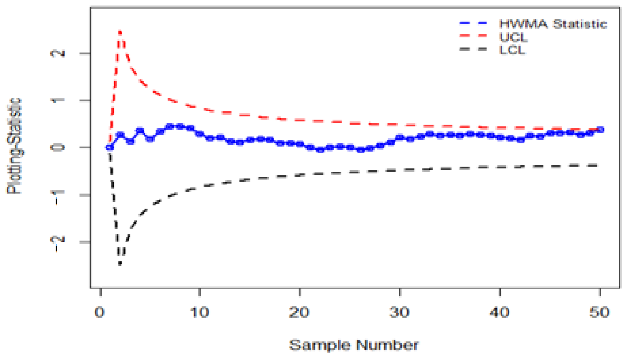
2.1. Design Structure of the HWMA Control Chart

Assume the quality characteristic $Y_{ij}~N(\mu ,{\sigma }^2)$ to be monitored; when the process is IC, it is assumed that both process parameters $\mu$ and $\sigma$ are known, i.e., $\mu ={\mu }_0 \mathrm{and} \sigma ={\sigma }_y$, respectively. To monitor the process mean, the classical HWMA chart was recently designed by Abbas [5]. The plotting statistic of the HWMA chart is given as:

$$H_i=\lambda {\overline{Y}}_i+(1-\lambda ){\overline{\overline{Y}}}_{i-1},$$

(1)

where $\lambda$ is known as smoothing parameter that is parameter of the HWMA charting scheme; its value lies between 0 and 1. The HWMA chart is more efficient at small choices of the smoothing parameter $\lambda$. Abbas [5] showed that the Shewhart control chart becomes the particular case of the HWMA chart at $\lambda$ = 1. Where ${\overline{\overline{Y}}}_{i-1}=\frac{{\displaystyle \sum _{k=1}^{i-1}{\overline{Y}}_k}}{i-1}$ is the mean of the remaining $(i-1)$ sample means, and The ${\overline{Y}}_i$ is the sample average of $i^{th}$ the sample. Control limits of the HWMA are given as:

$$\begin{array}{l}LCL=\left\{\begin{array}{ll}{\mu }_0-L\sqrt{\frac{{\lambda }^2{\sigma }_y^2}{n}},& \mathrm{if} i=1\\ {\mu }_0-L\sqrt{\frac{{\lambda }^2{\sigma }_y^2}{n}+{(1-\lambda )}^2\frac{{\sigma }_y^2}{n(i-1)}},& \mathrm{if} i > 1\end{array}\right.\\ CL={\mu }_0,\\ UCL=\left\{\begin{array}{ll}{\mu }_0+L\sqrt{\frac{{\lambda }^2{\sigma }_y^2}{n}},& \mathrm{if} i=1\\ {\mu }_0+L\sqrt{\frac{{\lambda }^2{\sigma }_y^2}{n}+{(1-\lambda )}^2\frac{{\sigma }_y^2}{n(i-1)}},& \mathrm{if} i > 1\end{array}\right.\end{array}$$

(2)

where the width of the control chart is known as L. The HWMA chart produces an OOC signal if the $H_i$ statistic presented in Equation (1) goes beyond the control limits described in Equation (2).

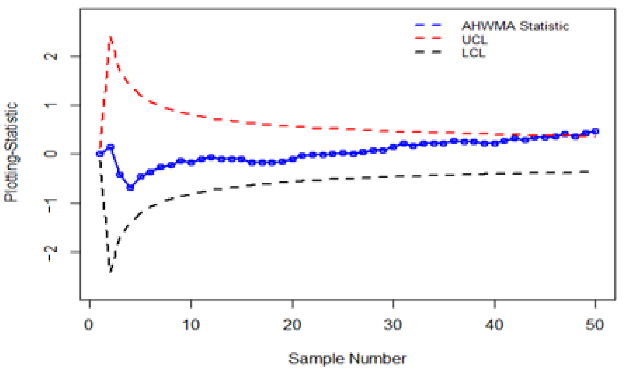
2.2. Design Structure of the AHWMA Control Chart

For monitoring the process location, the supplementary-based HWAM (AHWMA) chart was proposed by Adegoke et al. [20]. According to Adegoke et al. [24], the study variable $Y_{ij}$ is correlated with the supplementary variable $X_{ij}$ (Cochran [25]). The regression can be expressed as:

$$R_i={\overline{Y}}_i+b_{YX}({\mu }_X-{\overline{X}}_i)$$

(3)

where $b_{YX}={\rho }_{YX}\left(\frac{{\sigma }_Y}{{\sigma }_X}\right)$ is expressed as the regression coefficient. The mean and the variance of the regression estimator are ${\mu }_R={\mu }_Y$ and ${\sigma }_R^2=\frac{{\sigma }_Y^2}{n}(1-{\rho }_{YX}^2)$, respectively. The AHWMA charting scheme is given below,

$$D_i=\lambda R_i+(1-\lambda ){\overline{R}}_{i-1}.$$

(4)

In Equation (4) $R_i$ is the regression estimate of the process variable while ${\overline{R}}_{i-1}$ is the average of all previous samples. The control limits of the AHWMA chart are expressed as:

$$\begin{array}{l}LCL=\left\{\begin{array}{ll}{\mu }_0-L{\sigma }_Y\sqrt{\frac{{\lambda }^2}{n}(1-{\rho }_{yx}^2)},& \mathrm{if} i=1\\ {\mu }_0-L{\sigma }_Y\sqrt{(\frac{{\lambda }^2}{n}+\frac{{(1-\lambda )}^2}{n(i-1)})(1-{\rho }_{yx}^2)},& \mathrm{if} i > 1\end{array}\right.\\ CL={\mu }_0,\\ UCL=\left\{\begin{array}{ll}{\mu }_0+L{\sigma }_Y\sqrt{\frac{{\lambda }^2}{n}(1-{\rho }_{yx}^2)},& \mathrm{if} i=1\\ {\mu }_0+L{\sigma }_Y\sqrt{(\frac{{\lambda }^2}{n}+\frac{{(1-\lambda )}^2}{n(i-1)})(1-{\rho }_{yx}^2)},& \mathrm{if} i > 1\end{array}\right.\end{array}$$

(5)

where $L$ is the width of control limits of the AHWMA control chart and $\lambda$ is chosen to achieve a desired IC ARL for the chart. The AHWMA chart produces an OOC signal if the $D_i$ statistic presented in Equation (4) goes outside the control limits given in Equation (5).

2.3. Design Structure of the Classical EWMA Control Chart

The classical EWMA charting scheme to examine the process location was suggested by Roberts [4]. The classical EWMA charting statistic is given below:

$$S_i=\lambda {\overline{Y}}_i+(1-\lambda )S_{i-1},$$

(6)

where $S_{i-1}$ is the information at (i − 1)th time $E(S_i)={\mu }_0$, and $Var(S_i)={\sigma }_{\overline{Y}}^2(\frac{\lambda }{2-\lambda }(1-{(1-\lambda )}^{2i}))$ are the mean and variance for the IC process. The control limits for the classical EWMA charts are:

$$\begin{array}{l}LCL=\left\{{\mu }_0-L{\sigma }_{\overline{Y}}\sqrt{\frac{\lambda }{2-\lambda }(1-{(1-\lambda )}^{2i})},\right.\\ CL={\mu }_0,\\ UCL=\left\{{\mu }_0+L{\sigma }_{\overline{Y}}\sqrt{\frac{\lambda }{2-\lambda }(1-{(1-\lambda )}^{2i})}.\right.\end{array}$$

(7)

It is interesting to note that the Shewhart chart is a special case of EWMA at $\lambda$ = 1. The classical EWMA chart detects an OOC state if any plotting statistic $S_i$ falls beyond the control limits described in Equation (7).

2.4. Design Structure of the AEWMA Control Chart

The supplementary variable-based EWMA chart for monitoring the process location was suggested by Abbas et al. [12]. Let us assume $X_i$ known as a supplementary variable and is associated with the variable of interest $Y_i$. The term ${\rho }_{YX}$ is known as the correlation between the two variables. The bivariate symmetrical distribution can be expressed as $(Y,X)~N_2({\mu }_{Y,}{\mu }_X,{\sigma }_Y^2,{\sigma }_X^2,{\rho }_{YX})$. For monitoring the population mean ${\mu }_0$, the regression estimator based on supplementary information is given as (Cochran [25]):

$$C_Y=\overline{Y}+b_{YX}({\mu }_X-\overline{X}),$$

(8)

where $b_{YX}={\rho }_{YX}\left(\frac{{\sigma }_Y}{{\sigma }_X}\right)$ is presenting change the measures Y due to a one-unit change in X, and in Equation (9) mean and variance of the regression estimator is given below

$$E(C_Y)={\mu }_0,Var(C_Y)={\sigma }_Y^2=\frac{{\sigma }_Y^2}{n}(1-{\rho }_{YX}^2)=\frac{{\sigma }_Y^2-b_{YX}^2{\sigma }_X^2}{n},$$

(9)

$C_Y$ is an unbiased estimator of ${\mu }_0$ and $Var(C_Y)<Var(\overline{Y)}$ for ${\rho }_{YX}^2>0$. The AEWMA statistic based on the regression estimator is defined as

$$E_i=\lambda C_Y+(1-\lambda )E_{i-1}$$

(10)

The value of EWMA statistics $E_{i-1}$ presents past information and is taken from the initial to (i − 1) sample group. The value $E_0$ is commonly accepted as equal to the target mean ${\mu }_0$. The variance $Var(C_Y)={\sigma }_Y^2=\frac{{\sigma }_Y^2}{n}(1-{\rho }_{YX}^2)=\frac{{\sigma }_Y^2-b_{YX}^2{\sigma }_X^2}{n}$ and its means are the target value of the process. The control limits of the AHWMA control chart are given as;

$$\begin{array}{l}LCL=\left\{{\mu }_0-L{\sigma }_Y\sqrt{(1-{\rho }_{YX}^2)(\frac{\lambda }{2-\lambda }(1-{(1-\lambda )}^{2i})),}\right.\\ CL={\mu }_0,\\ ULC=\left\{{\mu }_0+L{\sigma }_Y\sqrt{(1-{\rho }_{YX}^2)(\frac{\lambda }{2-\lambda }(1-{(1-\lambda )}^{2i})).}\right.\end{array}$$

(11)

The AEWMA charting scheme detects OOC if any plotting statistic falls beyond the control limits.

3. Proposed TAHWMA Control Chart

The design structure of the proposed TAHWMA control chart and performance metrics are discussed in this section. The proposed TAHWMA structure is designed under the presence and absence of multicollinearity.

3.1. Design Structure of the Proposed TAHWMA Control Chart

This section of the article provides the detailed design structure of the proposed TAHWMA charting scheme. Here three variables are selected from a trivariate symmetrical distribution such as $Y, X,$ and $Z$. $X$ and $Z$ are the supplementary variables, and $Y$ presents the study variable. The matrix form of the variables is organized below:

$$\left(\begin{array}{l}Y\\ X\\ Z\end{array}\right)~N_3\left(\left(\begin{array}{l}{\mu }_Y\\ {\mu }_X\\ {\mu }_Z\end{array}\right),\left(\begin{array}{l}{\sigma }_{yy}{\sigma }_{yx}{\sigma }_{yz}\\ {\sigma }_{xy}{\sigma }_{xx}{\sigma }_{xz}\\ {\sigma }_{zy}{\sigma }_{zx}{\sigma }_{zz}\end{array}\right)\right)$$

The regression-based estimator initiated by Kadilar and Cingi [26] is given as,

$$G_i=\overline{y}+b_{yx}({\mu }_x-\overline{x})+b_{yz}({\mu }_z-\overline{z}),$$

(12)

where $\left(b_{yx}=\frac{s_{yx}}{s_{xx}}\right)$ and $\left(b_{yz}=\frac{s_{yz}}{s_{zz}}\right)$ are the regression coefficient, $s_{yx}$ and $s_{yz}$ are sample covariances of $Y, X$ and $Y, Z$. While $s_{xx}$ and $s_{zz}$ are the sample variances of $X$ and $Z$, respectively. The mean and variance of Equation (12) are $E(G)={\mu }_G={\mu }_0$ $Var(G)={\sigma }_G^2=(1-{\rho }_{yx}^2-{\rho }_{yz}^2+2{\rho }_{yx}{\rho }_{yz}{\rho }_{xz})\frac{{\sigma }_Y^2}{n}$, respectively (cf. Kadilar and Cingi [27]). The proposed TAHWMA charting scheme based on the regression estimator (in Equation (12)) is given as,

$$H_i=\lambda G_i+(1-\lambda ){\overline{\overline{G}}}_{i-1}$$

(13)

$$\begin{array}{l}LCL=\left\{\begin{array}{ll}{\mu }_0-L\sqrt{\frac{{\lambda }^2{\sigma }_G^2}{n}},& \mathrm{if} i=1\\ {\mu }_0-L\sqrt{\frac{{\lambda }^2{\sigma }_G^2}{n}+{(1-\lambda )}^2\frac{{\sigma }_G^2}{n(i-1)}},& \mathrm{if} i>1\end{array}\right. \\ \mathrm{CL}={\mu }_0,\\ UCL=\left\{\begin{array}{ll}{\mu }_0+L\sqrt{\frac{{\lambda }^2{\sigma }_G^2}{n}}.& \mathrm{if} i=1\\ {\mu }_0+L\sqrt{\frac{{\lambda }^2{\sigma }_G^2}{n}+{(1-\lambda )}^2\frac{{\sigma }_G^2}{n(i-1)}}.& \mathrm{if} i>1\end{array}\right.\end{array}$$

(14)

Control limits of the proposed TAHWMA control chart are presented in Equation (14), where L represents the width of the control limits. Simulation codes are established in R software for the performance evaluation of the proposed chart. The amount of shift in the process mean can be mathematically expressed as $\delta =\frac{\left|{\mu }_1-{\mu }_0\right|}{{\sigma }_y/\sqrt{n}}$, where ${\mu }_1$ denotes the shifted mean of the study variable and n = 1, has taken without loss generality. We use 50,000 iterations in simulation to find the desired average run length. The proposed TAHWMA control chart has two designed parameters $\lambda$, and $L$. $\lambda$ is identified as the smoothing parameter, and the various values of the $\lambda$ is $\lambda \in \{0.03,0.05,0.1,0.25\}$ are considered in this study.

3.2. Performance Metrics

In this section, a detailed discussion of the run length properties of the proposed TAHWMA control chart is carried out using run-length (RL) characteristics. The run length (RL) is defined as the number of sample observations before a chart alarm describes as run-length (RL). Extra quadratic loss (EQL) is also taken as the performance measure of run-length properties, describing the charting schemes’ overall effectiveness. EQL is mathematically defined as $EQL=\frac{1}{{\delta }_{\max }-{\delta }_{\min }}{\displaystyle \underset{{\delta }_{\min }}{\overset{{\delta }_{\max }}{\int }}{\sigma }^{2}ARL(\delta )d\delta }$. Another performance measure is the relative mean index (RMI). Mathematically it is defined as $RMI=\frac{1}{N}{\displaystyle \sum _{i=1}^N\frac{ARL(\delta )-AR{L}^{*}(\delta )}{AR{L}^{*}(\delta )}}$. Where N represents the number of shifts to be considered. For the specific shift $\delta$, $ARL(\delta )$ is the $AR{L}_1$ value of a control chart, while $AR{L}^{*}(\delta )$ represents the smallest value of the $AR{L}_1$. The percentage decrease in ARL is $AR{L}_d$, where $AR{L}_d$ = $\left(\frac{AR{L}_0-AR{L}_1}{AR{L}_0}\right)\times 100\%$. $AR{L}_0$ shows the ARL when the process is working in stable conditions and $AR{L}_1$ presents ARL values when the process is in an OOC situation. For each value of $\lambda$, the $AR{L}_0$ is fixed at 500 using the Monte Carlo simulation method. A comprehensive discussion on the RL distribution of the newly suggested TAHWMA charting scheme is examined under the appearance and non-appearance of the multicollinearity among the two supplementary characteristics.

3.2.1. Performance of the Proposed TAHWMA Control Chart under the Non-Appearance of Multicollinearity

In this section, we examined the performance of the suggested TAHWMA charting scheme under the appearance and non-appearance of multicollinearity among the two supplementary variables. If there is no relationship between the supplementary variable such as ${\rho }_{xz}$ = 0, both supplementary variables have a partial effect on the study variable. Under the appearance of multicollinearity, the ARL values of the suggested TAHWMA charting scheme at several choices of the parameters are given in

Table 1. ARL values of the proposed TAHWMA chart in absence of multicollinearity at various choices of design parameters.

$\mathit{\delta }$	Small Shifts						Moderate Shifts			Large Shifts
	$\mathit{\lambda }$ = 0.03, L = 2.272			$\mathit{\lambda }$ = 0.05, L = 2.608			$\mathit{\lambda }$ = 0.10, L = 2.938			$\mathit{\lambda }$ = 0.25, L = 3.075
	${\mathit{\rho }}_{\mathit{y}\mathit{x}}$ = 0.25	${\mathit{\rho }}_{\mathit{y}\mathit{x}}$ = 0.5	${\mathit{\rho }}_{\mathit{y}\mathit{x}}$ = 0.75	${\mathit{\rho }}_{\mathit{y}\mathit{x}}$ = 0.25	${\mathit{\rho }}_{\mathit{y}\mathit{x}}$ = 0.5	${\mathit{\rho }}_{\mathit{y}\mathit{x}}$ = 0.75	${\mathit{\rho }}_{\mathit{y}\mathit{x}}$ = 0.25	${\mathit{\rho }}_{\mathit{y}\mathit{x}}$ = 0.5	${\mathit{\rho }}_{\mathit{y}\mathit{x}}$ = 0.75	${\mathit{\rho }}_{\mathit{y}\mathit{x}}$ = 0.25	${\mathit{\rho }}_{\mathit{y}\mathit{x}}$ = 0.5	${\mathit{\rho }}_{\mathit{y}\mathit{x}}$ = 0.75
	${\mathit{\rho }}_{\mathit{y}\mathit{z}}$ = 0.50, ${\mathit{\rho }}_{\mathit{x}\mathit{z}}$ = 0			${\mathit{\rho }}_{\mathit{y}\mathit{z}}$ = 0.50, ${\mathit{\rho }}_{\mathit{x}\mathit{z}}$ = 0			${\mathit{\rho }}_{\mathit{y}\mathit{z}}$ = 0.50, ${\mathit{\rho }}_{\mathit{x}\mathit{z}}$ = 0			${\mathit{\rho }}_{\mathit{y}\mathit{z}}$ = 0.50, ${\mathit{\rho }}_{\mathit{x}\mathit{z}}$ = 0
0	499.92	500.59	500.50	500.87	500.48	500.00	499.70	499.68	500.22	500.96	499.81	500.92
0.03	422.12	393.17	291.19	432.70	408.11	315.37	439.43	421.68	335.05	466.80	455.76	398.38
0.05	330.14	288.40	174.72	345.68	310.76	194.21	362.74	330.82	218.70	419.96	392.24	290.20
0.075	226.50	193.27	104.73	254.06	217.28	120.66	272.73	237.35	136.16	346.73	310.04	189.49
0.1	165.07	136.69	69.23	186.99	157.06	81.87	208.11	173.65	91.86	274.62	239.11	127.87
0.125	125.40	100.83	48.69	144.15	118.10	59.37	160.82	132.53	66.29	223.38	184.65	89.11
0.175	79.36	62.04	28.51	92.93	74.41	35.17	103.92	83.45	39.74	145.17	114.72	50.07
0.2	64.22	50.32	22.92	76.32	60.70	28.69	85.96	68.58	32.40	117.87	92.28	39.13
0.25	45.82	35.69	15.80	55.40	43.76	19.81	62.29	48.84	22.81	82.98	63.02	26.01
0.5	14.74	11.35	5.34	18.53	14.13	6.48	21.19	16.43	7.44	24.20	18.19	7.52
0.75	7.69	6.09	3.08	9.40	7.33	3.61	11.02	8.57	4.08	11.53	8.76	3.95
1	5.01	4.02	2.11	6.00	4.75	2.46	6.88	5.44	2.71	7.09	5.44	2.61
1.5	2.89	2.36	1.21	3.40	2.76	1.35	3.81	3.08	1.50	3.68	2.93	1.45
2	1.97	1.58	1.02	2.31	1.84	1.03	2.58	2.07	1.06	2.44	1.95	1.06

. For tracing the small shift in the process mean, it is obvious that small choices of smoothing parameter, high values of the ${\mathsf{\rho }}_{\mathrm{YX} }$ and ${\mathsf{\rho }}_{\mathrm{YZ} }$, and the suggested TAHWMA charting scheme becomes more sensitive. The suggested TAHWMA charting scheme with designed parameters $\lambda$ = 0.03, $L$ = 2.272, ${\mathsf{\rho }}_{\mathrm{YX} }$= 0.25 and ${\mathsf{\rho }}_{\mathrm{YZ}}=0.50$, provides ${\mathrm{ARL}}_1$ = 330.14 and $AR{L}_d$ = 33.97% at $\delta$ = 0.05. At $\lambda$ = 0.03, $L$ = 2.272, ${\mathsf{\rho }}_{\mathrm{YX} }$= 0.75 and ${\mathsf{\rho }}_{\mathrm{YZ}}=0.50$, at 3% increase in the process mean the suggested TAHWMA charting scheme yields $AR{L}_d$ = 65.05% (see Table 1). The effect of the ${\mathsf{\rho }}_{\mathrm{YX} }$ and ${\mathsf{\rho }}_{\mathrm{YZ}}$ on the performance of the proposed TAHWMA model can be seen in Figure 1 and Figure 2. From Figure 1 and Figure 2, it can be observed that the values of ${\mathsf{\rho }}_{\mathrm{YX} }$ and ${\mathsf{\rho }}_{\mathrm{YZ}}$ increase, and the performance of the suggested TAHWMA charting scheme also becomes highly sensitive.

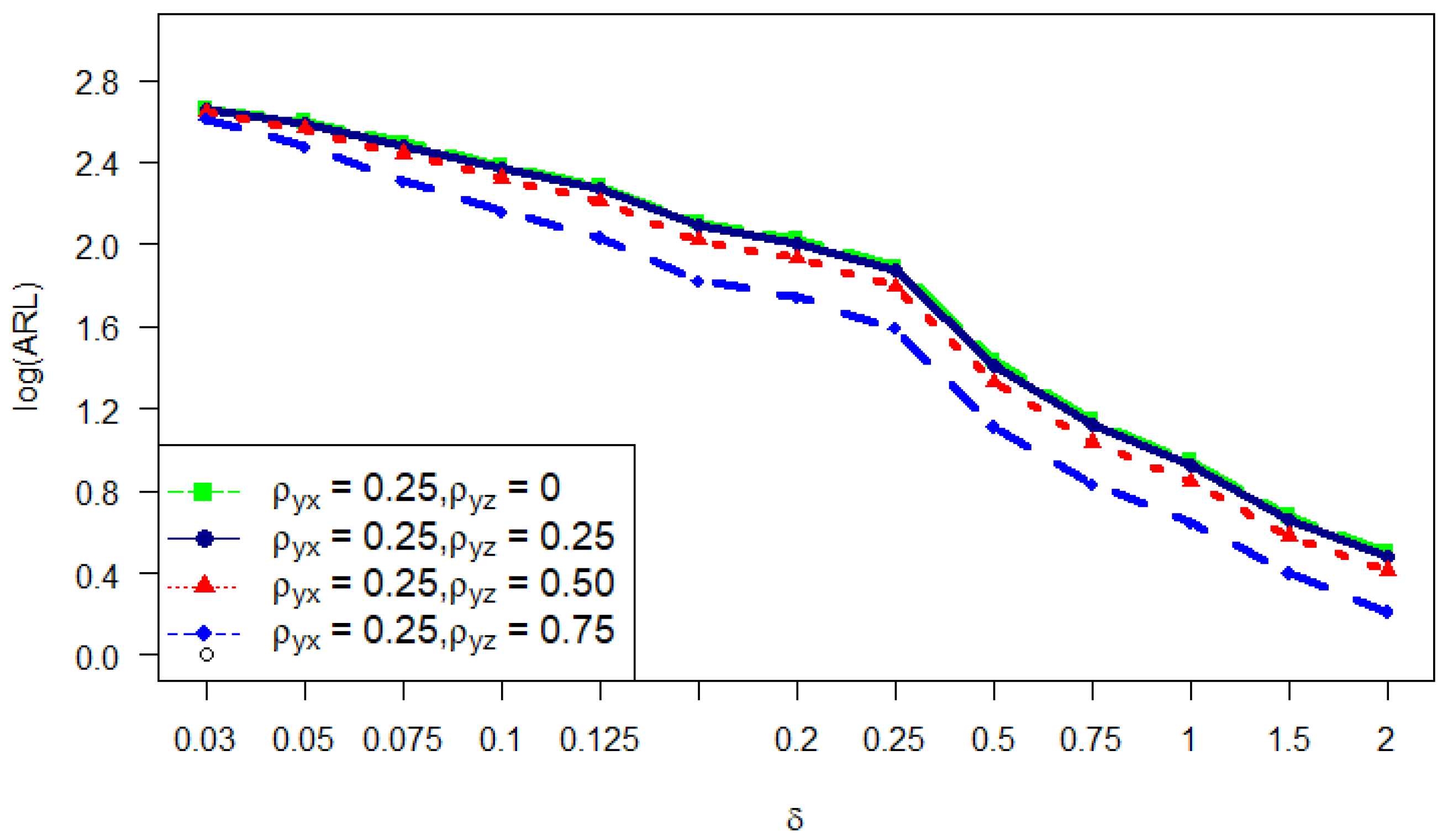
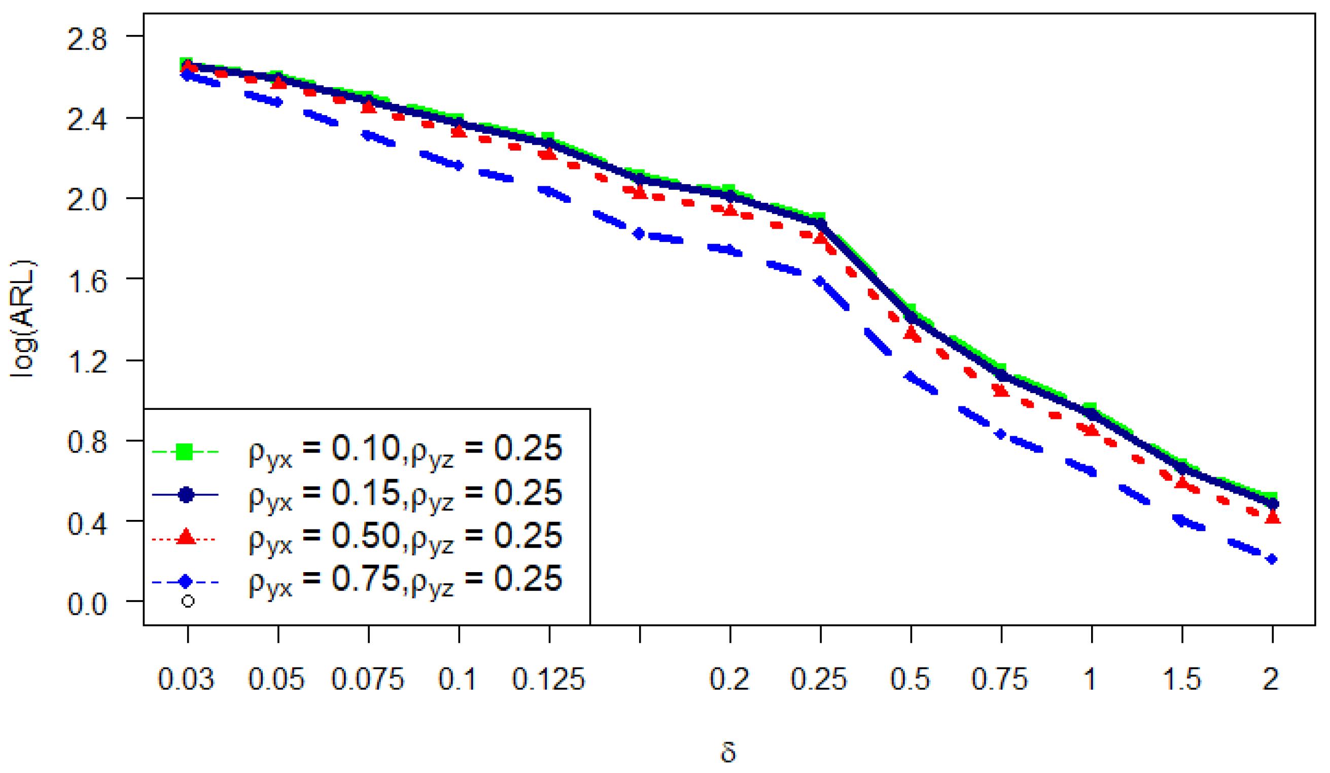
3.2.2. Performance of the Proposed TAHWMA Control Chart under the Appearance of Multicollinearity

If some linear relationship occurs between the two supplementary variables, this term is expressed as multicollinearity (cf. Hocking and Pendleton [26]). Unfortunately, multicollinearity happens due to mistakes or a lack of understanding of the model. It is vital to know about the effect of multicollinearity between two supplementary variables on the performance of the suggested TAHWMA charting scheme. The performance of the suggested TAHWMA charting scheme is reported at various choices of correlation between two supplementary characteristics, i.e., ${\rho }_{xz}$ $\in$ 0.05, 0.15, and 0.25 (cf.

Table 2. ARL values of proposed TAHWMA control chart under the presence of multicollinearity when ${\rho }_{yx}$ = 0.25 and ${\rho }_{yz}$ = 0.50.

$\mathit{\delta }$	${\mathit{\rho }}_{\mathit{x}\mathit{z}}$ = 0.05			${\mathit{\rho }}_{\mathit{x}\mathit{z}}$ = 0.15			${\mathit{\rho }}_{\mathit{x}\mathit{z}}$ = 0.25
	$\mathit{\lambda }$ = 0.05, $\mathit{L}$ = 2.633			$\mathit{\lambda }$ = 0.05, $\mathit{L}$ = 2.679			$\mathit{\lambda }$ = 0.05, $\mathit{L}$ = 2.719
	ARL	SDRL	MDRL	ARL	SDRL	MDRL	ARL	SDRL	MDRL
0	501.18	372.02	438	499.75	372.26	437	495.53	368.77	436
0.03	434.94	329.12	376	434.31	331.05	373	429.45	329.72	367
0.05	349.49	274.23	291	353.02	278.69	295	354.30	279.99	294
0.075	253.89	200.40	210	261.87	204.59	216	262.13	205.74	218
0.1	190.50	147.65	160	192.57	150.72	161	196.71	154.48	164
0.125	145.68	110.16	123	150.41	114.68	127	151.95	116.03	127
0.175	94.24	69.61	81	96.52	71.67	82	98.10	73.09	83
0.2	78.06	56.57	67	79.25	57.85	68	81.47	59.95	69
0.25	56.42	40.24	49	57.62	41.41	50	58.68	41.95	51
0.5	18.59	12.44	16	19.24	12.93	17	19.58	13.27	17
0.75	9.53	5.95	8	9.87	6.20	9	10.08	6.33	9
1	6.17	3.49	6	6.23	3.51	6	6.41	3.67	6
1.5	3.44	1.74	3	3.52	1.77	3	3.60	1.85	3
2	2.34	1.26	3	2.40	1.28	3	2.44	1.31	3

). In Table 2, it can be noticed that as the value ${\rho }_{xz}$ increases, the performance of the suggested TAEWMA charting structure decreases. For example, at $\lambda$ = 0.05, $L$ = 2.633 and ${\rho }_{xz}$ = 0.05 at $\delta$ = 0.05, the proposed scheme provides $AR{L}_1$ = 349.49 and at ${\rho }_{xz}$ = 0.25, $\lambda$ = 0.05 it gives $AR{L}_1$ = 354.30 respectively (cf. Table 2).

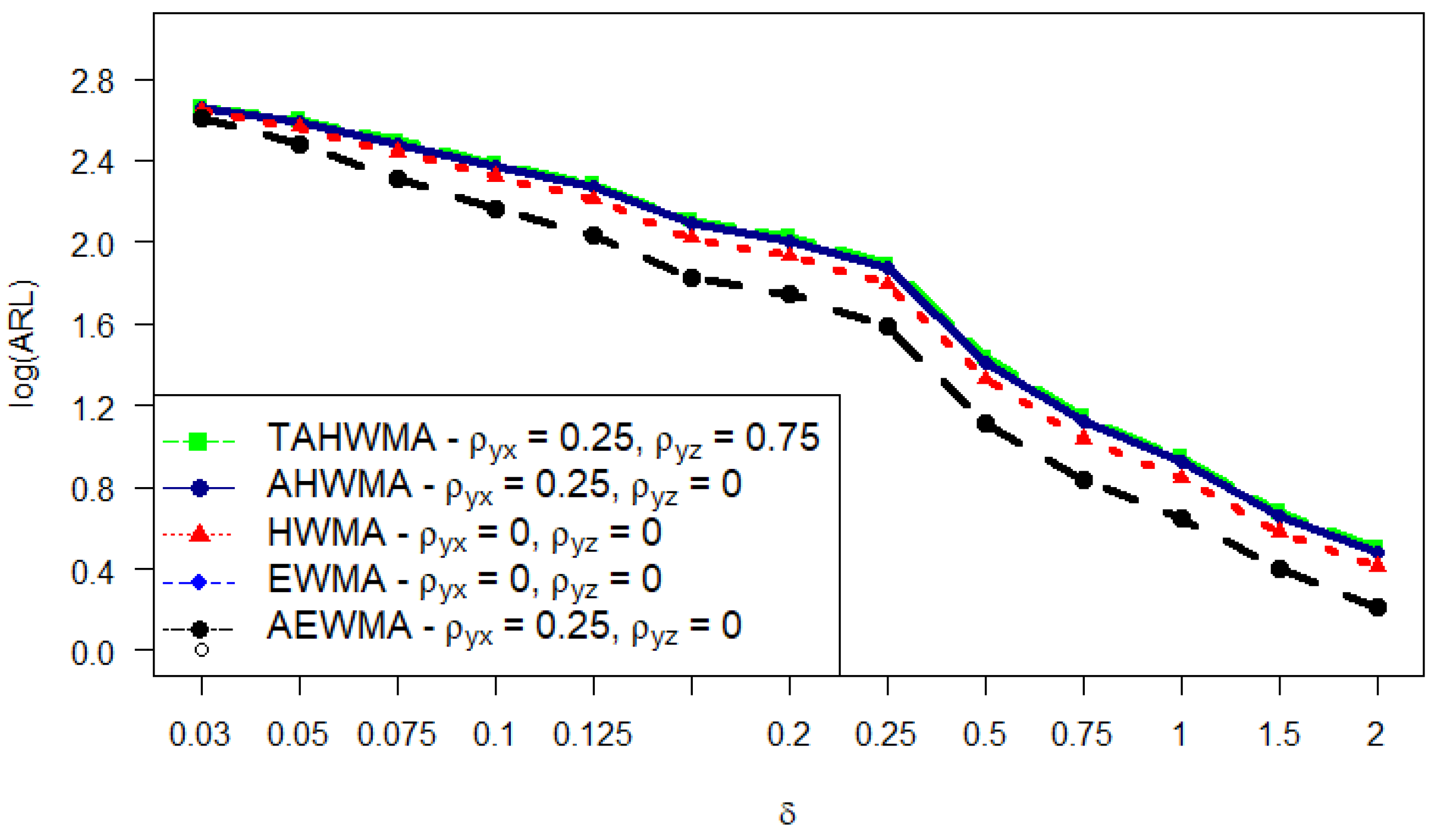
4. Comparative Study

In this section, a comparison of the proposed TAHWMA chart is provided against some existing control charts. The ARL is a comparative index for classical EWMA, AEWMA, HWMA, AHWMA, and proposed TAHWMA charts.

4.1. Proposed Versus EWMA and AEWMA Control Charts

The classical EWMA charting scheme is famous for examining the small shifts in the process; the classical EWMA chart was initiated by Roberts [4]. Abbas et al. [12] suggested a new charting scheme, AEWMA, for the efficient monitoring of the process mean. In

Table 3. The ARL values of the EWMA and AEWMA control charts.

$\mathit{\delta }$	EWMA				AEWMA (${\mathit{\rho }}_{\mathit{y}\mathit{x}}$ = 0.25)
	$\mathit{\lambda }$ = 0.03 $\mathit{L}$ = 2.483	$\mathit{\lambda }$ = 0.05 $\mathit{L}$ = 2.639	$\mathit{\lambda }$ = 0.1 $\mathit{L}$ = 2.824	$\mathit{\lambda }$ = 0.25 $\mathit{L}$ = 3.001	$\mathit{\lambda }$ = 0.03 $\mathit{L}$ = 2.483	$\mathit{\lambda }$ = 0.05 $\mathit{L}$ = 2.639	$\mathit{\lambda }$ = 0.1 $\mathit{L}$ = 2.824	$\mathit{\lambda }$ = 0.25 $\mathit{L}$ = 3.001
0	500.64	499.68	500.94	499.79	500.33	500.36	500.39	500.78
0.03	456.41	462.91	480.81	488.19	453.72	466.58	475.58	484.32
0.05	388.18	412.31	438.70	466.30	382.72	408.43	438.29	462.55
0.075	304.78	338.65	376.08	435.67	301.97	328.86	372.44	427.63
0.1	232.24	266.78	318.91	390.56	229.75	262.54	314.47	384.82
0.125	181.85	211.65	264.66	346.91	177.55	202.55	251.93	336.03
0.175	113.49	135.20	177.02	262.29	110.97	130.36	168.29	254.75
0.2	93.56	111.53	148.70	224.77	90.34	106.50	139.50	219.07
0.25	67.29	76.75	102.97	169.33	63.26	73.58	97.39	161.22
0.5	21.19	23.74	29.12	47.85	20.25	22.26	26.81	44.31
0.75	10.77	11.93	13.58	19.27	10.14	11.18	12.78	18.02
1	6.60	7.40	8.25	10.38	6.34	6.92	7.71	9.76
1.5	3.42	3.77	4.17	4.79	3.29	3.59	3.98	4.49
2	2.25	2.41	2.65	2.93	2.15	2.31	2.52	2.80

, ARL values of both existing charting schemes such as classical EWMA and AEWMA are described. At $\lambda$ = 0.05 and $\delta$ = 0.075 classical EWMA yields $AR{L}_1$ = 338.65 and for AEWMA at $\lambda$ = 0.05 and $\delta$ = 0.075 ${\rho }_{yx}$ = 0.25, $AR{L}_1$ = 328.86 respectively. The proposed TAHWMA chart at $\lambda$ = 0.05, $\delta$ = 0.075, ${\rho }_{yx}$ = 0.25 and ${\rho }_{yz}$ = 0.50 produces $AR{L}_1$ = 254.06, respectively (cf. Table 1). From Table 1 and Table 3, we noticed that the suggested TAHWMA charting scheme performs more efficiently than AEWMA and classical EWMA charting schemes to detect small and moderate shifts in the process mean level.

4.2. Proposed Versus HWMA and AHWMA Control Charts

The HWMA scheme was recently developed by Abbas [5] to address small changes in the process mean. To increase the sensitivity of the HWMA model, Adegoke et al. [24] designed the AHWMA chart using a regression estimator that is based on the single supplementary variable. The values of ARL for both classical HWMA and AHWMA control charts are given in

Table 4. The ARL values of the HWMA and AHWMA control charts.

$\mathit{\delta }$	HWMA				AHWMA ( ${\mathit{\rho }}_{\mathit{y}\mathit{x}}$ = 0.25)
	$\mathit{\lambda }$ = 0.03 $\mathit{L}$ = 2.272	$\mathit{\lambda }$ = 0.05 $\mathit{L}$ = 2.608	$\mathit{\lambda }$ = 0.1 $\mathit{L}$ = 2.938	$\mathit{\lambda }$ = 0.25 $\mathit{L}$ = 3.075	$\mathit{\lambda }$ = 0.03 $\mathit{L}$ = 2.272	$\mathit{\lambda }$ = 0.05 $\mathit{L}$ = 2.608	$\mathit{\lambda }$ = 0.1 $\mathit{L}$ = 2.938	$\mathit{\lambda }$ = 0.25 $\mathit{L}$ = 3.075
0	500.70	499.35	499.48	499.69	499.98	500.18	500.96	500.34
0.03	440.12	449.24	456.35	473.57	442.47	448.12	453.61	473.88
0.05	359.03	382.47	397.11	441.31	359.39	380.54	393.94	445.27
0.075	274.16	298.00	313.35	382.72	266.64	286.42	310.21	377.80
0.1	205.43	229.66	250.83	329.77	199.38	222.00	242.77	317.69
0.125	158.89	179.95	201.22	270.99	151.54	174.35	191.82	265.10
0.175	101.43	119.55	133.63	187.62	97.86	115.19	127.79	179.99
0.2	84.52	99.66	111.81	158.76	80.32	96.17	106.49	148.73
0.25	61.19	73.06	81.59	113.01	58.59	69.15	78.16	106.86
0.5	20.08	25.26	28.57	33.96	19.09	23.76	27.27	31.84
0.75	10.36	12.80	14.89	16.12	9.82	12.25	14.07	15.24
1	6.64	7.99	9.37	9.74	6.28	7.63	8.81	9.14
1.5	3.72	4.41	4.97	4.92	3.56	4.22	4.75	4.66
2	2.55	3.00	3.33	3.18	2.44	2.85	3.18	3.05

at various combinations of designed parameters. For example, At $\lambda$ = 0.03 the classical HWMA scheme yields $AR{L}_1$ = 205.43 at $\delta$ = 0.1. For the AHWMA chart, at ${\rho }_{yx}$ = 0.25, $\lambda$ = 0.3 and $\delta$ = 0.1, the value of $AR{L}_1$ = 199.38 (cf. Table 4). The suggested TAHWMA charting scheme at $\lambda$ = 0.03, $\delta$ = 0.1 and ${\rho }_{yx}$ = 0.25 and ${\rho }_{yz}$ = 0.50 yields $AR{L}_1$ = 165.07 (cf. Table 1). The supremacy of the suggested TAHWMA charting scheme is obvious over the classical HWMA and AHWMA schemes (cf. Table 1 and Table 4).

In

Table 5. ARL comparisons of the proposed TAHWMA and the existing control chart.

	TAHWMA				EWMA	AEWMA	HWMA	AHWMA
Shift	$\mathit{\lambda }$ = 0.03	$\mathit{\lambda }$ = 0.05	$\mathit{\lambda }$ = 0.1	$\mathit{\lambda }$ = 0.25	$\mathit{\lambda }$ = 0.03	$\mathit{\lambda }$ = 0.03	$\mathit{\lambda }$ = 0.03	$\mathit{\lambda }$ = 0.03
0	500.5	500	500.22	500.92	500.64	500.33	500.7	499.98
0.03	291.19	315.37	335.05	398.38	456.41	453.72	440.12	442.47
0.05	174.72	194.21	218.7	290.2	388.18	382.72	359.03	359.39
0.075	104.73	120.66	136.16	189.49	304.78	301.97	274.16	266.64
0.1	69.23	81.87	91.86	127.87	232.24	229.75	205.43	199.38
0.125	48.69	59.37	66.29	89.11	181.85	177.55	158.89	151.54
0.175	28.51	35.17	39.74	50.07	113.49	110.97	101.43	97.86
0.2	22.92	28.69	32.4	39.13	93.56	90.34	84.52	80.32
0.25	15.8	19.81	22.81	26.01	67.29	63.26	61.19	58.59
0.5	5.34	6.48	7.44	7.52	21.19	20.25	20.08	19.09
0.75	3.08	3.61	4.08	3.95	10.77	10.14	10.36	9.82
1	2.11	2.46	2.71	2.61	6.6	6.34	6.64	6.28
1.5	1.21	1.35	1.5	1.45	3.42	3.29	3.72	3.56
2	1.02	1.03	1.06	1.06	2.25	2.15	2.55	2.44
EQL	2.12	2.37	2.61	2.60	6.28	6.01	6.48	6.18
RMI	0.00	0.17	0.30	0.52	2.21	2.10	2.03	1.91

, the relative mean index (RMI) and extra quadratic loss (EQL) are also considered performance measures. For the proposed TAHWMA control chart $\lambda \in (0.03,0.05,0.1,0.25)$ is used when ${\rho }_{yx}$ = 0.75, ${\rho }_{yz}$ = 0.50, and ${\rho }_{xz}$ = 0. Other existing charting schemes such as HWMA, EWMA, AEWMA, and AHWMA are also considered when $\lambda$ = 0.03. For the proposed TAHWMA chart, when $\lambda$ = 0.03, RMI has a minimum value of zero and the proposed TAHWMA chart also has the minimum value of the EQL, which is 2.12. The minimum values of the RMI and EQL show the supremacy of the suggested TAHWMA charting scheme against its existing charting structure.

In Figure 3, the supremacy of the proposed TAHWMA charting structure (in terms of smallest ARL₁) is evident compared to all the competitors at small, moderate and large shifts in the process mean. The performance of the AHWMA scheme is the second best.

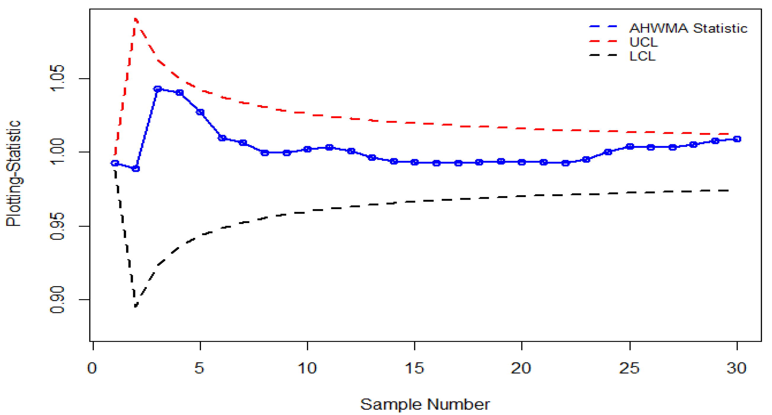
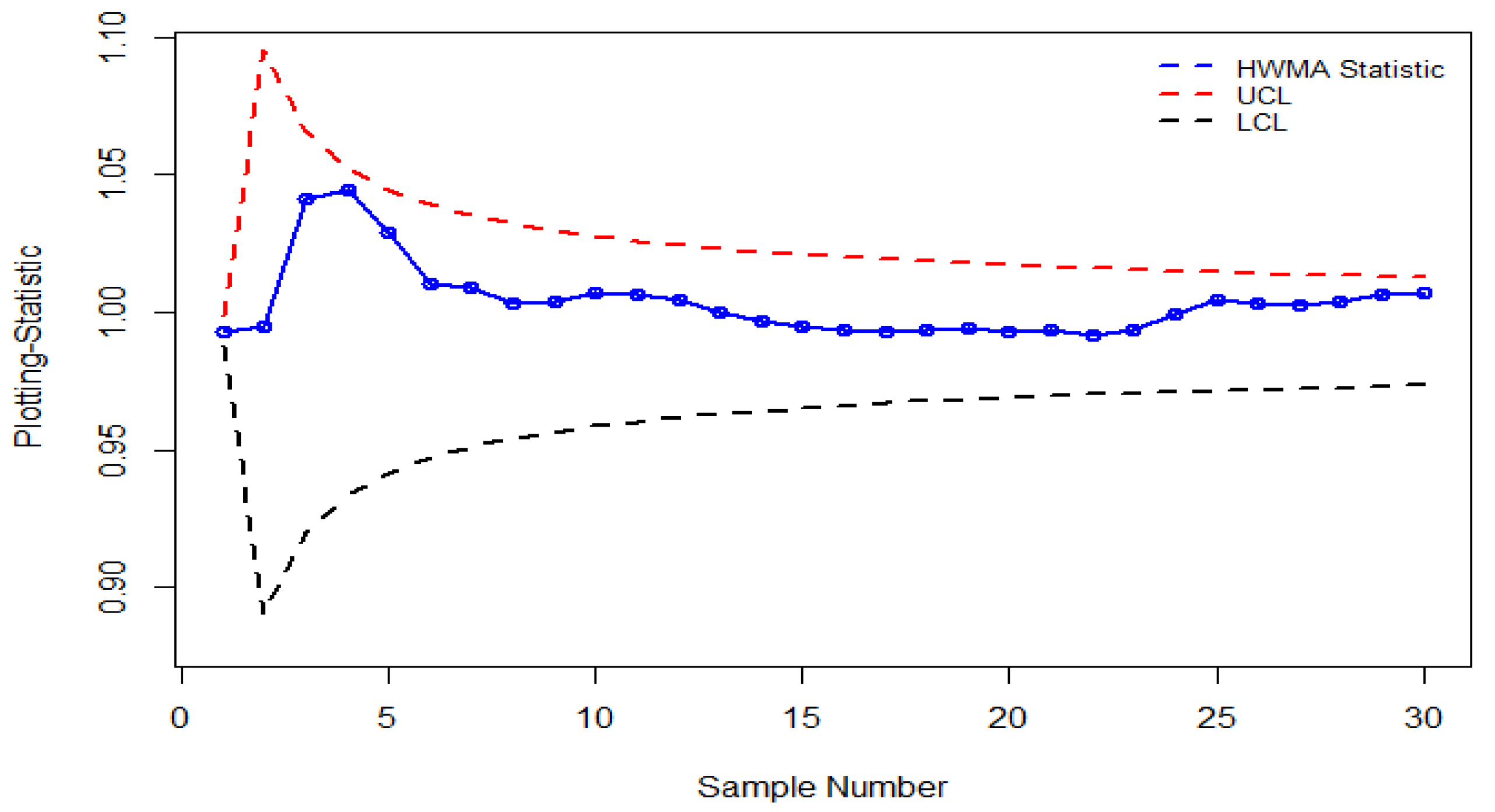
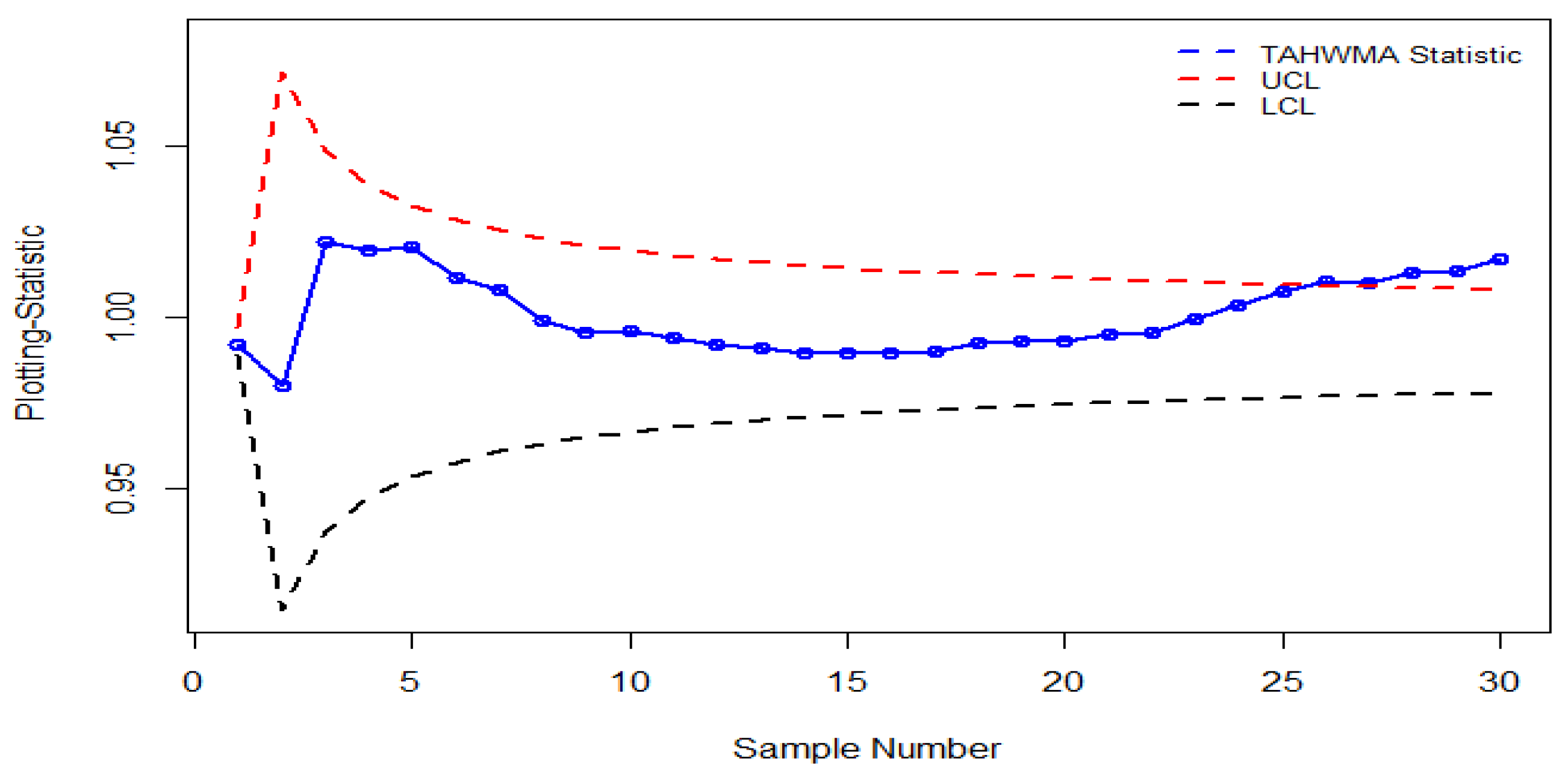
5. Illustrative Example

Along with exploring the several properties of the suggested TAHWMA charting scheme hypothetically, it is necessary to offer an illustrative example of the developed design. Two examples are presented in this section to show the supremacy of the proposed TAHWMA chart; one consists of the real dataset and the second is based on simulated data. The first real dataset belongs to the carbon fibre tube (manufacturing data), and the second dataset is taken from the trivariate normal distribution.

5.1. Real-Life Application

In this section, a real dataset example related to manufacturing carbon fibre (graphite fibre) tubes is used to show the application of the proposed TAWHMA chart and its competitors. This carbon dataset is used from the R statistical package “MSQC” and is also used by Abbasi and Adegoke [28]. Carbon fibre tubes are frequently comprised of carbon atoms. It has numerous assets for illustration, high tensile strength, low weight, etc. (cf. Zhang et al. [29]). It is a polymer that is solid but lightweight. It is used to manufacture aircraft, cars, and many other machinery parts. Carbon fibre is produced from polyacrylonitrile (PAN) and a small quantity of petroleum pitch. Carbon fibre is much stronger than steel; it is a fibre having many characteristics, and the size of the fibre is nearly equal to 5 to 10 micrometres. It is low-density material but has high-temperature tolerance, high chemical resistance, high stiffness, and high tensile strength.

In this analysis, $Y$ represents the inner diameter, $X$ represents thickness, and $Z$ represents length. These are the first and second supplementary variables, respectively. These variables belong to the manufacturing process of the fiber tubes. A dataset has 30 samples, where 10 samples are taken with 0.05 amount of shift in the process mean, and 20 samples are taken as the IC process. For the execution of the proposed TAHWMA plotting scheme and prevailing schemes, planned parameters are set at the desired value of ARL = 500 for all the charts included in this example. Some descriptive statistics of the carbon fibre data of the first 20 samples are; $\overline{X}$ is 1.022, and $\overline{Z}$ is 50.1005 and $\overline{Y}$ is 0.993. where $s_y^2$ = 0.001706316, $s_x^2$ = 0.01139579, $s_z^2$ = 0.05572079, ${\rho }_{yx}$ = 0.2778609, ${\rho }_{yz}$ = 0.617334, ${\rho }_{xz}$ = 0.1219354. Figure 4 and Figure 5 show that the HWMA and AHWMA charts are not detecting a 0.05 amount of shift at any sample, whereas the proposed TAHWMA charting structure drops this change at the 25th to 30th sample observations (cf. Figure 6).

In detecting the small changes in the process mean compared to its counterparts, the real-life application indicates that the suggested TAHWMA charting structure is the most powerful tool.

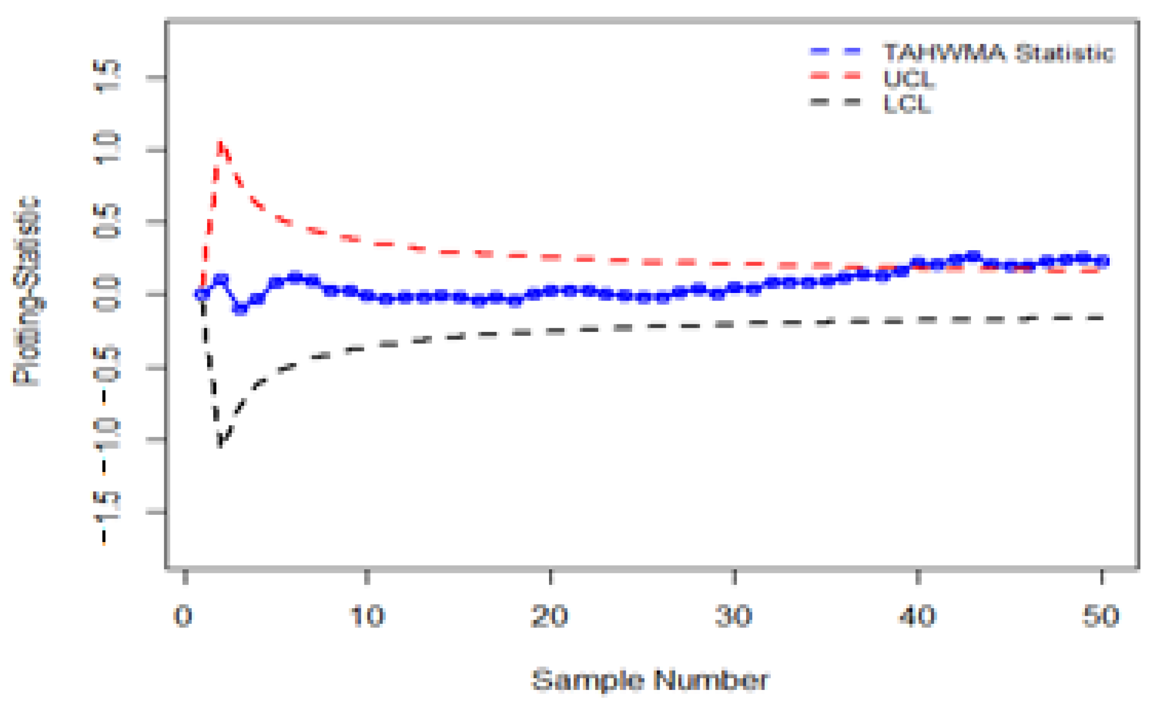
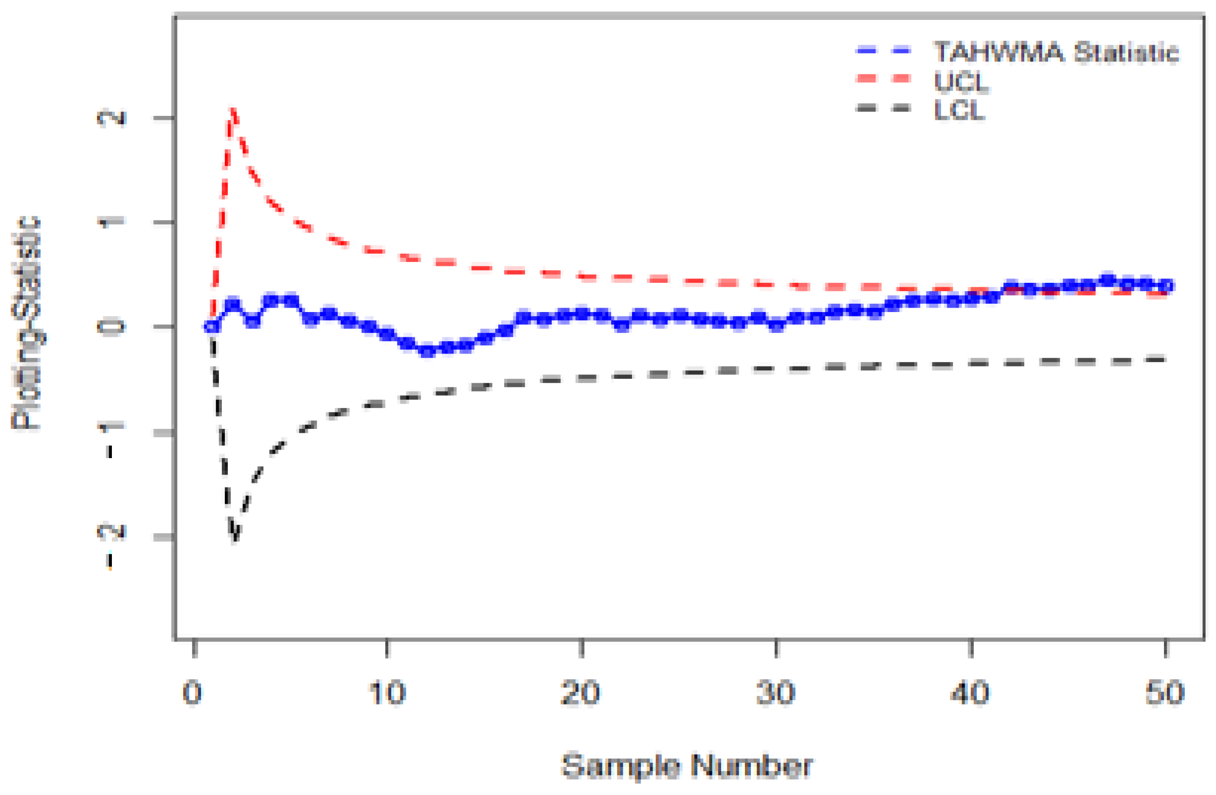
5.2. Simulation Study

This section describes the application using the hypothetical dataset to implement the planned design. In this simulated part of the study, the dataset consists of 50 samples. These 50 samples belong to trivariate symmetrical distribution; for the IC process, 25 samples are considered, and 25 samples are incorporated with a shift of 0.5 in the process mean for the OOC process. The execution of the recommended charting structure is executed considering the appearance and non-appearance of multicollinearity among the two supplementary variables. Further details on the selection of designed parameters for the proposed and existing counterparts are given in Figure 7, Figure 8, Figure 9 and Figure 10. From Figure 7, Figure 8, Figure 9 and Figure 10, it can be observed that all the charts remain in the IC situation for the first 25 samples. In Figure 7, the application of the proposed TAHWMA chart is provided when there is no multicollinearity between the supplementary variables, and it traces a shift at the 39th samples. In Figure 8, the presentation of the proposed TAHWMA control chart is delivered when multicollinearity exists between the supplementary variables. The proposed TAHWMA chart traces the shift at the 41st samples in this case. In Figure 9, the existing chart, namely the HWMA chart, outlines the shift at the 49th samples. In Figure 10, the existing chart, namely the AHWMA chart, detects the shift at 49th samples. Based on the discussion, it is observed that the proposed TAHWMA charting scheme has performed efficiently against existing charting schemes, particularly in the non-appearance of multicollinearity among the two supplementary variables.

6. Summary, Conclusions and Recommendations

The single supplementary information-based (AIB) homogeneously weighted moving (HWMA) chart is an innovative version of the HWMA charting scheme to monitor the process mean shift. This study aims to enhance the HWMA and AIB HWMA charts and propose an HWMA chart based on two supplementary variables, indicated as the TAHWMA charting scheme, to improve the process mean shift monitoring. The run-length characteristic of the proposed TAHWMA charting scheme has been discussed in the absence and presence of multicollinearity between the two supplementary variables. It has been observed that the proposed structure performs better for various correlation coefficient choices, particularly when both supplementary variables consume a fractional effect on the study variable.

To evaluate the performance of the proposed TAHWMA chart against other control existing charts, an algorithm is developed in R software using the Monte Carlo simulation technique to obtain numerical results. Based on numerical results, performance evaluation measures such as ARL, EQL, and RMI are calculated. The analysis based on performance evaluation measures and visual presentation reveals that the proposed charting scheme outperformed existing counterparts. Furthermore, two illustrative examples, one related to the hypothetical dataset and another with regard to a Carbon fibre tube (manufacturing process), are also provided to show the practical implementation of the proposed charting scheme. The proposed charting scheme can be extended for multivariate structures to monitor the process location, dispersion, or both parameters.

References

1. Montgomery, D.C. Introduction to Statistical Quality Control, 7th ed.; John Wiley & Sons: New York, NY, USA, 2012. [Google Scholar]
2. Shewhart, W.A. Quality control charts. Bell Syst. Tech. J. 1926, 5, 593–603. [Google Scholar] [CrossRef]
3. Page, E.S. Continuous inspection schemes. Biometrika 1954, 41, 100–115. [Google Scholar] [CrossRef]
4. Roberts, S. Control chart tests based on geometric moving averages. Technometrics 1959, 1, 239–250. [Google Scholar] [CrossRef]
5. Abbas, N. Homogeneously weighted moving average control chart with an application in substrate manufacturing process. Comput. Ind. Eng. 2018, 120, 460–470. [Google Scholar] [CrossRef]
6. Haq, A.; Khoo, M.B.C. A new double sampling control chart for monitoring process mean using auxiliary information. J. Stat. Comput. Simul. 2017, 88, 869–899. [Google Scholar] [CrossRef]
7. Mandel, B. The regression control chart. J. Qual. Technol. 1969, 1, 1–9. [Google Scholar] [CrossRef]
8. Zhang, G. Cause-selecting control charts—A new type of quality control charts. QR J. 1985, 12, 221–225. [Google Scholar]
9. Riaz, M. Monitoring process mean level using auxiliary information. Stat. Neerl. 2008, 62, 458–481. [Google Scholar] [CrossRef]
10. Riaz, M. Monitoring process variability using auxiliary information. Comput. Stat. 2008, 23, 253–276. [Google Scholar] [CrossRef]
11. Riaz, M.; Mehmood, R.; Ahmad, S.; Abbasi, S.A. On the Performance of Auxiliary-based Control Charting under Normality and Nonnormality with Estimation Effects. Qual. Reliab. Eng. Int. 2013, 29, 1165–1179. [Google Scholar] [CrossRef]
12. Nuriman, M.A.; Mashuri, M.; Ahsan, M. Auxiliary information based generally weighted moving coefficient of variation (AIB-GWMCV) control chart. IOP Conf. Ser. Mater. Sci. Eng. 2021, 1115, 012033. [Google Scholar] [CrossRef]
13. Haq, A.; Khoo, M.B.C. A new synthetic control chart for monitoring process mean using auxiliary information. J. Stat. Comput. Simul. 2016, 86, 3068–3092. [Google Scholar] [CrossRef]
14. Abbasi, S.A. Efficient Control Charts for Monitoring Process CV Using Auxiliary Information. IEEE Access 2020, 8, 46176–46192. [Google Scholar] [CrossRef]
15. Arslan, M.; Ashraf, M.A.; Anwar, S.M.; Rasheed, Z.; Hu, X.; Abbasi, S.A. Novel Mixed EWMA Dual-Crosier CUSUM Mean Charts without and with Auxiliary Information. Math. Probl. Eng. 2022, 1362193. [Google Scholar] [CrossRef]
16. Abbas, Z.; Nazir, H.Z.; Akhtar, N.; Riaz, M.; Abid, M. On designing a progressive mean chart for efficient monitoring of process location. Qual. Reliab. Eng. Int. 2020, 36, 1716–1730. [Google Scholar] [CrossRef]
17. Chen, J.H.; Lu, S.L. A New Sum of Squares Exponentially Weighted Moving Average Control Chart Using Auxiliary In-formation. Symmetry 2020, 12, 1888. [Google Scholar] [CrossRef]
18. Rasheed, Z.; Zhang, H.; Anwar, S.M.; Zaman, B. Homogeneously Mixed Memory Charts with Application in the Substrate Production Process. Math. Probl. Eng. 2021, 2021, 2582210. [Google Scholar] [CrossRef]
19. Aslam, M.; Anwar, S.M.; Khan, M.; Abiodun, N.L.; Rasheed, Z. Efficient Auxiliary Information–Based Control Charting Schemes for the Process Dispersion with Application of Glass Manufacturing Industry. Math. Probl. Eng. 2022, 1265204. [Google Scholar] [CrossRef]
20. Anwar, S.M.; Aslam, M.; Zaman, B.; Riaz, M. Mixed memory control chart based on auxiliary information for simultaneously monitoring of process parameters: An application in glass field. Comput. Ind. Eng. 2021, 156, 107284. [Google Scholar] [CrossRef]
21. Rasheed, Z.; Khan, M.; Abiodun, N.L.; Anwar, S.M.; Khalaf, G.; Abbasi, S.A. Improved Nonparametric Control Chart Based on Ranked Set Sampling with Application of Chemical Data Modelling. Math. Probl. Eng. 2022, 7350204. [Google Scholar] [CrossRef]
22. Zhang, H.; Rasheed, Z.; Khan, M.; Namangale, J.J.; Anwar, S.M.; Hamid, A. A Distribution-Free THWMA Control Chart under Ranked Set Sampling. Math. Probl. Eng. 2022, 2022, 3823013. [Google Scholar] [CrossRef]
23. Zichuan, M.; Arslana, M.; Abbasb, Z.; Abbasic, S.A.; Zafar, H. Improving the Performance of EWMA mean chart using Two Auxiliary Variables. Rev. Argent. Clin. Psicol. 2020, 29, 2016–2024. [Google Scholar]
24. Adegoke, N.A.; Smith, A.N.H.; Anderson, M.J.; Sanusi, R.A.; Pawley, M.D.M. Efficient Homogeneously Weighted Moving Average Chart for Monitoring Process Mean Using an Auxiliary Variable. IEEE Access 2019, 7, 94021–94032. [Google Scholar] [CrossRef]
25. Cochran, W.G. Sampling Techniques, 3rd ed.; Wiley: New York, NY, USA, 1977. [Google Scholar]
26. Abbas, N.; Ahmad, S.; Riaz, M. Reintegration of auxiliary information based control charts. Comput. Ind. Eng. 2022, 171, 108479. [Google Scholar] [CrossRef]
27. Kadilar, C.; Cingi, H. A new estimator using two auxiliary variables. Appl. Math. Comput. 2005, 162, 901–908. [Google Scholar] [CrossRef]
28. Abbasi, S.A.; Adegoke, N.A. Auxiliary—information—based efficient variability control charts for Phase I of SPC. Qual. Reliabil. Eng. Int. 2020, 36, 2322–2337. [Google Scholar] [CrossRef]
29. Zhang, G. A new type of control charts and a theory of diagnosis with control charts. In World Quality Congress Transactions; American Society for Quality Control: Milwaukee, WI, USA, 1984; pp. 175–185. [Google Scholar]
Figure 1. The performance of the proposed TAHWMA control chart at fixed ρ y x and various choices of ρ y z .
Symmetry 15 00482 g001
Figure 2. The performance of the proposed TAHWMA control chart at several choices of ρ y x and fixed ρ y z .
Symmetry 15 00482 g002
Figure 3. The OOC performance of the proposed TAHWMA and existing control charts.
Symmetry 15 00482 g003
Figure 4. The real-life application of the AHWMA control chart when ( ρ Y X = 0.25 ,   L = 2.608 ).
Symmetry 15 00482 g004
Figure 5. The real-life application of the HWMA control chart when (L = 2.608).
Symmetry 15 00482 g005
Figure 6. The real-life application of the proposed TAHWMA control chart when ( λ = 0.05; L = 2.608).
Symmetry 15 00482 g006
Figure 7. The real-life application of the proposed TAHWMA control chart without multicollinearity with design parameters L = 2.608 ,   λ = 0.05 ,     ρ Y X = 0.25 ,   ρ Y Z = 0.50   and   ρ X Z = 0 .
Symmetry 15 00482 g007
Figure 8. The real-life application of the proposed TAHWMA control chart with multicollinearity with designed parameters L = 2.633 ,   λ = 0.05 ,     ρ Y X = 0.25 ,   ρ Y Z = 0.50   and   ρ X Z = 0.05 .
Symmetry 15 00482 g008
Figure 9. The real-life of the HWMA control chart design parameters ( L = 2.272 ,   λ = 0.05 ).
Symmetry 15 00482 g009
Figure 10. The real-life application of the AHWMA control chart with design parameters ( L = 2.272 ,   λ = 0.05 ,     ρ Y X = 0.25 ).
Symmetry 15 00482 g010