Computational Analysis on the Influence of Normal Force in a Homogeneous Isotropic Microstretch Thermoelastic Diffusive Solid

Abstract

In this study, the identification of thermoelastic mass diffusion was examined on a homogeneous isotropic microstretch thermoelastic diffusion (HIMTD) solid due to normal force on the surface of half space. In the framework of Cartesian symmetry, the components of displacement, stresses, temperature change, and microstretch as well as couple stress were investigated with and without microstretch and diffusion. The expression of the field functions was obtained using the Laplace and Fourier transforms. So as to estimate the nature of the components of displacement, stresses, temperature change, and microstretch as well as couple stress in the physical domain, an efficient approximate numerical inverse Laplace and Fourier transform technique and Romberg’s integration technique was adopted. It was meticulously considered and graphically illustrated how mass diffusion and microstretch affect thermoelastic deformation. Our objective was to address the inquiry regarding the impact of thermoelastic mass diffusion and microstretch on the field functions in the presence of a mass concentration source within the medium. Specifically, we aimed to investigate how these phenomena amplify the aforementioned effect.

1. Introduction

New synthetic materials with microdeformations and microrotations cannot be represented via the classical elastic theory. A micropolar thermoelasticity theory is suitable for describing these types of materials. A micropolar continuum consists of an array of integrated particles that are capable of undergoing rotational and translational motion as well as supporting body and surface couplings. Furthermore, the micropolar elastic thermoelasticity theory provides a more accurate explanation of a material’s response to external stimulation than the classical elastic theory.

According to the micropolar continuum theory, a continuous material’s displacement and rotation vectors are equal in magnitude. In 1966, Eringen and Suhubi [1,2] developed the microelastic nonlinear theory. For materials that undergo microdeformations and microrotations and are not covered via the classical thermoelasticity theory, Eringen [3,4] developed and introduced the “Theory of micropolar elasticity”. The thermo-microstretch elastic materials with contractions and expansions of their microstructure were established by Eringen [5]. Using vibrations to study thermo-diffusion, Nowacki [6] examined the effects of vibrations. A micropolar thermoelasticity theory based on heat flux was developed by Chandrasekharaiah [7]. In his book, Eringen [8] provides a complete explanation of the microelastic theory.

Microrotations can occur without macrodisplacements. Singh and Kumar [9] deliberated the propagation of waves in thermo-microstretch elastic (TME) material. Kumar and Partap [10] exhibited the Rayleigh–Lamb waves in a TME plate. Kumar and Kansal [11] developed a method for the theory of TME diffusive solids using differential equations. Using Green and Lindsay’s thermoelasticity theory, Boschi and Ieşan [12] developed the micropolar theory. According to Mindlin [13], high-frequency vibrating crystal plates are coupled mechanically, electrically, and thermally via a two-dimensional problem. A micropolar thermoelasticity theory based on the GN theory was developed by Ciarletta [14]. Micropolar piezoelectric coupling was studied by Aouadi [15], and micropolar thermoelastic coupling was studied by Aouadi [16,17]. Using the hyperbolic heat equation, El-Karamany and Ezzat [18] established the micropolar electromagnetic thermoelastic theory for modeling issues involving extreme heat fluxes or extremely short time intervals. Among their numerous accomplishments, Marin and Baleanu [19] solved a time-harmonic problem for load dissipation in a cylinder by developing a theory of micropolar thermoelasticity without energy dissipation. Chirila et al. [20] obtained solutions to boundary value problems based on properties of homogeneous and anisotropic micropolar thermoelasticity. In addition, several other researchers have formulated diverse theories pertaining to thermoelasticity, including, Marin [21,22,23], Alzahrani et al. [24], Malik et al. [25], Trivedi et al. [26], Kumar et al. [27], Gupta et al. [28], Zhu et al. [29], Marin and Florea [30], Chen et al. [31], Kaur and Singh [32,33], Jafari et al. [34], Marin et al. [35,36], and Kuang et al. [37].

In this study, the identification of thermoelastic mass diffusion was examined on a HIMTD solid due to normal force on the surface of half space. Our objective was to address the inquiry regarding the impact of thermoelastic mass diffusion and microstretch on the field functions (components of displacement, stresses, temperature change, and microstretch as well as couple stress components, etc.) in the presence of a mass concentration source within the medium. Displacement refers to the change in position or shape of material under various forces, while stresses are the internal resistance that materials exhibit against deformation. Temperature change plays a crucial role in affecting the material’s properties and its ability to withstand external stresses. Microstretch is a measure of the minute deformation within the microstructure of a material and contributes significantly to its overall behavior and performance. Couple stresses represent the moment per unit area in a material and have a significant impact on its mechanical response under complex loading conditions. To evaluate the nature of the components of displacement, stresses, temperature change, and microstretch as well as couple stress in the physical domain, the Laplace and Fourier inverse transform technique and Romberg’s integration technique were adopted. The influence of mass diffusion and microstretch on the thermoelastic deformation was meticulously analyzed and has been depicted graphically in various quantities.

2. Basic Equations

The equations governing the motion and constitutive relations in an isotropic microstretch thermoelastic diffusion solid without external heat sources, body forces, stretch force, and body couples, can be expressed as follows [5,11]:

$$\left(\lambda +2\mu +k\right)\nabla \left(\nabla .\mathit{u}\right)-\left(\mu +k\right)\nabla \times \nabla \times \mathit{u}+k\nabla \times \mathit{\phi }+{\lambda }_0\nabla \phi \mathrm{*}-{\beta }_1\left(1+{\tau }_1\frac{\partial }{\partial t}\right)\nabla T {-\beta }_2\left(1+{\tau }^1\frac{\partial }{\partial t}\right)\nabla C= \rho \frac{{\partial }^2\mathit{u}}{\partial t^2},$$

(1)

$$\left(\alpha +\beta +\gamma \right)\nabla \left(\nabla .\mathit{\phi }\right)-\gamma \nabla \times \left(\nabla \times \mathit{\phi }\right)+k \nabla \times \mathit{u}-2k\mathit{\phi }=\rho j\frac{{\partial }^2\mathit{\phi }}{\partial t^2},$$

(2)

$$\left({\alpha }_0{\nabla }^2-{\lambda }_1\right)\phi \mathrm{*}-{\lambda }_0\nabla .\mathit{u}+v_1\left(1+{\tau }_1\frac{\partial }{\partial t}\right)T+v_2\left(1+{\tau }^1\frac{\partial }{\partial t}\right)C= \frac{\rho j_0}{2}\frac{{\partial }^2\phi *}{\partial t^2},$$

(3)

$${ \beta }_1{T}_0\left(1+\frac{\partial }{\partial t }\right)\nabla .\mathit{u}+v_1{T}_0\left(1+\frac{\partial }{\partial t }\right)\dot{\phi }*+\rho C*\left(1+{\tau }_{0 }\frac{\partial }{\partial t }\right)\dot{T}+a{T}_0\left(1+{\tau }^0\frac{\partial }{\partial t }\right)\dot{C}{=\mathit{K}\mathrm{*}\nabla }^{2}T,$$

(4)

$$D{\beta }_2{\nabla }^2\left(\nabla .\mathit{u}\right)+D{v}_2{\nabla }^2\phi *+Da{\nabla }^2\left(T+{\mathsf{\tau }}_1\dot{\mathrm{T}}\right)+\dot{\mathrm{C}}-Db{\nabla }^2\left(C+{\mathsf{\tau }}^1\dot{\mathrm{C}}\right)=0.$$

(5)

The constitutive relations are:

$$t_{ij}=\lambda u_{r,r}{\delta }_{ij}+\mu \left(u_{i,j}+u_{j,i}\right)+K\left(u_{j,i}-{\epsilon }_{ijr}{\phi }_r\right)+{\lambda }_0{\delta }_{ij}\phi *-{\beta }_1\left(1+{\tau }_1\frac{\partial }{\partial t}\right)T{\delta }_{ij}{-\beta }_2\left(1+{\tau }^1\frac{\partial }{\partial t}\right)C{\delta }_{ij},$$

(6)

$$m_{ij}=\alpha {\phi }_{r,r}{\delta }_{i,j}+\beta {\phi }_{i,j}+\gamma {\phi }_{j,i}+b_0{\epsilon }_{mji}{\phi }_{,m}^{*},$$

(7)

$${\lambda }_i^{*}={\alpha }_0{\phi }_{,i}^{*}+ b_0{\epsilon }_{ijm}{\phi }_{j,m}$$

(8)

where $\lambda ,\mu ,\alpha ,\beta ,\gamma ,K,{\lambda }_0,{\alpha }_0, \mathrm{a}\mathrm{n}\mathrm{d} {\beta }_0$ denote material constants, and $T_0$ was chosen such that $\left|\frac{T}{T_0}\right|$ is$\le 1$.

$${\beta }_1=\left(3\lambda +2\mu +\mathit{K}\right){\mathsf{\alpha }}_{\mathrm{t}1,}{v}_1=\left(3\lambda +2\mu +\mathit{K}\right){\mathsf{\alpha }}_{\mathrm{t}2,}$$

$${\beta }_2=\left(3\lambda +2\mu +\mathit{K}\right){\mathsf{\alpha }}_{\mathrm{c}1,}{v}_2=\left(3\lambda +2\mu +\mathit{K}\right){\mathsf{\alpha }}_{\mathrm{c}2,}$$

The variable $u$ denotes displacement, while$\phi$ is a local dilatation variable that represents a change in volume fraction. It is important to note that $\phi$, as a scalar, is not related to the local rotation vector, ${\phi }_k$, in Cosserat elasticity. In terms of elastic constants, $\lambda$ and $\mu$ are considered traditional elastic moduli, while $\alpha ,\beta ,$ and $\gamma$ are Cosserat elastic constants that offer sensitivity to rotation gradient. Additionally, $K$ is a Cosserat elastic constant that measures the coupling between macro rotation fields and micro rotation fields. The constants ${\alpha }_0 \mathrm{a}\mathrm{n}\mathrm{d} {\beta }_0$ provide sensitivity to the gradient of local dilatation. This means that they determine how sensitive the model is to changes in the amount of local expansion or contraction. The other constant ${\lambda }_0$ denotes a micro-stretch modulus that couples dilatation variable change to stress and dilatation to equilibrated body force. In other words, it relates how changes in the amount of stretch or compression on a microscopic level impact the stress within a material, and how that stretch or compression balances out the internal forces within the material.

3. Formulation of the Problem

We considered a HIMTD half space $x_1\ge 0$ initially at uniform temperature, ${ T}_0$. It is important to note that the various functions under consideration are contingent upon both the temporal variable $t$ and the coordinates $x_1$ and ${ x}_3$. Thus, we assumed the displacement vector, microrotation vector, temperature change, mass concentration, and microstretch function were of the form:

$$\mathit{u}\left(x_1,x_3,t\right)=(u_1,0,u_3),\mathit{\phi }=(0,{\phi }_2,0),\phi *=\phi *\left({\mathit{x}}_1,{\mathit{x}}_3,\mathrm{t}\right),\mathrm{T}=\mathrm{T}\left({\mathit{x}}_1,{\mathit{x}}_3,\mathrm{t}\right), \mathrm{C}=\mathrm{C}\left({\mathit{x}}_1,{\mathit{x}}_3,\mathrm{t}\right).$$

(9)

Using Equation (9) in the system of Equations (1)–(5) yields the following:

$$\left(\lambda +\mu \right)\frac{\partial e}{\partial x_1}+\left(\mu +K\right){\nabla }^2{u}_1-K\frac{\partial {\phi }_2}{\partial x_3}+{\lambda }_0\frac{\partial \phi \mathrm{*}}{\partial x_1}-{\beta }_1{\tau }_t^1\frac{\partial T}{\partial x_1}-{\beta }_2{\tau }_c^1\frac{\partial C}{\partial x_1}=\rho \frac{{\partial }^2{u}_1}{\partial t^2},$$

(10)

$$\left(\lambda +\mu \right)\frac{\partial e}{\partial x_3}+\left(\mu +K\right){\nabla }^2{u}_3+K\frac{\partial {\phi }_2}{\partial x_1}+{\lambda }_0\frac{\partial \phi \mathrm{*}}{\partial x_3}-{\beta }_1{\tau }_t^1\frac{\partial T}{\partial x_3}-{\beta }_2{a}_3{\tau }_c^1\frac{\partial C}{\partial x_3}=\rho \frac{{\partial }^2{u}_3}{\partial t^2},$$

(11)

$$\gamma {\nabla }^2{\phi }_2+K\left(\frac{\partial u_1}{\partial x_3}-\frac{\partial u_3}{\partial x_1}\right)-2K{\phi }_2=j\rho \frac{{\partial }^2{\phi }_2}{\partial t^2},$$

(12)

$${({\alpha }_0\nabla }^2-{\lambda }_1)\phi \mathrm{*}+v_1{\tau }_t^{1}T+v_2{\tau }_c^{1}C-{\lambda }_{0}e=\rho j_0\frac{{\partial }^2\phi \mathrm{*}}{\partial t^2},$$

(13)

$${\beta }_1{T}_{0}e+v_1{T}_0\frac{\partial \phi \mathrm{*}}{\partial t}+\rho C\mathrm{*}{\tau }_t^0\frac{\partial T}{\partial t}+a{T}_0{\tau }_c^0\frac{\partial C}{\partial t}=K\mathrm{*}{\nabla }^{2}T,$$

(14)

$$D{\beta }_2{\nabla }^{2}e+D{v}_2{\nabla }^2\phi \mathrm{*}+Da{\tau }_t^1{\nabla }^{2}T+\frac{\partial C}{\partial t}-Db{\tau }_c^1{\nabla }^{2}C=0,$$

(15)

where

$${\tau }_t^1=1+{\tau }_1\frac{\partial }{\partial t}, {\tau }_c^1=1+{\tau }^1\frac{\partial }{\partial t},{\tau }_t^0=1+{\tau }_0\frac{\partial }{\partial t},{\tau }_c^0=1+{\tau }^0\frac{\partial }{\partial t},e=\frac{\partial u_1}{\partial x_1}+\frac{\partial u_3}{\partial x_3}{\nabla }^2=\frac{{\partial }^2}{\partial x_1^2}+\frac{{\partial }^2}{\partial x_3^2}.$$

The dimensionless quantities we considered were:

$$\begin{gathered} \left(x_1^{\mathrm{\prime }},x_3^{\mathrm{\prime }}\right)=\frac{\omega \mathrm{*}}{c_1}\left(x_{1,}{x}_3\right),\left(u_1^{\mathrm{\prime }},u_3^{\mathrm{\prime }}\right)=\frac{{\rho c}_1\omega \mathrm{*}}{{\beta }_1{T}_0}\left(u_{1,}{u}_3\right),t_{ij}^{\mathrm{\prime }}=\frac{t_{ij}}{{\beta }_1{T}_0},t^{\mathrm{\prime }}=\omega \mathrm{*}t,{\tau }_0^{\mathrm{\prime }}=\omega \mathrm{*}{\tau }_0,{\tau }^{0\mathrm{\prime }}={\omega \mathrm{*}\tau }^0,{\tau }_1^{\mathrm{\prime }}=\omega \mathrm{*}{\tau }_1, \\ {\tau }^{1\mathrm{\prime }}=\omega \mathrm{*}{\tau }^1,{\phi \mathrm{*}}^{\mathrm{\prime }}=\frac{\rho c_1^2}{{\beta }_1{T}_0}\phi \mathrm{*},{\lambda }_i^{\mathrm{*}\mathrm{\prime }}=\frac{{\lambda }_i^{\mathrm{*}}\omega \mathrm{*}}{c_1{\beta }_1{T}_0},{\phi }_2^{\mathrm{\prime }}=\frac{\rho c_1^2}{{\beta }_1{T}_0}{\phi }_2,C^{\mathrm{\prime }}=\frac{C{\beta }_2}{\rho c_1^2},m_{ij}^{\mathrm{\prime }}=\frac{\omega \mathrm{*}}{c_1{\beta }_1{T}_0}{m}_{ij}, \end{gathered}$$

(16)

where $\omega \mathrm{*}=\frac{\rho C\mathrm{*}{c}_1^2}{K\mathrm{*}}$, $c_1^2=\frac{\lambda +2\mu +K}{\rho }$.

Utilizing the given quantities provided by Equation (16) in Equations (10)–(15) and eliminating the primes, we obtained the following:

$${\delta }^2\frac{\partial e}{\partial x_1}+\left(1-{\delta }^2\right){\nabla }^2{u}_1-a_1\frac{\partial {\phi }_2}{\partial x_3}+a_2\frac{\partial \phi \mathrm{*}}{\partial x_1}-{\tau }_t^1\frac{\partial T}{\partial x_1}-a_3{\tau }_c^1\frac{\partial C}{\partial x_1}=\frac{{\partial }^2{u}_1}{\partial t^2},$$

(17)

$${\delta }^2\frac{\partial e}{\partial x_3}+\left(1-{\delta }^2\right){\nabla }^2{u}_3+a_1\frac{\partial {\phi }_2}{\partial x_1}+a_2\frac{\partial \phi \mathrm{*}}{\partial x_3}-{\tau }_t^1\frac{\partial T}{\partial x_3}-a_3{\tau }_c^1\frac{\partial C}{\partial x_3}=\frac{{\partial }^2{u}_3}{\partial t^2},$$

(18)

$$a_4{\nabla }^2{\phi }_2+a_5\left(\frac{\partial u_1}{\partial x_3}-\frac{\partial u_3}{\partial x_1}\right)-a_6{\phi }_2=\frac{{\partial }^2{\phi }_2}{\partial t^2},$$

(19)

$${(\delta }_1^2{\nabla }^2-a_7)\phi \mathrm{*}-a_{8}e+a_9{\tau }_t^{1}T+a_{10}{\tau }_c^{1}C=\frac{{\partial }^2{\phi }^{\mathrm{*}}}{\partial t^2},$$

(20)

$$a_{11}e+a_{12}\frac{\partial \phi \mathrm{*}}{\partial t}+{\tau }_t^0\frac{\partial T}{\partial t}+a_{13}{\tau }_c^0\frac{\partial C}{\partial t}={\nabla }^{2}T,$$

(21)

$$a_{14}{\nabla }^{2}e+a_{21}{\nabla }^2\phi \mathrm{*}+a_{15}{\tau }_t^1{\nabla }^{2}T+\frac{\partial C}{\partial t}-a_{16}{\tau }_c^1{\nabla }^{2}C=0,$$

(22)

where

$$\begin{gathered} \left(a_1,a_2\right)=\frac{1}{\rho c_1^2}\left(K,{\lambda }_0\right),a_3=\frac{\rho c_1^2}{{\beta }_1{T}_0},\left(a_4,a_5,a_6\right)=\frac{1}{j\rho }(\frac{\gamma }{c_1^2},\frac{K}{{\omega \mathrm{*}}^2},\frac{2K}{{\omega \mathrm{*}}^2}), \\ \left(a_7,a_8,a_9,a_{10}\right)=\frac{2}{j_0{\omega \mathrm{*}}^2}\left(\frac{{\lambda }_1}{\rho },\frac{{\lambda }_0}{\rho },\frac{v_1{c}_1^2}{{\beta }_1},\frac{v_2\rho c_1^4}{{\beta }_1{\beta }_2{T}_0}\right),\left(a_{11},a_{12},a_{13}\right)=\frac{1}{K\mathrm{*}\omega \mathrm{*}}\left(\frac{T_0{\beta }_1^2}{\rho },\frac{T_0{\beta }_1{v}_1}{\rho },\frac{\rho c_1^{4}a}{{\beta }_2}\right),\left(a_{14},a_{15},a_{16}\right)= \\ \frac{D\omega \mathrm{*}}{c_0^2}\left(\frac{{\beta }_2^2}{\rho c_1^2},\frac{{\beta }_{2}a}{{\beta }_1},b\right), a_{21}=\frac{D{v}_2{\beta }_2\omega \mathrm{*}}{\rho c_1^4},{\delta }_1^2=\frac{c_2^2}{c_1^2}, c_2^2=\frac{2{\alpha }_0}{j_0}. \end{gathered}$$

Introducing potential functions defined by:

$$u_1=\frac{\partial \Phi }{\partial x_1}+\frac{\partial \psi }{\partial x_3} \mathrm{and} u_3=\frac{\partial \Phi }{\partial x_3}-\frac{\partial \psi }{\partial x_1}$$

(23)

In Equations (17)–(22), where $\Phi \left({\mathit{x}}_1,{\mathit{x}}_3,\mathrm{t}\right),$ and $\psi \left({\mathit{x}}_1,{\mathit{x}}_3,\mathrm{t}\right),$ are scalar potential functions, we obtained:

$${\nabla }^2\Phi +a_2\phi \mathrm{*}-{\tau }_t^{1}T-a_3{\tau }_c^{1}C=\frac{{\partial }^2\Phi }{\partial t^2},$$

(24)

$$\left(1-{\delta }^2\right){\nabla }^2\psi -a_1{\phi }_2=\frac{{\partial }^2\psi }{\partial t^2},$$

(25)

$$a_4\left(\frac{{\partial }^2{\phi }_2}{\partial x_1^2}+\frac{{\partial }^2{\phi }_2}{\partial x_3^2}\right)+a_5{\nabla }^2\psi -a_6{\phi }_2=\frac{{\partial }^2{\phi }_2}{\partial t^2},$$

(26)

$${\delta }_1^2\left(\frac{{\partial }^2\phi \mathrm{*}}{\partial x_1^2}+\frac{{\partial }^2\phi \mathrm{*}}{\partial x_3^2}\right)-a_7\phi \mathrm{*}-a_8\frac{{\partial }^2\Phi }{\partial x_1^2}-a_8\frac{{\partial }^2\Phi }{\partial x_3^2}+a_9{\tau }_t^{1}T+a_{10}{\tau }_c^{1}C=\frac{{\partial }^2\phi \mathrm{*}}{\partial t^2},$$

(27)

$$a_{11}\left(\frac{{\partial }^2\Phi }{\partial x_1^2}+\frac{{\partial }^2\Phi }{\partial x_3^2}\right)+a_{12}\frac{\partial \phi \mathrm{*}}{\partial t}+{\tau }_t^0\frac{\partial T}{\partial t}+a_{13}{\tau }_c^0\frac{\partial C}{\partial t}=\frac{{\partial }^2\mathrm{T}}{\partial x_1^2}+\frac{{\partial }^2\mathrm{T}}{\partial x_3^2},$$

(28)

$$a_{14}{\nabla }^2\left(\frac{{\partial }^2\Phi }{\partial x_1^2}+\frac{{\partial }^2\Phi }{\partial x_3^2}\right)+a_{21}\left(\frac{{\partial }^2\phi \mathrm{*}}{\partial x_1^2}+\frac{{\partial }^2\phi \mathrm{*}}{\partial x_3^2}\right)+a_{15}{\tau }_t^1\left(\frac{{\partial }^{2}T}{\partial x_1^2}+\frac{{\partial }^{2}T}{\partial x_3^2}\right)+\frac{\partial C}{\partial t}-a_{16}{\tau }_c^1\left(\frac{{\partial }^{2}C}{\partial x_1^2}+\frac{{\partial }^{2}C}{\partial x_3^2}\right)=0.$$

(29)

We utilized the Laplace and Fourier transforms, as defined by:

$$\overline{f}\left(x_1,x_3,s\right)={\int }_0^{\mathrm{\infty }}f\left(x_1,x_3,t\right)e^{-st}dt,$$

(30)

$$\widehat{f}\left(\mathsf{\xi },x_3,s\right)={\int }_{-\mathbf{\infty }}^{\mathbf{\infty }}f\left(x_1,x_3,\mathit{s}\right){\mathit{e}}^{i\mathsf{\xi }{x}_1}\mathit{d}{x}_1.$$

(31)

From Equations (24)–(29), we obtained a set of homogeneous equations in terms of $\overline{\Phi },\overline{\phi \mathrm{*}},\overline{T},\overline{C}$ and $\overline{{\phi }_2},\overline{\psi }$. We eliminated these variables to find a non-trivial solution as:

$$\left(D^8+{\zeta }_1{D}^6+{\zeta }_2{D}^4+{\zeta }_3{D}^2+{\zeta }_4\right)\left(\overline{\Phi },\overline{\phi \mathrm{*}},\overline{T},\overline{C}\right)=0,$$

(32)

$$\left(D^4+{\zeta }_5{D}^2+{\zeta }_6\right)\left(\overline{{\phi }_2},\overline{\psi }\right)=0,$$

(33)

where

$$\begin{gathered} {\zeta }_1=\frac{\left(-4a\mathrm{*}{\mathit{\xi }}^2+b\mathrm{*}\right)}{a\mathrm{*}},{\zeta }_2=\frac{\left(6a\mathrm{*}{\mathit{\xi }}^4-3{\mathit{\xi }}^{2}b\mathrm{*}+c\right)}{a\mathrm{*}},{\zeta }_3=\frac{-\left(4a\mathrm{*}{\mathit{\xi }}^6+3b\mathrm{*}{\mathit{\xi }}^4-2{\mathit{\xi }}^{2}c+d\right)}{a\mathrm{*}},{\zeta }_4=\frac{\left({\mathit{\xi }}^{8}a\mathrm{*}-{\mathit{\xi }}^{6}b\mathrm{*}+{\mathit{\xi }}^{4}c-{\mathit{\xi }}^{2}d+e\mathrm{\prime }\right)}{a\mathrm{*}}, \\ {\zeta }_5=\frac{\left(-2a^{\mathrm{\prime }{\mathit{\xi }}^2}+b^{\mathrm{\prime }}\right)}{a^{\mathrm{\prime }}},{\zeta }_6=\frac{\left(a\mathrm{\prime }{{\mathit{\xi }}^4-b^{\mathrm{\prime }}{\mathit{\xi }}^2+c}^{\mathrm{\prime }}\right)}{a^{\mathrm{\prime }}},\frac{d}{d{x}_3}\equiv D, \\ {a}^{\mathrm{\prime }}=\left(1-{\delta }^2\right)a_4 \\ {b}^{\mathrm{\prime }}=-\left(1-{\delta }^2\right)\left({\mathit{s}}^2{a}_4+a_6+s^2\right)+a_1{a}_5,c^{\mathrm{\prime }}=\left(1-{\delta }^2\right)s^2(a_6+s^2), \end{gathered}$$

$$\begin{gathered} a^{\mathrm{*}}={\delta }_1^2{s}^{\mathrm{*}} \\ {b}^{\mathrm{*}}={a_{16}{s}^{\mathrm{*}}(-\delta }_1^2{s}_{0}s-a_7-s^2-s^2{\delta }_1^2+a_2{a}_8-s{\delta }_1^2)-s{\delta }_1^2\left(1+a_{13}{a}_{15}{s}_{\mathrm{*}}{\gamma }_1^{\mathrm{\prime }}-a_{15}s{s}^{\mathrm{*}}{s}_{\mathrm{*}}\right)+s^{\mathrm{*}}(a_{10}-a_8-{\delta }_1^2{a}_{14}), \end{gathered}$$

$$\begin{gathered} c=s{s}_{\mathrm{*}}{s}^{\mathrm{*}}\left\{-a_{16}{a}_2{a}_9+\left(a_{15}+a_{16}\right)\left(a_7+{\mathrm{s}}^2\right)+a_9-a_{10}-a_{15}{a}_{10}{a}_2\right\}+s{s}^{\mathrm{*}}{\gamma }_1^{\mathrm{\prime }}{(a}_{13}{a}_9-a_{13}{a}_8+ \\ {a}_{13}{a}_{15}{s}^3{\delta }_1^2-a_{13}s{a}_{14}{\delta }_1^2+a_{13}{a}_{15}s\left(a_7+{\mathrm{s}}^2\right))+s^{\mathrm{*}}{s}_{\mathrm{*}}\left\{{(a}_9-a_8)a_{12}{a}_{16}+a_{12}{a}_5(a_8-a_{10})\right\}+ \\ s{s}^{\mathrm{*}}{s}_0\left\{a_8-a_{10}+{\delta }_1^2{a}_{14}+a_{16}\left(a_7+{\mathrm{s}}^2\right)+{\delta }_1^2{s}^2{a}_{16}-a_8{a}_{16}{a}_2\right\}+s^{\mathrm{*}}{s}^2\left\{{\delta }_1^2-a_{10}+a_{16}\left(a_7+{\mathrm{s}}^2\right)\right\}+ \\ {s}^{\mathrm{*}}\left\{a_4\left(a_7+{\mathrm{s}}^2\right)-{\delta }_1^2{a}_{10}{a}_2\right\}-s\left\{a_2{a}_8-\left(a_7+{\mathrm{s}}^2\right)-{\delta }_1^2{s}^2-{\delta }_1^{2}s{s}_0\right\}, \end{gathered}$$

$$\begin{gathered} d=-s_{\mathrm{*}}{s}^{\mathrm{*}}\left\{a_{12}{s}^2{a}_{16}+a_{10}{a}_{12}{a}_{15}{s}^2+a_{12}{a}_{14}(a_{10}-a_9)\right\}+s^{\mathrm{*}}{s}_0\left(s^3{a}_{10}+a_{10}{a}_{2}s{\delta }_1^2-s^3{a}_{16}\right)+ \\ s{s}_{\mathrm{*}}{\gamma }_1^{\mathrm{\prime }}\left\{-a_2{a}_9{a}_{14}{a}_{13}+a_{13}\left(a_7+{\mathrm{s}}^2\right)a_{14}-a_{13}{a}_9{s}^2-a_{13}{a}_{15}{s}^2\left(a_7+{\mathrm{s}}^2\right)\right\}+s{s}_{\mathrm{*}}\left\{a_{12}\left(a_8-a_9\right)-s\left(a_7+{\mathrm{s}}^2\right)\right\} \\ +s^{\mathrm{*}}\left(a_9{a}_2{s}^2+\left(a_7+{\mathrm{s}}^2\right)a_2{a}_{10}\right)+\left(a_7+{\mathrm{s}}^2\right)(-s_0{s}^2-s^3-s_0{s}^4{\delta }_1^2+s_0{s}^2{a}_2{a}_8), \end{gathered}$$

$$\begin{gathered} e\mathrm{\prime }=\left(a_7+{\mathrm{s}}^2\right)s_0\left(s^4-s{a}_2{a}_{10}{s}^{\mathrm{*}}\right)+a_{12}{s}^3{a}_2{s}^{\mathrm{*}}, \\ {s}^{\mathrm{*}}=1+{\tau }^{1}s,s_{\mathrm{*}}=1+{\tau }_{1}s,{\gamma }_1^{\mathrm{\prime }}=1+{\tau }^{0}s,s_0=1+{\tau }_{0}s. \end{gathered}$$

The roots of Equation (32) are $\pm m_{i }(i=\mathrm{1,2},\mathrm{3,4}$), and the roots of Equation (33) are $\pm m_{i }(i=\mathrm{5,6})$.

With the use of the radiation conditions that $\overline{\Phi },\overline{{\phi }^{\mathrm{*}}},\overline{T},\overline{C}\to 0 \mathrm{a}$nd $\overline{\psi },\overline{{\phi }_2}\to 0$ as $x_3\to \infty ,$the solutions to Equations (37) and (38) can be expressed as:

$$\overline{\Phi }=A_1{e}^{-{m_{1}x}_3}+A_2{e}^{-{m_{2}x}_3}+A_3{e}^{-{m_{3}x}_3}+A_4{e}^{-m_4{x}_3},$$

(34)

$$\overline{{\phi }^{\mathrm{*}}}=d_1{A}_1{e}^{-{m_{1}x}_3}+d_2{A}_2{e}^{-{m_{2}x}_3}+d_3{A}_3{e}^{-{m_{3}x}_3}+d_4{A}_4{e}^{-m_4{x}_3},$$

(35)

$$\overline{T}={d_1}^{\mathrm{*}}{A}_1{e}^{-{m_{1}x}_3}+{d_2}^{\mathrm{*}}{A}_2{e}^{-{m_{2}x}_3}+{{d_3}^{\mathrm{*}}A}_3{e}^{-{m_{3}x}_3}+{d_4}^{\mathrm{*}}{A}_4{e}^{-m_4{x}_3},$$

(36)

$$\overline{C}={d_1}^{\mathrm{*}\mathrm{*}}{A}_1{e}^{-{m_{1}x}_3}+{d_2}^{\mathrm{*}\mathrm{*}}{A}_2{e}^{-{m_{2}x}_3}+{d_3}^{\mathrm{*}\mathrm{*}}{A}_3{e}^{-{m_{3}x}_3}+{{d_4}^{\mathrm{*}\mathrm{*}}A}_4{e}^{-m_4{x}_3},$$

(37)

$$\overline{\psi }=A_5{e}^{-{m_{5}x}_3}+A_6{e}^{-{m_{6}x}_3},$$

(38)

$$\overline{{\phi }_2}=d_5{A}_5{e}^{-{m_{5}x}_3}+d_6{A}_6{e}^{-{m_{6}x}_3},$$

(39)

where

$$d_i=\frac{a_2^{\mathrm{\prime }}{m}_i^6+\left(-3a_2^{\mathrm{\prime }}{\mathsf{\xi }}^2+b_2^{\mathrm{\prime }}\right)m_i^4-\left(3a_2^{\mathrm{\prime }}{\mathsf{\xi }}^4-2b_2^{\mathrm{\prime }}{\mathsf{\xi }}^2+c_2\mathrm{\prime }\right)m_i^2+\left(-a_2^{\mathrm{\prime }}{\mathsf{\xi }}^6+{\mathsf{\xi }}^4{b}_2^{\mathrm{\prime }}-{\mathsf{\xi }}^2{c}_2\mathrm{\prime }\right)}{a_1^{\mathrm{\prime }}{m}_i^6+\left(-3a_1^{\mathrm{\prime }}{\mathsf{\xi }}^2+b_1^{\mathrm{\prime }}\right)m_i^4-\left(3a_1^{\mathrm{\prime }}{\mathsf{\xi }}^4-2{\mathsf{\xi }}^2{b}_1^{\mathrm{\prime }}+c_1^{\mathrm{\prime }}\right)m_i^2+\left({-a}_1^{\mathrm{\prime }}{\mathsf{\xi }}^6+{\mathsf{\xi }}^4{b}_1^{\mathrm{\prime }}-{\mathsf{\xi }}^2{c}_1^{\mathrm{\prime }}+e_1^{\mathrm{\prime }}\right)}\mathrm{i}=\mathrm{1,2},\mathrm{3,4},$$

$$d_i^{\mathrm{*}}=\frac{a_3^{\mathrm{\prime }}{m}_i^6+\left(-3a_3^{\mathrm{\prime }}{\mathsf{\xi }}^2+b_3^{\mathrm{\prime }}\right)m_i^4+\left(3a_3^{\mathrm{\prime }}{\mathsf{\xi }}^4-2{\mathsf{\xi }}^2{b}_3^{\mathrm{\prime }}+c_3^{\mathrm{\prime }}\right)m_i^2+\left({-a}_3^{\mathrm{\prime }}{\mathsf{\xi }}^6+{\mathsf{\xi }}^4{b}_3^{\mathrm{\prime }}+{\mathsf{\xi }}^2{c}_3^{\mathrm{\prime }}\right)}{a_1^{\mathrm{\prime }}{m}_i^6+\left(-3a_1^{\mathrm{\prime }}{\mathsf{\xi }}^2+b_1^{\mathrm{\prime }}\right)m_i^4-\left(3a_1^{\mathrm{\prime }}{\mathsf{\xi }}^4-2{\mathsf{\xi }}^2{b}_1^{\mathrm{\prime }}+c_1^{\mathrm{\prime }}\right)m_i^2+\left({-a}_1^{\mathrm{\prime }}{\mathsf{\xi }}^6+{\mathsf{\xi }}^4{b}_1^{\mathrm{\prime }}-{\mathsf{\xi }}^2{c}_1^{\mathrm{\prime }}+e_1^{\mathrm{\prime }}\right)}\mathrm{i}=\mathrm{1,2},\mathrm{3,4},$$

$$d_i^{\mathrm{*}\mathrm{*}}=\frac{a_4^{\mathrm{\prime }}{m}_i^6+\left(-3a_4^{\mathrm{\prime }}{\mathsf{\xi }}^2+b_4^{\mathrm{\prime }}\right)m_i^4+\left(3a_4^{\mathrm{\prime }}{\mathsf{\xi }}^4-2{\mathsf{\xi }}^2{b}_4^{\mathrm{\prime }}+c_4^{\mathrm{\prime }}\right)m_i^2+\left({-a}_4^{\mathrm{\prime }}{\mathsf{\xi }}^6+{\mathsf{\xi }}^4{b}_4^{\mathrm{\prime }}+{\mathsf{\xi }}^2{c}_4^{\mathrm{\prime }}\right)}{a_1^{\mathrm{\prime }}{m}_i^6+\left(-3a_1^{\mathrm{\prime }}{\mathsf{\xi }}^2+b_1^{\mathrm{\prime }}\right)m_i^4-\left(3a_1^{\mathrm{\prime }}{\mathsf{\xi }}^4-2{\mathsf{\xi }}^2{b}_1^{\mathrm{\prime }}+c_1^{\mathrm{\prime }}\right)m_i^2+\left({-a}_1^{\mathrm{\prime }}{\mathsf{\xi }}^6+{\mathsf{\xi }}^4{b}_1^{\mathrm{\prime }}-{\mathsf{\xi }}^2{c}_1^{\mathrm{\prime }}+e_1^{\mathrm{\prime }}\right)}\mathrm{i}=\mathrm{1,2},\mathrm{3,4},$$

$$\begin{gathered} d_i=\frac{a_4{m}_i^2-(a_4{\mathsf{\xi }}^2+a_6+s^2)}{a_5{m}_i^2-a_5{\mathsf{\xi }}^2} i=\mathrm{5,6}, \\ {a}_2^{\mathrm{\prime }}=-a_{16}{a}_8{s}^{\mathrm{*}}, \\ {b}_2^{\mathrm{\prime }}={s\mathrm{*}{s}_{\mathrm{*}}s(a}_8{a}_{16}+a_{16}{a}_9+a_{10}{a}_{15})+a_{13}{a}_{15}{a}_{8}s{\gamma }_1^{\mathrm{\prime }}{s}_{\mathrm{*}}+a_{14}{a}_{10}s\mathrm{*}+a_{8}s, \\ {c}_2^{\mathrm{\prime }}=s_{\mathrm{*}}\left(-a_8{s}^2-a_9{s}^2+a_{13}s{\gamma }_1^{\mathrm{\prime }}{a}_{14}{a}_9\right)-s_{0}s{a}_{14}{a}_{10}s\mathrm{*}, \\ {a}_1^{\mathrm{\prime }}=s\mathrm{*}{a}_{16}{\delta }_1^2, \end{gathered}$$

$$b_1^{\mathrm{\prime }}=-\left(a_{16}s\mathrm{*}s{s}_0+a_{13}s{\gamma }_1^{\mathrm{\prime }}\right){\delta }_1^2-a_{16}s\mathrm{*}\left(a_7+{\mathrm{s}}^2\right)+a_{10}s\mathrm{*}{a}_{14},$$

$$c_1^{\mathrm{\prime }}=\left(a_7+{\mathrm{s}}^2\right)\left(s\mathrm{*}{s}_0{a}_{16}s+s\right)+{\delta }_1^2{s}_0{s}^2+a_{16}{a}_{12}s\mathrm{*}{s}_{\mathrm{*}}{a}_9+a_{14}{a}_{13}s{\gamma }_1^{\mathrm{\prime }}{s}_{\mathrm{*}}{a}_9+a_{10}{a}_{12}s\mathrm{*}-a_{10}s\mathrm{*}{s}_{\mathrm{*}}{a}_{14},$$

$$\begin{gathered} e_1^{\mathrm{\prime }}=-a_9{s}_{\mathrm{*}}s{a}_{12}-\left(a_7+{\mathrm{s}}^2\right)s^2{s}_0, s\mathrm{*}=1+{\tau }^{1}s,s_{\mathrm{*}}=1+{\tau }_{1}s, s_0=1+{\tau }_{0}s \\ {a}_3^{\mathrm{\prime }}=a_{16}s{a}_{16}s\mathrm{*}{\delta }_1^2, \end{gathered}$$

$$b_3^{\mathrm{\prime }}=a_{16}s\mathrm{*}{a}_{12}{a}_8+a_{13}s{\gamma }_1^{\mathrm{\prime }}{a}_8+\left(a_7+{\mathrm{s}}^2\right)a_{16}ss\mathrm{*}-{\delta }_1^2\left(s^2-a_{13}s{\gamma }_1^{\mathrm{\prime }}{a}_{14}\right)+a_{10}{s}^{\mathrm{*}}s,$$

$$\begin{gathered} c_3^{\mathrm{\prime }}=-a_8{a}_{12}s+\left(a_7+{\mathrm{s}}^2\right)\left(s^2-a_{13}s{\gamma }_1^{\mathrm{\prime }}{a}_{14}\right)-a_{10}{a}_{12}{a}_{14}{s}^{\mathrm{*}}, \\ {a}_4^{\mathrm{\prime }}=-a_8{-\delta }_1^{2}s(s_{\mathrm{*}}{a}_{15}+s_0{a}_{14}), \end{gathered}$$

$$\begin{gathered} b_4^{\mathrm{\prime }}=a_{12}{a}_8{a}_{15}\left(s_{0}s-s_{\mathrm{*}}\right)-s_{0}s{a}_{14}\left({\delta }_1^2-1\right)+s_{\mathrm{*}}\mathrm{s}\left\{a_{15}\left(a_7+{\mathrm{s}}^2\right)+a_9\right\}, \\ {c}_4^{\mathrm{\prime }}=-\left(a_7+{\mathrm{s}}^2\right)s_{0}s{a}_{14}-a_9{a}_{12}{a}_{14}{s}_{\mathrm{*}}. \end{gathered}$$

4. Boundary Conditions

On the half space ${\mathit{x}}_3=0$, normal force was applied. The boundary conditions in this particular scenario were as follows:

$${\tau }_{33}({\mathit{x}}_1,{\mathit{x}}_3,\mathrm{t})=-F_1{\psi }_1\left(x\right)\delta \left(t\right),$$

(40)

$${\tau }_{31}({\mathit{x}}_1,{\mathit{x}}_3,\mathrm{t})=0,$$

(41)

$$m_{32}=0,$$

(42)

$${\lambda }_3^{\mathrm{*}}=0,$$

(43)

$$\frac{\partial T}{\partial x_3}+h_{1}T=0,$$

(44)

$$\frac{\partial C}{\partial x_3}+h_{2}C=0.$$

(45)

where $h_1\to 0$ for an insulated boundary, $h_1\to \infty$ for an isothermal boundary, $h_2\to 0$ for an impermeable boundary, and $h_2\to \infty$ for a concentrated boundary.

5. Applications

To synthesize the Green function, i.e., as a result of concentrated normal force on the half space, the solution can be obtained by setting:

$${\psi }_1\left(x\right)=\delta \left(x\right).$$

Using the Fourier transform defined via Equation (31), we obtain:

$${\psi }_1\left(\widehat{\xi }\right)=1.$$

(46)

Making use of the quantities defined via Equation (16) on the boundary conditions (40)–(45), along with $F_1^{\prime }=\frac{F_1}{{\beta }_1{T}_0}$, the boundary conditions were obtained in a non-dimensional form using primes. After eliminating the primes and applying the transformation defined by Equations (30) and (31), substituting the values from radiation conditions (34)–(39), and making use of Equations (6)–(8), (16), and (46), we derived the expressions for displacement components, stresses, microrotation, temperature change, microstretch, and mass concentration as follows:

$$\begin{gathered} \widehat{u_1}=F_1{\psi }_1\left(\widehat{\xi }\right)\{i\xi \left(\frac{{∆}_1^{\mathrm{\prime }}}{∆}\right)e^{-m_1{x}_3}+i\xi \left(\frac{{∆}_2^{\mathrm{\prime }}}{∆}\right)e^{-m_2{x}_3}+i\xi \left(\frac{{∆}_3^{\mathrm{\prime }}}{∆}\right)e^{-m_3{x}_3}+i\xi \left(\frac{{∆}_4^{\mathrm{\prime }}}{∆}\right)e^{-m_4{x}_3}{-m}_5\left(\frac{{∆}_5^{\mathrm{\prime }}}{∆}\right)e^{-m_5{x}_3} \\ -m_6\left(\frac{{{∆}^{\mathrm{\prime }}}_6}{∆}\right)e^{-m_6{x}_3}\} \end{gathered}$$

(47)

$$\begin{gathered} \widehat{u_3}=F_1{\psi }_1\left(\widehat{\xi }\right)\{-m_1\left(\frac{{∆}_1\mathrm{\prime }}{∆}\right)e^{-m_1{x}_3}-m_2\left(\frac{{∆}_2\mathrm{\prime }}{∆}\right)e^{-m_2{x}_3}-m_3\left(\frac{{∆}_3\mathrm{\prime }}{∆}\right)e^{-m_3{x}_3}-m_4\left(\frac{{∆}_4\mathrm{\prime }}{∆}\right)e^{-m_4{x}_3}+i\mathsf{\xi }\left(\frac{{∆}_5\mathrm{\prime }}{∆}\right)e^{-m_5{x}_3} \\ +i\mathsf{\xi }\left(\frac{{{∆}^{\mathrm{\prime }}}_6}{∆}\right)e^{-m_6{x}_3}\} \end{gathered}$$

(48)

$$\widehat{{\tau }_{33}}=F_1{\psi }_1\left(\widehat{\xi }\right)\left[g_1\frac{{∆}_1\mathrm{\prime }}{∆}{e}^{-m_1{x}_3}+g_2\left(\frac{{∆}_2\mathrm{\prime }}{∆}\right)e^{-m_2{x}_3}+g_3\left(\frac{{∆}_3\mathrm{\prime }}{∆}\right)e^{-m_3{x}_3}+g_4\left(\frac{{∆}_4\mathrm{\prime }}{∆}\right)e^{-m_4{x}_3}+g_5\left(\frac{{∆}_5\mathrm{\prime }}{∆}\right)e^{-m_5{x}_3}+g_6\left(\frac{{∆\mathrm{\prime }}_6}{∆}\right)e^{-m_6{x}_3}\right]$$

(49)

$$\begin{gathered} \widehat{{\tau }_{31}}=F_1{\psi }_1\left(\widehat{\xi }\right)\{{g\mathrm{\prime }}_1\frac{{∆}_1\mathrm{\prime }}{∆}{e}^{-m_1{x}_3}+{g\mathrm{\prime }}_2\left(\frac{{∆}_2\mathrm{\prime }}{∆}\right)e^{-m_2{x}_3}+{g\mathrm{\prime }}_3\left(\frac{{∆}_3\mathrm{\prime }}{∆}\right)e^{-m_3{x}_3}+{g\mathrm{\prime }}_4\left(\frac{{∆}_4\mathrm{\prime }}{∆}\right)e^{-m_4{x}_3}+{g\mathrm{\prime }}_5\left(\frac{{∆}_5\mathrm{\prime }}{∆}\right)e^{-m_5{x}_3} \\ +{g\mathrm{\prime }}_6\left(\frac{{∆\mathrm{\prime }}_6}{∆}\right)e^{-m_6{x}_3}\} \end{gathered}$$

(50)

$$\begin{gathered} {\widehat{m_{32}}=F}_1{\psi }_1\left(\widehat{\xi }\right)\{b_{0}i\mathsf{\xi }{\mathrm{d}}_1\left(\frac{{∆}_1\mathrm{\prime }}{∆}\right)e^{-m_1{x}_3}+b_{0}i\mathsf{\xi }{d}_2\left(\frac{{∆}_2\mathrm{\prime }}{∆}\right)e^{-m_2{x}_3}+b_{0}i\mathsf{\xi }{\mathrm{d}}_3\left(\frac{{∆}_3\mathrm{\prime }}{∆}\right)e^{-m_3{x}_3}+b_{0}i\mathsf{\xi }{\mathrm{d}}_4\left(\frac{{∆}_4\mathrm{\prime }}{∆}\right)e^{-m_4{x}_3}- \\ \beta d_5{m}_5\left(\frac{{∆}_5\mathrm{\prime }}{∆}\right)e^{-m_5{x}_3}-\beta d_6{m}_6\left(\frac{{∆\mathrm{\prime }}_6}{∆}\right)e^{-m_6{x}_3}\} \end{gathered}$$

(51)

$$\widehat{{\lambda }_3^{\mathrm{*}}}=F_1{\psi }_1\left(\widehat{\xi }\right)\left[-{\alpha }_0{d}_1{m}_1\left(\frac{{∆}_1^{\mathrm{\prime }}}{∆}\right)e^{-m_1{x}_3}-{\alpha }_0{d}_2{m}_2\left(\frac{{∆}_2^{\mathrm{\prime }}}{∆}\right)e^{-m_2{x}_3}-{\alpha }_0{d}_3{m}_3\left(\frac{{∆}_3^{\mathrm{\prime }}}{∆}\right)e^{-m_3{x}_3}-{\alpha }_0{d}_4{m}_4\left(\frac{{∆}_4^{\mathrm{\prime }}}{∆}\right)e^{-m_4{x}_3}-b_{0}i\xi d_5\left(\frac{{∆}_5^{\mathrm{\prime }}}{∆}\right)e^{-m_5{x}_3}-b_{0}i\xi d_6\left(\frac{{{∆}^{\mathrm{\prime }}}_6}{∆}\right)e^{-m_6{x}_3}\right]$$

(52)

$$\widehat{T}=F_1{\psi }_1\left(\widehat{\xi }\right)\left[d_1^{\mathrm{*}}\left(\frac{{∆}_1\mathrm{\prime }}{∆}\right)e^{-m_1{x}_3}+d_2^{\mathrm{*}}\left(\frac{{∆}_2\mathrm{\prime }}{∆}\right)e^{-m_2{x}_3}+d_3^{\mathrm{*}}\left(\frac{{∆}_3\mathrm{\prime }}{∆}\right)e^{-m_3{x}_3}+d_4^{\mathrm{*}}\left(\frac{{∆}_4\mathrm{\prime }}{∆}\right)e^{-m_4{x}_3}\right]$$

(53)

$$\widehat{C}=F_1{\psi }_1\left(\widehat{\xi }\right)\{d_1^{\mathrm{*}\mathrm{*}}\left(\frac{{∆}_1\mathrm{\prime }}{∆}\right)e^{-m_1{x}_3}+d_2^{\mathrm{*}\mathrm{*}}\left(\frac{{∆}_2\mathrm{\prime }}{∆}\right)e^{-m_2{x}_3}+d_3^{\mathrm{*}\mathrm{*}}\left(\frac{{∆}_3\mathrm{\prime }}{∆}\right)e^{-m_3{x}_3}+d_4^{\mathrm{*}\mathrm{*}}\left(\frac{{∆}_4\mathrm{\prime }}{∆}\right)e^{-m_4{x}_3}\}$$

(54)

where

$$g_i=\left\{-\lambda {\xi }^2+\left(\lambda +2\mu +k\right)m_i^2+{\lambda }_0{d}_i-{\beta }_1{s}_{\mathrm{*}}{d}_i^{\mathrm{*}}-{\beta }_2{s}^{\mathrm{*}}{d}_i^{\mathrm{*}\mathrm{*}}\right\}i=\mathrm{1,2},\mathrm{3,4}$$

$$g_i=-\lambda i\xi m_i+\left(\lambda +2\mu +k\right)\lambda i\xi m_i,i=\mathrm{5,6}$$

$${g\mathrm{\prime }}_i=-\mu i\mathsf{\xi }{m}_i-\left(\mu +k\right)i\xi m_i, \mathrm{i}=1,2,3,4 {g\mathrm{\prime }}_i=\mu {\mathsf{\xi }}^2+\left(\mu +k\right)m_i^2-k{d}_i, i=\mathrm{5,6}$$

$$\begin{gathered} {∆}_1\mathrm{\prime }={[s}_6^{\mathrm{*}}\left\{{-s}_1{g}_{22}+s_6\left(g_{25}\right)+s_8\left(-g_{26}\right)\right\} \\ \hspace{1em}\hspace{1em}\hspace{1em}\hspace{1em}\hspace{1em}\hspace{1em}\hspace{1em}\hspace{1em}\hspace{1em}\hspace{1em}+s_{10}^{\mathrm{*}}\left\{s_1\left(-g_{24}\right)+s_2\left(g_{25}\right)+s_3\left(-g_{26}\right)\right\} \\ \hspace{1em}\hspace{1em}\hspace{1em}\hspace{1em}\hspace{1em}\hspace{1em}\hspace{1em}\hspace{1em}\hspace{1em}\hspace{1em}+s_9^{\mathrm{*}}\left\{s_1\left(-g_{23}\right)+s_4\left(g_{25}\right)+s_5\left(-g_{26}\right)\right\} \end{gathered}$$

$$\begin{gathered} {∆}_2\mathrm{\prime }={[s}_{14}^{\mathrm{*}}\left\{s_1\left(-g_{24}\right)+s_2\left(g_{25}\right)+s_3\left(-g_{26}\right)\right\} \\ \hspace{1em}\hspace{1em}\hspace{1em}\hspace{1em}\hspace{1em}\hspace{1em}\hspace{1em}\hspace{1em}\hspace{1em}\hspace{1em}+s_{13}^{\mathrm{*}}\left\{s_1\left(-g_{23}\right)+s_4\left(g_{25}\right)+s_5\left(-g_{26}\right)\right\} \\ \hspace{1em}\hspace{1em}\hspace{1em}\hspace{1em}\hspace{1em}\hspace{1em}\hspace{1em}\hspace{1em}\hspace{1em}+s_6^{\mathrm{*}}\left\{s_1{g}_{21}+s_6{s\mathrm{\prime }}_{12}+s_{11}{g}_{25}+s_{12}{g}_{26}\right\}] \end{gathered}$$

$$\begin{gathered} {∆\mathrm{\prime }}_3=[s_{15}^{\mathrm{*}}\left\{s_1\left(-g_{24}\right)+s_2\left(g_{25}\right)+s_3\left(-g_{13}\right))\right\}+s_{13}^{\mathrm{*}}\left\{s_7\left(-g_{25}\right)+s_8\left(g_{26}\right)\right\} \\ +s_9^{\mathrm{*}}\left\{s_1{g}_{21})+s_{11}(-g_{25})+s_{12}\left(g_{26}\right)\right\}]+s_{13}^{\mathrm{*}}{s}_1{s\mathrm{\prime }}_9 \end{gathered}$$

$$\begin{gathered} {∆\mathrm{\prime }}_4=[s_{15}^{\mathrm{*}}\left\{s_1\left(g_{23}\right)+s_4\left(-g_{25}\right)+s_5\left(g_{26}\right)\right\} \\ \hspace{1em}\hspace{1em}\hspace{1em}\hspace{1em}\hspace{1em}\hspace{1em}+s_{10}^{\mathrm{*}}\left\{s_1\left(g_{21}\right)+s_{11}\left(g_{25}\right)+s_{12}\left(-g_{26}\right))\right\}]+s_{14}^{\mathrm{*}} \end{gathered}$$

$$\begin{gathered} {∆\mathrm{\prime }}_5=[\left(g_{24}\right)\left(s_4{s}_{15}^{\mathrm{*}}+s_7{s}_{14}^{\mathrm{*}}+s_{11}{s}_{10}^{\mathrm{*}}\right)+\left(-g_{22}\right)\left(s_4{s}_{13}^{\mathrm{*}}+s_2{s}_{14}^{\mathrm{*}}+s_{11}{s}_6^{\mathrm{*}}\right) \\ \hspace{1em}\hspace{1em}\hspace{1em}\hspace{1em}\hspace{1em}\hspace{1em}\hspace{1em}\hspace{1em}\hspace{1em}\hspace{1em}+\left(g_{26}\right)\left(s_9{s}_{14}^{\mathrm{*}}+s_{10}{s}_{15}^{\mathrm{*}}+s_{13}{s}_{10}^{\mathrm{*}}-s_{15}{s}_6^{\mathrm{*}}\right) \\ \hspace{1em}\hspace{1em}\hspace{1em}\hspace{1em}\hspace{1em}\hspace{1em}\hspace{1em}+\left(-g_{21}\right)\left(s_4{s}_9^{\mathrm{*}}+s_2{s}_{10}^{\mathrm{*}}+s_7{s}_6^{\mathrm{*}}\right)] \end{gathered}$$

$$\begin{gathered} {∆\mathrm{\prime }}_6=[\left(g_{24}\right)\left(s_4{s}_{15}^{\mathrm{*}}+s_7{s}_{14}^{\mathrm{*}}+s_{11}{s}_{10}^{\mathrm{*}}\right)+\left(-g_{22}\right)\left(s_4{s}_{13}^{\mathrm{*}}+s_2{s}_{14}^{\mathrm{*}}+s_{11}{s}_6^{\mathrm{*}}\right) \\ \hspace{1em}\hspace{1em}\hspace{1em}\hspace{1em}\hspace{1em}\hspace{1em}\hspace{1em}\hspace{1em}\hspace{1em}\hspace{1em}+\left(g_{26}\right)\left(s_9{s}_{14}^{\mathrm{*}}+s_{10}{s}_{15}^{\mathrm{*}}+s_{13}{s}_{10}^{\mathrm{*}}-s_{15}{s}_6^{\mathrm{*}}\right) \\ \hspace{1em}\hspace{1em}\hspace{1em}\hspace{1em}\hspace{1em}\hspace{1em}\hspace{1em}+\left(-g_{21}\right)\left(s_4{s}_9^{\mathrm{*}}+s_2{s}_{10}^{\mathrm{*}}+s_7{s}_6^{\mathrm{*}}\right)] \end{gathered}$$

$$\begin{gathered} ∆=s_{15}^{\mathrm{*}}\left\{s_1{s}_6^{\mathrm{\prime }}+s_2{s}_5^{\mathrm{\prime }}+s_3{s}_4^{\mathrm{\prime }}+s_4{s}_3^{\mathrm{\prime }}+s_5{s}_2^{\mathrm{\prime }}+s_6{s}_1^{\mathrm{\prime }}\right\} \\ \hspace{1em}\hspace{1em}\hspace{1em}\hspace{1em}\hspace{1em}\hspace{1em}\hspace{1em}\hspace{1em}+s_{14}^{\mathrm{*}}\left\{s_3{s}_7^{\mathrm{\prime }}{+s}_1{s}_9^{\mathrm{\prime }}+s_2{s}_3^{\mathrm{\prime }}++s_7{s}_3^{\mathrm{\prime }}+s_8{s}_2^{\mathrm{\prime }}+s_9{s}_1^{\mathrm{\prime }}\right\} \\ \hspace{1em}\hspace{1em}\hspace{1em}\hspace{1em}\hspace{1em}\hspace{1em}\hspace{1em}\hspace{1em}+s_{13}^{\mathrm{*}}\left\{s_1{s}_{10}^{\mathrm{\prime }}+s_4{s}_8^{\mathrm{\prime }}+s_5{s}_7^{\mathrm{\prime }}+s_7{s}_5^{\mathrm{\prime }}+s_8{s}_4^{\mathrm{\prime }}+s_{10}{s}_1^{\mathrm{\prime }}\right\} \\ \hspace{1em}\hspace{1em}\hspace{1em}\hspace{1em}\hspace{1em}\hspace{1em}\hspace{1em}\hspace{1em}\hspace{1em}{+s}_6^{\mathrm{*}}\left\{s_1{s}_{15}^{\mathrm{\prime }}+s_6{s}_{12}^{\mathrm{\prime }}+s_8{s}_{11}^{\mathrm{\prime }}+s_{11}{s}_8^{\mathrm{\prime }}+s_{12}{s}_7^{\mathrm{\prime }}+s_{15}{s}_1^{\mathrm{\prime }}\right\} \\ \hspace{1em}\hspace{1em}\hspace{1em}\hspace{1em}\hspace{1em}\hspace{1em}\hspace{1em}\hspace{1em}\hspace{1em}+s_{10}^{\mathrm{*}}\left\{s_1{s}_{13}^{\mathrm{\prime }}+s_2{s}_{12}^{\mathrm{\prime }}+s_3{s}_{11}^{\mathrm{\prime }}+s_{11}{s}_3^{\mathrm{\prime }}+s_{12}{s}_2^{\mathrm{\prime }}+s_{13}{s}_1^{\mathrm{\prime }}\right\} \\ \hspace{1em}\hspace{1em}\hspace{1em}\hspace{1em}\hspace{1em}\hspace{1em}\hspace{1em}\hspace{1em}\hspace{1em}+s_9^{\mathrm{*}}\left\{s_1{s}_{14}^{\mathrm{\prime }}+s_4{s}_{12}^{\mathrm{\prime }}+s_5{s}_{11}^{\mathrm{\prime }}+s_{11}{s}_5^{\mathrm{\prime }}+s_{12}{s}_4^{\mathrm{\prime }}+s_{14}{s}_1^{\mathrm{\prime }}\right\} \end{gathered}$$

$$\mathrm{Where} s_1=g_{35}{g}_{46}-g_{36}{g}_{45},s_2=g_{34}{g}_{46}-g_{44}{g}_{36},s_3=g_{34}{g}_{45}-g_{44}{g}_{35},$$

$$s_4=g_{33}{g}_{46}-g_{36}{g}_{43}, s_5=g_{33}{g}_{45}-g_{35}{g}_{43}, s_6=g_{33}{g}_{44}-g_{34}{g}_{43}$$

$$\begin{gathered} s_7=g_{32}{g}_{46}-g_{42}{g}_{36}, s_8=g_{32}{g}_{45}-g_{35}{g}_{42}, s_9=g_{32}{g}_{44}-g_{42}{g}_{34}, \\ {s}_{10}=g_{32}{g}_{43}-g_{42}{g}_{33}, s_{11}=g_{31}{g}_{46}-g_{41}{g}_{36}, s_{12}=g_{31}{g}_{45}-g_{41}{g}_{35} \\ {s}_{13}=g_{31}{g}_{44}-g_{41}{g}_{34},s_{14}=g_{31}{g}_{43}-g_{41}{g}_{33},s_{15}=g_{31}{g}_{42}-g_{32}{g}_{41} \\ {s\mathrm{\prime }}_1=g_{15}{g}_{26}-g_{16}{g}_{25},{s\mathrm{\prime }}_2=g_{14}{g}_{26}-g_{24}{g}_{16},{s\mathrm{\prime }}_3=g_{14}{g}_{25}-g_{24}{g}_{15}, \\ {s\mathrm{\prime }}_4=g_{13}{g}_{26}-g_{16}{g}_{23}, {s\mathrm{\prime }}_5=g_{13}{g}_{25}-g_{23}{g}_{15}, {s\mathrm{\prime }}_6=g_{13}{g}_{24}-g_{14}{g}_{23} \\ {s\mathrm{\prime }}_7=g_{12}{g}_{26}-g_{22}{g}_{16}, {s\mathrm{\prime }}_8=g_{12}{g}_{25}-g_{15}{g}_{22}, {s\mathrm{\prime }}_9=g_{12}{g}_{24}-g_{22}{g}_{14}, \\ {s\mathrm{\prime }}_{10}=g_{12}{g}_{23}-g_{22}{g}_{13}, {s\mathrm{\prime }}_{11}=g_{11}{g}_{26}-g_{21}{g}_{16}, {s\mathrm{\prime }}_{12}=g_{11}{g}_{25}-g_{21}{g}_{15} \\ {s\mathrm{\prime }}_{13}=g_{11}{g}_{24}-g_{21}{g}_{14},{s\mathrm{\prime }}_{14}=g_{11}{g}_{23}-g_{21}{g}_{13},{s\mathrm{\prime }}_{15}=g_{11}{g}_{22}-g_{12}{g}_{21} \\ {s}_1^{\mathrm{*}}=g_{55}{g}_{66}-g_{56}{g}_{65},s_2^{\mathrm{*}}=g_{54}{g}_{66}-g_{64}{g}_{56},s_3^{\mathrm{*}}=g_{54}{g}_{65}-g_{64}{g}_{55}, \\ {s}_4^{\mathrm{*}}=g_{53}{g}_{66}-g_{56}{g}_{63}, s_5^{\mathrm{*}}=g_{53}{g}_{65}-g_{63}{g}_{55}, s_6^{\mathrm{*}}=g_{53}{g}_{64}-g_{54}{g}_{63} \\ {s}_7^{\mathrm{*}}=g_{52}{g}_{66}-g_{62}{g}_{56}, s_8^{\mathrm{*}}=g_{52}{g}_{65}-g_{55}{g}_{62}, s_9^{\mathrm{*}}=g_{52}{g}_{64}-g_{62}{g}_{54}, \\ {s}_{10}^{\mathrm{*}}=g_{52}{g}_{63}-g_{62}{g}_{53}, s_{11}^{\mathrm{*}}=g_{51}{g}_{66}-g_{61}{g}_{56}, s_{12}^{\mathrm{*}}=g_{51}{g}_{65}-g_{61}{g}_{55} \\ {s}_{13}^{\mathrm{*}}=g_{51}{g}_{64}-g_{61}{g}_{54},s_{14}^{\mathrm{*}}=g_{51}{g}_{63}-g_{61}{g}_{53},s_{15}^{\mathrm{*}}=g_{51}{g}_{62}-g_{52}{g}_{61} \end{gathered}$$

where

$$\begin{gathered} g_{1i}=-b_1{\mathit{\xi }}^2+m_i^2+a_2-a_3{s}^{\mathrm{*}}{d}_i^{\mathrm{*}\mathrm{*}}-s_{\mathrm{*}}{d}_i^{\mathrm{*}\mathrm{*}}\mathrm{i}=1,2,3,4 and=-\left(b_1+1\right)i\mathsf{\xi }{m}_i, i=\mathrm{5,6} \\ {g}_{2i}=-m_i{b}_{3}i\mathsf{\xi }-i{m}_i,i=\mathrm{1,2},\mathrm{3,4} and=b_3{\mathit{\xi }}^2+i\mathsf{\xi }{m}_i^2-a_1{d}_i,i=\mathrm{5,6} \\ {g}_{3i}=-b_6{m}_i{d}_i,i=\mathrm{1,2},\mathrm{3,4} and={-b}_{5}i\mathsf{\xi }{d}_i,i=\mathrm{5,6} \\ {g}_{4i}=-b_{5}i\mathsf{\xi }{m}_i{d}_i,i=\mathrm{1,2},\mathrm{3,4} and=-b_4{m}_i{d}_i,i=\mathrm{5,6} \\ {g}_{5i}=-d_i^{\mathrm{*}}{m}_i,i=\mathrm{1,2},\mathrm{3,4} and=0,i=\mathrm{5,6} \\ {g}_{6i}={-d}_i^{\mathrm{*}\mathrm{*}}{m}_i,i=\mathrm{1,2},\mathrm{3,4} and=0,i=\mathrm{5,6} \end{gathered}$$

6. Particular Cases

If we remove the diffusion effect using ${\beta }_2,a, \mathrm{a}\mathrm{n}\mathrm{d} b=0$ in Equations (47)–(54), the expressions for the displacement components, temperature distribution, stress components, and mass concentration in the generalized thermoelastic microstretch half space can be derived.

If the stretch effect (i.e., ${\alpha }_0,{\lambda }_0,{\lambda }_1, and K=0$) is disregarded in Equations (47)–(54), the expressions for the displacement components, temperature distribution, stress components, and mass concentration in a generalized thermoelastic diffusive half space can be derived.

7. Inversion of the Transformation

The transformed stresses and temperature distribution are dependent upon $\mathsf{\xi }, x_3,$ and s, which serve as the parameters for the Laplace and Fourier transforms. To derive the expressions of (47)–(54) in the physical domain, we must first perform an inversion of the Fourier transform:

$$\overline{f}(x_1,x_3,s)=\frac{1}{2\pi }{\int }_{-\mathrm{\infty }}^{\mathrm{\infty }}{e}^{-i\mathsf{\xi }{x}_1}\widehat{f}(\mathsf{\xi },x_3,s)d\mathsf{\xi }=\frac{1}{2\pi }{\int }_{-\mathrm{\infty }}^{\mathrm{\infty }}\left|\cos \left(\mathsf{\xi }{x}_1\right)f_e-isin\left(\mathsf{\xi }{x}_1\right){\mathrm{f}}_{\mathrm{o}}\right|d\mathsf{\xi }$$

(55)

where ${\mathrm{f}}_{\mathrm{o}} \mathrm{a}\mathrm{n}\mathrm{d}{\mathrm{f}}_{\mathrm{e}}$ denote the odd and even parts of $\widehat{f}\left(\mathsf{\xi }{,x}_3,\mathrm{s}\right), \mathrm{r}\mathrm{e}\mathrm{s}\mathrm{p}\mathrm{e}\mathrm{c}\mathrm{t}\mathrm{i}\mathrm{v}\mathrm{e}\mathrm{l}\mathrm{y}.$ Hence, Equation (55) provides the Laplace transform $\overline{f}$($x_1, x_3,s)$ of the function $f\left(x_1,x_3,t\right).$ According to the findings of Honig and Hirdes [38], it is possible to inverse the Laplace transform $\overline{f}$($x_1, x_3,s)$ to obtain $f\left(x_1,x_3,t\right).$ The final stage in the computation of Equation (55) entails a method for assessing the integral, as expanded upon in Press et al. [39]. This approach employs Romberg’s integration technique, which incorporates an adaptive step size. Additionally, it leverages the outcomes derived from successive enhancements of the extended trapezoidal rule, culminating in the extrapolation of the outcome to the point where the step size approaches zero.

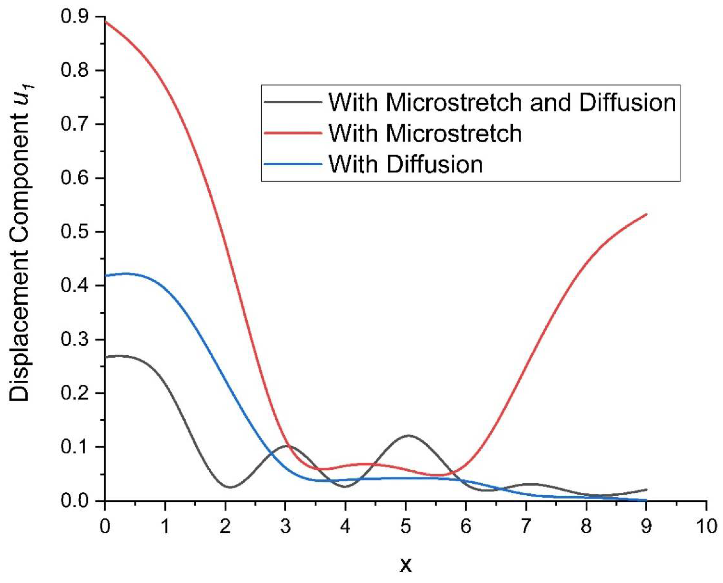
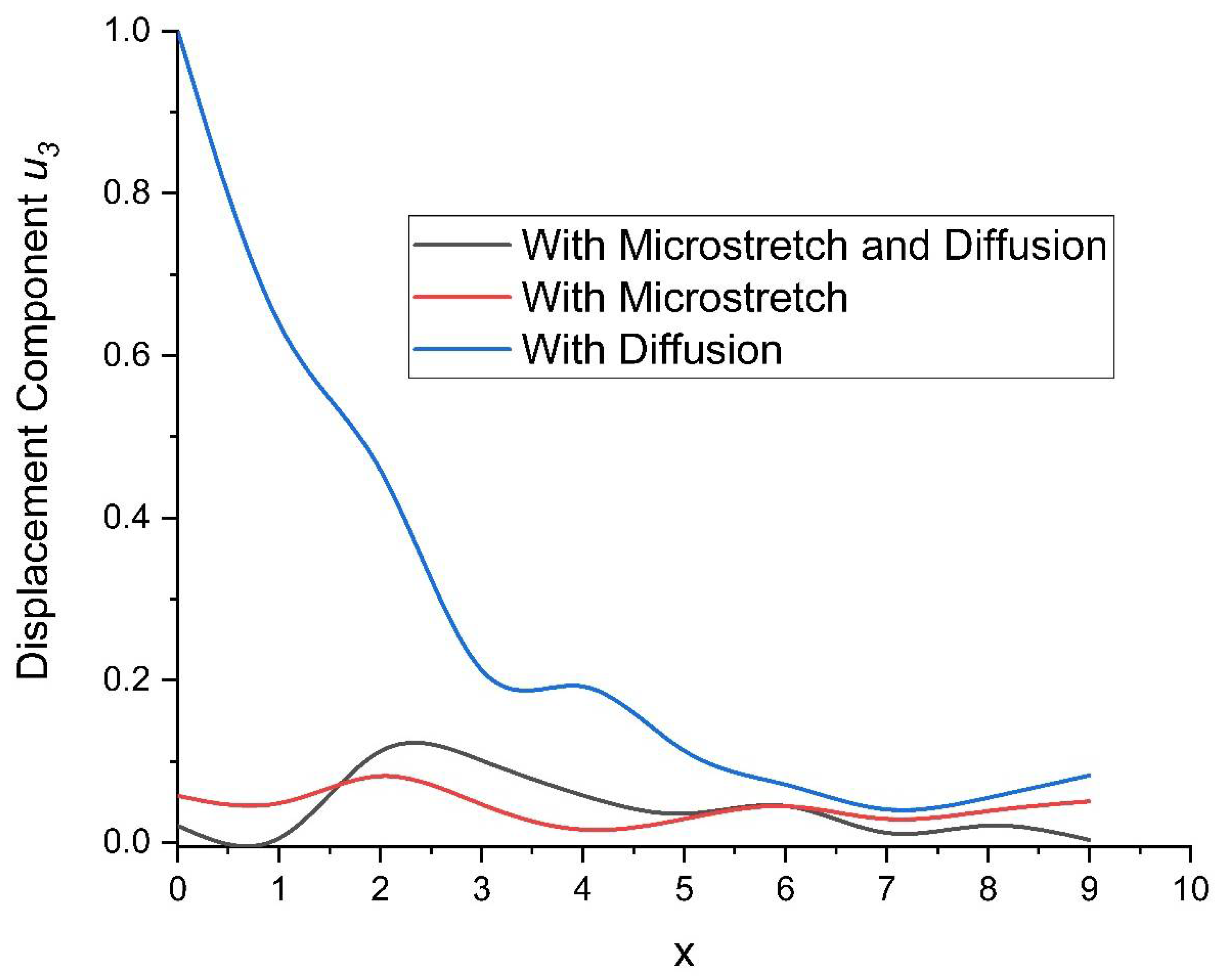
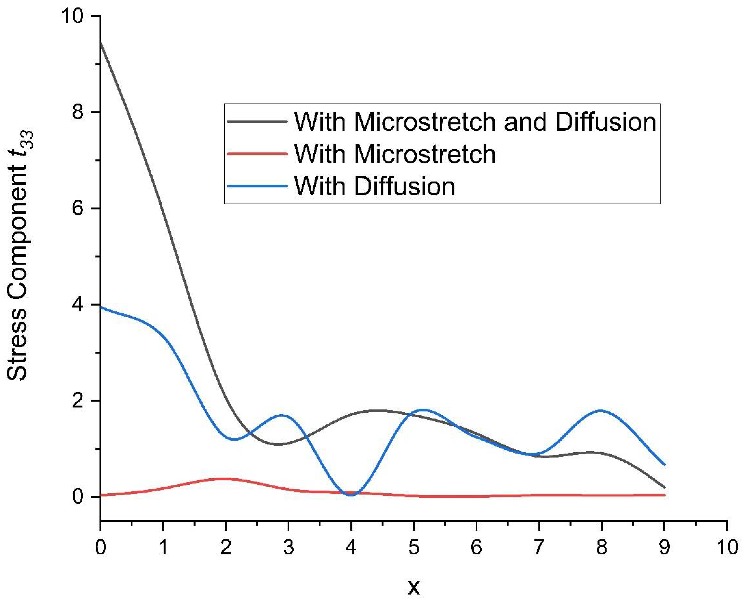
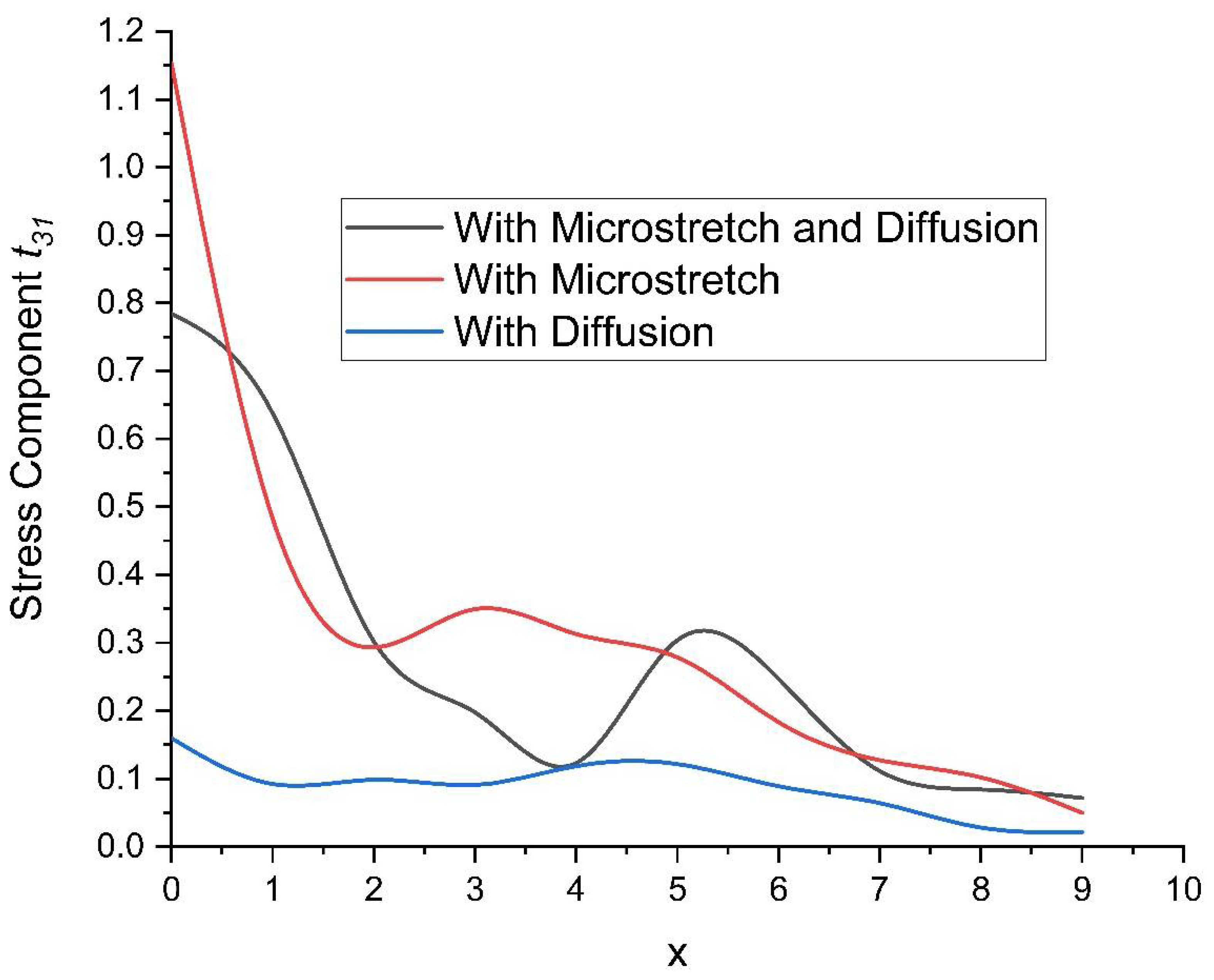
8. Numerical Results and Discussion

To demonstrate our theoretical results and the effect of diffusion and micro-stretching, physical data for magnesium material wad chosen from Eringen [40] as follows:

$$\lambda =9.4\times {10}^{10}N{m}^{-2},\mathrm{\mu }=4.0\times {10}^{10}N{m}^{-2}, K=1.0\times {10}^{10}N{m}^{-2}, \rho =1.74\times {10}^{3}Kg{m}^{-3}, \gamma =0.779\times {10}^{-9}N, j=0.2\times {10}^{-19}{m}^2, C\mathrm{*}=1.04\times {10}^{3}JK{g}^{-1}{K}^{-1}, K\mathrm{*}=1.7\times {10}^{6}J{m}^{-1}{s}^{-1}{K}^{-1}, {\mathsf{\alpha }}_{\mathrm{t}1}=2.33\times {10}^{-5}{K}^{-1}, {\mathsf{\alpha }}_{\mathrm{t}2}=2.48\times {10}^{-5}{K}^{-1}, {\mathsf{\alpha }}_{\mathrm{c}1}=2.65\times {10}^{-4}{m}^{3}K{g}^{-1}, {\mathsf{\alpha }}_{\mathrm{c}2}=2.83\times {10}^{-4}{m}^{3}K{g}^{-1}, T_0=0.298\times {10}^{3}K, a=2.9\times {10}^4{m}^2{s}^{-2}{K}^{-1}, b=32\times {10}^{5}K{g}^{-1}{m}^5{s}^{-2}, D=0.85\times {10}^{-8}Kg{m}^{-3}s, {\tau }_0=0.02s,{\tau }_1=0.01s,{\tau }^0=0.03s,{\tau }^1=0.04s, j_0=0.19\times {10}^{-19}{m}^2,{\alpha }_0=0.779\times {10}^{-9}N,b_0=0.5\times {10}^{-9}N,{\lambda }_0=0.5\times {10}^{10}N{m}^{-2},{\mathrm{a}\mathrm{n}\mathrm{d} \lambda }_1=0.5\times {10}^{10}N{m}^{-2}.$$

In Figure 1, Figure 2, Figure 3, Figure 4, Figure 5, Figure 6, Figure 7 and Figure 8,

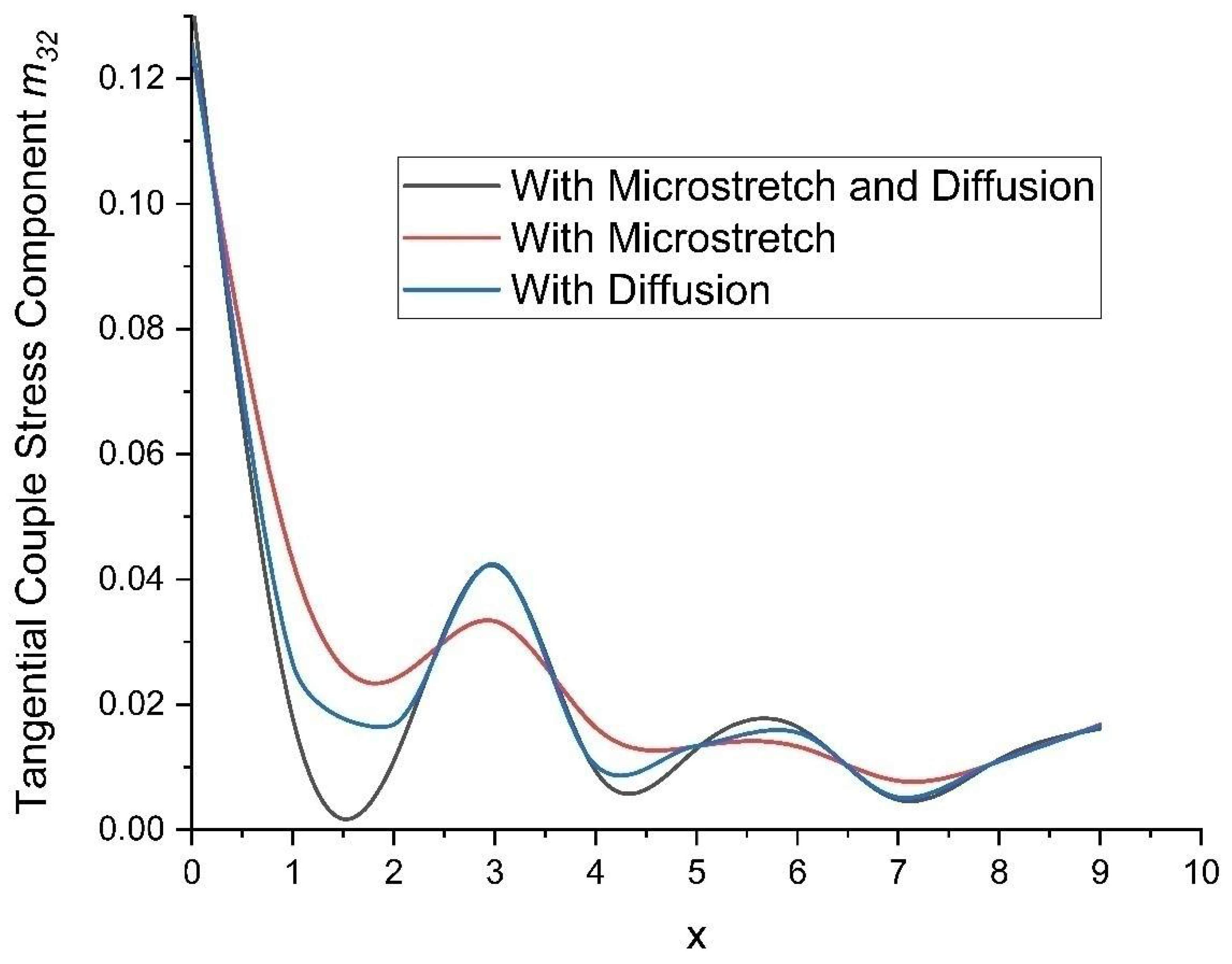
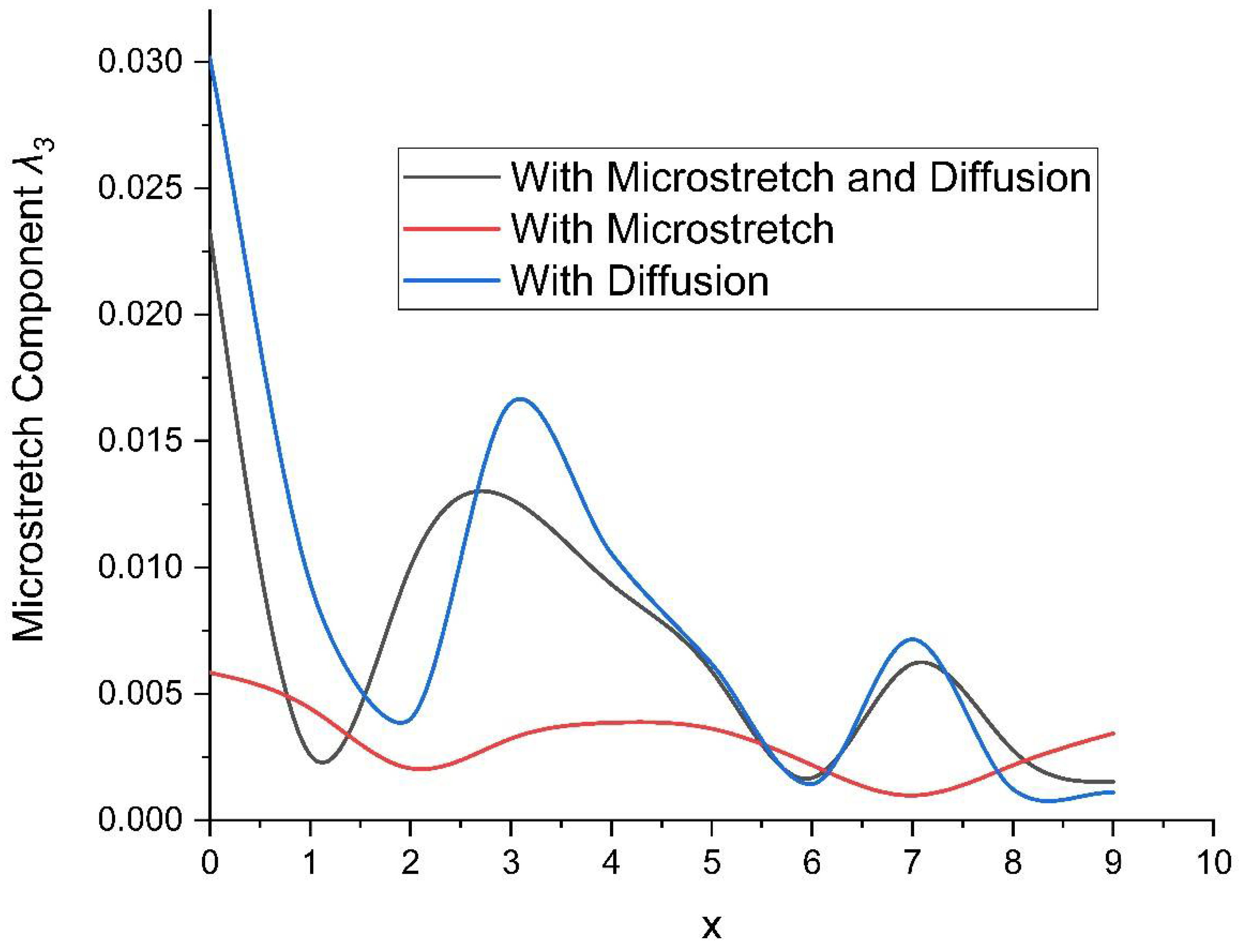
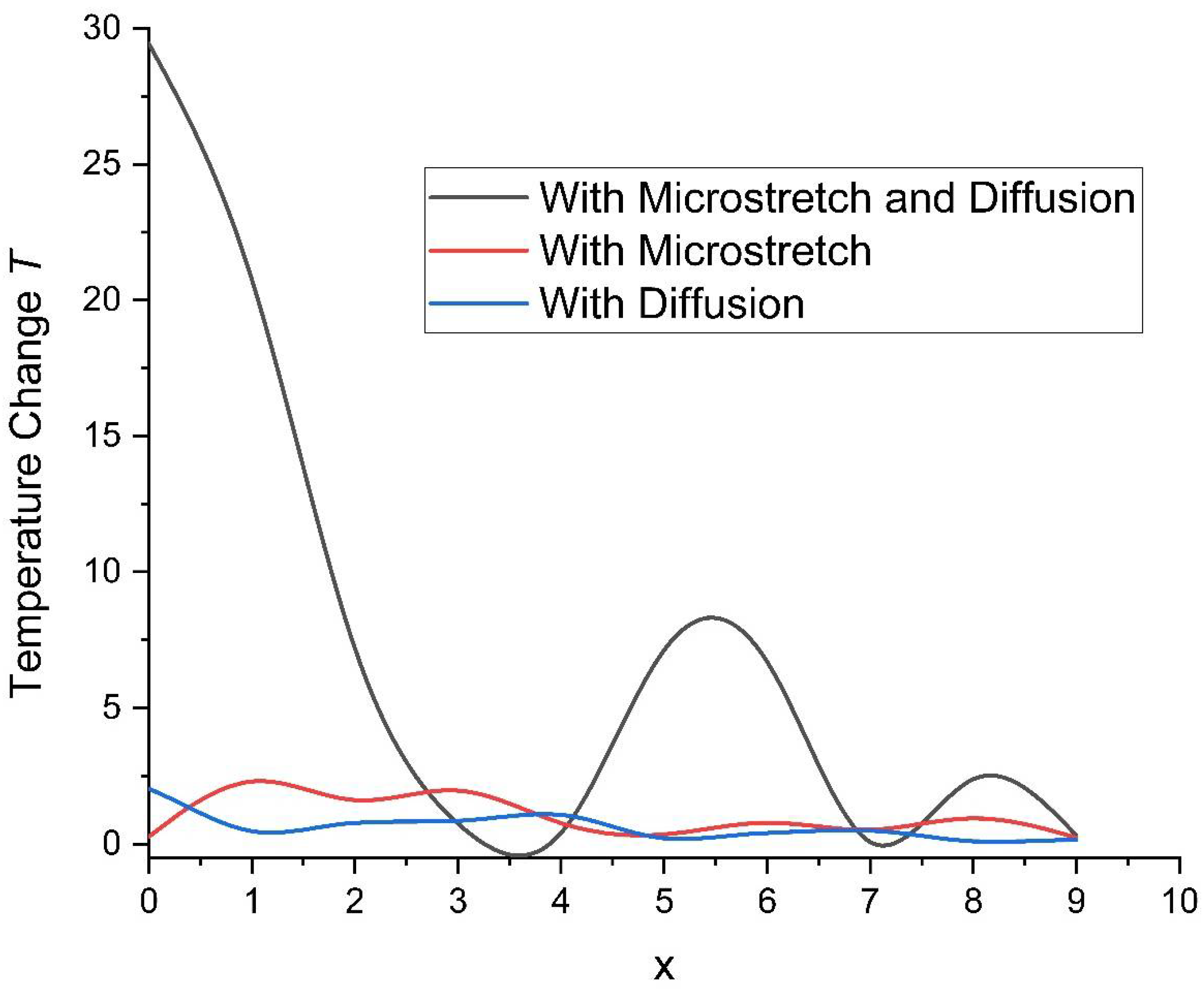
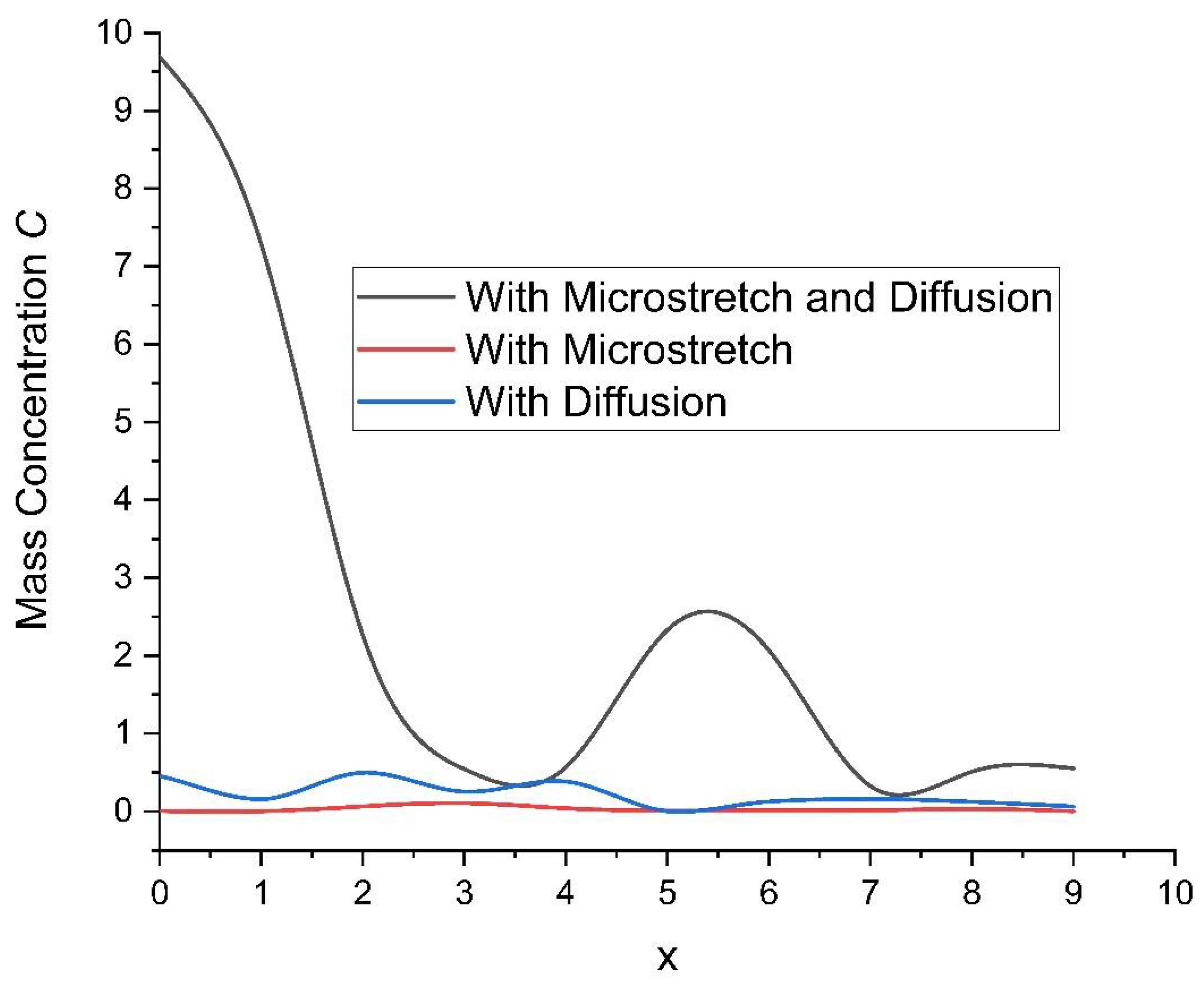
• The black line represents the variations with microstretch and diffusion.
• The red line represents the variations with microstretch neglecting diffusion.
• The blue line represents the variations with diffusion neglecting microstretch.

Figure 1 shows the variation in the displacement component $u_1$ with respect to distance x from the applied source with and without micro-stretching and mass diffusion. It was found that the displacement component $u_1$ decreases as the distance from the applied source increases. In the case of microstretch elastic solids with microstretch and diffusion, the variation of $u_1$ was less pronounced. This means that the displacement of particles or elements in the material is relatively uniform, indicating a higher level of homogeneity. On the other hand, in generalized thermoelastic microstretch half spaces without diffusion, the variation in $u_1$ was at its maximum. This implies that the displacement can vary significantly within the material, showing a lower level of uniformity. Understanding these variations in displacement is crucial for analyzing the behavior of different materials under various conditions and for designing efficient structures and systems.

Figure 2 demonstrates the variation in the displacement component $u_3$ with respect to distance x from the applied source with and without micro-stretching and mass diffusion. The displacement component $u_{3 }$ decreases as the distance from the applied source increases in microstretch elastic solids with microstretch and diffusion. On the other hand, the variation in the displacement component $u_3$ is at its maximum in generalized thermoelastic half spaces without microstretch. This suggests that the behavior of $u_3$ is influenced by the material properties and conditions present. Further exploration and analyses are required to understand the underlying mechanisms and implications of these findings. Figure 3 and Figure 4 exhibit the variation in the stress components $t_{33} \mathrm{a}\mathrm{n}\mathrm{d}{ t}_{31}$ with respect to distance x from the applied source with and without micro-stretching and mass diffusion. The study of stress components in microstretch elastic solids reveals a noteworthy relationship between the distribution of these components and the distance from an applied source. As observed, both $t_{33} \mathrm{a}\mathrm{n}\mathrm{d}{ t}_{31}$ experience a reduction in their values as they move further away from this source. This fascinating behavior accentuates the crucial roles played by the microstretch and diffusion mechanisms in influencing the variation of the stress component $t_{33}$. In addition, the analysis of ${ t}_{31}$ demonstrated that its maximum fluctuation occurs in a generalized thermoelastic half space without microstretch involvement.

Figure 5 exhibits the variation in the tangential couple stress component $m_{32}$ with respect to distance x from the applied source with and without micro-stretching and mass diffusion. It was found that the stress components $t_{33} \mathrm{a}\mathrm{n}\mathrm{d} t_{31}$ decrease as the distance from the applied source increases and exhibits an oscillatory pattern. These results indicate that variation in the tangential couple stress component $m_{32}$arises more under microstretch elastic solids with microstretch and diffusion, and variation in the tangential couple stress component $m_{32}$ occurs less under generalized thermoelastic half spaces without microstretch.

Figure 6 exhibits the variations in the microstretch component with respect to distance x from the applied source with and without micro-stretching and mass diffusion. It was found that the microstretch component decreases as the distance from the applied source increases and exhibits an oscillatory pattern. These results indicate that variation in the microstretch component arises more under microstretch elastic solids with diffusion, and that variation in the microstretch component occurs less under generalized thermoelastic half spaces without microstretch.

Figure 7 and Figure 8 exhibit the variations in temperature change, T, and mass concentration, C, respectively, with respect to distance x from the applied source with and without micro-stretching and mass diffusion. It was found that the temperature change, T, and mass concentration, $C,$ decrease as the distance from the applied source increases and exhibits an oscillatory pattern. These results indicate that variations in temperature change, T, and mass concentration, $C,$ arise more in microstretch elastic solids with microstretch and diffusion, and that variations in temperature change, T, and mass concentration, $C,$ occur less in generalized thermoelastic half spaces without microstretch.

9. Conclusions

The present research provides a complete investigation of mass diffusion and microstretch impact on the thermoelastic disturbances in a homogeneous isotropic microstretch thermoelastic solid. In this framework, the components of displacement, stresses, temperature change, and microstretch as well as couple stress components have been distinguished with and without microstretch and diffusion.

• To estimate the nature of the components of displacement, stresses, temperature change, and microstretch as well as couple stress in the physical domain, an efficient approximate numerical inverse Laplace and Fourier transform technique and Romberg’s integration technique were adopted.
• A comprehensive graphical representation has been provided for a range of variables, detailing the precise effects of mass diffusion and microstretch on thermoelastic deformation through meticulous analysis.
• In the thermo-microstretch theory, the combined effect of microstretch and diffusion is the dominating factor over a single parameter, i.e., microstretch or diffusion.
• It was observed that stress components increase in the microstretch elastic solid with the combined effect of microstretch and diffusion.
• Theoretical analysis and computational findings have substantiated that the impact of mass diffusion and microstretch can amplify the perturbations in the thermoelastic domain.
• The outcome of this problem holds significant value in the realm of two-dimensional dynamic responses, particularly with diverse sources of thermo-diffusion. This phenomenon has numerous applications in both geophysical and industrial domains. The exploration of thermoelasticity is instrumental in enhancing the efficacy of oil extraction processes.

References

1. Eringen, A.C.; Suhubi, E.S. Nonlinear Theory of Simple Micro-Elastic Solids—I. Int. J. Eng. Sci. 1964, 2, 189–203. [Google Scholar] [CrossRef]
2. Suhubl, E.S.; Eringen, A.C. Nonlinear Theory of Micro-Elastic Solids—II. Int. J. Eng. Sci. 1964, 2, 389–404. [Google Scholar] [CrossRef]
3. Eringen, A.C. A Unified Theory of Thermomechanical Materials. Int. J. Eng. Sci. 1966, 4, 179–202. [Google Scholar] [CrossRef]
4. Eringen, A.C. Linear Theory of Micropolar Elasticity. J. Math. Mech. 1966, 15, 909–923. [Google Scholar]
5. Eringen, A.C. Theory of Thermo-Microstretch Elastic Solids. Int. J. Eng. Sci. 1990, 28, 1291–1301. [Google Scholar] [CrossRef]
6. Nowacki, W. Dynamic Problems of Diffusion in Solids. Eng. Fract. Mech. 1976, 8, 261–266. [Google Scholar] [CrossRef]
7. Chandrasekharaiah, D.S. Heat-Flux Dependent Micropolar Thermoelasticity. Int. J. Eng. Sci. 1986, 24, 1389–1395. [Google Scholar] [CrossRef]
8. Eringen, A.C. Microcontinuum Field Theories; Springer: New York, NY, USA, 1999; ISBN 978-1-4612-6815-4. [Google Scholar]
9. Singh, B.; Kumar, R. Wave Propagation in a Generalized Thermo-Microstretch Elastic Solid. Int. J. Eng. Sci. 1998, 36, 891–912. [Google Scholar] [CrossRef]
10. Kumar, R.; Partap, G. Analysis of Free Vibrations for Rayleigh—Lamb Waves in a Microstretch Thermoelastic Plate with Two Relaxation Times. J. Eng. Phys. Thermophys. 2009, 82, 35–46. [Google Scholar] [CrossRef]
11. Kumar, R.; Kansal, T. Fundamental Solution in the Theory of Thermomicrostretch Elastic Diffusive Solids. ISRN Appl. Math. 2011, 2011, 764632. [Google Scholar] [CrossRef]
12. Boschi, E.; Ieşan, D. A Generalized Theory of Linear Micropolar Thermoelasticity. Meccanica 1973, 8, 154–157. [Google Scholar] [CrossRef]
13. Mindlin, R.D. Equations of High Frequency Vibrations of Thermopiezoelectric Crystal Plates. Int. J. Solids Struct. 1974, 10, 625–637. [Google Scholar] [CrossRef]
14. Ciarletta, M. A Theory of Micropolar Thermoelasticity without Energy Dissipation. J. Therm. Stress. 1999, 22, 581–594. [Google Scholar] [CrossRef]
15. Aouadi, M. The Coupled Theory of Micropolar Thermoelastic Diffusion. Acta Mech. 2009, 208, 181–203. [Google Scholar] [CrossRef]
16. Aouadi, M. Theory of Generalized Micropolar Thermoelastic Diffusion Under Lord–Shulman Model. J. Therm. Stress. 2009, 32, 923–942. [Google Scholar] [CrossRef]
17. Aouadi, M. Aspects of Uniqueness in Micropolar Piezoelectric Bodies. Math. Mech. Solids 2008, 13, 499–512. [Google Scholar] [CrossRef]
18. El-Karamany, A.S.; Ezzat, M.A. Uniqueness and Reciprocal Theorems in Linear Micropolar Electro-Magnetic Thermoelasticity with Two Relaxation Times. Mech. Time-Depend. Mater. 2009, 13, 93–115. [Google Scholar] [CrossRef]
19. Marin, M.; Baleanu, D. On mixed problem in thermos-elasticity of type III for Cosserat media. J. Taibah Univ. Sci. 2022, 16, 1264–1274. [Google Scholar] [CrossRef]
20. Groza, G.; Khan, S.A.; Pop, N. Approximate solutions of boundary value problems for ODEs using Newton interpolating series. Carpathian J. Math. 2009, 25, 73–81. [Google Scholar]
21. Modrea, A.; Vlase, S.; Calin, M.R.; Peterlicean, A. The influence of dimensional and structural shifts of the elastic constant values in cylinder fiber composites, J. Optoelectron. Adv. Mater. 2013, 15, 278–283. [Google Scholar]
22. Abo-Dahab, S.M.; Abouelregal, A.E.; Marin, M. Generalized Thermoelastic Functionally Graded on a Thin Slim Strip Non-Gaussian Laser Beam. Symmetry 2020, 12, 1094. [Google Scholar] [CrossRef]
23. Vlase, S.; Teodorescu-Drăghicescu, H.; Calin, M.R.; Scutaru, M.L. Advanced Polylite composite laminate material behavior to tensile stress on weft direction. J. Optoelectron. Adv. Mater. 2012, 14, 658–663. [Google Scholar]
24. Abbas, I.; Hobiny, A.; Marin, M. Photo-thermal interactions in a semi-conductor material with cylindrical cavities and variable thermal conductivity. J. Taibah Univ. Sci. 2020, 14, 1369–1376. [Google Scholar] [CrossRef]
25. Malik, S.; Gupta, D.; Kumar, K.; Sharma, R.K.; Jain, P. Reflection and Transmission of Plane Waves in Nonlocal Generalized Thermoelastic Solid with Diffusion. Mech. Solids 2023, 58, 161–188. [Google Scholar] [CrossRef]
26. Trivedi, N.; Das, S.; Craciun, E.-M. The Mathematical Study of an Edge Crack in Two Different Specified Models under Time-Harmonic Wave Disturbance. Mech. Compos. Mater. 2022, 58, 1–14. [Google Scholar] [CrossRef]
27. Marin, M. On the minimum principle for dipolar materials with stretch. Nonlinear Anal. Real World Appl. 2009, 10, 1572–1578. [Google Scholar] [CrossRef]
28. Gupta, S.; Das, S.; Dutta, R.; Verma, A.K. Higher-Order Fractional and Memory Response in Nonlocal Double Poro-Magneto-Thermoelastic Medium with Temperature-Dependent Properties Excited by Laser Pulse. J. Ocean Eng. Sci. 2022. [Google Scholar] [CrossRef]
29. Zhu, Z.Y.; Liu, Y.L.; Gou, G.Q.; Gao, W.; Chen, J. Effect of Heat Input on Interfacial Characterization of the Butter Joint of Hot-Rolling CP-Ti/Q235 Bimetallic Sheets by Laser + CMT. Sci. Rep. 2021, 11, 10020. [Google Scholar] [CrossRef]
30. Pop, N. A Finite Element Solution for a Three-dimensional Quasistatic frictional Contact Problem. Rev. Roum. Des Sci. Tech. Ser. Mec. Appliq. 1997, 42, 209–218. [Google Scholar]
31. Chen, W.; Hou, H.; Zhang, Y.; Liu, W.; Zhao, Y. Thermal and Solute Diffusion in α-Mg Dendrite Growth of Mg-5wt.%Zn Alloy. J. Mater. Res. Technol. 2023, 24, 8401–8413. [Google Scholar] [CrossRef]
32. Kaur, I.; Singh, K. Rayleigh Wave Propagation in Transversely Isotropic Magneto-Thermoelastic Diffusive Medium with Memory-Dependent Derivatives. Iran. J. Sci. Technol. Trans. Mech. Eng. 2023, 47, 2089–2100. [Google Scholar] [CrossRef]
33. Kaur, I.; Singh, K. Functionally Graded Nonlocal Thermoelastic Nanobeam with Memory-Dependent Derivatives. SN Appl. Sci. 2022, 4, 329. [Google Scholar] [CrossRef]
34. Jafari, M.; Chaleshtari, M.H.B.; Abdolalian, H.; Craciun, E.-M.; Feo, L. Determination of Forces and Moments Per Unit Length in Symmetric Exponential FG Plates with a Quasi-Triangular Hole. Symmetry 2020, 12, 834. [Google Scholar] [CrossRef]
35. Othman, M.I.; Fekry, M.; Marin, M. Plane waves in generalized magneto-thermo-viscoelastic medium with voids under the effect of initial stress and laser pulse heating. Struct. Eng. Mech. 2020, 73, 621–629. [Google Scholar]
36. Marin, M. Some estimates on vibrations in thermoelasticity of dipolar bodies. J. Vib. Control 2020, 16, 33–47. [Google Scholar] [CrossRef]
37. Kuang, W.; Wang, H.; Li, X.; Zhang, J.; Zhou, Q.; Zhao, Y. Application of the Thermodynamic Extremal Principle to Diffusion-Controlled Phase Transformations in Fe-C-X Alloys: Modeling and Applications. Acta Mater. 2018, 159, 16–30. [Google Scholar] [CrossRef]
38. Honig, G.; Hirdes, U. A Method for the Numerical Inversion of Laplace Transforms. J. Comput. Appl. Math. 1984, 10, 113–132. [Google Scholar] [CrossRef]
39. Press, W.H.; Teukolsky, S.A.; Vetterling, W.T.; Flannery, B.P. Numerical Recipes in Fortran; Cambridge University Press: Cambridge, UK, 1980. [Google Scholar]
40. Eringen, A.C. Plane Waves in Nonlocal Micropolar Elasticity. Int. J. Eng. Sci. 1984, 22, 1113–1121. [Google Scholar] [CrossRef]
Figure 1. The variation in the displacement component u 1   with respect to distance x.
Symmetry 15 02095 g001
Figure 2. The variation in the displacement component u 3   with respect to distance x.
Symmetry 15 02095 g002
Figure 3. The variation in the stress component t 33 with respect to distance x.
Symmetry 15 02095 g003
Figure 4. The variation in the stress component t 31 with respect to distance x.
Symmetry 15 02095 g004
Figure 5. The variation in the tangential couple stress component m 32 with respect to distance x.
Symmetry 15 02095 g005
Figure 6. The variations in the microstretch component with respect to distance x.
Symmetry 15 02095 g006
Figure 7. The variations in temperature change, T, with respect to distance x.
Symmetry 15 02095 g007
Figure 8. The variations in mass concentration, C, with respect to distance x.
Symmetry 15 02095 g008
Disclaimer/Publisher’s Note: The statements, opinions and data contained in all publications are solely those of the individual author(s) and contributor(s) and not of MDPI and/or the editor(s). MDPI and/or the editor(s) disclaim responsibility for any injury to people or property resulting from any ideas, methods, instructions or products referred to in the content.