Dimensionless Parameters for Waveform Characterization of Acoustic Emission Signals: Application to Sedimentation and Soil Compression Experiments

Abstract

Acoustic Emission (AE) is a non-destructive evaluation method that uses transient elastic waves produced by the sudden release of mechanical energy in a material or structure. This method generates multiple AE events during testing; therefore, it is important to develop parameters that capture the characteristics of each event (AE hit). The paper introduces new dimensionless parameters to characterize the waveform of AE signals: Earliness, Transitoriness, and Early Transitoriness. The study shows that these parameters provide an accurate description of AE waveforms, in some respects, better than traditional parameters, which makes them suitable for filtering with simple rules or in combination with machine-learning techniques. Two examples of the application of AE hit filtering from sedimentation and soil compression experiments are provided. In the sedimentation test analysis, the proposed parameters were used with K-means clustering to filter AE hits from outside the zone of interest and to calculate the rate of sedimentation. In the compression test of a sand sample under oedometric conditions, a simple filtering rule was applied to discriminate AE hits from unwanted sources and obtain a clear AE energy cumulative curve. In both cases, the dimensionless parameters have shown the capacity to discriminate between different AE sources and paths and the possibility of filtering hits from unwanted sources.

1. Introduction

The transient elastic waves produced by the sudden release of mechanical energy from a source inside a material or structure are known as Acoustic Emission (AE) [1]. These waves can be measured and analyzed to study their sources, leading to a nondestructive evaluation method called the Acoustic Emission Technique (AET). Unlike other acoustic and vibrational non-destructive techniques, such as Ultrasonic Inspection or Modal Analysis, it is a passive method that does not require direct excitation of the material and can monitor processes in real time. This is the drawback and advantage of AET because it cannot be repeated when the process has finished, but it allows the extraction of information about its dynamic characteristics. AET is used in different fields of engineering for different non-destructive evaluations, for instance in health monitoring of concrete [2], masonry [3] and metallic structures [4], soil mechanics [5], and corrosion monitoring [6]. AET is able to monitor many different phenomena, but it is usually difficult to analyze its results and classify different AE mechanisms [7].

Generally, there are two types of AE data: parametric analysis [8,9,10] and signal-based analysis [11]. The first is based on the analysis of AE parameters, which is the set of principal features of an AE discrete wave, which is called an AE hit. The second method is based on the analysis of the waveforms of the recorded AE waves. These approaches have advantages and disadvantages. The signal-based analysis can offer more in-depth information about AE sources, especially when utilizing Moment Tensor Inversion (MTI) [12,13] because of the crack information that it provides. However, it requires more computer capacity for the storage and processing of the recorded data. In addition, it is more dependent on the characteristics of the acquisition equipment and sensors, such as the frequency range. Parameter analysis has been used since the beginning of AET because it requires simpler equipment; therefore, there is much more scientific and technical literature, and its analysis is less dependent on the equipment and sensors used.

The objective of this study is to contribute to the parametric analysis by introducing new dimensionless variables. To the best of the authors’ knowledge, the parameters utilized in parameter analysis are directly characteristics of AE hits or a combination of them but are always dimensional variables. The principal advantage of using dimensionless parameters is that the results are more general and independent of the frequency range of the sensors, which allows for more effective classification of AE signals and their assignment to various source processes.

Machine learning methods are increasingly used in the classification of AE hits according to their sources. Usually, it is difficult to theoretically determine how the AE features are affected by the physical properties of the system under study. Therefore, machine learning methods can help determine how the AE parameters are connected to different AE sources and what the influence of the propagation medium is [14]. The proposed parameters contribute to progress in this field in two ways. First, they increase the variety of available parameters that can be used with machine learning methods. Second, by defining them as relationships between different basic parameters, fewer parameters may be needed for classification, which decreases the complexity and increases the comprehensibility of the process.

2. Parameter Analysis

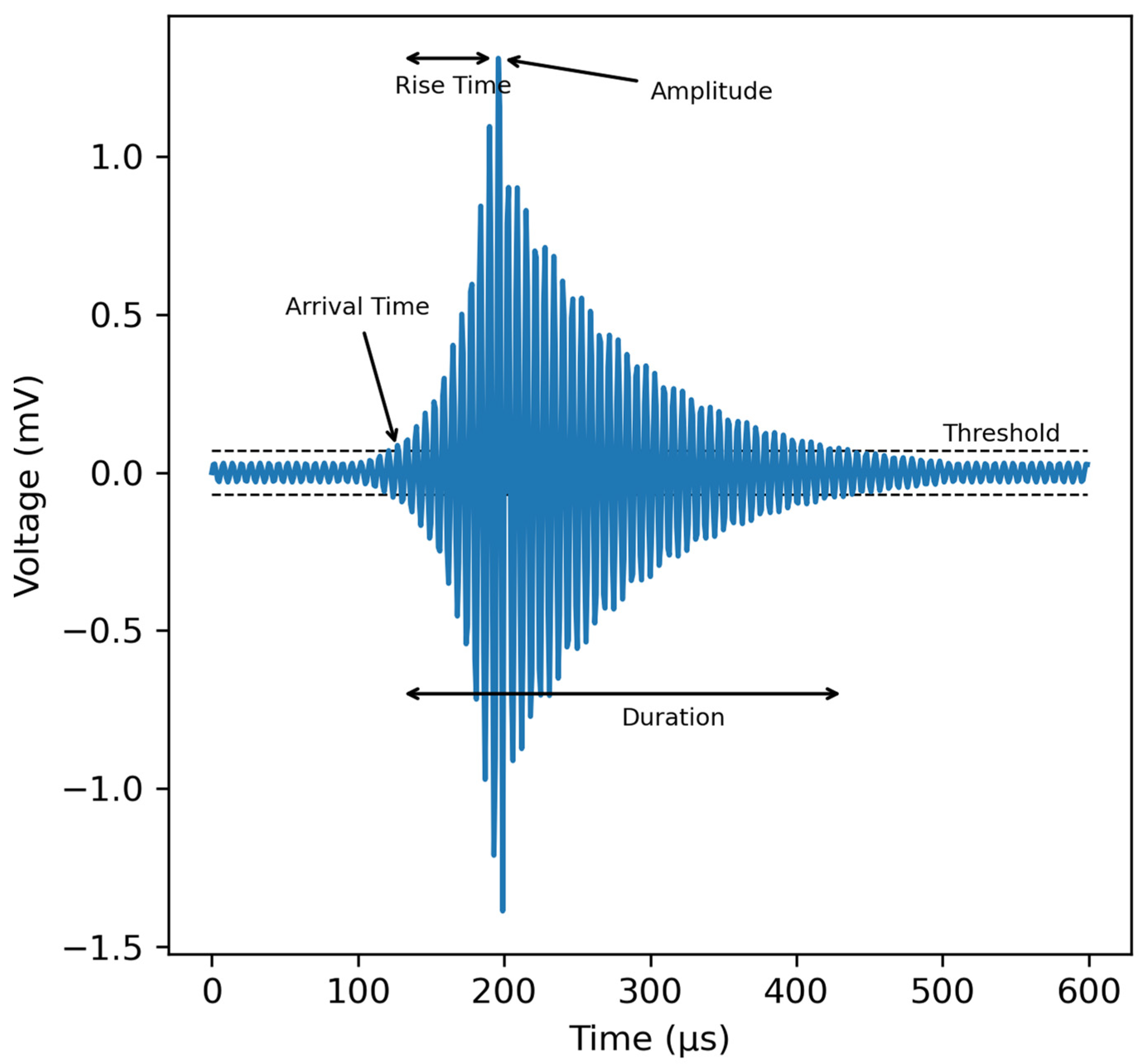
Parameter analysis in AET is based on the extraction and analysis of the hit parameters. An AE hit is a discretized wave detected by a sensor that corresponds to an AE event at the source. An example of an AE hit is shown in Figure 1.

The principal parameters that describe the main characteristics of an AE hit are:

• Amplitude: maximum voltage of the AE hit.
• Arrival time: arrival time of the hit at the sensor. Usually, it is considered the first time that the voltage exceeds a defined threshold.
• Duration: Temporal interval between the first and last time the signal crosses the threshold.
• Rise time: Temporal interval between arrival time and time of maximum voltage.
• Counts: number of times the signal crosses the threshold during its duration.
• Counts to peak: number of times the signal crosses the threshold during the rise time.
• Signal strength: integral of the rectified signal over time.
• Energy: integral of the squared signal over time.

These parameters provide information on the principal physical characteristics of AE hits, and much effort has been made to relate them to their sources. For example, the statistical distribution of hit amplitudes was used to identify cracks in rocks and concrete by applying the “b-value” method [15,16]; the cumulative counts and AE energy rates have been related to different damage stages on rock specimens under different test conditions [17,18]; the amplitude values have been related to the lubricant composition in the monitoring of wire drawing process [19]; and the cumulative AE energy is commonly used to evaluate fatigue damage in concrete beams [20].

The other derived parameters are obtained from these fundamental parameters. They are used to focus on different aspects of AE hits that are not clearly distinguished in fundamental parameters. Because of the large number of AE hits that can be obtained during a test, there is a need for parameters that collect information from AE hits related to the sources, so that they can be analyzed using statistical or machine learning methods.

Some of these derived AE parameters are:

RA value: ratio between the Rise time and the amplitude [21]:

$$\mathrm{R}\mathrm{A}\mathrm{v}\mathrm{a}\mathrm{l}\mathrm{u}\mathrm{e}=\frac{\mathrm{R}\mathrm{i}\mathrm{s}\mathrm{e}\mathrm{t}\mathrm{i}\mathrm{m}\mathrm{e}}{\mathrm{A}\mathrm{m}\mathrm{p}\mathrm{l}\mathrm{i}\mathrm{t}\mathrm{u}\mathrm{d}\mathrm{e}}$$

It quantifies the shape of the first part of the waveform, which is related to the different excitations of the wave modes by the different crack types. Tensile cracks create longitudinal waves because of the transient volumetric change that is produced by these cracks, whereas shear cracks mostly produce shear waves, which are slower than longitudinal ones. Therefore, the maximum amplitude arrives later in the shear waves than in the longitudinal waves, resulting in longer Rise times. As the Rise time also depends on the Amplitude, the RA value is used to quantify the duration of the Rise time according to its Amplitude.

Average Frequency (AF): is the ratio between the counts and the duration [22]:

$$\mathrm{A}\mathrm{F}=\frac{\mathrm{C}\mathrm{o}\mathrm{u}\mathrm{n}\mathrm{t}\mathrm{s}}{\mathrm{D}\mathrm{u}\mathrm{r}\mathrm{a}\mathrm{t}\mathrm{i}\mathrm{o}\mathrm{n}}$$

It is a measure of the overall frequency of the signal and is used together with the RA value to classify the cracks [23] and determine its mode, leading to the RA-AF analysis. It has been shown that tensile cracks produce higher frequency signals than shear cracks [21].

3. Dimensionless Parameters

There are differences between the waveform of the elastic wave when it originates from the source and its record after its arrival at the sensor [24]. First, the propagation in the medium attenuates and disperses the wave until it arrives at the sensor. After its arrival, the physical characteristics of the sensor determine its transfer function and how it is measured. Finally, the electronic instrumentation of the acquisition equipment (signal amplification and analog filters) also influences the final signal record.

The dependence of the waveform on all these factors indicates that the AE parameters shown in the previous section depend not only on the source but also on the material properties of the medium, geometrical configuration of the medium, source and sensors, and electronic equipment. This limits the applicability of parameter analyses, particularly when different sensors and electronic equipment are used.

This paper proposes the use of dimensionless parameters to overcome this issue and obtain more general results from AE parameter analysis. Being dimensionless makes them less dependent on the frequency response of the measuring equipment because ratios of similar physical magnitudes are used, such as the ratio of two relevant times of the signal. In addition, dimensionless parameters are designed to reflect the principal features of the waveform shape in a manner that is less dependent on the measurement properties and acquisition settings of the sensors and electronic equipment. Their range of values is between 0 and 1, which allows a comparison between tests with different physical systems and the attribution of the range of values for different sources.

The first dimensionless parameter is the ratio of the rise time of the signal to its duration. It is a measure of how early the peak amplitude occurs relative to the whole duration of the signal; therefore, this parameter has been called Earliness and earl in abbreviated form:

$$\mathrm{E}\mathrm{a}\mathrm{r}\mathrm{l}\mathrm{i}\mathrm{n}\mathrm{e}\mathrm{s}\mathrm{s}=\mathrm{e}\mathrm{a}\mathrm{r}\mathrm{l}=\frac{\mathrm{R}\mathrm{i}\mathrm{s}\mathrm{e}\mathrm{T}\mathrm{i}\mathrm{m}\mathrm{e}}{\mathrm{D}\mathrm{u}\mathrm{r}\mathrm{a}\mathrm{t}\mathrm{i}\mathrm{o}\mathrm{n}}$$

A low value of this parameter means that the peak amplitude occurs very early with respect to the duration, whereas a value near one means that the peak amplitude arrives very late. A value of approximately 0.5 implies some kind of symmetry in the waveform, with the maximum of the signal in its center and the same rise and decay time.

The second dimensionless parameter is the ratio between the signal strength and peak amplitude multiplied by the duration:

$$\mathrm{T}\mathrm{r}\mathrm{a}\mathrm{n}\mathrm{s}\mathrm{i}\mathrm{t}\mathrm{o}\mathrm{r}\mathrm{i}\mathrm{n}\mathrm{e}\mathrm{s}\mathrm{s}=\mathrm{T}\mathrm{r}=\frac{\mathrm{S}\mathrm{i}\mathrm{g}\mathrm{n}\mathrm{a}\mathrm{l}\mathrm{S}\mathrm{t}\mathrm{r}\mathrm{e}\mathrm{n}\mathrm{g}\mathrm{t}\mathrm{h}}{\mathrm{P}\mathrm{e}\mathrm{a}\mathrm{k}\mathrm{A}\mathrm{m}\mathrm{p}\mathrm{l}\mathrm{i}\mathrm{t}\mathrm{u}\mathrm{d}\mathrm{e}\ast \mathrm{D}\mathrm{u}\mathrm{r}\mathrm{a}\mathrm{t}\mathrm{i}\mathrm{o}\mathrm{n}}$$

It is called Transitoriness because it is a measure of how transient the hit is, but it requires an explanation to be understood. A typical transient hit is shown in Figure 1, which is strongly asymmetric because there is a rapid increase in the signal until it reaches its maximum, followed by a slow exponential decay. Another type of hit is a stationary hit, in which its amplitude changes little with time, and its waveform is more symmetric. A representation of this type of hit is shown in Figure 2.

This kind of hit is produced by a long-lasting source, whereas a transient hit is produced by a fast and almost instant source. Depending on the application, we would analyze stationary or transient hits. For example, different wear phenomena are associated with transient or stationary hits [25]. Using the Transitoriness, it can be possible to discriminate between transient and stationary hits.

The relationship between the definition of Transitoriness and its capacity to discriminate between transient and stationary hits exists because, for fixed peak amplitude and duration, the signal strength of a stationary hit is higher than that of a transient hit. This is because the amplitude of a transient hit decays faster than that of a stationary hit, and most amplitude values are lower. Therefore, the area under the signal is larger for a stationary hit than for a transient hit with the same peak amplitude and duration.

However, signal strength alone cannot be used to discriminate between stationary and transient hits, because hits usually have different peak amplitudes and durations. So, it is necessary to normalize it in some way. To achieve this, the signal strength of a constant hit with the same peak amplitude and duration as that of the hit can be employed. The signal strength of a hit with constant amplitude (see Figure 3) is the maximum possible for a specific peak amplitude and duration. Therefore, the ratio of the signal strength of any hit to that of a constant is a number between zero and one. The more stationary a hit is, the higher its signal strength and the closer its Transitoriness is to one (i.e., it is more similar to a constant hit). In contrast, the signal strength of a transient hit is lower, and its Transitoriness is closer to zero. Figure 3 illustrates a comparison between the signal strengths of a transient, stationary, and constant hit, which aids in better understanding this explanation.

A low value of Transitoriness means that the hit is very transient, whereas a value near one indicates that the signal amplitude is almost constant, so the hit is very continuous.

The last dimensionless parameter is the Early Transitoriness (eTr). It is based on Transitoriness but uses only the signal strength of the signal until the maximum and the rise time instead of the duration:

$$\mathrm{E}\mathrm{a}\mathrm{r}\mathrm{l}\mathrm{y}\mathrm{T}\mathrm{r}\mathrm{a}\mathrm{n}\mathrm{s}\mathrm{i}\mathrm{t}\mathrm{o}\mathrm{r}\mathrm{i}\mathrm{n}\mathrm{e}\mathrm{s}\mathrm{s}=\mathrm{e}\mathrm{T}\mathrm{r}=\frac{\mathrm{S}\mathrm{i}\mathrm{g}\mathrm{n}\mathrm{a}\mathrm{l}\mathrm{S}\mathrm{t}\mathrm{r}\mathrm{e}\mathrm{n}\mathrm{g}\mathrm{t}\mathrm{h}\mathrm{u}\mathrm{n}\mathrm{t}\mathrm{i}\mathrm{l}\mathrm{P}\mathrm{e}\mathrm{a}\mathrm{k}\mathrm{A}\mathrm{m}\mathrm{p}\mathrm{l}\mathrm{i}\mathrm{t}\mathrm{u}\mathrm{d}\mathrm{e}}{\mathrm{P}\mathrm{e}\mathrm{a}\mathrm{k}\mathrm{A}\mathrm{m}\mathrm{p}\mathrm{l}\mathrm{i}\mathrm{t}\mathrm{u}\mathrm{d}\mathrm{e}\ast \mathrm{R}\mathrm{i}\mathrm{s}\mathrm{e}\mathrm{T}\mathrm{i}\mathrm{m}\mathrm{e}}$$

Thus, it is the Transitoriness as if the hit would finish at the rise time. Therefore, it is a measure of how transient or continuous the first part of the signal is.

The reason for using only the first part of the hit in the calculation of eTr is to obtain a dimensionless parameter with a similar role to RA, that is, to characterize the part of the signal before the peak amplitude. Therefore, it is possible to check if the signal has a much lower amplitude than the peak amplitude until just before the rise time or if the amplitude before the rise time has similar values to the peak amplitude. As an example, the transient and continuous signals shown in Figure 3 have the same eTr because their amplitude evolutions before the peak amplitude are the same; thus, eTr can be used in conjunction with Tr to observe the similarities and differences in the waveform. Concerning its relationship with RA, a hit with a high RA value typically has a high value of eTr; therefore, eTr can be used as a dimensionless substitute for RA.

Four examples of typical AE signals are shown in Figure 4, and the values of their parameters (dimensionless, typical, and derived) are listed in

Table 1. Values of several parameters of signals from Figure 4.

Parameters	Signal A	Signal B	Signal C	Signal D
Earliness	0.0069	0.0722	0.1868	0.1468
Transitoriness	0.0497	0.0764	0.0508	0.2046
Early Transitoriness	0.295	0.251	0.097	0.21
Peak amplitude	9.88	6.46	38	0.37
Duration (ms)	57	39.8	19.5	16.1
Rise time (ms)	0.39	2.87	3.64	2.37
Signal strength (µVs)	28	19.6	37.7	1.21
AE energy (10−8 V2s)	5.66	3.56	44	0.014
RA value	0.04	0.444	0.096	6.406
AM	46,700	37,400	39,200	35,900

. The first AE hit (A) is a typical transient hit with a fast increase in amplitude (low rise time) and an exponential decay after the peak amplitude. The fast first rise and subsequent slow decay indicate that the peak amplitude is reached very early with respect to its duration; therefore, its Earliness is very low. The concentration of higher amplitude values in a small zone owing to the decay of the amplitude makes the Transitoriness very low. Concerning Early Transitoriness, the amplitude values were very high at the beginning of the hit (before the peak amplitude). Thus, eTr is relatively high. The second hit (B) is also a typical transient hit, but the peak amplitude occurs later than that of the first hit. This means that its Earliness is an order of magnitude higher than that of hit A, whereas the values of Transitoriness and Early Transitoriness are similar because the other characteristics of the waveform are similar. The third AE hit (C) appears to be composed of several transient waveforms. The peak amplitude was not reached at the beginning of the hit, but approximately when one-fifth of the duration elapsed. Therefore, its Earliness is much higher than those of hits A and B. Because of the transient nature of hit C, its Transitoriness is very low. In this case, Early Transitoriness is low because of the low amplitude values before the peak amplitude. The last AE hit (D) is a typical stationary AE hit, which is reflected in its high Transitoriness. The almost constant amplitude values also produce a high Early Transitoriness. In the case of Earliness, it is similar to hit C because the peak amplitude is reached in a similar part of the waveform.

Notably, the four AE hits have very different values for the amplitude, duration, rise time, and other AE parameters. However, the proposed dimensionless parameters allow the analysis of their waveforms and find similarities and differences in a manner that other AE parameters cannot. The first three AE hits (A, B, and C) are transient and thus have similar Transitoriness values. However, it is difficult to determine it from their amplitude, duration, and signal strength, which are used to calculate Transitoriness. Hits A and B have similar amplitudes, durations, signal strengths, and energies, indicating that they are similar. Despite this, we cannot say anything about the transient nature of the hits from these values. Hit C is also a transient hit, but its basic parameters are very different from those of hits A and B. Hit D is a continuous hit, with a Transitoriness much higher than the other three hits. However, it is difficult to know it from its basic parameters because its duration is shorter than hits A and B and similar to C, its rise time is similar to that of B and C, while its amplitude, energy, and signal strength are much lower than those of the other three. Therefore, it is difficult to establish a rule for the transient nature of a hit based on its basic parameters.

From the derived parameters RA and AM, it is also difficult to analyze the waveforms and detect similarities and differences. Although RA provides information about the initial rise until the peak amplitude, the values in Table 1 do not exhibit a clear pattern. The RA values of hits A and C are similar, yet their initial signals differ. Hit D has a high RA value because of its low peak amplitude, but its initial signal is similar to that of hit B. Early Transitoriness describes the first section of a hit more accurately, with hits A, B, and D sharing similar initial amplitudes and Early Transitoriness values. Conversely, hit C starts with low amplitude values and rises and drops before reaching the peak amplitude, and its Early Transitoriness is significantly lower than that of the other hits. The AM appears to be related to the transient nature of the waveforms, with higher values corresponding to more transient signals (except for hits B and C). However, the differences in AM values do not always correspond to changes in the waveforms because there is a greater difference between the values of hits A and B than between hits B and D.

4. Examples of Application to Experimental Cases

To test the feasibility of the parameters, they have been used to analyze the AE of hits produced in different experimental situations. The main objective was to test them and determine if they were useful for AE analysis. In all cases, a Vallen ANSY-6 system from Vallen Systeme was used to record the AE hits.

4.1. AE Hits from Different Sources in a Metallic Bar

In the first experiment, two AE sensors were placed on top of a metallic bar. The objective was to determine whether the proposed dimensionless parameters exhibited different values for the different types of AE hits. To produce them, a Hsu-Nielsen source and different instruments were applied to the top of the metallic bar to act as AE sources. The AE sources, which are listed in

Table 2. Table of the AE sources applied to the metallic bar.

AE Source	Description
Hsu-Nielsen source	Pencil lead break. It is a standard method to produce highly reproducible transient AE hits.
Punch	The pointed end of the punch is used to hit the metallic bar at a specific point.
File	The tip of a file is used to hit the metallic bar at a specific point.
Soft plastic hammer	A soft plastic hammer is used to hit the metallic bar at a specific point.
Soft rubber hammer	A soft rubber hammer is used to hit the metallic bar at a specific point.

, were chosen to produce different types of hits (stationary, transient, different duration and amplitude, etc.) because of their different hardness and area of impact.

The experiment was performed twice, each time with a different type of AE sensor. The first was VS30-SIC, from Vallen Systeme, with an integrated preamplifier of 46 dB and a frequency band of 25–80 kHz. The second was a VS900-RIC, also from Vallen Systeme, with an integrated preamplifier of 34 dB and a frequency band of 100–900 kHz. The objective was to determine the differences in the values of dimensionless parameters using two types of sensors with very different frequency bands. The values of the dimensionless parameters are shown in Figure 5 (25–80 kHz sensors) and Figure 6 (100–900 kHz sensors).

The AE hits from the Hsu-Nielsen source have very similar values. This is due to the fact that this is a source that produces very reproducible hits, so their values are very similar. Their Earliness and Transitoriness are very low, meaning that they reach their peak amplitudes very early and decay quickly. The Early Transitoriness has more variability, with values around 0.2. These values indicate that the rise to the peak amplitude occurs quickly, with high values of amplitude at the beginning.

The features of AE hits produced by other AE sources can be connected to the physical characteristics of the tools. AE hits from the application of the pointed end of the punch are very similar to the Hsu-Nielse hits: they are transient (very low Transitoriness), with a fast arrival of the peak amplitude (very low Earliness) and with a fast rise of the amplitude until peak amplitude (Early Transitoriness around 0.1–0.2). This is because the application of the pointed end of the punch can be performed in a fast and precise manner, which is similar to the application of the Hsu-Nielsen source.

The file also produces transient hits because it is formed by a metallic hard material; however, the larger contact area has several impacts at the same time, which produces several ultrasound waves that superpose in a single AE hit. Thus, the peak amplitude is reached later, as can be seen from the Earliness. The dispersion of the values was also higher because each time the impact of the file was different, the AE hits also differed.

This dispersion of the values can also be found in the application of both hammers, because each time the area of contact is different. The Earliness and Transitoriness are high, meaning that the hits are more stationary, probably because the large area of the hammers and softer material makes the impact take longer and the impact energy is distributed over a longer period of time.

The values of the dimensionless parameters were very similar when two types of sensors were used, as shown in

Table 3. Mean value and standard deviation (mean ± standard deviation) of the dimensionless parameters. AE hits were measured with 25–80 kHz sensors for the different AE sources.

AE Source	Earliness	Transitoriness	Early Transitoriness
Hsu-Nielsen source	0.02 ± 0.03	0.053 ± 0.009	0.24 ± 0.04
Punch	0.05 ± 0.07	0.05 ± 0.04	0.15 ± 0.06
File	0.11 ± 0.15	0.07 ± 0.06	0.14 ± 0.08
Soft plastic hammer	0.15 ± 0.19	0.16 ± 0.08	0.26 ± 0.07
Soft rubber hammer	0.14 ± 0.13	0.03 ± 0.02	0.07 ± 0.05

and

Table 4. Mean value and standard deviation (mean ± standard deviation) of the dimensionless parameters. AE hits were measured with 100–900 kHz sensors for the different AE sources.

AE Source	Earliness	Transitoriness	Early Transitoriness
Hsu-Nielsen source	0.012 ± 0.013	0.07 ± 0.06	0.18 ± 0.04
Punch	0.04 ± 0.03	0.062 ± 0.017	0.19 ± 0.04
File	0.07 ± 0.08	0.10 ± 0.06	0.18 ± 0.06
Soft plastic hammer	0.07 ± 0.06	0.15 ± 0.05	0.18 ± 0.06
Soft rubber hammer	0.12 ± 0.16	0.13 ± 0.09	0.18 ± 0.08

. This is because they are based on the waveform and not on features that can be affected by the frequency range of the sensors. This means that as long as the waveforms are similar for different frequency ranges, the classifications that are performed with dimensionless parameters can be generally applied independently of the type of sensors that are used. Only the Transitoriness of AE hits from the soft rubber hammer was significantly different between the two types of sensors.

4.2. AE Hits with Different Propagation Paths

In this section, we investigate the changes in the values of the dimensionless parameters of an AE ultrasound when measured at two different positions with very different propagation paths from the source. Two steel plates were placed inside a plastic container. Two AE sensors of VS30-SIC from Vallen Systeme, with an integrated preamplifier of 46 dB and a frequency band of 25–80 kHz, were located in each of the steel plates, as shown in Figure 7. A Hsu-Nielsen source was applied several times in each of the plates, so the AE hits that were produced were recorded by the sensor on the same plate and the sensor on the other plate. This allows us to check the differences between the waveform when it is recorded in the same plate that is produced (with a direct pathway) and when there are changes in the propagation medium (steel-plastic-steel).

Figure 8 shows the values of the dimensionless parameters for the AE signals recorded in the same plate as the source and the other plate. The values of Earliness and Transitoriness are much lower for AE signals recorded by the sensor in the same plate as the source, whereas the values of Early Transitoriness are similar. This means that the changes in the waveform during propagation cause the peak amplitude to occur later, and the changes in amplitude are attenuated, making it more stationary.

4.3. AE Hits from a Sedimentation Process

In this section, the AE technique was used to monitor the evolution of the sedimentation process and obtain relevant information. To do so, the plastic container and two AE sensors over the plates of the previous section were used with the same experimental configuration. The plastic container was partially filled with water, and pyrite particles were dropped on it while the AE sensors were recorded. The sedimentation process was monitored using AE sensors during and after dropping pyrite particles. They recorded the ultrasonic waves produced by the impact of particles on the floor of the plastic container and steel plates. It is assumed that each AE signal recorded by the sensor was produced by the hit of a particle; therefore, by counting the number of AE signals, it is possible to determine the rate of sedimentation of the pyrite particles.

An important experimental parameter that is fundamental for accurate monitoring of the sedimentation process is the area of the floor where the AE sensors can measure the ultrasounds produced by particle hits. The amplitude attenuation on the steel plates was very low; therefore, all hits of the steel plate were recorded by the corresponding AE sensor. However, as we have seen in the previous subsection, it is possible that an AE hit produced in one steel plate was also recorded by the AE sensor in the other steel plate. In addition, it is possible that a particle hitting the plastic floor produces an AE signal in one of the AE sensors on the plates.

To differentiate between the AE signals of hits on the steel plate and outside hits, we can use the information obtained in the previous subsection. We have observed from the Transitoriness and Earliness of the AE signals from sources on the same plate that the sensors have lower values than the AE hits from the other plate. As this is due to the modification of the waveform during the propagation path to the sensor, it is reasonable to assume that AE signals from AE sources on the plastic floor will suffer a similar distortion. Therefore, we have two different groups of AE signals with different Transitoriness and Earliness values: AE signals from the steel plate where the sensor is located, and AE signals from the outside.

To distinguish between the AE signals of hits on the steel plate and outside hits, a partitional clustering technique can be used to obtain the natural groupings in the dataset of Earliness and Transitoriness. Clustering techniques are commonly used in the analysis of AE results to find relationships between AE parameters and AE sources and processes [26,27]. One of the objectives of this article is to increase the availability of characterization parameters for clustering to contribute to the advancement of the field.

One of the simplest and most commonly used partitional clustering methods is the K-means algorithm [28]. This algorithm divides a dataset into a number (K) of different clusters by the minimization of the sum of the squared distance between the elements of the dataset and the centroid of the cluster [29]. So, giving a dataset X, it is divided into K non-overlapping groups G = {g₁, g₂, …, g_K} with gi ≠ Ø, ${\cup }_1^K{g}_i=\mathrm{X};g_i\cap g_i=$ Ø; i, j = 1, …, K and i ≠ j. For each group g_i, an objective function J_i is defined as the sum of the squared distances between each point x_i,h of group g_i (x_i,h ∈ g_i, with h = 1,…, n_i, and n_i the number of elements of g_i) and its centroid (c_i):

$$J_i={\sum }_{h=1}^{n_i}{‖x_{i,h}-c_i‖}^2.$$

(1)

The elements that belong to each group or cluster are determined by the minimization of the function J, defined as the sum of the functions J_i:

$$J={\sum }_{i=1}^K{J}_i.$$

(2)

In our problem, the dataset was composed of a 2-dimensional vector where each element was defined by the Earliness and Transitoriness of each AE signal. The Euclidean distance was considered, and Lloyds’ algorithm was used to minimize the function J.

The distribution and structure of data can influence the performance and results of the clustering technique [30]. Therefore, the appropriate first step in the application of the K-means technique is data normalization [31]. This ensured that all data had a similar scale between 0 and 1. When using dimensionless parameters as datasets, this is unnecessary because they are naturally distributed between 0 and 1.

For clustering using the K-means technique, it is necessary to specify the number K of clusters and their initial centroid, which will be updated during the different iterations of Lloyds’ algorithm. Although there are several methods to deal with the problem of specifying the number of clusters and initial centroids [32], in our case, we have physical information that there are only two clusters (AE signals from the steel plate or outside) and that one has lower values of Earliness and Transitoriness than the other. Therefore, we chose the points (0,0) and (1,1) as initial centroids to ensure that the dataset is separated into two groups of low and high Transitoriness and Earliness values. Random initial centroids were also tested; however, the resulting clusters were similar to those obtained using the chosen initial centroids.

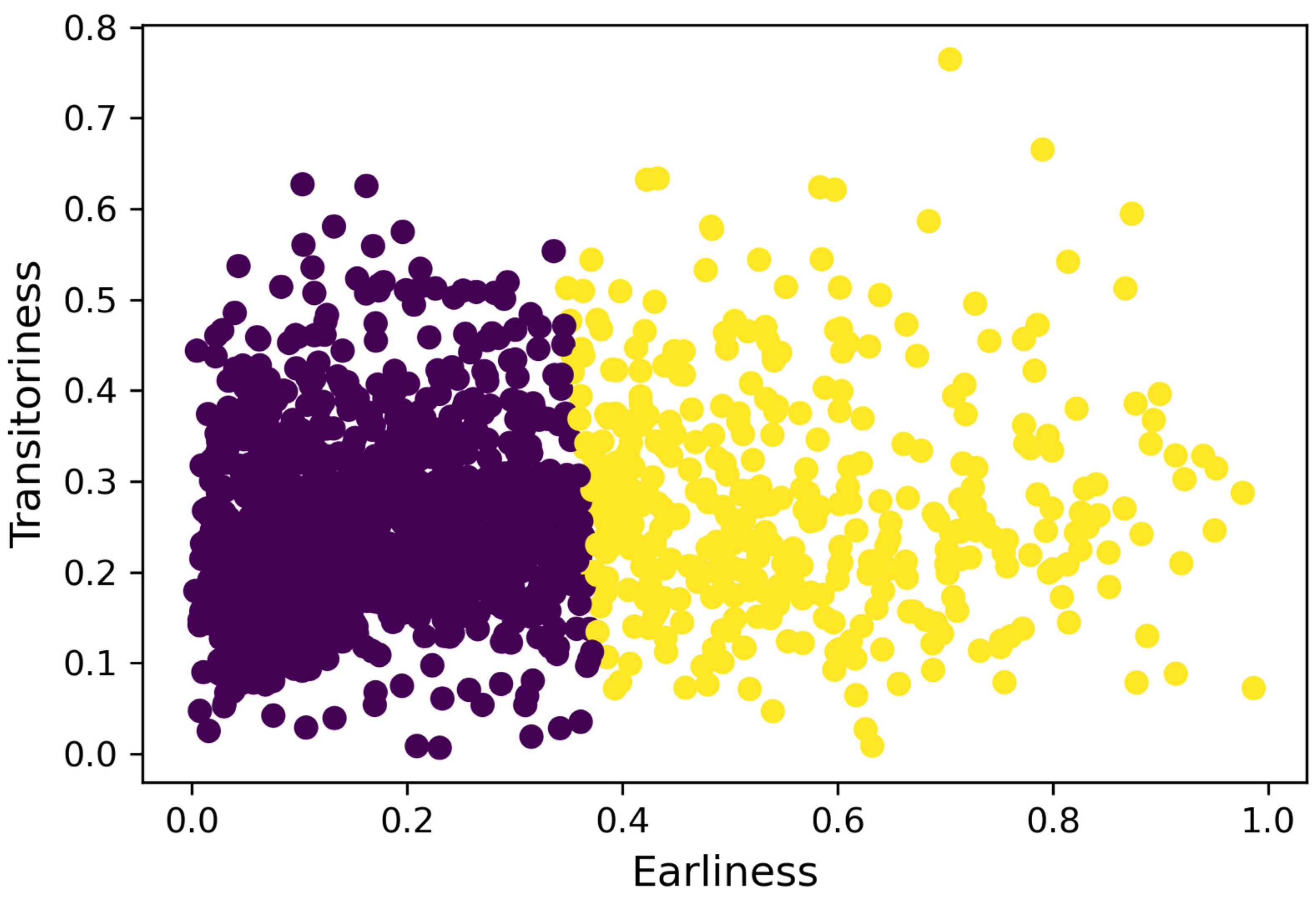
In Figure 9, the distribution of the Earliness and Transitoriness values and their classification into the two groups is shown. It can be observed that the classification is principally based on Earliness, with a small influence of Transitoriness. The first cluster is composed of AE signals with lower values of Earliness; therefore, it is assumed that AE hits from this group are produced on the steel plate where the AE sensor is located, whereas the AE hits from the second cluster are assumed to originate outside the steel plate where the AE sensor is located.

To analyze the sedimentation process, Figure 10 shows the cumulative number of AE hits from the first cluster. Three different phases can be seen in this figure for both sensors according to the different processes that occur at different times of sedimentation. Initially, there was a rapid increase in the curve during the first 30 s, which means that at the beginning, a high number of AE hits were produced. This phase corresponds to the incorporation of pyrite particles into the water, with many of them dropping directly onto the floor. Subsequently, there is a flat zone on the curve, with a duration of 500–600 s, which corresponds to a phase in which the particles remained in suspension in water, with a very low number of particles reaching the floor. In the last phase, there was an increase in the rate of AE hits, which means that the suspended particles have started to sediment. The almost constant increase in the curve indicates that the sedimentation process was steady, with pyrite particles hitting the floor regularly.

Each zone can be approximated by linear regression, as shown in Figure 11, which indicates that the deposition of particles is constant in each zone. This is relevant because it means that we have been able to monitor each part of the sedimentation process in a physically feasible way, as the non-linearities are associated only with changes in the sedimentation phase. Therefore, filtering according to the clustering classification seems to be appropriate and useful for monitoring only the AE hits from the sensor plate.

The sedimentation rate can be obtained directly from the slope of each curve. Therefore, it is possible to determine the number of particles deposited on the steel plate in each phase of the sedimentation process. Considering that the area of the steel plates was 48.14 cm², the rate of sedimentation for each phase is shown in

Table 5. Slope and rate of sedimentation for each temporal phase and sensor.

Phase	Sensor	Slope (Hits/s)	Rate of Sedimentation (Hits s−1 cm−2)
First	Sensor 1	9.03	0.188
	Sensor 2	8.49	0.176
Second	Sensor 1	0.066	0.0014
	Sensor 2	0.003	6.3 × 10−5
Third	Sensor 1	0.146	0.00303
	Sensor 2	0.042	0.00087

. The values for sensor 1 were higher than those for sensor 2 because the particles were dropped over sensor 1, so there were more suspended particles over the zone near sensor 1. Obtaining the sedimentation rate is important for determining the influence of the physiochemical characteristics of the solution on the sedimentation process, allowing the comparison between the theoretical model results and the experimental obtained with the AE technique.

4.4. AE Hits from a s Sand Compression Test under Oedometric Conditions

To show another application of the dimensionless parameters to classify and filter AE hits, AE signals from a sand compression test under oedometric conditions were analyzed. In this test, a sand sample was subjected to a compression loading process. The oedometric condition implies that lateral deformations are restricted (that is why the sample is introduced inside the metal ring, technically known as the “oedometer ring”).

Starting at 12.5 kPa, the load was doubled every 120 s until it reached 400 kPa. A sensor VS30-SIC was attached to the cylinder, where the sand was contained, to measure the AE signals from the sample during the compression process. Two different samples were subjected to the compression tests. First, an unsaturated sample (without any water content) was tested, and the second test corresponded to a fully saturated sample.

The results for the unsaturated sample are shown in Figure 12. In this case, the cumulative energy of the AE hits is shown because it better represents the internal processes of the sample. In this curve, it is possible to appreciate the steps owing to the increase in load. At first, they are barely noticeable because the load is so low that it does not produce almost any AE hits, but with the increase in the load, the steps are more pronounced, and even the effect of the load over the sample lasts longer. This means that the compression process of sand requires more time to finish for higher loads, and this effect is reflected in the emission of AE hits.

The values of Earliness have a wide range of values, but the Transitoriness has most of its values between 0.1 and 0.6 and the Early Transitoriness between 0.2 and 0.5. This means that the AE signals from the sand compression process tended to have relatively low values for these two parameters.

In the AE results of the compression test of the saturated sand sample (Figure 13), there were three main differences from the results of the unsaturated sand sample test:

-

There was a constant emission of AE hits that did not occur in the unsaturated sand sample.

-

There were some small steps in the cumulative AE energy curve in times that did not correspond to the increase in the load or just after it. While this also occurred in the unsaturated sand sample test, it was more frequent in the saturated one.

-

In the case of the unsaturated sand sample, it was found that the values of Early Transitoriness of most of the AE hits were higher than 0.2 (see Figure 12). However, in the case of the saturated sand sample, the values of the Early Transitoriness started from 0.05 (see Figure 13), with many values below 0.2.

The first difference means that there are internal processes that produce AE hits in the saturated sample that do not occur in the unsaturated sample. The second difference implies that these processes are not related to an increase in the compression load. As the only difference between the sand samples was the water content, these internal processes must be associated with the water content.

The third difference indicates that water-related processes produce many AE hits with values of Early Transitoriness below 0.2. Therefore, by filtering them and only considering hits with values of eTr > 0.2, we can eliminate AE hits from water-related processes and study better the compression-related processes.

Figure 14 shows a comparison of the curves of cumulative energy with all AE hits, considering only those hits with Early Transitoriness higher than 0.2. The filtered curve of the cumulative energy has fewer energy steps outside the times of the load increase, and they are found immediately after the higher load increases, as in the unsaturated test. This indicates that filtering mainly removes AE hits related to other mechanisms, as hypothesized in the previous paragraph, and allows us to study better sand compression under oedometric processes.

5. Conclusions

The primary objective of this study is to introduce new dimensionless parameters for AE parameter analysis and demonstrate their capacity to characterize AE signals. An analysis of typical AE signals revealed that these parameters are useful for describing certain features of the waveform of AE hits: how fast the peak is reached in relation to its duration, how transient the hit is, and how the amplitude values are before reaching the peak amplitude.

The analysis of acoustic emission (AE) hits generated by the impact of various tools on a metallic bar revealed that different sources produced diverse types of AE hits, which were reflected in the values of the proposed parameters. These parameters are associated with the physical attributes of the tools irrespective of the frequency range of the sensors used.

It has been demonstrated that the propagation path can influence the waveform of the hits and, consequently, modify the parameter values. This technique was utilized in the sedimentation process experiment to determine whether a hit was produced on the plate where the sensor was situated. This enabled us to calculate the sedimentation rate within a designated area of the floor, which will facilitate the monitoring of sedimentation processes in future experiments.

Another important application of the dimensionless parameter eTr is filtering out AE hits from unwanted sources. In the compression testing of sand samples under oedometric conditions, it has been observed that in the saturated sample test, there was a continuous emission of AE hits that did not occur in the unsaturated sample test. This suggests that the emission is due to water-related processes and not the compression of the sample. By comparing the parameters of the unsaturated and saturated sample tests, it was found that the eTr values in the unsaturated sample test were always greater than 0.2, whereas those in the saturated sample test were as low as 0.05. By filtering out AE hits from the saturated sample test with an eTr value less than 0.2, it was possible to reproduce the AE energy cumulative curve more accurately, which should correspond to a compression test. Although this filtering technique is not perfect and some hits from unwanted sources remain, it serves as an excellent example of how dimensionless parameters can be used to help differentiate between AE sources. Therefore, a more complex filter can be developed to enhance this discrimination further.

The newly introduced dimensionless parameters have demonstrated their efficacy in characterizing AE hits based on their waveforms and their utility in filtering them according to the sources. Consequently, they represent an important contribution to the field of Parameter Analysis of AE hits and can be employed in a range of applications. Our initial testing of these parameters has been conducted in Soil Mechanics experiments, but their waveform characterization capabilities are not limited to this specific domain.