Article

A Modified Residual Power Series Method for the Approximate Solution of Two-Dimensional Fractional Helmholtz Equations

1
Faculty of Science, Yibin University, Yibin 644000, China
2
School of Mathematics and Statistics, Qujing Normal University, Qujing 655011, China
3
Department of Mechanical and Aerospace Engineering, Air University, Islamabad 44000, Pakistan
4
Department of Mathematics and Computer Science, University of Oradea, 1 University Street, 410087 Oradea, Romania
*
Authors to whom correspondence should be addressed.
Symmetry 2023, 15(12), 2152; https://doi.org/10.3390/sym15122152
Submission received: 11 October 2023 / Revised: 22 November 2023 / Accepted: 1 December 2023 / Published: 4 December 2023

Abstract

:
In this paper, we suggest a modification for the residual power series method that is used to solve fractional-order Helmholtz equations, which is called the Shehu-transform residual power series method ( S T-RPSM). This scheme uses a combination of the Shehu transform ( S T) and the residual power series method (RPSM). The fractional derivatives are taken with respect to Caputo order. The novelty of this approach is that it does not restrict the fractional order and reduces the need for heavy computational work. The results were obtained using an iterative series that led to an exact solution. The 3D graphical plots for different values of fractional orders are shown to compare S T-RPSM results with exact solutions.

1. Introduction

The study of fractional calculus (FC) has become very interesting due to its various applications in science and engineering. Recently, FC has been studied in many physical phenomena, such as chemistry, physics, dynamics systems, engineering, and mathematical biology [1,2]. Symmetry is an essential part of mathematical and physical sciences that shows consistency under some modifications. During the study of differential problems, multiple properties of symmetry can be found, such as time-verse, translation invariance, or scale constancy. These symmetries are essential to understanding the behavior and characteristics of equations because they make it possible to identify particular solutions, conservation laws, and physical interpretations. In addition, if symmetries are present, their mathematical formulations convey details regarding the connections between model variables, which results in a loss of identification and observation. By defining one or more of the variables involved in symmetry, it is possible to make use of these insights by making the remaining parameters recognizable [3,4]. Due to computational difficulties in fractional operators, finding the analytical solution for such fractional problems could be challenging. Recently, a variety of methods have been proposed for solving fractional problems involving the homotopy perturbation approach [5], the differential transform scheme [6], the Laplace homotopy method [7], the Shehu-transform decomposition strategy [8], the variational scheme [9], the Jacobi collocation approach [10], q-homotopy Shehu-transform approach [11], the Legendre wavelet scheme [12], the fractional natural decomposition method [13], the reduced differential transform scheme [14], the residual power series scheme [15], and the Chebyshev polynomial approach [16].
The Helmholtz equation is one of the most important in the fields of astronomy and applied mathematics, and it is defined as follows:
α ς α ϑ ( ς , τ ) + 2 τ 2 ϑ ( ς , τ ) + λ ϑ ( ς , τ ) = Φ ( ς , τ ) , 1 < α 2 ,
where ϑ ( ς , τ ) is a differentiable function and Φ ( ς , τ ) is a known function. If Φ ( ς , τ ) = 0 , then Equation (1) is said to be a homogeneous Helmholtz equation. This equation is also known as the reduced wave equation, which originates directly from the wave model and reflects time-independent mechanical growth within space. Many researchers developed numerous techniques to derive analytical results of classical Helmholtz equations. Sayed and Kaya [17] implemented Adomian’s decomposition method for solving the Helmholtz equation. Momani and Abuasad [18] implemented He’s variational iteration method to find an approximate solution of a Helmholtz equation. Gupta et al. [19] used a homotopy perturbation scheme to obtain analytical results for multidimensional fractional Helmholtz equations. Iqbal et al. [20] implemented a transformation scheme to obtain approximate results for fractional Helmholtz equations. Alshammari and Abuasad [21] introduced a reduced differential strategy and obtained results for a three-dimensional fractional Helmholtz equation. Khater [22] proposed the Kudryashov method and obtained solitary wave solutions for the cubic–quintic nonlinear Helmholtz model.
The residual power series method (RPSM) is employed to handle certain types of fractional integral and differential equations of fractional order, and it depends on the assumption that solutions of the problems can be extended as power series. The RPSM is a simple and quick approach for deriving corresponding coefficients of a power series solution. Arqub [23] utilized the RPSM for solutions of fuzzy differential equations. The development of the RPSM does not require perturbation, linearization, or discretization and produces iterations in the form of power series for differential problems. Over the past few years, numerous examples of nonlinear ordinary and partial differential equations of various types, orders, and classes have been solved using the residual power series method. The RPSM provides an easy framework to ensure that a series solution will converge by reducing the associated residual error. The RPSM uses less time and does not make computational rounding errors.
In this study, we present the idea of the Shehu residual power series method ( S T-RPSM) for approximate results of time-fractional Helmholtz equations. The approach was developed using a combination of the S T and the RPSM that produces iterations in the sense of a fractional power series, since the S T converts fractional problems into their differential forms without any restriction on variables. Now, this differential form can easily be handled by using the RPSM. The S T-RPSM requires minimal time to demonstrate its authenticity with less computational work. This paper is organized as follows. In Section 2, we briefly explain the definition of fractional calculus and the Shehu transform. We present the methodology of the S T-RPSM in Section 3. We provide some numerical applications of Helmholtz equations to check the credibility of the suggested technique and discuss their results in Section 4 and Section 5, respectively. At the end, a brief conclusion is outlined in Section 6.

2. Preliminary Concept of the Shehu Transform

This section provides some preliminary ideas on the Caputo fractional derivative and the Shehu transform for the development of our proposed strategy.
Definition 1.
The Riemann–Liouville integral under the fractional order [19] is expressed as
J α ϑ ( τ ) = 1 Γ ( α ) 0 τ ϑ ( s ) ( τ s ) 1 s d s , α > 0 , τ > 0 .
Definition 2.
The Caputo derivative of ϑ ( τ ) under the fractional order [19,20] is expressed as
D α ϑ ( τ ) = 1 Γ ( n α ) 0 τ ( τ s ) n α 1 ϑ n ( s ) d s , n 1 < α n , n N .
Definition 3.
The S T [24] is defined as
S [ ϑ ( τ ) ] = R ( ς , u ) = 0 e ς τ u ϑ ( τ ) d τ .
If R ( ς , u ) is the S T of S [ ϑ ( τ ) ] , then ϑ ( τ ) = S 1 [ R ( ς , u ) ] is called the inverse S T.
Definition 4.
The S T for the fractional order derivative [25,26] is given as
S [ ϑ α ( τ ) ] = s α u α S [ ϑ ( τ ) ] k = 0 n 1 s u α k 1 ϑ k ( 0 ) , n N , 0 < α n .
Definition 5.
The S T for nth derivatives [25,26] is defined as
S [ ϑ n ( τ ) ] = s n u n S [ ϑ ( τ ) ] k = 0 n 1 s u n k 1 ϑ k ( 0 ) , 0 < α n .
Definition 6.
A power series [27] is of the form
k = 0 a k ( τ τ 0 ) k α = a 0 + a 1 ( τ τ 0 ) α + a 2 ( τ τ 0 ) 2 α + ,
where 0 n 1 < α < n , τ τ 0 and a k are known as the coefficients of the series. Let τ 0 = 0 , then the expansion k = 0 a k τ k α is called the fractional Maclaurin series.
Theorem 1.
Suppose that ϑ ( ς , τ ) has a multiple fractional power series representation at τ = τ 0 [28] of the form
ϑ ( ς , τ ) = m = 0 ϑ m ( ς ) ( τ τ 0 ) m α .
If D τ m α ϑ ( ς , τ ) are continuous on I × ( τ 0 , τ 0 + R ) , m = 0 , 1 , 2 , , then the coefficients ϑ m ( ς ) of the above equations are given as
ϑ m ( ς ) = D τ m α ϑ ( ς , τ 0 ) Γ ( m α + 1 ) , m = 0 , 1 , 2 , ,
where D τ m α = m α τ m α = α τ α · α τ α α τ α ( m t i m e s ) , and R = min c I R c where R c represents the radius of convergence of the fractional power series m = 0 f m ( c ) ( τ τ 0 ) m α . The convergence of the classic RPSM states that there is a real number λ ( 0 , 1 ) such that ϑ m ( ς , τ ) λ ϑ m 1 ( ς , τ ) , τ ( τ 0 , τ 0 + R ) . For the proof, refer to [29].

3. The Basic Procedure of the S T-RPSM

This section presents the basic procedure of the S T-RPSM for approximate solutions of two-dimensional Helmholtz equations with Caputo derivatives. We define this procedure using easy steps to confirm the behaviors of the problems. This scheme was generated using a combination of the Shehu transform and the RPSM. Let us consider the following fractional differential problem:
D τ α ϑ ( ς , τ ) = L ϑ ( ς , τ ) + N ϑ ( ς , τ ) + g ( ς , τ ) ,
with initial condition
ϑ ( 0 , τ ) = f ( τ ) .
Step 1. Applying the S T on both sides of Equation (2), we obtain
S D τ α ϑ ( ς , τ ) = S L ϑ ( ς , τ ) + N ϑ ( ς , τ ) + g ( ς , τ ) .
According to the definition of the S T, we have
ς α u α R ( ς , u ) ς α 1 u α 1 ϑ ( 0 ) = S L ϑ ( ς , τ ) + N ϑ ( ς , τ ) + g ( ς , τ ) .
This yields
R ( ς , u ) = u ς ϑ ( 0 ) + u α ς α S L ϑ ( ς , τ ) + N ϑ ( ς , τ ) + g ( ς , τ ) .
We can also write this as
R ( ς , u ) = F ( ς , u ) + u α ς α S L ϑ ( ς , τ ) + N ϑ ( ς , τ ) ,
where
F ( ς , u ) = u ς ϑ ( 0 ) + u α ς α S [ g ( ς , τ ) ] .
Step 2. The RPSM demonstrates the solution of Equation (4) as an expansion of fractional power series, such as
R ( ς , u ) = n = 0 u ς n α + 1 ϑ n ( ς ) .
The truncated series in its kth form for Equation (5) is
R k ( ς , u ) = u ς ϑ 0 + n = 1 k u ς n α + 1 ϑ n ( ς ) .
The kth Shehu residual functions of Equation (6) are
S Res R k ( ς , u ) = R k F ( ς , u ) + u α ς α S L ϑ ( ς , τ ) + N ϑ ( ς , τ ) .
Step 3. we provide a few characteristics of a typical RPSM:
  • S R ( ς , u ) = 0 and lim k S R k ( ς , τ ) = S R ( ς , u ) for each u > 0 ,
  • If lim u S R ( ς , u ) = 0 then lim u u S R ( ς , u ) = 0 ,
  • lim u u k α + 1 S R ( ς , u ) = lim u u k α + 1 S R k ( ς , u ) = 0 .
Step 4. We employ the inverse S T to R k ( u , ς ) to obtain the kth approximations ϑ ( ς , τ ) .

4. Numerical Applications

This section presents the S T-RPSM for analytical solutions of the Helmholtz equations in the sense of Caputo fractional order. We consider two numerical applications to check the authenticity of the S T-RPSM and observe that the derived iterations are expressed in the form of fractional power series. Graphical visuals are displayed for the readers to check the accuracy of the S T-RPSM, whereas the absolute error is computed to show the comparison between the analytical and the exact results.

4.1. Example 1

Consider the fractional Helmholtz equations in ς -space as follows,
α ϑ ς α + 2 ϑ τ 2 ϑ = 0 , 1 < α 2 ,
with the initial condition
ϑ ( 0 , τ ) = τ , ϑ ς ( 0 , τ ) = 0 .
Using the S T on Equation (8) and solving it, we obtain
ς α u α S [ ϑ ( τ ) ] ς α 1 u α 1 ϑ ( 0 ) = S 2 ϑ τ 2 ϑ .
This yields
R ( u , ς ) = u ς ϑ ( 0 ) u α ς α S 2 ϑ τ 2 ϑ .
The truncated series in its kth form for Equation (10) is
R k = u ς ϑ 0 + n = 1 k u ς n α + 1 ϑ n ( ς ) .
The kth Shehu residual functions of (11) are
S Res R k = R k u ς ϑ ( 0 ) + u α ς α S 2 ϑ k τ 2 ϑ k .
Now, to determine ϑ k , first, we substitute Equation (11) into Equation (12) and, then, multiply its result by ς k α + 1 using the fact that lim ς ς k α + 1 S Res R 1 = 0 , k = 1 , 2 , 3 , . Thus, we obtain the following iterations:
ϑ 1 ( ς , τ ) = τ , ϑ 2 ( ς , τ ) = τ , ϑ 3 ( ς , τ ) = τ , ϑ 4 ( ς , τ ) = τ , .
Equation (11) is now of the form
R ( u , ς ) = u ς ϑ 0 + u ς α + 1 ϑ 1 ( τ ) + u ς 2 α + 1 ϑ 2 ( τ ) + u ς 3 α + 1 ϑ 3 ( τ ) + u ς 4 α + 1 ϑ 4 ( τ ) + = τ u ς + + u ς α + 1 + u ς 2 α + 1 + u ς 3 α + 1 + u ς 4 α + 1 + .
Using the inverse S T, we obtain
ϑ ( ς , τ ) = τ 1 + ς α Γ ( α + 1 ) + ς 2 α Γ ( 2 α + 1 ) + ς 3 α Γ ( 3 α + 1 ) + ς 4 α Γ ( 4 α + 1 ) + ,
which yields,
ϑ ( ς , τ ) = τ k = 0 ς k α Γ ( 1 + k α ) .
Using the Mittag-Leffler function [30], the precise results yield the following:
ϑ ( ς , τ ) = τ E α ( ς α ) ,
where 1 < α 2 and E α ( ς α ) is denoted as in the Mittag-Leffler function. For α = 2 , the Mittag-Leffler function yields
E 2 ( ς 2 ) = k = 0 ς 2 k Γ ( 1 + 2 k ) = k = 0 ς 2 k ( 2 k ) ! = cosh ς .
Thus, using Equation (14), the exact result of Example 1 when α = 2 is
ϑ ( ς , τ ) = τ cosh ς .
Similarly, consider the fractional Helmholtz equations in τ -space as follows,
α ϑ τ α + 2 ϑ ς 2 ϑ = 0 , 1 < α 2 ,
with the initial condition
ϑ ( ς , 0 ) = ς .
Thus, using Equation (17) we obtain
ϑ ( ς , τ ) = ϑ 0 ( ς ) + ϑ 1 ( ς ) τ α Γ ( α + 1 ) + ϑ 2 ( ς ) τ 2 α Γ ( 2 α + 1 ) + ϑ 3 ( ς ) τ 3 α Γ ( 3 α + 1 ) + ϑ 4 ( ς ) τ 4 α Γ ( 4 α + 1 ) + = ς 1 + τ α Γ ( α + 1 ) + τ 2 α Γ ( 2 α + 1 ) + τ 3 α Γ ( 3 α + 1 ) + τ 4 α Γ ( 4 α + 1 ) + ,
which yields
ϑ ( ς , τ ) = ς k = 0 τ k α Γ ( 1 + k α ) .
According to a property of the Mittag-Leffler function, we obtain precise results in Example 1 when α = 2 is
ϑ ( ς , τ ) = ς cosh τ .

4.2. Example 2

Consider the fractional-order Helmholtz equations,
α ϑ ς α + 2 ϑ τ 2 + 5 ϑ = 0 , 1 < α 2 ,
with the initial condition
ϑ ( 0 , τ ) = τ , ϑ ς ( 0 , τ ) = 0 .
Using the S T on Equation (21) and solving it, we obtain
ς α u α S [ ϑ ( τ ) ] ς α 1 u α 1 ϑ ( 0 ) = S 2 ϑ τ 2 + 5 ϑ .
This yields
R ( u , ς ) = u ς ϑ ( 0 ) u α ς α S 2 ϑ τ 2 + 5 ϑ .
The truncated series in its kth form for Equation (23) is
R k = u ς ϑ 0 + n = 1 k u ς n α + 1 ϑ n ( ς ) .
The kth Shehu residual functions of (24) are
S Res R k = R k u ς ϑ ( 0 ) + u α ς α S 2 ϑ k τ 2 + 5 ϑ k .
Now, to determine ϑ k , first, we substitute Equation (24) into Equation (25) and, then, multiply its result by ς k α + 1 using the fact lim ς ς k α + 1 S Res R 1 = 0 , k = 1 , 2 , 3 , . Thus, we obtain the following iterations:
ϑ 1 ( ς , τ ) = 5 τ , ϑ 2 ( ς , τ ) = 25 τ , ϑ 3 ( ς , τ ) = 125 τ , ϑ 4 ( ς , τ ) = 625 τ , .
Equation (24) can now be written as
R ( u , ς ) = u ς ϑ 0 + u ς α + 1 ϑ 1 ( τ ) + u ς 2 α + 1 ϑ 2 ( τ ) + u ς 3 α + 1 ϑ 3 ( τ ) + u ς 4 α + 1 ϑ 4 ( τ ) + = τ u ς 5 u ς α + 1 + 25 u ς 2 α + 1 125 u ς 3 α + 1 + 625 u ς 4 α + 1 + .
Using the inverse S T, we obtain
ϑ ( ς , τ ) = τ 1 5 ς α Γ ( α + 1 ) + 25 ς 2 α Γ ( 2 α + 1 ) 125 ς 3 α Γ ( 3 α + 1 ) + 625 ς 4 α Γ ( 4 α + 1 ) + ,
which yields,
ϑ ( ς , τ ) = τ k = 0 5 ς α k Γ ( 1 + k α ) .
Using the Mittag-Leffler function [30], the precise results are
ϑ ( ς , τ ) = τ E α ( 5 ς α ) .
For α = 2 , the Mittag-Leffler function yields
ϑ ( ς , τ ) = k = 0 5 ς 2 k Γ ( 1 + 2 k ) = k = 0 ( 1 ) k 5 ς 2 k ( 2 k ) ! = cos 5 ς .
Thus, using Equation (27), the exact result for Example 1 when α = 2 is
ϑ ( ς , τ ) = τ cos 5 ς .
Similarly, consider the fractional Helmholtz equations in τ -space as follows,
α ϑ τ α + 2 ϑ ς 2 ϑ = 0 , 1 < α 2 ,
with the initial condition
ϑ ( ς , 0 ) = ς .
Thus, we obtain Equation (30):
ϑ ( ς , τ ) = ϑ 0 ( ς ) + ϑ 1 ( ς ) τ α Γ ( α + 1 ) + ϑ 2 ( ς ) τ 2 α Γ ( 2 α + 1 ) + ϑ 3 ( ς ) τ 3 α Γ ( 3 α + 1 ) + ϑ 4 ( ς ) τ 4 α Γ ( 4 α + 1 ) + = ς 1 5 τ α Γ ( α + 1 ) 25 τ 2 α Γ ( 2 α + 1 ) 125 τ 3 α Γ ( 3 α + 1 ) 625 τ 4 α Γ ( 4 α + 1 ) + ,
which yields
ϑ ( ς , τ ) = ς k = 0 ( 5 τ α ) k Γ ( 1 + k α ) .
According to a property of the Mittag-Leffler function, we obtain precise results for Example 2 when α = 2 is
ϑ ( ς , τ ) = ς cos 5 τ .

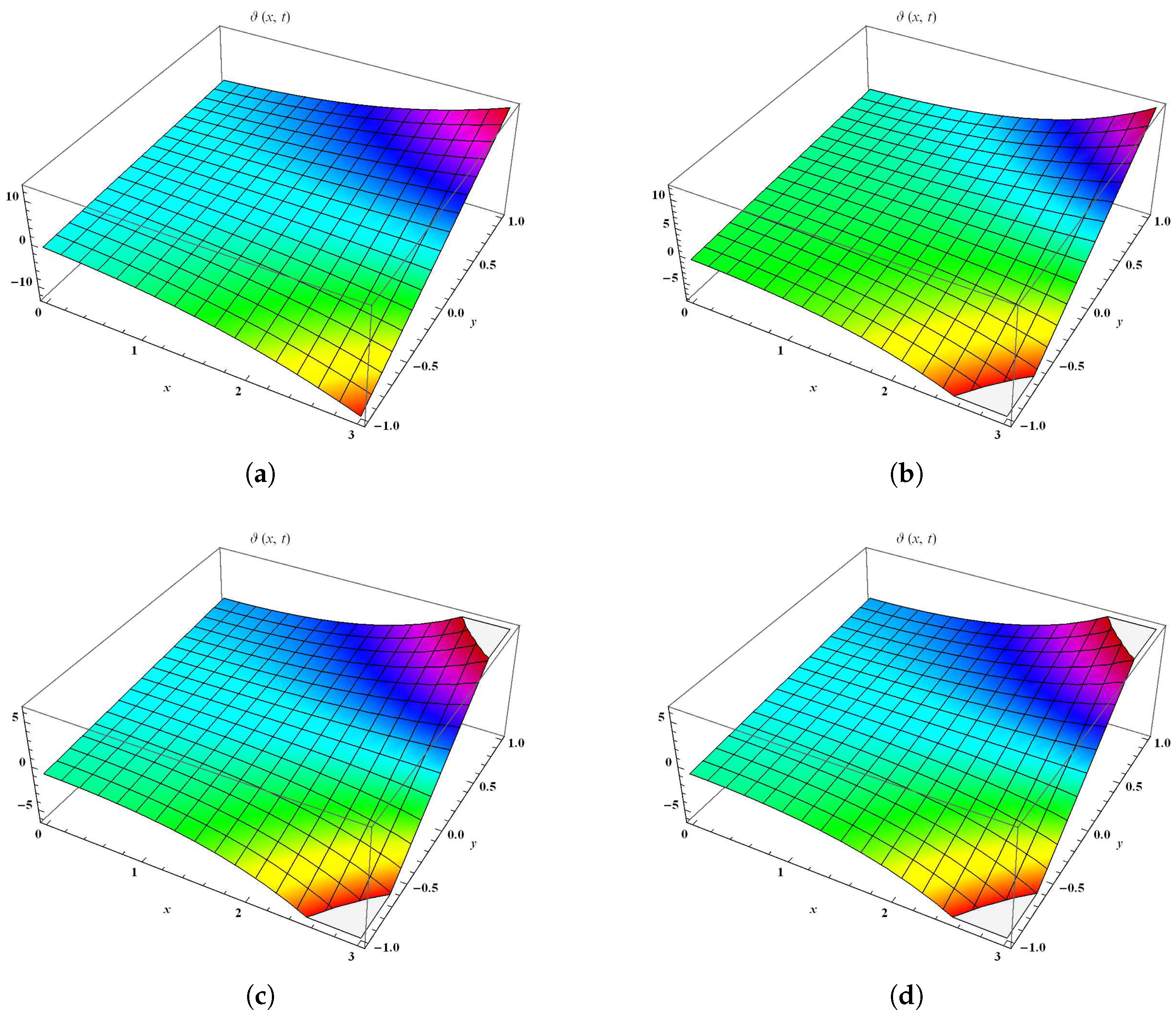
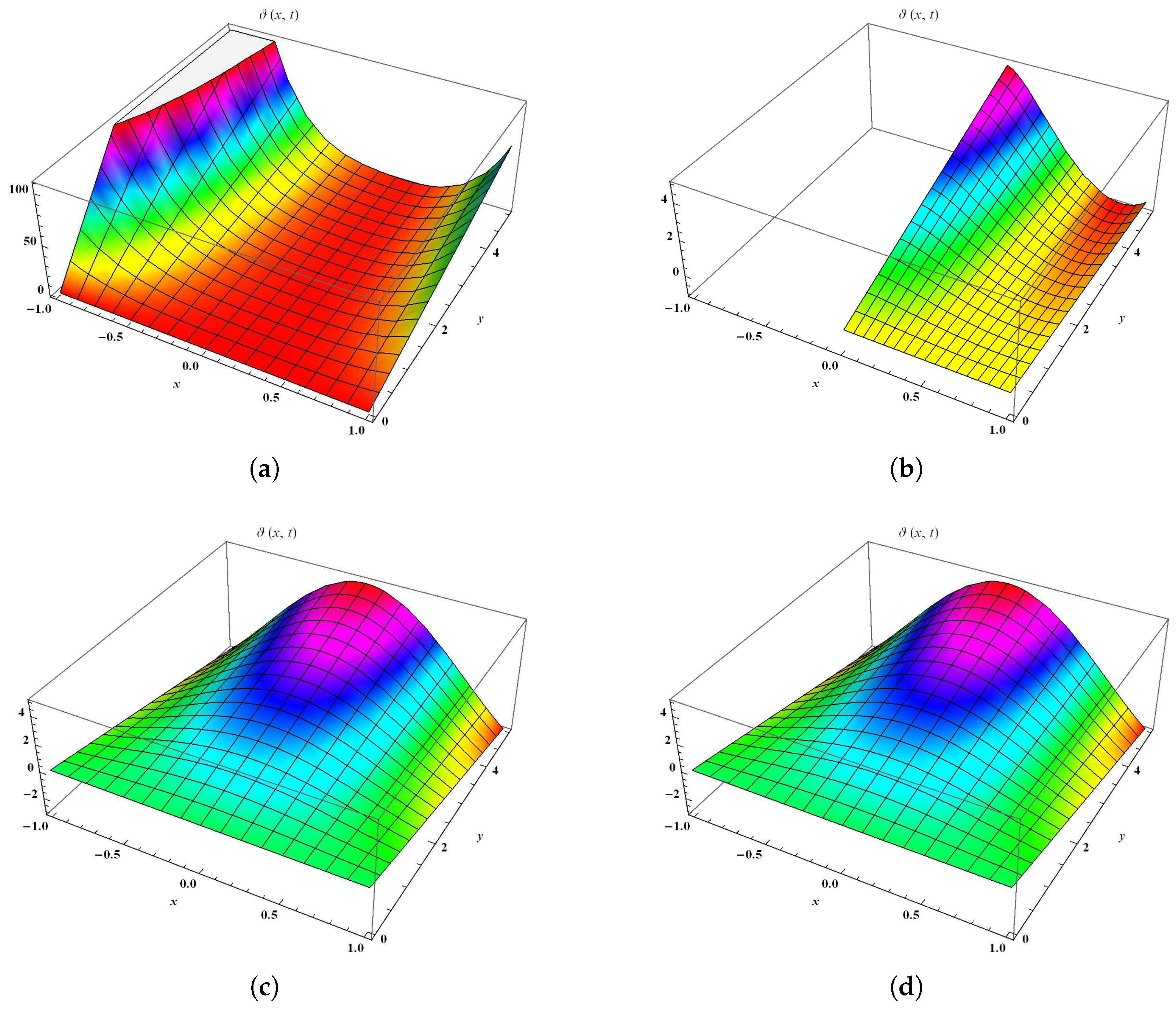
5. Description of Results

In this section, we explain the graphical results of fractional-order Helmholtz problems. Figure 1 has been divided into four sections at different fractional orders and considers the values 0 ς 3 and 1 τ 1 . Figure 1a,b shows the solution of the S T-RPSM at fractional orders α = 1 and 1.5 , respectively. Figure 1c provides the solution of the S T-RPSM at fractional order 2, whereas Figure 1d represents the graphical results of the exact solution. We observed that the graphical results of the S T-RPSM and the exact solution strongly agreed with each other. Table 1 provides the absolute error between the S T-RPSM and the exact solution at α = 1 , 1.5 , 2 . The results obtained by the S T-RPSM at fractional order α = 2 are in full agreement with the exact solution. We note that the absolute error decreased with a decrease in the values of ς and τ .
Similarly, Figure 2 has been divided into four sections at different fractional orders and considers the values 1 ς 1 and 0 τ 5 . Figure 2a,b shows the solution of the S T-RPSM at fractional orders α = 1 and 1.5 , respectively. Figure 2c shows the solution of the S T-RPSM at fractional order 2, whereas Figure 2d represents the graphical results of the exact solution. We observed that the graphical results of the S T-RPSM and the exact solution strongly agreed with each other. Table 2 shows the absolute error between the S T-RPSM and the exact solution at α = 1 , 1.5 , 2 . The results obtained by th S T-RPSM at fractional order α = 2 were in full agreement with the exact solution. We note that the absolute error decreased with a decrease in the values of ς and τ .

6. Conclusions

In this work, we developed the idea of the S T-RPSM and obtained an approximate solution for two-dimensional fractional Helmholtz problems. The obtained results were independent of any assumption that led to the exact solution very rapidly. We presented some graphical results in different fractional orders and computed the error estimate between the S T-RPSM and the exact solution. These results demonstrated that the S T-RPSM is accurate and valid for fractional order problems. We noticed that the S T-RPSM did not require much computational work and was easier to implement than other schemes. We conclude that our scheme is well developed and produces iterative series very swiftly. In the future, we plan to implement this approach for fractal problems and show how this approach is applicable to other nonlinear problems arising in science and engineering phenomena.

Author Contributions

Investigation and methodology, J.L.; software and writing—original draft, M.N.; validation and visualization, A.I.; conceptualization and formal analysis, S.M.; project management and funding acquisition, L.F.I. supervision, L.F.I. All authors have read and agreed to the published version of the manuscript.

Funding

This article was supported by the University of Oradea.

Data Availability Statement

Data are contained within the article.

Conflicts of Interest

The authors declare no conflict of interest.

References

  1. Ayasrah, M.; Al-Smadi, M.; Al-Omari, S.; Baleanu, D.; Momani, S. Structure of optical soliton solution for nonlinear resonant space-time Schrödinger equation in conformable sense with full nonlinearity term. Phys. Scr. 2020, 95, 105215. [Google Scholar]
  2. Al-Smadi, M.; Arqub, O.A. Computational algorithm for solving fredholm time-fractional partial integrodifferential equations of dirichlet functions type with error estimates. Appl. Math. Comput. 2019, 342, 280–294. [Google Scholar] [CrossRef]
  3. Khan, H.; Liao, S.J.; Mohapatra, R.; Vajravelu, K. An analytical solution for a nonlinear time-delay model in biology. Commun. Nonlinear Sci. Numer. Simul. 2009, 14, 3141–3148. [Google Scholar] [CrossRef]
  4. Gu, Y.; Liao, W.; Zhu, J. An efficient high-order algorithm for solving systems of 3-D reaction–diffusion equations. J. Comput. Appl. Math. 2003, 155, 1–17. [Google Scholar] [CrossRef]
  5. Alaje, A.I.; Olayiwola, M.O.; Adedokun, K.A.; Adedeji, J.A.; Oladapo, A.O. Modified homotopy perturbation method and its application to analytical solitons of fractional-order Korteweg–de Vries equation. Beni-Suef Univ. J. Basic Appl. Sci. 2022, 11, 139. [Google Scholar] [CrossRef]
  6. Arikoglu, A.; Ozkol, I. Solution of fractional differential equations by using differential transform method. Chaos Solitons Fractals 2007, 34, 1473–1481. [Google Scholar] [CrossRef]
  7. Nadeem, M.; Yao, S.W. Solving the fractional heat-like and wave-like equations with variable coefficients utilizing the Laplace homotopy method. Int. J. Numer. Methods Heat Fluid Flow 2020, 31, 273–292. [Google Scholar] [CrossRef]
  8. Akinyemi, L.; Iyiola, O.S. Exact and approximate solutions of time-fractional models arising from physics via Shehu transform. Math. Methods Appl. Sci. 2020, 43, 7442–7464. [Google Scholar] [CrossRef]
  9. Kumar, S.; Gupta, V. An application of variational iteration method for solving fuzzy time-fractional diffusion equations. Neural Comput. Appl. 2021, 33, 17659–17668. [Google Scholar] [CrossRef]
  10. Singh, H. Jacobi collocation method for the fractional advection-dispersion equation arising in porous media. Numer. Methods Partial. Differ. Equ. 2022, 38, 636–653. [Google Scholar] [CrossRef]
  11. Sartanpara, P.P.; Meher, R. A robust computational approach for Zakharov-Kuznetsov equations of ion-acoustic waves in a magnetized plasma via the Shehu transform. J. Ocean. Eng. Sci. 2021, 8, 79–90. [Google Scholar] [CrossRef]
  12. Yuttanan, B.; Razzaghi, M.; Vo, T.N. Legendre wavelet method for fractional delay differential equations. Appl. Numer. Math. 2021, 168, 127–142. [Google Scholar] [CrossRef]
  13. Veeresha, P.; Prakasha, D.; Singh, J. Solution for fractional forced KdV equation using fractional natural decomposition method. AIMS Math. 2020, 5, 798–810. [Google Scholar] [CrossRef]
  14. Tandel, P.; Patel, H.; Patel, T. Tsunami wave propagation model: A fractional approach. J. Ocean. Eng. Sci. 2022, 7, 509–520. [Google Scholar] [CrossRef]
  15. Prakasha, D.; Veeresha, P.; Baskonus, H.M. Residual power series method for fractional Swift–Hohenberg equation. Fractal Fract. 2019, 3, 9. [Google Scholar] [CrossRef]
  16. Hassani, H.; Machado, J.T.; Naraghirad, E. Generalized shifted Chebyshev polynomials for fractional optimal control problems. Commun. Nonlinear Sci. Numer. Simul. 2019, 75, 50–61. [Google Scholar] [CrossRef]
  17. El-Sayed, S.M.; Kaya, D. Comparing numerical methods for Helmholtz equation model problem. Appl. Math. Comput. 2004, 150, 763–773. [Google Scholar] [CrossRef]
  18. Momani, S.; Abuasad, S. Application of He’s variational iteration method to Helmholtz equation. Chaos Solitons Fractals 2006, 27, 1119–1123. [Google Scholar] [CrossRef]
  19. Gupta, P.K.; Yildirim, A.; Rai, K. Application of He’s homotopy perturbation method for multi-dimensional fractional Helmholtz equation. Int. J. Numer. Methods Heat Fluid Flow 2012, 22, 424–435. [Google Scholar] [CrossRef]
  20. Iqbal, N.; Chughtai, M.T.; Shah, N.A. Numerical simulation of fractional-order two-dimensional Helmholtz equations. AIMS Math. 2023, 8, 13205–13218. [Google Scholar] [CrossRef]
  21. Alshammari, S.; Abuasad, S. Exact solutions of the 3D fractional helmholtz equation by fractional differential transform method. J. Funct. Spaces 2022, 2022, 7374751. [Google Scholar] [CrossRef]
  22. Khater, M.M. Computational simulations of the cubic-quintic nonlinear Helmholtz model. J. Ocean Eng. Sci. 2022. [Google Scholar] [CrossRef]
  23. Arqub, O.A. Series solution of fuzzy differential equations under strongly generalized differentiability. J. Adv. Res. Appl. Math. 2013, 5, 31–52. [Google Scholar] [CrossRef]
  24. Aggarwal, S.; Gupta, A.R. Shehu transform for solving Abel’s integral equation. J. Emerg. Technol. Innov. Res. 2019, 6, 101–110. [Google Scholar]
  25. Khan, H.; Farooq, U.; Shah, R.; Baleanu, D.; Kumam, P.; Arif, M. Analytical solutions of (2+ time fractional order) dimensional physical models, using modified decomposition method. Appl. Sci. 2019, 10, 122. [Google Scholar] [CrossRef]
  26. Zhang, R.; Shah, N.A.; El-Zahar, E.R.; Akgül, A.; Chung, J.D. Numerical analysis of fractional-order emden–fowler equations using modified variational iteration method. Fractals 2023, 31, 2340028. [Google Scholar] [CrossRef]
  27. Saadeh, R.; Ala’yed, O.; Qazza, A. Analytical solution of coupled hirota–satsuma and KdV equations. Fractal Fract. 2022, 6, 694. [Google Scholar] [CrossRef]
  28. Kumar, A.; Kumar, S.; Singh, M. Residual power series method for fractional Sharma-Tasso-Olever equation. Commun. Numer. Anal. 2016, 10, 1–10. [Google Scholar] [CrossRef]
  29. El-Ajou, A.; Arqub, O.A.; Zhour, Z.A.; Momani, S. New results on fractional power series: Theories and applications. Entropy 2013, 15, 5305–5323. [Google Scholar] [CrossRef]
  30. Abuasad, S.; Moaddy, K.; Hashim, I. Analytical treatment of two-dimensional fractional Helmholtz equations. J. King Saud-Univ.-Sci. 2019, 31, 659–666. [Google Scholar] [CrossRef]
Figure 1. The 3D comparisons of S T-RPSM’s solutions of ϑ ( ς , τ ) in ς -space at various fractional orders with the exact solution. (a) The 3D S T-RPSM solution of ϑ ( ς , τ ) in ς -space at α = 1 ; (b) the 3D S T-RPSM solution of ϑ ( ς , τ ) in ς -space at α = 1.5 ; (c) the 3D S T-RPSM solution of ϑ ( ς , τ ) in ς -space at α = 2 ; (d) the 3D exact solution of ϑ ( ς , τ ) in ς -space.
Symmetry 15 02152 g001
Figure 2. The 3D comparisons of S T-RPSM’s solutions of ϑ ( ς , τ ) in ς -space at various fractional orders with the exact solution. (a) The 3D S T-RPSM solution of ϑ ( ς , τ ) in ς -space at α = 1 ; (b) the 3D S T-RPSM solution of ϑ ( ς , τ ) in ς -space at α = 1.5 ; (c) the 3D S T-RPSM solution of ϑ ( ς , τ ) in ς -space at α = 2 ; (d) the 3D exact solution of ϑ ( ς , τ ) in ς -space.
Symmetry 15 02152 g002
Table 1. Error estimates among the S T-RPSM’s results and the exact results of ϑ ( ς , τ ) in ς -space at various fractional orders for Example 1.
( ς , τ ) S T-RPSM S T-RPSM S T-RPSMExact ResultsAbsolute Error
α = 1 α = 1.5 α = 2
(0.05, 0.05)0.05256360.5042160.05006770.050067700000
(0.10, 0.10)0.1105170.1023960.10050.100500000
(0.15, 0.15)0.1742750.156640.1516910.15169100000
(0.20, 0.20)0.244280.2137260.2040130.20401300000
(0.25, 0.25)0.3210040.2741680.2578530.25785300000
(0.30, 0.30)0.4049510.3384580.3136020.31360200000
(0.35, 0.35)0.4966570.4070790.3716570.37165700000
(0.40, 0.40)0.5966930.4805150.4324290.43242900000
(0.45, 0.45)0.7056660.5592630.4963370.49633700000
(0.50, 0.50)0.8242190.643830.5638130.56381300000
Table 2. Error estimates among the S T-RPSM’s results and the exact results of ϑ ( ς , τ ) in ς -space at various fractional orders for Example 2.
( ς , τ ) S T-RPSM S T-RPSM S T-RPSMExact ResultsAbsolute Error
α = 1 α = 1.5 α = 2
(0.05, 0.05)0.03894040.4792330.04968780.049687800000
(0.10, 0.10)0.06067710.0885150.09751040.097510400000
(0.15, 0.15)0.07111820.1192640.1416410.14164100000
(0.20, 0.20)0.0750.1390520.1803310.18033100000
(0.25, 0.25)0.07686360.1476230.2119440.21194400000
(0.30, 0.30)0.08203130.145350.2349940.23499400000
(0.35, 0.35)0.0975830.1330780.2481730.24817300000
(0.40, 0.40)0.1333330.11210.2503860.25038600000
(0.45, 0.45)0.2028080.08360750.2407720.24077200000
(0.50, 0.50)0.3242190.04952440.2187260.21872600000
Disclaimer/Publisher’s Note: The statements, opinions and data contained in all publications are solely those of the individual author(s) and contributor(s) and not of MDPI and/or the editor(s). MDPI and/or the editor(s) disclaim responsibility for any injury to people or property resulting from any ideas, methods, instructions or products referred to in the content.

