The Continuous Measure of Symmetry as a Dynamic Variable: A New Glance at the Three-Body Problem

Abstract

The time evolution of the continuous measure of symmetry for a system built of three bodies interacting via the potential $U\left(r\right)~\frac{1}{r}$ is reported. Gravitational and electrostatic interactions between the point bodies were addressed. In the case of a pure gravitational interaction, the three-body-system deviated from its initial symmetrical location, described by the Lagrange equilateral triangle, comes eventually to collapse, accompanied by the growth of the continuous measure of symmetry. When three point bodies interact via the repulsive Coulomb interaction, the time evolution of the CMS is quite different. The CMS calculated for all of the studied initial configurations of the point charges, and all of their charge-to-mass ratios, always comes to its asymptotic value with time, evidencing the stabilization of the shape of the triangle, constituted by the interacting bodies. The influence of Stokes-like friction on the change in symmetry of three-body gravitating systems is elucidated; the Stokes-like friction slows the decrease in the CMS and increases the stability of the Lagrange triangle.

1. Introduction

In the three-body problem, three bodies/masses move in 3D space due to their gravitational interactions, as described by Newton’s law of gravity [1]. Solutions to this problem require that the future and past motions of the bodies be uniquely determined based solely on their present positions and velocities [1,2]. In the general case, the motions of the interacting bodies take place in three dimensions (3D), and there are no restrictions on their masses nor on their initial conditions. This problem is referred as “the general three-body problem” [1,2,3]. Unlike two-body problems, no general closed-form solution of the three-body problem exists. The behavior of three-body dynamical systems is chaotic for most initial conditions, and numerical methods are generally required for deriving the trajectories of the involved masses. In a restricted number of special configurations of the bodies, the exact solutions of the problem do exist. A special case of the three-body problem was analyzed by Euler [1,2,3]. Euler considered three bodies of arbitrary (finite) masses and placed them along a straight line. Euler demonstrated that the bodies would always stay on the same straight line for suitable initial conditions, and that the line would rotate about the center of mass of the system, resulting in periodic motions of all three bodies along ellipses [1,2,3]. Lagrange considered an equilateral triangle configuration of the three bodies, and demonstrated that, in this case, the bodies also move along elliptic orbits [1,2,3]. In the Lagrange solution, the initial configuration is an equilateral triangle and the three bodies are located at its vertices. We demonstrate that the “Lagrange equilateral triangle” enables the straightforward introducing of the continuous measure of symmetry to the analysis of the three-body problem. Lagrange proved that for suitable initial conditions, the triangular configuration is maintained, and that the trajectories of the three bodies remain elliptical within the motion [1,2,3]. This great progress in the development of the three-body problem is related to the fundamental studies by Henri Poincaré [4]. Poincaré and Bendixson studied the conditions giving rise to the existence of periodic solutions in the three-body problem [4].

The three-body problem remains one of the “evergreen” problems of physics. Novel ideas were successfully applied for the solution of the problem. In particular, deep artificial neural networks (abbreviated as ANNs) were involved in the solution of the problem [5]. It was demonstrated that for computationally challenging regions of phase space, a trained ANN can replace existing numerical solvers, enabling the fast and scalable simulations of many-body systems [5]. The relativistic Pythagorean three-body problem was addressed recently (within this problem, three bodies with masses 3, 4, and 5 are positioned at rest in a planar, right-angled triangle at positions (1, 3), (−1, −2), and (1, −1), respectively) [6]. Dissipative effects, through gravitational wave emission, were considered [6]. A statistical, approximate solution of the bound, nonhierarchical three-body problem was reported (instead of predicting the actual outcome, the authors calculated the probability of any given outcome of interactions between the bodies) [7]. Periodic collisionless equal-mass free-fall orbits were elucidated [8].

Our paper presents a new approach to the three-body problem, based on the application of the continuous measure of symmetry (abbreviated as CMS) to the problem. It seems that the first successful symmetrization of the equations of the three-body problem was performed by Broucke and Lass in 1973 [9]. It was demonstrated that the equations of the general three-body problem take on a very symmetric form when one considers only their relative positions, rather than their position vectors relative to some given coordinate system [9]. From these equations one quickly derives some well-known classical properties of the three-body problem, such as the first integrals and the equilateral triangle solutions [9]. We demonstrate the possibility of applying the recently introduced CMS to the analysis of the three-body problem. The symmetry is usually considered within a binary paradigm; simply and roughly speaking, symmetry is present or absent in a given physical system. This YES/NO binary paradigm has been broken by introducing the continuous measure of symmetry based on the symmetry distance of the shape, which was introduced by Zabrodsky, Peleg, and Avnir in the 90s [10,11,12,13,14]. The symmetry distance of the shape is defined as the minimum mean square distance required to move the points of the original shape in order to obtain a symmetrical shape [10,11,12,13,14,15]. Successful applications of the CMS to the analysis of physical problems is demonstrated [16,17,18,19].

2. Materials and Methods

Computer simulations were carried out with the software “Taylor Center”, version 42; http://taylorcenter.org/Gofen/TaylorMethod.htm [20,21], accessed on 1 January 2023.

This software is an advanced ordinary differential equations solver implementing the modern Taylor integration method (Automatic Differentiation) in a multi-functional user-friendly environment with unique features such as graphing and real-time animation of the trajectories in 2D and 3D stereo, and with the highest number of significant digits—the Intel extended 10 byte format with 63-bit mantissa (19 decimal digits). The demo version of the “Taylor Center” software is free of charge [20,21].

3. Results and Discussion

3.1. The Continuous Measure of Symmetry and Its Calculation

Let us become acquainted with the continuous measure of symmetry, as it was defined and developed by Zabrodsky, Peleg, and Avnir [10,11,12,13,14]. Consider a non-symmetrical shape consisting of $p$ points $M_i$, $\left(i=1, 2\dots n_p\right)$ and a given symmetry group, denoted as $\tilde{G}$. The continuous symmetry measure, labeled CMS and denoted as $S\left(\tilde{G}\right),$ is determined by the minimal average square displacement of the points, $M_i$, that the shape has to undergo in order to acquire the prescribed G-symmetry; seen as the minimum effort required to transform a given shape into a symmetrical shape. Rigorously speaking, the symmetry measure of the $\tilde{G}$-symmetry point group’s content $S\left(\tilde{G}\right)$ of an object is a function of the distance between the original structure and a searched $\tilde{G}$-symmetric reference structure; of the same point objects and connectivity, and which is the closest to the original distorted structure [10,11,12,13,14,15,16,17,18,19].

Assume that the $\tilde{G}$-symmetrical shape emerges from the set of points ${\widehat{M}}_i$. Since the set ${\widehat{M}}_i$ is established, a CMS is defined as

$$S\left(\tilde{G}\right)=\frac{1}{n_p{\tilde{R}}^2}{\displaystyle {\sum }_{i=1}^{n_p}}{\left|M_i-{\widehat{M}}_i\right|}^2,$$

(1)

where $\tilde{R}$ is the distance between the center of mass to the vertex of the closest equilateral triangle, which is used for the normalization of the CMS (the squared values in Equation (1) supply a function that is isotropic, continuous, and differentiable; it should be mentioned that after normalization 0 $<S\left(\tilde{G}\right)<1$ is true). The continuous measure of symmetry defined using Equation (1) is a dimensionless value. At the first step, the points of the nearest shape demonstrating the $\tilde{G}$-type symmetry must be established. An algorithm that identifies the set of points ${\widehat{M}}_i$ that constitute this symmetrical shape was introduced in [6,7,8,9,10,11]. Figure 1 depicts an equilateral triangle${ M}_{01}{M}_{02}{M}_{03}$ representing the symmetric shape that corresponds to the given non-symmetric triangle ${ M}_1{M}_2{M}_3$.

The transformation of the non-symmetric triangle ${ M}_1{M}_2{M}_3$ to the symmetric equilateral triangle ${ M}_{01}{M}_{02}{M}_{03}$ is performed as follows: vertex $M_i$ is rotated counterclockwise around the common centroid $O$ of triangle ${ M}_1{M}_2{M}_3$ by $\frac{2\pi (i-1)}{3}$ radians (one vertex of triangle ${ M}_1{M}_2{M}_3$ remains fixed); thus, triangle $M_1{M}_2^{\prime }{M}_3^{\prime }$ emerges. Next, the location of the centroid $O^{\prime }$ of the intermediate triangle $M_1{M}_2^{\prime }{M}_3^{\prime }$ is determined. Centroid $O^{\prime }$is then rotated clockwise around the centroid $O$ by $-\frac{2\pi (i-1)}{3}$ radians (for the details see [14]).

Therefore, the equilateral triangle ${ M}_{01}{M}_{02}{M}_{03}$ shown in Figure 1 represents the closest symmetrical shape to the pristine non-symmetrical triangle ${ M}_1{M}_2{M}_3$ [6,7,8,9,10,11,12,13,14]. Since the set ${\widehat{M}}_i$ is established, the CMS is calculated using Equation (1) (the importance of the normalization procedure should be emphasized). The equilateral Lagrange triangle supplying the solution to the three-body problem hints to the effectiveness of the use of CMS for the solution of the three-body problem [1,2].

3.2. Symmetrized Equations of Motion for the Three-Body Problem

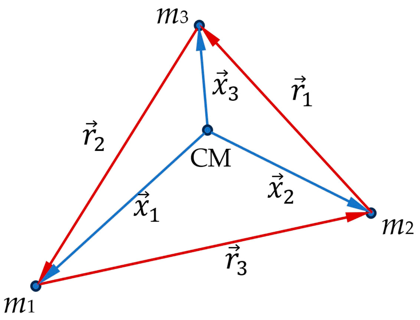
Consider the three-body problem for a set of three gravitating masses $m_i, i=1\dots 3.$ In the center-of-mass frame, the equations of motion of the point gravitating masses appear as follows:

$$\overrightarrow{{\ddot{\mathrm{x}}}_i}=-G{m}_j\frac{{\overrightarrow{x}}_i-{\overrightarrow{x}}_j}{{\left|{\mathrm{x}}_i-{\mathrm{x}}_j\right|}^3}-G{m}_k\frac{{\overrightarrow{x}}_i-{\overrightarrow{x}}_k}{{\left|{\mathrm{x}}_i-{\mathrm{x}}_k\right|}^3}, i,j,k=1, 2, 3),$$

(2)

where $x_i,x_j ,x_k\left(i, j,k=1\dots 3\right)$ are the coordinates of the masses in the center-of-mass frame defined by $\sum _{i=1}^{i=3}{m}_i{\overrightarrow{x}}_i$=0; $\frac{d}{dt}\sum _{i=1}^{i=3}{m}_i{\overrightarrow{x}}_i$=0, as illustrated in Figure 2, and G is the gravitational constant.

Broucke and Lass suggested the procedure of symmetrization of Equation (2), with the use of the vectors of the relative locations of the masses, ${\overrightarrow{r}}_i={\overrightarrow{x}}_j-{\overrightarrow{x}}_k$ (vector ${\overrightarrow{r}}_i$ corresponds to the side opposite the apex of the triangle occupied by mass $m_i$, see Figure 2). Equation (3) is obviously true for vectors ${\overrightarrow{r}}_i \left[9\right]$

$${\displaystyle {\sum }_{i=1}^3}{\overrightarrow{r}}_i=0$$

(3)

Introducing vectors ${\overrightarrow{r}}_i$ yields the equations of motion re-shaped and symmetrized as follows:

$${\overrightarrow{\ddot{r}}}_i=-G\left(M\frac{{\overrightarrow{r}}_i}{r_i^3}-m_i\overrightarrow{R}\right),$$

(4)

where $M=\sum _{i=1}^3{m}_i$ is the total mass of the system and vector $\overrightarrow{R}$ is defined by Equation (5):

$$\overrightarrow{R}={\displaystyle {\sum }_{i=1}^3}\frac{{\overrightarrow{r}}_i}{r_i^3},$$

(5)

The first term in Equation (4) is identical to that appearing in the standard two-body Kepler problem, whereas the second term in Equation (4) generates the complexity of the evergreen three-body problem. The Lagrange solution of the problem corresponds to the case when r₁ = r₂ = r₃ takes place. In this situation $\overrightarrow{R}=0$ is true. Thus, the three-body problem is reduced to the two-body one, and the gravitating masses remain in the vertices of an equilateral triangle. The triangle may change its size and rotate; gravitating masses are moving along ellipses with different eccentricities; however, they are oriented at different angles to one another [22]. The motion of the gravitating masses in this case is periodic, with the same period for all of the masses. It should be emphasized that the aforementioned Lagrange solution remains stable only if one of the masses is much larger than other two [23,24].

3.3. Extension of the Problem to the Coulomb Interaction

Consider the system of three point charges $q_i, i=1, 2, 3$ possessing the corresponding masses $m_i, i=1, 2, 3$. For a sake of simplicity, we assume that the motion of the point charges is slow; thus, the electrodynamic interaction between the charges may be neglected and only the electrostatic and gravitational interactions between the bodies are essential. We consider the case in which the initial velocities of the interacting bodies are zero; thus, our approach will be true at least at the initial stage of the motion, when the velocities of the bodies are still small (very roughly speaking, it is true when $\frac{v}{c}\ll 1$ is true, where v is the velocity of the charge and c is the velocity of light in a vacuum). The vector equations of motion in this non-relativistic case appear as follows:

$${\overrightarrow{\ddot{\mathrm{x}}}}_i=-(G{m}_j-\frac{K}{m_i}{q}_i{q}_j)\frac{{\overrightarrow{x}}_i-{\overrightarrow{x}}_j}{{\left|x_i-x_j\right|}^3}-(G{m}_k-\frac{K}{m_i}{q}_i{q}_k)\frac{{\overrightarrow{x}}_i-{\overrightarrow{x}}_k}{{\left|x_i-x_k\right|}^3},$$

(6)

where K is the Coulomb constant. To make the problem even more simple, we also assume $G{m}_j\ll \frac{K}{m_i}{q}_i{q}_j$ and, thus, the gravitational interaction is negligible (obviously, this case has nothing to do with celestial mechanics); this simple case yields interesting and understandable results. Hence, the equation of motion is re-written as follows:

$${\overrightarrow{\ddot{\mathrm{x}}}}_i=\frac{K}{m_i}{q}_i{q}_j\frac{{\overrightarrow{x}}_{\mathrm{i}}-{\overrightarrow{x}}_j}{{\left|x_i-x_j\right|}^3}+\frac{K}{m_i}{q}_i{q}_k\frac{{\overrightarrow{x}}_i-{\overrightarrow{x}}_k}{{\left|x_i-x_k\right|}^3}$$

(7)

The symmetrical coordinates introduced and discussed in detail in the previous section yield, in turn, Equation (8) [9]:

$${\overrightarrow{\ddot{r}}}_i=K\left[\left(\frac{q_i}{m_i}{q}_j+\frac{q_j}{m_j}{q}_i+\frac{q_k}{m_k}{q}_k\right)\frac{{\overrightarrow{r}}_i}{r_i^3}-q_i\left(\frac{q_i}{m_i}\frac{{\overrightarrow{r}}_j}{r_j^3}+\frac{q_j}{m_j}\frac{{\overrightarrow{r}}_i}{r_i^3}+\frac{q_k}{m_k}\frac{{\overrightarrow{r}}_k}{r_j^3}\right)\right], i,j,k=1\dots 3,$$

(8)

In the case where $\raisebox{1ex}{$q_1$}\!\left/ \!\raisebox{-1ex}{$m_1$}\right.=\raisebox{1ex}{$q_2$}\!\left/ \!\raisebox{-1ex}{$m_2$}\right.=\raisebox{1ex}{$q_3$}\!\left/ \!\raisebox{-1ex}{$m_3$}\right.=\mu$ takes place, we obtain this from Equations (8) and (9), which resembles Equation (4), namely:

$${\overrightarrow{\ddot{r}}}_i=K\mu \left(Q\frac{{\overrightarrow{r}}_i}{r_i^3}-q_i\overrightarrow{R}\right),$$

(9)

where $Q=\sum _{i=1}^3{q}_i$ is the total electrical charge of the system and vector $\overrightarrow{R}$ is defined using Equation (5). Equation (9) immediately leads to the conclusion that the solution of the three-body problem, similar to that suggested by Lagrange, exists in the case when the interaction between the bodies is the pure electrostatic/Coulomb one. The Lagrange triangle appears as a solution of the three-body problem when the electrical charges of the same sign are initially placed in the vertices of an equilateral triangle, and the condition $\raisebox{1ex}{$q_1$}\!\left/ \!\raisebox{-1ex}{$m_1$}\right.=\raisebox{1ex}{$q_2$}\!\left/ \!\raisebox{-1ex}{$m_2$}\right.=\raisebox{1ex}{$q_3$}\!\left/ \!\raisebox{-1ex}{$m_3$}\right.=\mu =const$takes place.

3.4. Considering Friction and Dissipative Processes

Now we consider the impact of the dissipative forces on the time evolution of the CMS.

Assume that the Stokes-like friction force ${\overrightarrow{F}}_{fr}$ acts on the interacting bodies, i.e., ${\overrightarrow{F}}_{fr}$ = −$b_i{\overrightarrow{\dot{x}}}_i$ takes place, where $b_i$ is the friction factor and ${\dot{x}}_i$ is the velocity of i-th body. Generally speaking, the friction factors may be various for the different interacting bodies. Equation (6), considering the friction force, yields Equation (10):

$${\overrightarrow{\ddot{\mathrm{x}}}}_i=-(G{m}_j-\frac{K}{m_i}{q}_i{q}_j)\frac{{\overrightarrow{\mathit{x}}}_i-{\overrightarrow{x}}_j}{{\left|x_i-x_j\right|}^3}-(G{m}_k-\frac{K}{m_i}{q}_i{q}_k)\frac{{\overrightarrow{x}}_i-{\overrightarrow{x}}_k}{{\left|x_i-x_k\right|}^3}-\frac{b_i}{m_i}{\overrightarrow{\dot{x}}}_i,$$

(10)

Thus, Equation (2) is re-shaped as follows:

$${\overrightarrow{\ddot{\mathrm{x}}}}_i=-G{m}_j\frac{{\overrightarrow{\mathit{x}}}_i-{\overrightarrow{x}}_j}{{\left|x_i-x_j\right|}^3}-G{m}_k\frac{{\overrightarrow{x}}_i-{\overrightarrow{x}}_k}{{\left|x_i-x_k\right|}^3}-\frac{b_i}{m_i}{\overrightarrow{\dot{x}}}_i,$$

(11)

Vector ${\overrightarrow{\ddot{r}}}_i={\overrightarrow{\ddot{x}}}_j-{\overrightarrow{\ddot{x}}}_k$ is re-written as Equation (12) (similarly to Equation (4)):

$${\overrightarrow{\ddot{r}}}_i=-G\left(M\frac{{\overrightarrow{r}}_i}{r_i^3}-m_i\overrightarrow{R}\right)-\left(\frac{b_j}{m_j}{\overrightarrow{\dot{x}}}_j-\frac{b_k}{m_k}{\overrightarrow{\dot{x}}}_k\right),$$

(12)

We assume b₁/m₁ = b₂/m₂ = b₂/m₂ = const = γ; thus, the second term in Equation (12) appears as follows:

$$\left(\frac{b_j}{m_j}{\overrightarrow{\dot{x}}}_j-\frac{b_k}{m_k}{\overrightarrow{\dot{x}}}_k\right)=\gamma \left({\overrightarrow{\dot{x}}}_j-{\overrightarrow{\dot{x}}}_k\right)=-\gamma {\overrightarrow{\dot{r}}}_i,$$

(13)

and we derive Equation (14), resembling Equation (4). However, considering the dissipative friction forces:

$${\overrightarrow{\ddot{r}}}_i=-G\left(M\frac{{\overrightarrow{r}}_i}{r_i^3}-m_i\overrightarrow{R}\right)+\gamma {\overrightarrow{\dot{r}}}_i,$$

(14)

when the bodies are initially located in the vertices of the equilateral triangle $\overrightarrow{R}=0$, and consequently we derive

$${\overrightarrow{\ddot{r}}}_i=-GM\frac{{\overrightarrow{r}}_i}{r_i^3}+\gamma {\overrightarrow{\dot{r}}}_i,$$

(15)

In parallel to Equation (14), we obtain, for the Coulomb interactions, Equation (16):

$${\overrightarrow{\ddot{r}}}_i=K\mu \left(Q\frac{{\overrightarrow{r}}_i}{r_i^3}-q_i\overrightarrow{R}\right)+\gamma {\overrightarrow{\dot{r}}}_i,$$

(16)

which resembles Equation (15) for the equilateral Lagrange triangle. Equation (15) is the second-order nonlinear ordinary differential equation. The exact solution of the three-body problem, considering the dissipation forces and similar to that suggested by Lagrange, exists only when the condition $\raisebox{1ex}{$b_1$}\!\left/ \!\raisebox{-1ex}{$m_1$}\right.=\raisebox{1ex}{$b_2$}\!\left/ \!\raisebox{-1ex}{$m_2$}\right.=\raisebox{1ex}{$b_3$}\!\left/ \!\raisebox{-1ex}{$m_3$}\right.$ is fulfilled and the condition $\overrightarrow{R}=0$ takes place. For a sake of simplicity, we consider in our treatment the case where b₁ = b₂= b₃ = b is true.

3.5. The Three-Body Problem and the Continuous Measure of Symmetry

The three-body problem in its general case has no analytical solution. We studied, with the computer simulations, the evolution of the continuous measure of symmetry of the three-body systems interacting via the Newtonian–Coulomb potential $U\left(r\right)~\frac{1}{r}$. We also considered the situations in which friction is present [7]. The initial location of the point bodies/charges was slightly shifted from their initial configuration, constituting the equilateral triangle (the so-called “Lagrange triangle”). Computer simulations were carried out with the software “Taylor Center”, version 42; http://taylorcenter.org/Gofen/TaylorMethod.htm [20,21], accessed on 1 January 2023.

Gravitational and Coulomb interactions were considered. In the first series of computer experiments, the displacement of bodies from their initial location was 5%, as shown in Figure 3. In the second series of the numerical experiments, the mass-to-charge ratio of the interacting particles was varied. In the third series of simulations, the location of the particles and their charge-to-mass ratio were varied simultaneously.

We start from the first series of computer experiments, in which pure gravitational interaction between the bodies is assumed. The displacement of the bodies from their initial location is illustrated in Figure 3; we shift the bodies along the coordinate axes. ${\delta }_1=0.05$ corresponds to the displacement of the mass $m_1$ to the right (in the positive direction of axis x), whereas ${\delta }_2=0.05$ corresponds to the displacement of the mass $m_1$ to the left (in the negative direction of axis x).

Simple combinatory analysis demonstrates that there exists in total 64 possibilities of the distortion of the initial equilateral triangle, when locations of all of the vertices are perturbed; we do not report here the exhaustive analysis of all of the possible deformations of the Lagrange triangle, as we are focused on some of the illustrative examples of the general three-body problem. In all of the cases, the continuous measure of symmetry (see Section 2) was taken as a dynamic variable, i.e., $S\left(t\right)$ was calculated, quantifying the distortion of the initial equilateral Lagrange triangle under the motion governed by gravitational or Coulomb forces (see Equations (4) and (9)). Consider Example #1, in which three bodies interact via a pure gravitational interaction, and $x_1=1.05$ is assumed, as shown in Figure 3 $(G=1$ is assumed for the sake of simplicity). The initial positions of the gravitating bodies are m₁(1.05, 0), m₂(cos(π/3), sin(π/3)), and m₃(cos(2π/3), sin(2π/3)); the initial velocities are zero and friction is absent, i.e., $b=0.$ The motion of two sets of dimensionless masses was analyzed, namely: m₁ = m₂= m₃ = 1 and m₁ = 3, m₂ = 4, m₃ = 5. The results of the calculations for both sets of masses are supplied in Figure 4.

Figure 4 reveals a number of very important qualitative conclusions: (i) Irrespective of the interrelation between the gravitating masses, the distortion of the Lagrange triangle destroys the symmetry of the systems and results in the gravitational collapse of the system; the situation $CMS=1$ corresponds to the disappearance of the one of the sides of the triangle, as will be shown below. (ii) The destruction of the symmetry is not immediate; systems demonstrate a certain stability until some threshold value of distortion. The calculation of this value needs additional physical and computational insights, which are not covered in the present paper. It is noteworthy that there exists a 3D extension of the Lagrange triangle, and it is the Lagrange tetrahedron, where four gravitating bodies are located at its vertices.

Now consider the impact of friction on the time evolution of the CMS. The initial positions of the gravitating bodies are m₁(1.05, 0), m₂(cos(π/3), sin(π/3)), and m₃(cos(2π/3), sin(2π/3)); the initial velocities are zero; the dimensionless friction factor is varied in the range $0<b<10.$ The motion of the two sets of dimensionless masses is analyzed, namely: m₁ = m₂= m₃ = 1. The results of the calculations for both sets of masses are supplied in Figure 5.

Again, we conclude that the distortion of the Lagrange triangle destroys the symmetry of the system and results in the gravitational collapse of the system; and this remains true in the presence of friction. An increase in friction shifts the degradation of symmetry in tim; in other words, friction, as it may be expected, increases the stability of the Lagrange triangle.

3.6. The Coulomb Interaction, the Three-Body Problem, and the Continuous Measure of Symmetry

Now we consider the slightly deformed Lagrange triangle $(x=1.05 \mathrm{a}\mathrm{n}\mathrm{d} x=0.95$ is true for one of the vertices). The point charges $q_i, i=1..3$ are located in the vertices of the triangle; the initial velocities of the charges are zero. We address the situation in which electrodynamic interactions are neglected, and the Coulomb interactions dominate over gravitational ones (the Coulomb constant is equaled to unity). The masses of the bodies and their charges are m₁ = m₂= m₃ = 1; q₁ = q₂ = q₃ = 1; and friction is absent, i.e., b = 0. The equations of motion are supplied by Equation (9). The results of the computer simulations, which establish the time evolution of the CMS, denoted $S\left(t\right),$ are supplied in Figure 6.

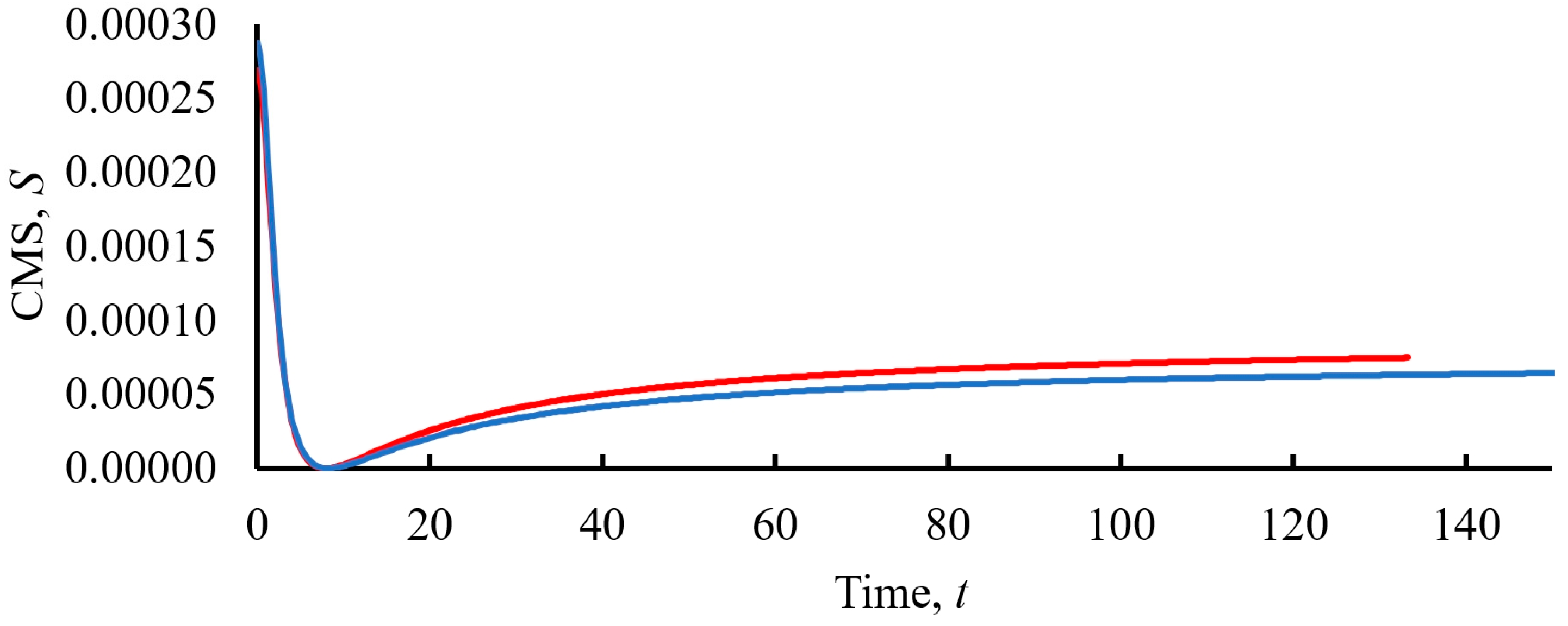
The time evolution of CMS demonstrates, in both of the cases, an identical behavior, which may be described as follows: the systems start with a non-zero value of the CMS (the initial Lagrange triangle is distorted); afterwards, the charges came to the vertices of the equilateral triangle (CMS equals zero, see Figure 6), and afterwards the CMS grew and attained an asymptotic value. This result is intuitively clear: consider that only the repulsive Coulomb forces act between the point charges; these forces are weakened over the course of motion of the charges; thus, the shape of the triangle constituted by the charges is stabilized, and consequently the CMS attains its asymptotic value. This non-obvious result is of primary importance, enabling the qualitative characterization of the configuration of the moving point charges. The charges come to the vertices of the equilateral triangle with non-zero velocities, and thus, they pass these points and continue to move, driven by the repulsive Coulomb forces, finally obtaining the configuration quantified by the asymptotic value of the CMS. We will demonstrate that the asymptotic behavior of the CMS is observed for various interrelations between the charges and masses of the interacting bodies.

Consider now the situation in which m₁ >> m₂= m₃ and q₁ >> q₂ = q₃ takes place. These conditions are similar to those inherent for the stable Lagrange solution of the three-body problem [1,2]. The time evolution of the continuous measure of symmetry for this case is depicted in Figure 7.

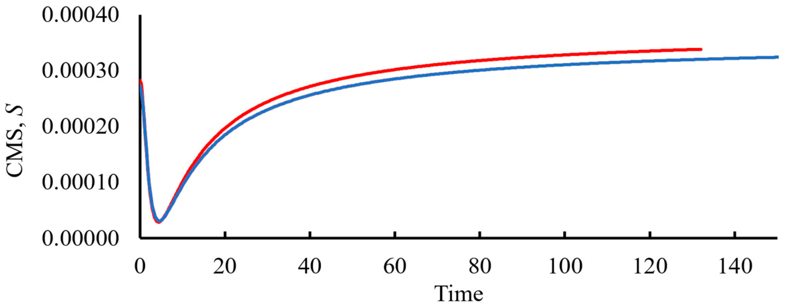
In this situation, the initial CMS is decreased over the course of motion of the electrically charged bodies, and it comes to its saturation value depending on the initial distortion of the Lagrange triangle, as shown in Figure 7. Again, only repulsive Coulomb interactions are present in the system; the Coulomb repulsion is decreased with time and eventually the CMS attains its saturation value, quantifying the distortion of the initial triangle.

We also varied, in our computer experiments, the charge of one of the point masses $(q_1=0.95, q_1=1.05$ were tested numerically). In these experiments the charges were placed in the vertices of the undistorted equilateral Lagrange triangle. The time evolution of the CMS is shown in Figure 8.

In this case, the initial value of the CMS is zero (the initial Lagrange triangle is equilateral). The value of the CMS grows over the course of motion of the charges and comes to saturation, as shown in Figure 8.

We also tested the situation in which the initial Lagrange triangle was slightly distorted and the charge-to-mass ratio of one of the charges was also slightly different from that prescribed for the other charges. The time evolution of the CMS in this case is shown in Figure 9.

The time evolution of the CMS in this case is similar to that shown in Figure 6, namely, the systems start with a non-zero value of the CMS (the initial Lagrange triangle is distorted); afterwards, the charges come to the vertices of the equilateral triangle with non-zero velocities (CMS equals zero, see Figure 9), and afterwards the CMS grows with time and attains its asymptotic value.

Now we perturb the geometrical symmetry and the charge-to-mass ratio for different vertices of the initial Lagrange triangle, namely, we assume x₁ = 1.05 and q₂ = 0.95 and x₁ = 0.95 and q₂ = 1.05; friction is absent, $b=0.$ The temporal evolution of the CMS is illustrated in Figure 10.

The time evolution of the CMS resembles qualitatively the behavior of the CMS depicted in Figure 9; however, the CMS does not attain zero as its minimal value, as it recognized from Figure 10.

The qualitative description of the change in the shape of the initial Lagrange triangle is illustrated in Figure 11, which supplies the main types of the time evolution of the Lagrange triangle.

Now we consider the situation already addressed in Figure 8, where the Stokes-like friction is taken into account. The time evolution of the CMS is shown in Figure 12.

The time evolution of the continuous measure of symmetry was calculated for the system of the point charges located in the vertices of the non-distorted equilateral Lagrange triangle. The friction factor was varied in the range $0.2<b<1$. We recognize, from Figure 12, that friction decreases the saturation value of the CMS, and this is intuitively well expected. It is also noteworthy that the increase in friction decreases the saturation values of the CMS; in other words, friction promotes more symmetrical eventual shapes in the addressed systems.

Now, similarly to the case addressed in Figure 9, we perturb the geometrical symmetry and, in parallel, we perturb the charge-to-mass ratio for different vertices of the initial Lagrange triangle, namely we assume m₁ = m₂= m₃ = 1, x₁ = 1.05, and q₁ = 1.05.

The friction factor is varied in the range $0<b<2.$ The temporal evolution of the CMS in this case is illustrated in Figure 13. In this case, two ranges of the friction factor are distinguished: namely, when $0<b<0.1,$ the saturation value of the CMS is decreased with the growth of b; in contrast (see Figure 13A), when 0.25 $<b<2,$ the saturation value of CMS is increased with the growth of b (see Figure 13B). The interpretation of this observation calls for additional insights.

Perhaps the most surprising and intriguing result was obtained for the friction factor restricted within the range of $0<b<0.12.$ This result is illustrated in Figure 14.

Somewhat surprisingly, for $0<b<0.12,$ the twin well-shaped time dependence of the CMS was observed, as depicted in Figure 14. This means that the perturbed triangle formed by the bodies twice comes to the equilateral Lagrangian shape. The origin of the twin well-shaped curve, depicted in Figure 14, calls for additional physical insights.

4. Discussion

It seems that the Coulomb and gravity interaction are well expected to exert a similar impact on the configuration of bodies in the three-body problem. It is demonstrated that this conclusion is wrong: the CMS is stabilized over the course of the Coulomb interaction between the bodies and comes with time to its asymptotic value, as shown in Figure 5, Figure 6, Figure 7, Figure 8 and Figure 9, which is impossible for the gravitational interaction. Contrastingly, the symmetry of gravitating systems demonstrates a certain stability until some threshold value of distortion; however, eventually it is destroyed, as shown in Figure 4. Friction, as it may be expected, increases the stability of the Lagrange triangle comprising the gravitating masses.

In our future investigations we plan to address the evolution of the CMS for the 3D, symmetric, initial configurations of bodies interacting via the potential $\left(r\right)~\frac{1}{r}$, such as the Coulomb interaction of the charges forming a tetrahedron; this study may shed light on the structure of the condensed phases of $Si{O}_2$ceramics.

5. Conclusions

We report the time evolution of the continuous measure of symmetry calculated for a system of three bodies interacting via the potential$U\left(r\right)~\frac{1}{r}$. Gravitational and electrostatic interactions between the point bodies were addressed. The continuous measure of symmetry and its evolution with time were calculated with the software Taylor Center. We conclude that the continuous measure of symmetry, seen as a dynamic variable, supplies valuable qualitative information about the behavior of the three-body interacting system. In the case of a pure gravitational interaction, the three-body system, deviated from its initial symmetrical configuration described by the Lagrange equilateral triangle, comes to collapse. This gravitational collapse is accompanied by the growth of the continuous measure of symmetry, which eventually attains its limiting value, namely $CMS\to 1.$ Stokes-like friction, quite expectedly, increases the stability of the Lagrange triangle built of the gravitating masses.

When three point bodies interact via the repulsive Coulomb interaction, the time evolution of the CMS is quite different. It should be emphasized that for all of the studied initial configurations of the point charges and all of their charge-to-mass ratios, the CMS always comes, with time, to its asymptotic value. This asymptotic temporal evolution of the CMS is reported for the first time. Sometimes the CMS grows in a monotonic way, sometimes it passes via the minimal value, but it always attains the asymptotic value, which evidences the stabilization of the shape of the triangle constituted by the three interacting bodies. This is an important and non-obvious qualitative conclusion emerging from our computer simulations. The impact of friction on the time evolution of the bodies’ interaction via the Coulomb repulsion is elucidated. Somewhat surprisingly, the twin well-shaped time dependence of the CMS was observed for a certain range of values of the friction factor. This means that the perturbed triangle formed by the interacting bodies twice comes to the equilateral Lagrangian shape. The origin and qualitative interpretation of this phenomenon call for additional physical insights.

In our future studies, we plan to address the temporal evolution of the continuous measure of symmetry calculated for bodies interacting via a diversity of potentials. We also plan to involve Hamiltonian formalism in the analysis of the temporal evolution of the CMS. We also plan to investigate the evolution of the CMS for the 3D symmetric initial configurations of bodies interacting via the potential $\left(r\right)~\frac{1}{r}$, such as the Coulomb interaction of electrical charges forming a tetrahedron; this study may shed light on the structure of the condensed phases of $Si{O}_2$ceramics.

References

1. Musielak, Z.E.; Quarles, B. The three-body problem. Rep. Prog. Phys. 2014, 77, 065901. [Google Scholar] [CrossRef] [PubMed]
2. Marchal, C. The Three-Body Problem; Elsevier: Amsterdam, The Netherlands, 1990. [Google Scholar]
3. Szebehely, V.G.; Mark, H. Adventures in Celestial Mechanics, 2nd ed.; Wiley: New York, NY, USA, 1998. [Google Scholar]
4. Poincar’e, H. New Methods of Celestial Mechanics, Parts 1, 2, 3 (1993); Gauthier-Villars Et Fils: Paris, France, 1892. [Google Scholar]
5. Breen, P.G.; Foley, C.N.; Boekholt, T.; Zwart, S.P. Newton versus the machine: Solving the chaotic three-body problem using deep neural networks. MNRAS 2020, 494, 2465–2470. [Google Scholar] [CrossRef]
6. Boekholt, T.C.N. Relativistic Pythagorean three-body problem. Phys. Rev. D 2021, 104, 083020. [Google Scholar] [CrossRef]
7. Ginat, Y.B.; Perets, H.B. Analytical, Statistical Approximate Solution of Dissipative and Nondissipative Binary-Single Stellar Encounters. Phys. Rev. X 2021, 11, 031020. [Google Scholar] [CrossRef]
8. Hristov, I.; Hristova, R.; Dmitrasinovic, V.; Tanikawa, K. Three-body periodic collisionless equal-mass free-fall orbits revisited. arXiv 2023, arXiv:2308.16159. [Google Scholar]
9. Broucke, R.; Lass, H. A note on relative motion in the general three-body problem. Celest. Mech. 1973, 8, 5–10. [Google Scholar] [CrossRef]
10. Zabrodsky, H.; Peleg, S.; Avnir, D. Continuous symmetry measures. J. Am. Chem. Soc. 1992, 114, 7843–7851. [Google Scholar] [CrossRef]
11. Zabrodsky, H.; Peleg, S.; Avnir, D. Continuous symmetry measures. 2. Symmetry groups and the tetrahedron. J. Am. Chem. Soc. 1993, 115, 8278–8289. [Google Scholar] [CrossRef]
12. Zabrodsky, H.; Avnir, D. Continuous Symmetry Measures. 4. Chirality. J. Am. Chem. Soc. 1995, 117, 462–473. [Google Scholar] [CrossRef]
13. Pinsky, M.; Avnir, D. Continuous Symmetry Measures. 5. The Classical Polyhedra. Inorg. Chem. 1998, 37, 5575–5582. [Google Scholar] [CrossRef] [PubMed]
14. Zabrodsky, H.; Peleg, S.; Avnir, D. Symmetry as a continuous feature. IEEE Trans. Pattern Anal. Mach. Intell. 1995, 17, 1154–1166. [Google Scholar] [CrossRef]
15. Pinsky, M.; Dryzun, C.; Casanova, D.; Alemany, P.; Avnir, D. Analytical methods for calculating Continuous Symmetry Measures and the Chirality Measure. Comp. Chem. 2008, 29, 2712–2721. [Google Scholar] [CrossRef] [PubMed]
16. Bonjack, M.; Avnir, D. The near-symmetry of protein oligomers: NMR-derived structures. Sci. Rep. 2020, 10, 8367. [Google Scholar] [CrossRef] [PubMed]
17. Grimme, S. Continuous symmetry measures for electronic wavefunctions. Chem. Phys. Lett. 1998, 297, 15–22. [Google Scholar] [CrossRef]
18. Frenkel, M.; Fedorets, A.A.; Dombrovsky, L.A.; Nosonovsky, M.; Legchenkova, I.; Bormashenko, E. Continuous Symmetry Measure vs Voronoi Entropy of Droplet Clusters. J. Phys. Chem. C 2021, 125, 2431–2436. [Google Scholar] [CrossRef]
19. Bormashenko, E.; Legchenkova, I.; Frenkel, M.; Shvalb, N.; Frenkel, M. Voronoi Entropy vs. Continuous Measure of Symmetry of the Penrose Tiling: Part I. Analysis of the Voronoi Diagrams. Symmetry 2021, 13, 1659. [Google Scholar] [CrossRef]
20. Gofen, A. The ordinary differential equations and automatic differentiation unified. Complex Var. Elliptic Equ. 2009, 54, 825–854. [Google Scholar] [CrossRef]
21. Gofen, A. The Taylor Center and Its Description, Web Page. Available online: https://TaylorCenter.org/Gofen/TaylorMethod.htm (accessed on 1 January 2023).
22. Styer, D.F. Simple derivation of Lagrange’s three-body equilibrium. Am. J. Phys. 1990, 58, 917–919. [Google Scholar] [CrossRef]
23. Sosnyts’kyi, S.P. On the Lagrange stability of motion in the three-body problem. Ukr. Math. J. 2005, 57, 1341–1349. [Google Scholar] [CrossRef]
24. Sosnyts’kyi, S.P. On the orbital stability of triangular Lagrangian motion in the three-body problem. Astron. J. 2008, 136, 2533–2540. [Google Scholar] [CrossRef]
Figure 1. Given non-symmetric triangle   M 1 M 2 M 3 (a). The equilateral triangle   M 01 M 02 M 03 represents the symmetrical shape corresponding to the non-symmetric triangle   M 1 M 2 M 3 . (b)   M 01 M 02 M 03 is the equilateral triangle. Calculation of the CMS where point O is the common centroid shown in (c).
Symmetry 15 02153 g001
Figure 2. Location of gravitating masses m i ,   i = 1 3 in the center-of-mass frame, CM is the center of mass of the system [9]; blue vectors depict x i ; red vectors depict the vectors of the relative locations of the masses r i .
Symmetry 15 02153 g002
Figure 3. Deformation of the Lagrange triangle adopted in the numerical simulations. Point masses m i ,   i = 1 3 are initially located in the vertices of the equilateral triangle. Diplacement δ 1 = 0.05 corresponds to the displacement of the mass m 1 to the right (in the positive direction of axis x), displacement δ 2 = 0.05 corresponds to the displacement of the mass m 1 to the left (in the negative direction of axis x).
Symmetry 15 02153 g003
Figure 4. Time evolution of the continuous measure of symmetry (CMS) for a pure gravitational interaction of masses initially located in the vertices of the equilateral Lagrange triangle. Initial distortion corresponding to x = 1.05   is adopted. Inset (A) depicts the time evolution of the CMS until the gravitational collapse of the three-body gravitating system; inset (B) demonstrates the initial stage of the motion. Initial velocities are zero. The blue curve corresponds to the set of masses m1 = m2= m3 = 1; the red curve corresponds to the set of masses m1 = 3, m2 = 4, m3 = 5; friction is absent, b = 0. The orange box, shown in inset (A) indicates the initial stage of motion, shown in more detail in inset (B).
Symmetry 15 02153 g004
Figure 5. Impact of friction on the time evolution of CMS is shown. A pure gravitational interaction of masses initially located in the vertices of the equilateral Lagrange triangle is assumed. Initial distortion corresponding to x = 1.05   is adopted. The set of masses are m1 = m2= m3 = 1; the friction factor is varied in the range 0 < b < 10 .
Symmetry 15 02153 g005
Figure 6. Time evolution of the continuous measure of symmetry calculated for the system of the identical point charges located in the vertices of the distorted Lagrange triangle. The red line depicts the time evolution of CMS for x = 1.05; the blue line shows the time evolution of CMS for x = 0.95. The initial velocities of the point charges are zero; the masses are equal.
Symmetry 15 02153 g006
Figure 7. Time evolution of the continuous measure of symmetry calculated for the system of the point charges located in the vertices of the distorted Lagrange triangle. m1 = 1000; m2 = m3 = 1; q1 = 1000; q2 = q3 = 1; and friction is absent, i.e., b = 0   is adopted. The red line depicts the time evolution of CMS for x = 1.05; the blue line shows the time evolution of CMS for x = 0.95. Initial velocities of the point charges are zero.
Symmetry 15 02153 g007
Figure 8. Time evolution of the continuous measure of symmetry calculated for the system of the point charges located in the vertices of the non-distorted equilateral Lagrange triangle. m 1 = m 2 = m 3 = 1   is assumed; the red line corresponds to q1 = 1.05; the blue line corresponds to q1 = 0.95; friction is absent, i.e., b = 0   is adopted. The initial velocities of the point charges are zero.
Symmetry 15 02153 g008
Figure 9. Time evolution of the continuous measure of symmetry calculated for the system of the point charges located in the vertices of the distorted Lagrange triangle. m1 = m2= m3 = 1; q 1 = 0.95/1.05; q2 = q3 = 1 is assumed. The red line depicts the time evolution of CMS S ( t ) for x 1 = 1.05 , q 1 = 1.05 ; the blue line shows the time evolution of CMS for x 1 = 0.95 , q 1 = 0.95 ; friction is absent, i.e., b = 0   is adopted. The initial velocities of the point charges are zero.
Symmetry 15 02153 g009
Figure 10. Time evolution of the continuous measure of symmetry calculated for the system of the point charges located in the vertices of the distorted Lagrange triangle. m1 = m2= m3 = 1; q1 = q3 = 1 is assumed. The red line corresponds to x 1 = 1.05 ,   q 2 = 0.95 ; the blue line corresponds to x 1 = 0.95 ,   q 1 = 1.05 . The initial velocities of the point charges are zero.
Symmetry 15 02153 g010
Figure 11. Qualitative description of the time evolution of the Lagrange triangle’s shape. Arrows indicate the direction of the bodies’ motion. (A) The pure gravitational interaction is illustrated. The initial location of the bodies corresponds to that depicted in Figure 2. Gravity causes the deformation of the triangle, resulting in the eventual disappearing of one its sides corresponding to C M S 1 . (B) The time evolution of the Lagrange triangle under Coulomb interactions, corresponding to the numerical experiments illustrated in Figure 6 and Figure 8, is depicted. CMS grows with time and comes to its saturation value. (C) The time evolution of the Lagrange triangle under the Coulomb interactions, corresponding to the numerical experiments illustrated in Figure 7, is shown. CMS is decreased with time and comes to its asymptotic value. Arrows show the directions of the motion of the bodies. (1), (2), (3), (4) are the consequent stages of deformation of the Lagrange triangle.
Symmetry 15 02153 g011
Figure 12. Time evolution of CMS is depicted. Friction is taken into account. The situation, similar to that addressed in Figure 8, is illustrated, however, the friction factor is varied in the range 0.2 < b < 1 . m 1 = m 2 = m 3 = 1   is assumed; q1 = 1.05.
Symmetry 15 02153 g012
Figure 13. Time evolution of CMS calculated for various values of the friction factor b, for the case m1 = m2= m3 = 1, x1 = 1.05, and q1 = 1.05. (A) When the friction factor b is restricted in the range 0 < b < 0.1 ,   the saturation value of CMS is decreased with the growth of b. The orange box, shown in inset (A) indicates the initial stage of motion, (B) When the friction factor b is restricted in the range 0.25 < b < 2 ,   the saturation value of CMS is increased with the growth of b.
Symmetry 15 02153 g013
Figure 14. Time evolution of CMS for the friction factor b = 0.1035 ; the segment of the curve marked with a rectangle in Figure 13A is depicted. m1 = m2= m3 = 1, x1 = 1.05, and q1 = 1.05 is adopted.
Symmetry 15 02153 g014
Disclaimer/Publisher’s Note: The statements, opinions and data contained in all publications are solely those of the individual author(s) and contributor(s) and not of MDPI and/or the editor(s). MDPI and/or the editor(s) disclaim responsibility for any injury to people or property resulting from any ideas, methods, instructions or products referred to in the content.