1. Introduction
Internal waves are ubiquitous in the oceans and astrophysical objects. The importance of taking internal and inertial waves into account is illustrated by their role in supporting the vertical mixing and energy transport [
1]. Vertical mixing due to internal waves [
2] initiates modification of the vertical density profile and, by doing so, impacts the global currents (along with the other important factors such as deep convection, penetrative convection, etc. [
3]). As a result, the internal wave climate concept [
4,
5] arises in applications to geophysical problems.
Internal and inertial waves obey quite a peculiar dispersion relation, which greatly distinguishes them from convectional acoustic, surface (interfacial) or electromagnetic waves. Their dispersion relation provokes a completely different mechanism of kinetic energy accumulation, as compared to conventional waves. For purely geometrical reasons, the long-time behaviour of sequentially reflected beams displays one-dimensional limit cycles–wave attractors [
6,
7], one of the simplest examples is presented in
Figure 1. Such a kind of geometrical billiard can not be found under the traditional rule of specular wave reflection from walls where the angle of reflection is equal to the angle of incidence, measured with respect to the normal to the boundary. Instead, internal wave beams retain their inclination relative to the direction of gravity when reflecting from sloping walls. The importance of wave attractors reveals itself not only in laminar regimes, but also in turbulent ones: even when attractors can not be seen with the “bare eye” and the flow regime looks completely turbulent, the principal pumping of kinetic energy to the system may be realized through the geometric wave attractor [
8,
9,
10,
11,
12]. Two-dimensional analysis of the internal wave climate over small amplitude random topography [
13] shows that in the deep ocean there can be about 10 wave attractors over a thousand kilometer stretch, and most of them are of (n,1) type, having n reflections of horizontal type from both the upper and lower boundary (in which the horizontal direction of the beam does not change upon reflection), and one reflection of vertical type at the left and right ends of the limit cycle. With proper filtering,
Figure 2 of [
14] experimentally shows the appearance of such a (2,1) pattern after the stratified trapezium has been subject to an impulsive kick. Three-dimensional sources of internal or inertial waves in trapezoidal domains can demonstrate even more complicated focusing patterns: a wave beam upon its reflection from the slope slightly changes the horizontal direction, and accumulative effect of such reflections may result in additional focusing along the direction transverse to the slope of the trapezium [
15,
16].
The next section will be devoted to some of the mathematical features of this phenomenon in 2D setup.
Section 3 will give the algorithm for finding the coordinates of the boundary reflections of (n,1) wave attractors. It also gives analytical expressions for the areas of their existence in the parameter plane.
Section 4 includes some results of direct numerical simulations of (n,1) attractors in viscous fluids up to n = 6. This addresses the saturation time-scale under which attractors establish themselves after turning on the forcing.
2. Dynamics of Internal and Inertial Wave Attractors
Let us consider the most simple and typical configurations of a domain filled with a stratified fluid, suitable for the description of the basic features of internal or inertial waves that are somehow initiated inside the domain. The first type of geometry which comes to mind is the horizontally and vertically aligned rectangular domain, and quite naturally it has been the subject of intensive research since 1950 [
17]. However, such geometry can not reproduce the important property of focusing of the internal waves upon reflection from the boundary that is inclined with respect to gravity or rotation axis. Meanwhile, this property can completely and qualitatively change the solution. This is why we will follow [
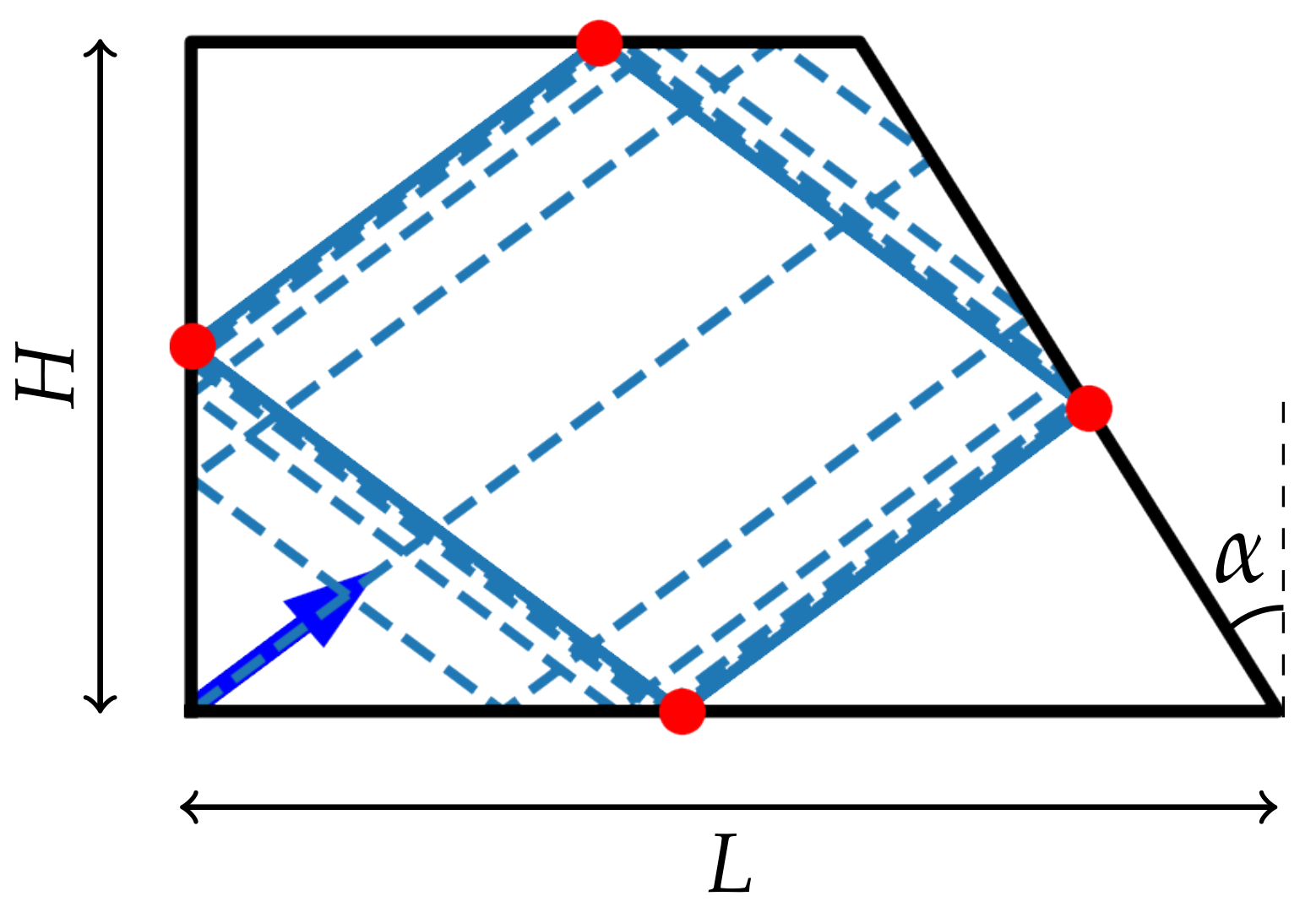
7] and consider the next most simple configuration: the trapezium with one vertical wall and one inclined wall. The sketch of this geometry is given in
Figure 1. The left wall is collinear to gravity and the right wall has slope
.
As initial state we will take a static, stable linear density stratification in which density
consists in a spatio-temporal constant part,
, plus a part decreasing upwards,
. For such a case a displaced particle oscillates with the buoyancy or Brunt-Väisälä frequency:
here
y is the vertical coordinate, directed anti-parallel to gravity acceleration,
g.
The external forcing of the system can be a periodic body force of “tidal” origin as in [
7,
18], or can be produced with a wavemaker at part of the boundary [
19,
20,
21,
22]). Numerous laboratory experiments successfully reproduced the dynamics of the wave attractors with the help of a wavemaker, located at the left (vertical) wall at
and having a half-cosine shape [
8,
9,
10,
23,
24]:
where
, and
denotes the period at which the wavemaker oscillates.
The full boundary-value problem with initial conditions will be presented in
Section 4, numerically solving the incompressible Navier–Stokes equations. In the present and next section we will focus on geometrical properties of internal wave propagation. This is dictated by the dispersion relation for plane internal waves in unbounded fluids with linear stratification. It has a very special form [
17]:
where
is the angle between the phase velocity vector and gravity. A remarkable property of such a dispersion relation is the orthogonality of the group velocity vector to the phase velocity vector (their vertical components pointing in the same direction).
In the case of an ideal fluid, the complete set of parameters characterizing the state of the described system with a uniformly stratified incompressible fluid is:
Following [
7] we can transform coordinates:
after which the number of independent parameters will be reduced to just two. The first transformation translates and compresses the horizontal largest base of the trapezium to the interval [−1,1]. The second transformation scales the vertical coordinate so that the wave beams propagate at the angle
to vertical and horizontal. As a result, we get only two dimensionless parameters:
In
Figure 1 one can see how the attracting limit cycle can be formed when the beam of internal waves originates from the lower left corner as indicated by the blue arrow. The limit trajectory has one reflection from either lateral boundary, and one reflection from either horizontal boundary, hence the name (1,1) attractor.
The wave beam approaches the limit cycle at a rate that can be characterised with the help of the Lyapunov exponent. In [
7] the diagram of Lyapunov exponents over the
parameter plane was given. It can be seen from this diagram, copied below in
Figure 2, that the area of existence of a (1,1) attractor has the form of a triangle. In
Section 3 we show that it can be easily computed analytically and extended for integer
. On the other hand, the shape of the area of existence of a more general (n,m) attractor with n horizontal and
vertical cells can have a more complex shape [
25]. Note that attractors require m to be odd, as for even m a focusing reflection at inclined walls is exactly balanced by a defocusing reflection. In this case a regular global mode (with m cells in the vertical) appears, similar to those in a rectangular domain.
For example in [
25] the shape of (1,3) and (2,3) regular modes is given. In the next section we will give exact expressions for the coordinates of boundary reflections of (n,1) attractors and areas of their existence on a
diagram.
A very peculiar feature of regimes with wave attractors is that in this case a bounded (and simply connected) hydrodynamic system admits the solution in the form of travelling waves [
26]. This is quite unusual since traditionally the solution for such an enclosed geometry is looked for in the form of standing waves. Here, however, inside enclosures, the attractor acts as an ’infinity inside’. It allows the application of a radiation condition, otherwise applied to open domains only. This condition now allows for phase propagation under the constraint that the corresponding energy propagation is towards the attracting limit cycle, and not in opposite direction.
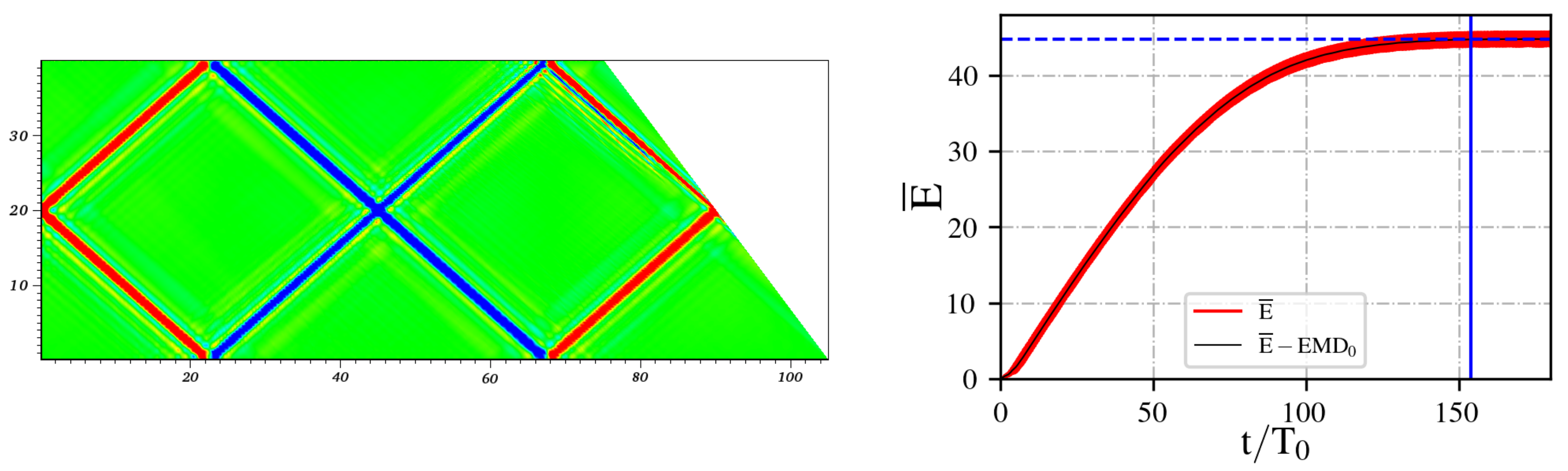
In
Figure 3 one can see the typical field of vertical velocity after a (1,1) attractor has established together with the evolution of the total kinetic energy. The details of numerical simulation will be covered in
Section 4, the parameters correspond to the laboratory experiments with the wavemaker located at the vertical wall as in [
8,
27]. The total kinetic energy
is normalized by the maximum kinetic energy of the wave maker oscillating at amplitude
a in Equation (
1). The exact definition of
corresponds to the one given in [
28].
In the case of standing waves, the kinetic energy would periodically approach zero, just as for a pendulum, but here we observe the accumulation of kinetic energy into travelling waves. An important characteristic of this kind of motion is the time needed to establish the final wave regime. We will refer to this time as the saturation time. In natural or laboratory conditions, the time needed for the system to change from one state to another may be too long compared to other characteristic changes in the system, hence the practical importance of this time interval.
Here we define the saturation time as the time when the difference between the averaged kinetic energy over the next 10 external forcing periods () and the final value of the averaged kinetic energy becomes smaller than 0.001.
3. The Algorithm for Calculation of the Coordinates of an (n,1) Attractor
By coordinates of an (n,m) attractor we mean the coordinates of the points of intersection of the rays with the boundary of the domain.
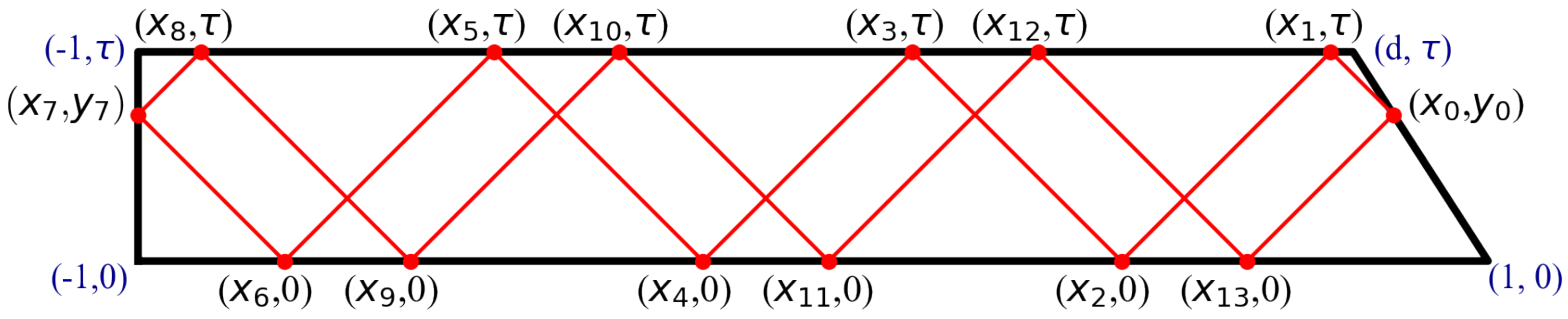
A concise system of notation for the coordinates is presented in
Figure 4. The coordinates of the point at the right wall are denoted
, this point is chosen as the beginning for the wave beam cycle, and an alternative notation for this point is
. The next points are given following the direction of energy propagation: the second point has the coordinates
, the third
and so on. The
-th point will lie on the left wall, so below we use also the alternative notation for this point
.
The coordinates in
Figure 4 are calculated with the help of Formulae (
6) given below.
It seems that the expressions for the exact coordinates of (1,1) attractor first appeared in [
29], but we reproduce here a different approach, which is based on the non-smooth continuations [
30], since such an approach allows generalisations and description of an algorithm for the exact computation of the coordinates of (n,m) attractors.
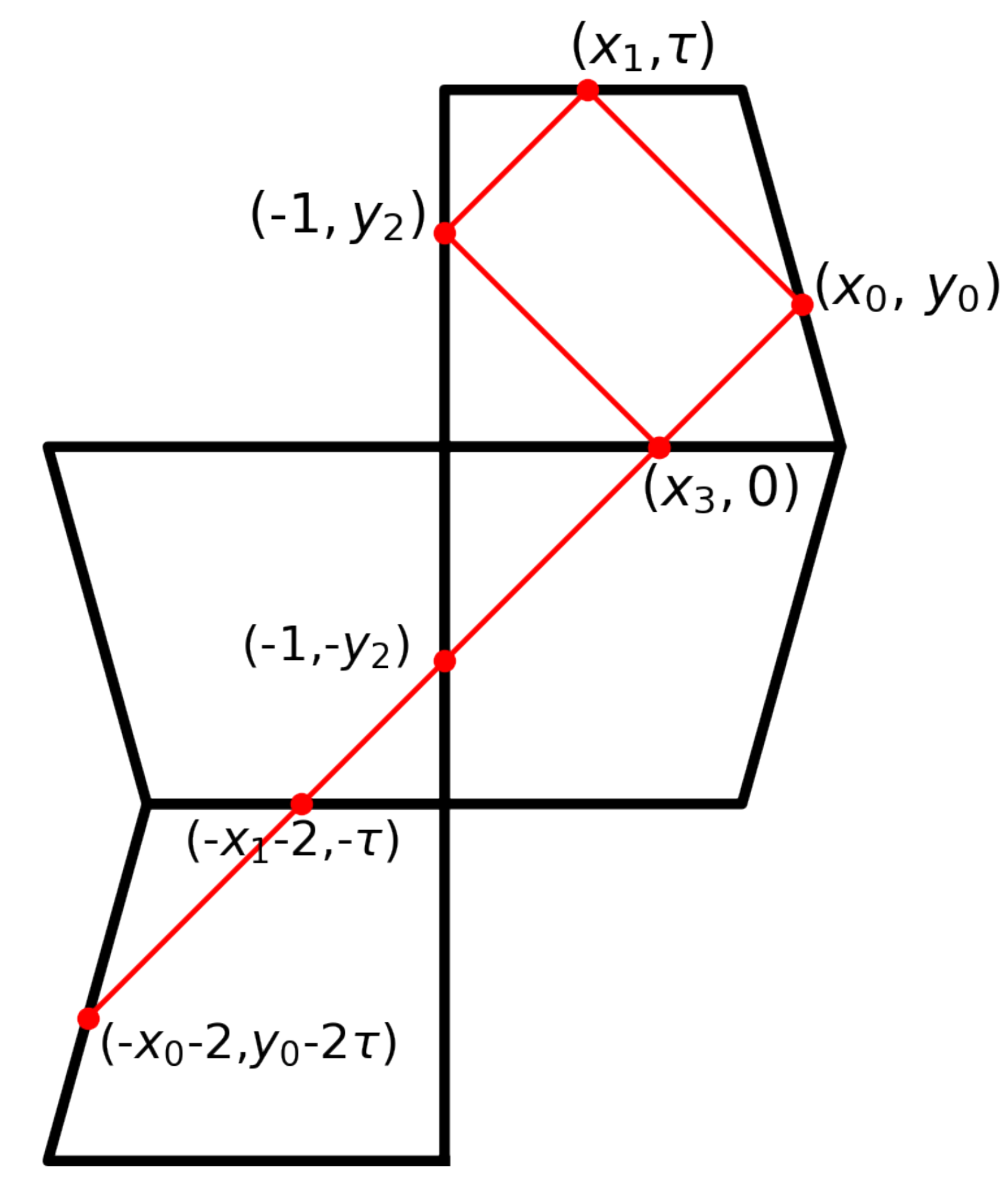
The basic idea of obtaining the exact expression for the coordinates of the (n,1) attractor is the application of the method of non-smooth transformation. We will first demonstrate it on the (1,1) attractor, and next give the general formulas for the (n,1) attractor.
Figure 5 shows the application of this idea. See also a discussion on unfolding in [
25,
31] which is used to find the coordinates of the (1,1) attractor. First, we reflect the trapezium with respect to the left vertical boundary. Next the upper half-plane is reflected with respect to the horizontal lower boundary. After that we emit the ray from some point at the right vertical boundary downwards, and follow its intersections with the reflected trapeziums. It can be easily seen that if we follow the straight line through the reflected trapeziums the fourth point may return again to the right wall. To get the closed loop of rays with one reflection at each wall, in other words to get the (1,1) attractor, the fourth point has to fall onto the initial point at the right wall. Let us write the conditions that all the points belong to the same line:
Finally, we add the condition that (
) lies on the right wall:
The solution of this system of equations reads:
The advantage of such an algorithm as compared to the one described in [
29] is the possibility of its application to a more general (n,1) or even (n,m) cases (for odd
m). For the (n,1) case, the attractor is either symmetric with respect to its central vertical axis in case of even n, or anti-symmetric with respect to its center (the graph remains unchanged after rotation by
about its center) for
n odd. This is why
in the case of even n, and
in the case of odd n. (These symmetries allow to generalize the ray model solutions for a trapezium under consideration to the corresponding symmetrical domains which are shown in
Figure 6 with dashed lines.) Following the same procedure as with the (1,1) attractor we get the expressions for the coordinates of a (n,1) attractor:
Expressions for
in (
6) give the constraints for the area of existence of
attractor, since
,
,
:
These inequalities define triangles in the
plane with three vertices:
The corresponding areas of the existence of (n,1) attractors are plotted in
Figure 2 over the diagram of Lyapunov exponents, which were computed according to a method described in [
7].
Expression for
in (
6) allows to give exact formulae for the Lyapunov exponents
in case of (n,1) attractors. Since the perimeter of the (n,1) attractor is equal to
and the beams after reflections from the slope get closer by the focusing parameter
[
24]:
4. Direct Numerical Simulation
The boundary value problem of the laboratory setup given in
Section 1 can be described with the following system of Navier–Stokes equations in Boussinesq approximation [
8], which consists of momentum equations, equations of transport and diffusion of salt, and continuity equation:
where
is the velocity,
is the difference between the pressure and hydrostatic (unperturbed) pressure,
is the minimal density,
is the mass force which is
in case of internal waves, and Coriolis force in case of a homogeneous rotating fluid.
is the density of salt in the fluid,
—the Schmidt number. On the vertical boundary the horizontal velocity corresponds to the time-derivative of its position given by Equation (
1); on the other boundaries the velocity vanishes. The boundary conditions for salinity is the absence of flux through the boundary, i.e., equality to zero of its normal gradient at all the boundaries. Direct numerical simulation (DNS) was performed with the help of the spectral element approach and open code nek5000 [
32,
33]. We have thoroughly tested and validated this numerical approach in [
8,
9] where the results of numerical simulation were compared with laboratory experiments on internal wave attractors both in laminar and turbulent regimes. Not only qualitative but also quantitative agreement (to about 10% of discrepancy) was shown in three-dimensional simulations.
Figure 7,
Figure 8 and
Figure 9 show the vertical velocity field in the cases of (1,1), (2,1) and (6,1) attractors. For the sake of clarity of these images the viscosity in DNS was decreased by a factor of 100 as compared to the experiments [
8,
23], which corresponds to increasing spatial dimensions. Such a scaling allows to analyse the general structure of (n,1) attractors in viscous fluids, and underlines major differences in its behaviour with (1,1) attractors, which were thoroughly studied in a number of publications. In particular, the saturation time increases almost linearly with the number of reflections (in the present numerical study, the number of reflections is also proportional to the horizontal dimension). For a (1,1) attractor it is 96.1
, for a (2,1) attractor it is 154
, and for a (6,1) attractor-368.6
, where
is the period of external perturbations, the
Figure 10 shows the linear approximation of the saturation times on number of cells, n. In the asymptotic state, a balance is reached between geometric focusing and viscous/diffusive broadening of the beam. The scale at which this state saturates corresponds to a certain group velocity with which the energy propagates around the limit cycle. The length of the attractor divided by that group speed sets the duration time taken by travelling once around the attractor in its saturated state. This time obviously must increase linearly with n. Each additional cell gives an extra time increment equal to the time taken to propagate along the four sides of that cell. However,
Figure 10 also displays an offset: the time needed to get focusing in the first place, namely from the global scale
at which the forcing along the left wall acts, to the small viscous scale—the beam thickness at which the beam saturates.
Figure 10 demonstrates both linear dependence of the saturation time on the number of cells and the offset at
.
5. Conclusions
We derived the exact expressions for the calculation of the coordinates of wave attractors with one reflection from a lateral wall and n reflections from a horizontal wall. The geometry of the tank corresponds to the setup described in [
7]. The areas of existence of (n,1) wave attractors have the shape of a triangle in the
parameter plane and are given with the help of inequalities. The expression for the Lyapunov exponents and their connection to the focusing parameters is given analytically.
Direct numerical simulation of the stratified fluid subject to external forcing at a boundary fully supports the theory and shows that (n,1) attractors can be effective in translating global forcing to travelling waves.
The time of saturation, needed for the wave regime to develop from the state of rest to the final steady wave motion, increases almost linearly with the growth of n.
This paper can be considered as the first part of a three-step analysis of the internal waves mixing and energetics in the case of (n,1) attractors. The second part will be devoted to mixing, and the third will combine ray-tracing, DNS and neural networks for the prediction of the average mixing efficiency.


