Vertical Shear Processes in River Plumes: Instabilities and Turbulent Mixing

Abstract

In this paper, the problem of vertical shear flow instabilities at the base of a river plume and their consequences in terms of turbulent energy production and mixing is addressed. This study was carried out using 2D non-hydrostatic simulations and a linear stability analysis. The initial conditions used in these simulations were similar to those observed in river plumes near estuaries. Unstable stratified sheared flows follow three stages of evolution: (i) the generation of billows induced by vertical shear instabilities, (ii) intensification, and (iii) elongation. The elongation of the generated billows is related to the strain intensity, which depends on the physical setting involved (velocity shear, stratification thickness, and bottom slope). Two vertical shear instabilities were found in our study: the Holmboe and Kelvin–Helmholtz instabilities. The Kelvin–Helmholtz instability has a smaller growth time and longer wavelengths; the Holmboe instability is characterized by a longer growth time and shorter wavelengths. The Kelvin–Helmholtz instability is intensified when the bottom is sloped and for large shears. The Holmboe instability is stronger when the stratification thickness is reduced compared to the shear thickness and when the bottom is sloped. For mixing, the flow can be: (i) pre-turbulent, (ii) quasi-turbulent, or (iii) turbulent. The pre-turbulent flow corresponds to more mass mixing than momentum mixing and to more Eddy Kinetic Energy dissipation than Eddy Available Potential Energy dissipation. Such a flow is encountered over a flat bottom whatever the initial shear is. The quasi-turbulent and turbulent flows are reached when the bottom is sloped and when the stratification thickness is reduced. Using turbulent mixing statistics (mixing coefficients, mixing efficiency, Eddy Kinetic Energy, and Eddy Available Potential Energy dissipation rates), we showed that, despite their slow growth, Holmboe instabilities contribute more efficiently to turbulent mixing than Kelvin–Helmholtz instabilities. Holmboe instabilities are the only source of turbulent mixing when sharp density gradients are observed (small buoyancy thickness experiment). Our simulations highlight the contribution of the Holmboe instability to turbulent mixing.

1. Introduction

Kelvin–Helmholtz (hereafter KH) instability was first proposed by Helmholtz in 1868 [1]. He argued that the assumption of a fluid being free from friction is not true in its interior. Indeed, using an analogy with electricity, he showed that the flow of two neighboring fluids results in surface separation. This surface separation evolves as a discontinuity in the velocity field in the neighboring fluids. The surface discontinuity was considered as a surface of gyration where moments of rotation are generated by frictional processes. Thomson [2] showed that under the action of wind waves, disturbances can be observed below the ocean surface, which evolve into small waves that travel fast and finally cease, except when the disturbing force (the wind) continues to act. These growing waves are manifestations of the Kelvin–Helmholtz instability; they can roll up into vortices with horizontal axes, named “billows”. This instability was studied with a mathematical model that featured two fluid layers with uniform and distinct velocities and densities. This study was then generalized by Taylor [3] and Goldstein and Taylor [4] using an arbitrary vertical velocity profile in a continuously stratified fluid. The flow instability equation was obtained from the linearization of the three-dimensional non-hydrostatic equations. A condition for instability was obtained based on the Richardson number; the minimum Richardson number should be lower than a threshold of 0.25.

The KH instability exists in different geophysical and astrophysical flows. In the Jupiter atmosphere, the interaction between the solar wind and the magnetosphere favors the development of vortices [5,6,7]. These vortices result from a KH instability initiated in the subsolar region and advected by magnetospheric flows to the dusk sector. Magnetic KH instability and its features (vortices) have also been observed at the surface of a fast coronal mass ejecta in the Sun [8]. Unstable flow nonlinearities favor the transport of momentum, plasma, and energy in both large-scale and micro-scale turbulence. In the atmosphere, KH vortices are observed in the upper troposphere and above the tropopause [9,10]. These vortices have diameters larger than 200 m and a characteristic period of 12 min. They are related to maxima in the vertical wind shear.

In the ocean, KH vortices are high-frequency and small-scale features that have been studied in a wide range of flow conditions in stratified shear flows. These vortices result from successive processes: (i) a primary Kelvin–Helmholtz instability, (ii) a vortex merger, and (iii) secondary Kelvin–Helmholtz instabilities. The primary Kelvin–Helmholtz instability is generated at the interface between two neighboring fluids [11,12,13]. These authors used field measurements, numerical simulations, and laboratory experiments to observe such instabilities. Primary KH instabilities were observed in a tilted tank (in the spanwise direction), with fluid in the two layers being unequally distant from the shear interface [11]. The author indicates that the primary KH instability is delayed in the asymmetric case compared with the symmetric configuration. KH vortices, which are a result of a primary KH instability, were identified in the seasonal thermocline off San Diego, California, in 1988 [12]. These authors found, using turbulent velocity measurements, that these vortices have a horizontal scale of about 3.5 m. Primary instability waves have been observed in a stratified flow in the Knight inlet [13]. These authors conducted laboratory experiments with two reservoirs containing fluids of (slightly) different densities, flowing over a 2D sill in a rectangular channel. They deduced that the shear interface fluctuations are due to internal seiche and to primary Kelvin–Helmholtz instabilities. The KH billows (resulting from primary KH instabilities) at the interface of a stratified shear flow can then undergo a merging process [14,15].

The merging process of a pair of Gaussian vortices has been studied in different stratification conditions. In a weak stratification, vortex mergers proceed in several stages: a diffusive/axisymmetrization phase, a convective/deformation phase, a convective/entrainment phase, and a final diffusive/axisymmetrization phase [14]. In these stages, the interaction between vorticity gradients and the rate of strain is central. Brandt and Nomura suggest that their effects on stratification are controlled by the ratio between the growth of cores (billows cores) and viscous effects (quantified by the Reynolds number). In contrast, in intermediate to high stratification, vortex mergers are not always possible as strong baroclinic vorticity prevents them and induces a low diffusivity; the drift of the vorticity centroid can be observed [15]. Billow mergers or drifts are followed by the growth of higher-order harmonics associated with a secondary Kelvin–Helmholtz instability [13,16]. A secondary KH instability arises in the vicinity of KH billows. When the density interface is sharp enough, another secondary instability appears: the Holmboe instability [17,18,19]. The unstable shear flow, when the density stratification length scale is much smaller than the shear length scale, undergoes a Kelvin–Helmholtz instability with a steady vortex formed at the middle of the interface; this is accompanied by a Holmboe instability with waves traveling along the interfacial boundary [19]. In general, different regions can be defined in an unstable shear flows: (i) a region with neutral gravity waves, (ii) a region where two Holmboe modes propagate in the opposite direction, (iii) a region where KH instability exists, and (iv) a region with singular neutral modes [18]. After the onset of vertical shear instabilities (KH and Holmboe), a transition to turbulence occurs [11,12,13,20]. KH instability favors entrainment between the neighboring layers and therefore mixing [13]. The turbulent patches thus formed are characterized by a spectral slope of $-2$; they are limited by mixing occurence in the sloping direction [11,12]. In laminar and turbulent flows, the KH vortices can develop and pre-existing turbulence may affect the onset of Kelvin–Helmholtz instability [20].

In river plumes, KH instability can be observed in estuaries and the near-field region (near the river mouth). This instability can be generated by many physical effects: winds, river discharge, and tides. Tedford et al. [21] observed a one-sided instability (KH instability) in the Frazer River estuary using an echo sounder. They compared field measurements with the Taylor–Goldstein equation modes. They suggested that the interaction between river discharge and tides produces KH instability above or below the density interface. In their study, mixing and turbulence result from strong tidal velocities near the bed and from shear instabilities. These instabilities have also been studied along the North Passage of the Yangtze river estuary using a high-resolution nonhydrostatic model [22]. The authors found that the interaction between freshwater discharge and tides tempers the duration and length scale of the KH vortices. Moreover, in their study KH instability induces a high mixing efficiency with maximum mixing rates of $5\times {10}^{-6}$ J m${}^{-2}$ s${}^{-1}$. These turbulent fine structures influence the behavior of tidal plumes [23]. Iwanaka and Isobe [23] conducted field surveys near a river mouth and used a nonhydrostatic model; they showed that small horizontal scale features (<100 m) can be observed in the tidal plume. They related these small eddies to inertial and Kelvin–Helmholtz instabilities and indicated that such instabilities act like friction, which prevents tidal plumes from expanding offshore. In different oceanic regions, the KH instability induces mixing and turbulent processes [24]. In numerous studies, the vertical diffusivity, reached when KH vortices are observed, lies between ${10}^{-4}$ and ${10}^{-3}$ m${}^2$ s${}^{-1}$ [25,26]. In highly stratified river plumes, the size of KH billows (Ozmidov scale) is O(10 cm) [26]. Thus, these small scale eddies can be difficult to observe. In most river plumes, the KH billows occupy less than 10% of the interfacial volume but achieve significant mixing [26].

In the present work, a 2D nonhydrostatic model is used to perform idealized numerical simulations of stratified shear flows characteristic of river plumes. The following issues will be addressed:

• What is the evolution of a sheared river plume base under different flow parameters?
• Which type of vertical shear instabilities can affect the plume base and under which flow conditions?
• What are the effects of the vertical shear instabilities on vertical turbulent mixing?

The paper will be organized as follows: The model equations, configuration, simulations, and methods will be described in Section 2; the 2D structure and life cycle of the plume and its interface will be presented in Section 3.1; the vertical shear instabilities affecting it will be described in Section 3.2; and the turbulent mixing and the efficiency that those instabilities induce will be given in Section 3.3. The main results will be discussed in Section 4 and conclusions will be provided in Section 5.

2. Materials and Methods

2.1. Model Configuration

The simulations were performed using the Fluid2d numerical model. Fluid2d is a versatile Python–Fortran CFD (Computational Fluid Dynamics) model provided by http://pagesperso.univ-brest.fr/~roullet/fluid2d/ (acccessed on 20 December 2021). Fluid2d is used to simulate a large range of 2D flows. It is defined on a C-Arakawa grid, where tracers (buoyancy, vorticity) are discretized at model cell centers. Velocity components and stream functions are discretized at cell edges and cell corners, respectively. The time discretization scheme is explicit. In our study, velocity and density equations in the (x-z) plane, under the non-hydrostatic (NH) approximation, are used. In this approximation, an incompressible and stratified fluid with no Coriolis effect is considered. No explicit viscosity, nor explicit diffusivity are used here. The NH Boussinesq equations are written as:

$${\partial }_{x}u+{\partial }_{z}w=0$$

(1)

$$\frac{D\mathbf{u}}{Dt}=-\Delta p+b\mathbf{k}$$

(2)

$$\frac{Db}{Dt}=0$$

(3)

where $\mathbf{u}=u\mathbf{i}+w\mathbf{k}$ ($\mathbf{i}$ and $\mathbf{k}$ are the horizontal and vertical unit vectors, respectively) is the velocity vector, p is the pressure scaled by a mean density ${\rho }_0$, b is the buoyancy, and $\frac{D}{Dt}={\partial }_t+\mathbf{u}.$ Δ is the material derivative.

The first NH equation indicates that the velocity is derived from a streamfunction with $w={\partial }_x\psi$ and $u=-{\partial }_z\psi$. Therefore, the vorticity is deduced as $\omega ={\partial }_{x}w-{\partial }_{z}u={\Delta }^2\psi$. The latter lead to the vorticity and buoyancy equations summarized below:

$${\partial }_t\omega +J(\psi ,\omega )={\partial }_{x}b$$

(4)

$${\partial }_{t}b+J(\psi ,b)=-N^2{\partial }_x\psi$$

(5)

$${\partial }_{xx}^2\psi +{\partial }_{zz}^2\psi =\omega$$

(6)

where $\omega$ is the vorticity, b is the buoyancy field, J is the Jacobian operator, $N^2$ is the Brunt–Vaisala frequency, and $\psi$ is the streamfunction.

The model uses a third order Runge–Kutta (Stably Strongly Preserving scheme) as a time stepping scheme. The advection scheme is a fifth-order upwind for both tracers and momentum that has the advantage of built-in dissipation. Neither explicit viscosity nor diffusivity are used here. The grid size in pixel units is 512 × 2048 in the (z-x) plane and the time step is 0.01 s. The horizontal and vertical extents of the model grid are 40 m and 10 m, respectively. A periodic boundary condition is applied in the x direction and a free-slip boundary is applied in the vertical direction. The model runs for 4 modeled minutes with outputs every quarter of a second. The model has no external forcing nor Coriolis effect. The Coriolis effect could be added but in our case it is not mandatory, since the simulation time is far below the inertial period.

2.2. Model Experiments

Here, a description of the different experiments performed in this study is provided. Starting from the reference case, sensitivity experiments were carried out, which involved different flow parameters or topographic ridges. In all the experiments, the initial conditions were a shear-stratified flow; the background velocity and buoyancy vertical profiles were:

$$B=N_0^2{h}_{b}tanh\left(\frac{z-z_0}{h_b}\right)$$

(7)

$$U=-S_0{h}_{s}tanh\left(\frac{z-z_0}{h_s}\right)$$

(8)

where $h_s$ is the thickness of the shear layer and $h_b$ is the thickness of the stratified layer (Figure 1). The thickness is assumed to be identical for both of these fields ($h_b=h_s$), except in experiment 3, where the stratification thickness is much smaller than the shear layer thickness ($h_b=\frac{h_s}{1000}$). The thickness retained in these experiments is 2 m, which corresponds to an average value of the freshwater thickness in river plumes in previous studies [27,28,29]. $z_0$ is the vertical location of the interface, which is taken here as the mid-depth.

$N_0^2$ is the Brunt–Vaisala frequency, which is computed as:

$$N_0^2=\frac{g\Delta \rho }{{\rho }_{0}H}$$

(9)

where H is the total water depth (here 10 m), g is the acceleration gravity, ${\rho }_0$ is the mean density (here 1025 kg·m${}^{-3}$), $\Delta \rho$ is the density difference between two layers (taken here as 15 kg·m${}^{-3}$ [26]) which leads to a Brunt–Vaisala frequency of 0.01 s${}^{-2}$. This parameter is fixed for all the experiments shown here.

A total of 4 experiments were carried out in this study. Between these experiments, we also varied $S_0$, the square root of the vertical shear $S^2={\left({\partial }_{z}u\right)}^2+{\left({\partial }_{z}w\right)}^2$. Most experiments used a flat bottom, except the last experiment, where topographic ridges were introduced. The bottom shape $z_b$ of the last experiment can be written as:

$$\begin{array}{cc}{z}_b(x)=1.5\times (1-cos\left(\pi \frac{x-5}{5}\right)),& \mathrm{if}5\le x\le 35\\ 0,& \mathrm{otherwise}\end{array}$$

(10)

White noise is added to the initial vorticity to trigger the instability. The initial minimum Richardson number is below the critical threshold (0.25), which ensures the generation of vertical shear instabilities.

Table 1. Simulation parameters.

Experiments	Initial Shear (s${}^{-2}$)	Initial Stratification (s${}^{-2}$)	Minimum Richardson Number	Interface	Bottom	Boundaries
Reference	0.25	0.01	0.04	plane ($h_b=h_s$)	flat	Periodic in x + Rigid in z
Exp 2	0.5	0.01	0.02	plane ($h_b=h_s$)	flat	Periodic in x + Rigid in z
Exp 3	0.25	0.01	0.04	plane ($h_b=\frac{h_s}{1000}$)	flat	Periodic in x + Rigid in z
Exp 4	0.25	0.01	0.04	plane ($h_b=h_s$)	sloping	Periodic in x + Rigid in z

summarizes the simulations performed in this study.

2.3. Diagnostics for Stratified Sheared Flows Structure and Dynamics

Since we wish to examine the life cycle of the billows at the interface of the stratified sheared flow, several diagnostics will be defined. Each billow will be characterized by: (i) its centroid position ($x_c,z_c$), (ii) its radius, and (iii) its aspect ratio. The geometrical moments of vorticity are defined as in Dritschel [30] and we write:

$$J_{mn}=\int {\int }_D{x}^m{z}^n\omega (x,z)dxdz$$

(11)

The centroid of each billow is defined as:

$$x_c=\frac{J_{10}}{J_{00}},z_c=\frac{J_{01}}{J_{00}}$$

(12)

The billow semi-major axis a and semi-minor axis b are defined as in Le Dizès and Verga [31], and we write:

$$a^2={\displaystyle \frac{J_{20}co{s}^2\left(\varphi \right)-J_{11}sin\left(2\varphi \right)+J_{02}si{n}^2\left(\varphi \right)}{J_{00}}},b^2={\displaystyle \frac{J_{02}co{s}^2\left(\varphi \right)-J_{11}sin\left(2\varphi \right)+J_{20}si{n}^2\left(\varphi \right)}{J_{00}}}$$

(13)

where the rotation angle and the radius of each billow are expressed as:

$$\varphi =\frac{1}{2}arctan\left(\frac{2J_{11}}{J_{20}-J_{02}}\right),r=\frac{\sqrt{\pi ab}}{\pi }$$

(14)

The average radius of the identified billows for each experiment is quantified. Then, the moving average (over 30 s) of the billows’ aspect ratio $\frac{b}{a}$ is represented.

The spatial distribution of the Okubo–Weiss parameter [32,33] is computed as:

$$OW=s_n^2+s_s^2-{\omega }^2$$

(15)

where $\omega$ is the vorticity, $s_n=-2{\partial }_{z}w$ is the normal strain, and $s_s={\partial }_{x}w+{\partial }_{z}u$ is the tangential strain.

The Okubo–Weiss parameter identifies regions where the vorticity dominates (OW < 0) and regions where the strain dominates (OW > 0).

Then, the surface average of the strain intensity $s^2=s_n^2+s_s^2$, and the strain direction ${\alpha }_{strain}=arctan\left(\frac{s_n}{s_s}\right)$ in regions where OW is positive are computed.

The moving average (over 30 s) of these strain diagnostics is compared to the aspect ratio.

2.4. Diagnostics for Instabilities

A decomposition of the flow is performed. The mean flow is the background state (initial conditions) and perturbations are obtained for the velocity components (u and w) and the buoyancy field as:

$$b^{\prime }(x,z,t)=b(x,z,t)-b(x,z,t=0)=b(x,z,t)-B(x,z)$$

(16)

$$u^{\prime }(x,z,t)=u(x,z,t)-u(x,z,t=0)=u(x,z,t)-U(x,z)$$

(17)

$$w^{\prime }(x,z,t)=w(x,z,t)-w(x,z,t=0)=w(x,z,t)$$

(18)

A measure of the turbulence intensity in the stratified shear flow is the eddy kinetic energy, which is expressed as:

$$EKE\left(t\right)=\frac{1}{2L{H}_c}{\int }_0^L{\int }_0^{H_c}(u^{\prime }{(x,z,t)}^2+w^{\prime }{(x,z,t)}^2)dxdz$$

(19)

where L is the horizontal length of the domain and $H_c$ is the critical layer, as defined in Appendix A.

Then, a linear stability analysis is performed using non-hydrostatic (NH) approximation. A linear analysis of the stability is performed to identify the nature of the instability, its growth, its phase speed, and its critical layer depth. The EKE of each identified instability is also computed. Full details about this linear stability analysis are given in Appendix A.

2.5. Diagnostics for Turbulent Mixing

The turbulent mixing is quantified using by the vertical eddy viscosity $K_m$ and the vertical diffusivity $K_b$ [34]:

$$K_m=-\frac{1}{L{H}_c}{\int }_0^L{\int }_0^{H_c}\frac{u^{\prime }{w}^{\prime }}{{\partial }_{z}U}dxdz$$

(20)

$$K_b=-\frac{1}{L{H}_c}{\int }_0^L{\int }_0^{H_c}\frac{w^{\prime }{b}^{\prime }}{{\partial }_{z}B}dxdz$$

(21)

Then, the vertical EKE dissipation $ϵ$ [35] and the vertical buoyancy dissipation ${ϵ}_b$ are evaluated as:

$$ϵ=-\frac{1}{L{H}_c}{\int }_0^L{\int }_0^{H_c}\frac{u^{\prime }{w}^{\prime }}{{\partial }_{z}U}({\left({\partial }_z{u}^{\prime }\right)}^2+{\left({\partial }_z{w}^{\prime }\right)}^2)dxdz$$

(22)

$${ϵ}_b=-\frac{1}{L{H}_c}{\int }_0^L{\int }_0^{H_c}\frac{w^{\prime }{b}^{\prime }}{{\partial }_{z}B}{\left({\partial }_z{b}^{\prime }\right)}^{2}dxdz$$

(23)

The turbulent Prandtl number is then deduced from the vertical diffusivity and the vertical eddy viscosity as $P_r=\frac{K_m}{K_b}$.

The irreversible mixing efficiency ${\Gamma }_i=\frac{\Gamma }{1+\Gamma }$ is evaluated [36], where $\Gamma$ is the mixing efficiency deduced from $K_b=\Gamma \frac{ϵ}{{\partial }_{z}B}$ [35]. This irreversible mixing efficiency will be computed for each vertical shear instability (Holmboe and Kelvin–Helmholtz) using modal decompositions of the vertical EKE dissipation and the vertical diffusivity that we write as:

$$\widetilde{K_b}=-\frac{1}{L{H}_c}{\int }_0^L{\int }_0^{H_c}\frac{Re\left(\tilde{w}{\tilde{b}}^{\ast }\right)}{{\partial }_{z}B}dxdz$$

(24)

$$\widetilde{ϵ}=-\frac{1}{L{H}_c}{\int }_0^L{\int }_0^{H_c}\frac{Re\left(\tilde{u}{\tilde{w}}^{\ast }\right)}{{\partial }_{z}U}({\partial }_z\tilde{u}{\partial }_z{\tilde{u}}^{\ast }+{\partial }_z\tilde{w}{\partial }_z{\tilde{w}}^{\ast })dxdz$$

(25)

The mixing is considered efficient if ${\Gamma }_i$ is larger than 0.2 [37].

3. Results

3.1. Structure and Dynamics of Stratified Sheared Flows

Here, we present and analyze the time evolution of the stratified–sheared interface. The interface corresponds to a river plume base. The centroid of vorticity is computed with different parameters (average radius of billows, ratio of centroid distance over the average radius, magnitude of the strain and its direction, and Okubo–Weiss parameter) to describe the dynamical processes governing the evolution of the coherent vortices formed at the plume base. Several sensitivity experiments are carried to understand the dynamics of the antisymmetric sheared flow in different settings.

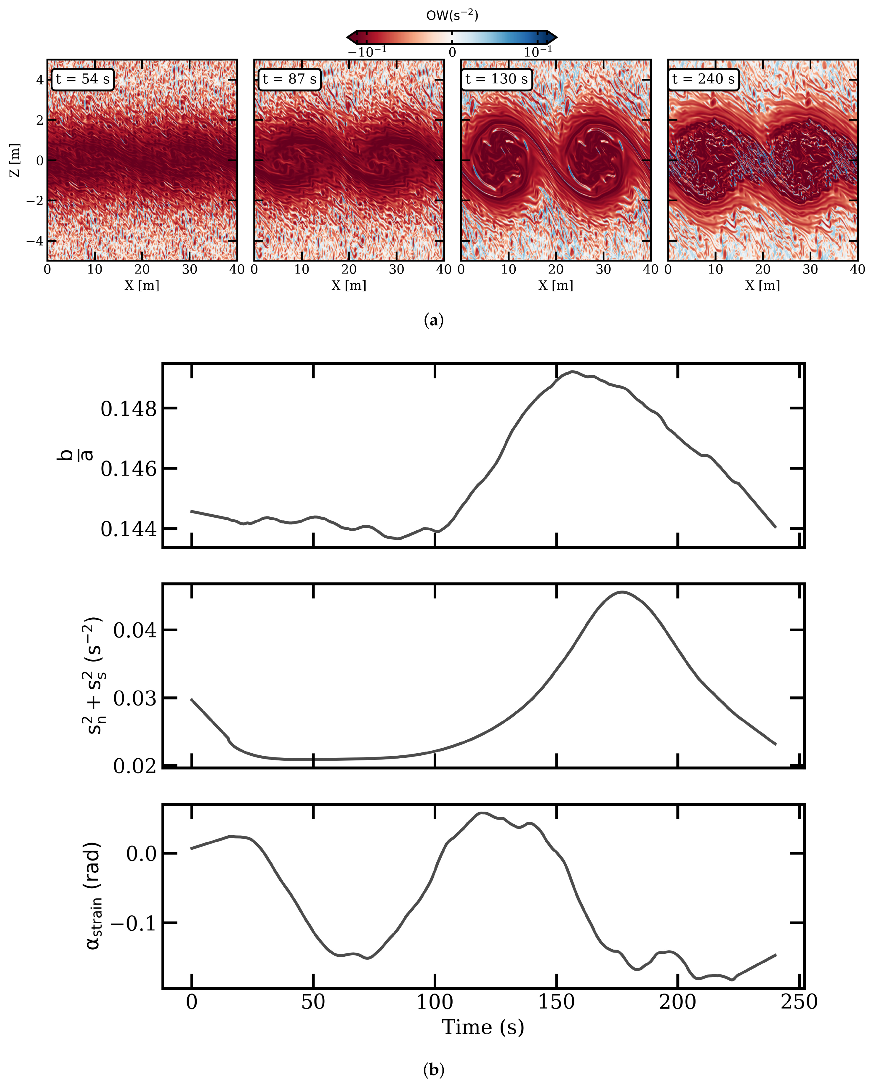
3.1.1. Reference Configuration

Figure 2 shows the time evolution of the buoyancy and vorticity fields at different stages of the reference simulation. During the first period of this simulation (for 8 < t ≤ 54 s), the anti-symmetric shear causes the buoyant plume interface to deform and crests and troughs are generated. The advection of water parcels across the interface produces vorticity that evolves from a noisy field at the beginning to a wavy stripe engulfing the sheared interface (see Equation (4)). Then (for 87 ≤ t ≤ 130 s), the crest of perturbation moves upward; this forms a flow constriction in the upper layer. The flow constriction accelerates the flow in the upper layer and a roll-up of the shear layer is observed, which generates small eddies (billows). These billows are two small cyclonic eddies, with an average radius of 3.8 m, and their roll-ups favor fluid entrainment between the two layers. Finally (at $t\sim 240$ s), the two cyclonic billows elongate; this elongation triggers the development of small-scale filaments at their rims and in their cores.

The billows have a strong vorticity, which competes with the fluid strain. This competition can be evaluated with the Okubo–Weiss (OW) parameter (Figure 3a). The vorticity dominates (OW < 0) in the sheared layer during the generation, intensification, and elongation of the billows. Meanwhile, the strain dominance (OW > 0) is patchy during the period of generation of the billows (at $t\sim 54$ and 87 s). Intense strain is found at the edges of small filaments located in the upper layer (2 m below the surface) and the lower layer (2 m above the bottom). During this period (for $t<100$ s), the strain is mostly tangential (${\alpha }_{strain}\sim -0.1$ rad) and remains constant (its intensity ∼0.02 s${}^{-2}$), as shown in Figure 3b. This indicates that, during this period, the vorticity favors the generation of the billows and thus the influence of the strain is not prominent.

Then, the billows roll up and are intensified (at $t\sim 130$ s). The strain remains dominant at the same locations as in the previous periods. It is prominent in small-scale features in the core of the billows and in the thin tilted interface formed between the billow cores: the braid. During the period of intensification of the billows (at $t>100$ s), the strain intensity increases sharply and reaches a maximum (∼0.045 s${}^{-2}$) at $t\sim 150$ s. The strain is mostly tangential during this period, as its direction is nearly horizontal. This tangential strain induces an elongation of both billows in the horizontal direction, since their aspect ratio increases sharply up to values of ∼0.15.

The billows reach their full extension during the last period (at $t\sim 240$ s). The spatial distribution of the strain dominance is localized in small filaments in the core of the billows and between them. Since the elongation of each billow reaches half of the horizontal domain length, each billow is constrained by the other; then, their aspect ratio decreases notably (at $t>150$ s) and therefore the tangential strain (${\alpha }_{strain}\sim -0.1$ rad) slackens.

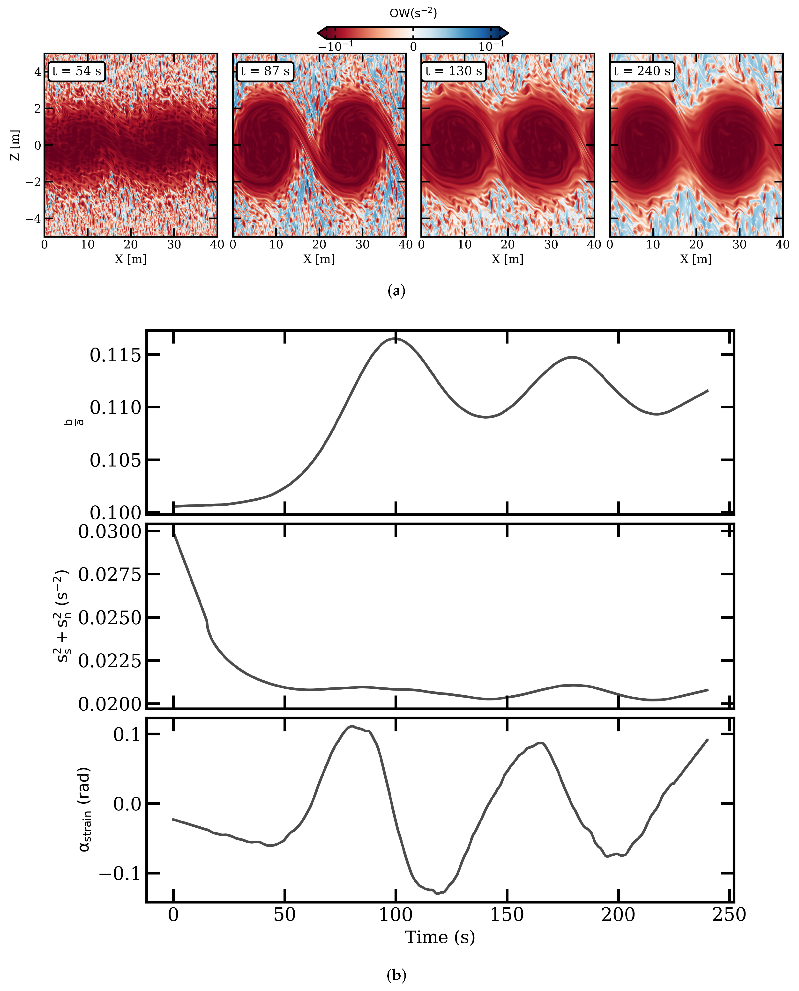
3.1.2. Sensitivity to the Vertical Shear (Exp2)

In this simulation, the (initial) vertical shear is twice that of the reference experiment. Figure 4 shows the time evolution of the vorticity and buoyancy fields. During the first period (for $8<t\le 54$ s), the sharp interface evolves quickly and by the end of this period buoyant crests appear. The vorticity field is noisy and intense and, at the end, turbulent structures are observed in the sheared interface. Then (for $87\le t\le 130$ s), the perturbed interface evolves to form two intense cyclonic billows which begin to roll; due to the fluid acceleration in the upper layer and the induced tangential strain, they extend in the horizontal direction. These two billows have a radius of ∼3.8 m. Finally (at $t\sim 240$ s), these two cyclonic billows elongate in the tangential direction and their extent reaches half of the domain length. Filaments and strong vorticity are observed in their core and at their rims.

In this experiment, during the generation of vortices ($t\sim 54$ s) the Okubo–Weiss parameter is weakly positive locally in the top and bottom layers around small filaments and negative in the sheared layer (Figure 5a). Prior to this period (at $t\le 54$ s), the tangential strain (${\alpha }_{strain}$∼ 0 rad) intensity remains weak (Figure 5b). This indicates that, during this period, the flow develops intense vorticity that will contribute to the two billow cores.

Then (at $t\sim 87$ s), the vortices are formed and roll up. The strain dominance increases in the upper and lower layers, in small strips in the inner core of the billows, and along the braid. This induces a sharp increase in the intensity of the tangential strain (${\alpha }_{strain}$∼ 0.1 rad), reaching values up to 0.05 s${}^{-2}$ at $t\sim 100$ s. The sharp increase in the tangential strain induces a deformation of both billows, as indicated by the sharp growth in their aspect ratio (a maximum ∼0.1525).

Lastly (t∼ 130 and 240 s), the vortices are elongated and intensified. Their elongation and intensification induce straining in their cores and along the interface separating the billows. The vorticity is still dominant in the sheared layer. During this period (at $t>100$ s), the billows’ aspect ratio is neither decreasing nor increasing. This is due to the generation of strong vorticity complemented by a tangential elongation of both vortices. The two elongated billows cover the length of the domain and therefore limit the growth of the strain. The intensity of the strain decreases during this period. The strain remains tangential, as its direction is ∼0 rad.

Thus, the billow radii in this simulation are identical to those of the reference experiment. Despite this similarity, the vortices are formed earlier here and the growth of their aspect ratio here is larger than in the reference experiment. This is mainly due to the intensity of the tangential strain, which reaches 0.05 s${}^{-2}$ compared to 0.04 s${}^{-2}$ in the reference configuration. The stronger shear favors the earlier generation of billows.

3.1.3. Sensitivity to the Thickness of the Interface (Exp3)

In this simulation, the stratification thickness is much smaller than the shear thickness (see Table 1). Figure 6 shows snapshots of the spatial distribution of buoyancy and vorticity fields. During the first period (for $8<t\le 54$ s), small perturbations form at the thin buoyant interface. By the end of this period, the small perturbations evolve as two crests propagating in the opposite direction of the two troughs. Then (for $87\le t\le 130$ s), the perturbations evolve as two cyclonic billows that elongate in the direction of the sheared flow. Finally ($t\sim 240$ s), the billows reach their full horizontal extent and filaments develop in their cores. The average radius of these billows is ∼3.8 m.

During the linear stage of the instability (at $t\sim 54$ s), the vorticity dominates the strain almost everywhere in the domain, except in local strips in the top and bottom layers (Figure 7a). The billows are not definitely formed yet and their aspect ratio remains weakly varying (∼0.145), as shown in Figure 7b. The billows aspect ratio varies with a decreasing strain intensity during this period. The strain is tangential (its direction is ∼0 rad).

Then (at $t\sim 87$ s), the sheared layer rolls up and two distinct billows are formed. The billows induce intense vorticity in the sheared layer and along the braid (OW < 0). The billows also lead to an intensified strain in the upper and bottom layers. The aspect ratio of the two billows grows and reaches values of (∼0.11). Despite the growth in their aspect ratio, the intensity of the strain varies weakly (∼0.02 s${}^{-2}$) with a tangential direction (∼0.1 rad).

Finally (at $t\sim 130$ and 240 s), the billows intensify and elongate. During this period, the vorticity is still dominant in the sheared layer. Meanwhile, the strain dominance is noticeable above and below the sheared layer. The billow aspect ratio increases (at $t>150$ s) and weakly intensifies the tangential strain (∼0.02 s${}^{-2}$).

Thus, in comparison to the reference simulation, the average radius of the billows remains the same. Despite this similarity, their aspect ratio is larger and the tangential strain is less dominant. The reduced stratification thickness helps in the earlier growth of billows. Meanwhile, it induces less strain in the core of the billows and along the braid.

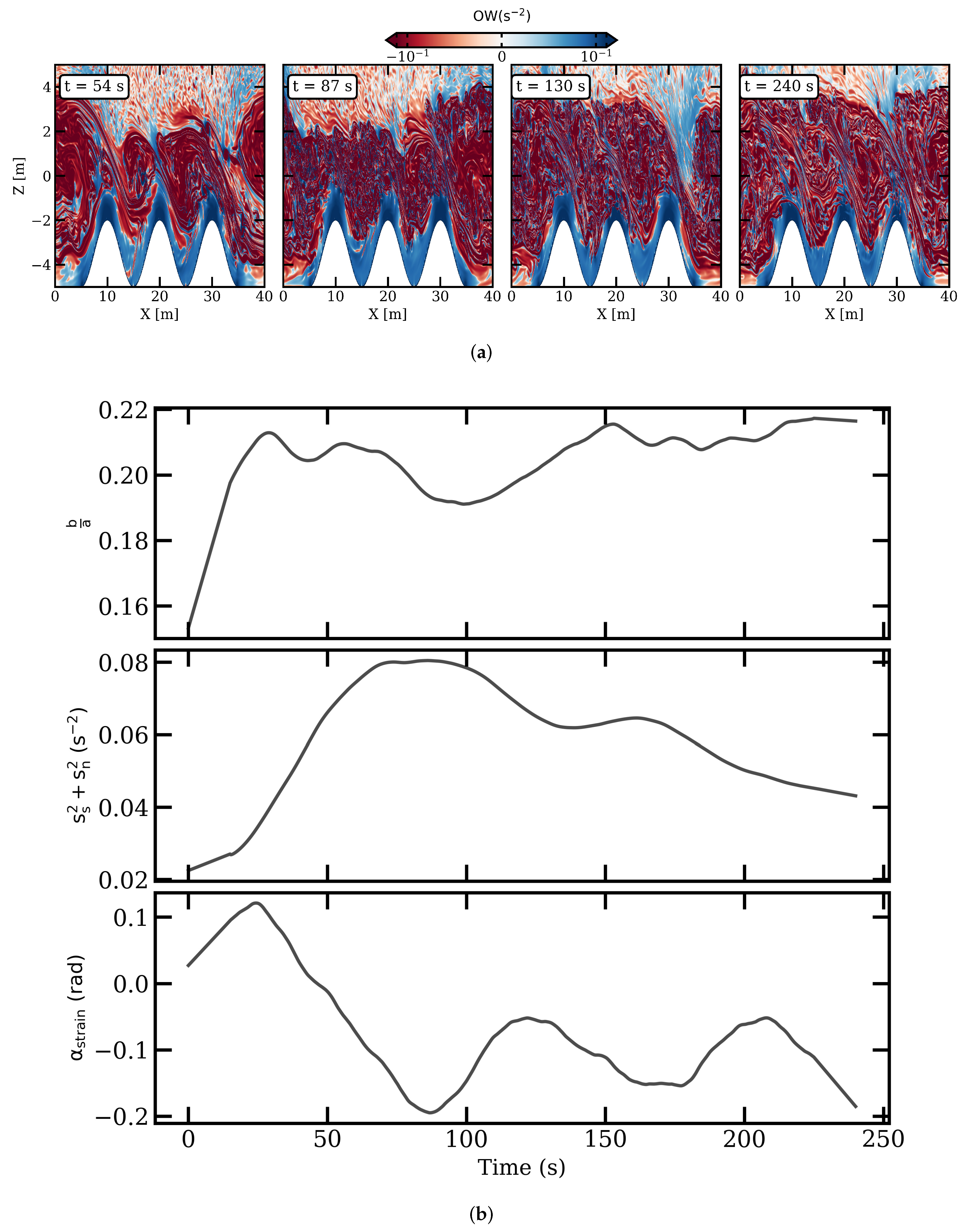
3.1.4. Sensitivity to Topographic Ridges (Exp4)

Figure 8 shows the time evolution of the (plane) buoyant interface above topographic ridges. Firstly (for $8\le t\le 54$ s), the antisymmetric sheared flow and its interaction with ridges cause the deformation of the plume base. This deformation yields three distinct cyclonic billows of different sizes (average radius ∼ 3 m). These three billows mutually interact, which alters their respective shapes. These billows also interact with the topographic ridges, which favors their stretching. Then (for $87\le t\le 240$ s), the sheared flow evolves in different chaotic vortices and anticyclonic filaments are generated at their edges due to their mutual interactions and their stretching above the ridges.

Next, the spatial distribution of the Okubo–Weiss parameter is evaluated (Figure 9a). First (at $t\sim 54$ s), the vorticity dominates in the sheared layer, albeit with some straining in the core of the billows. During this period ($t\le 54$ s), the intensity of the strain increases sharply (∼0.01 s${}^{-2}$), as shown in Figure 9b. The growth in the strain exhibits an elongation of the billows in the tangential direction (aspect ratio ∼ 0.2). After this period ($t>54$ s), the elongation of the eddies nor increases nor decreases due to: (i) the mutual interactions between the billows; (ii) the billows’ vertical extent, which constricts the regions where the strain dominates, causing the latter to weaken; and (iii) the continuous interaction between the billows and the topographic ridges.

Thus, in comparison with the reference configuration, the interaction between topographic ridges and the anti-symmetric shear flow favors the development of three distinct cyclonic billows. The average size of the billows is small compared with the reference configuration due to their mutual interaction and their stretching above the ridges. The tangential strain is also noticeable above the ridges, which increases its intensity compared with the reference configuration.

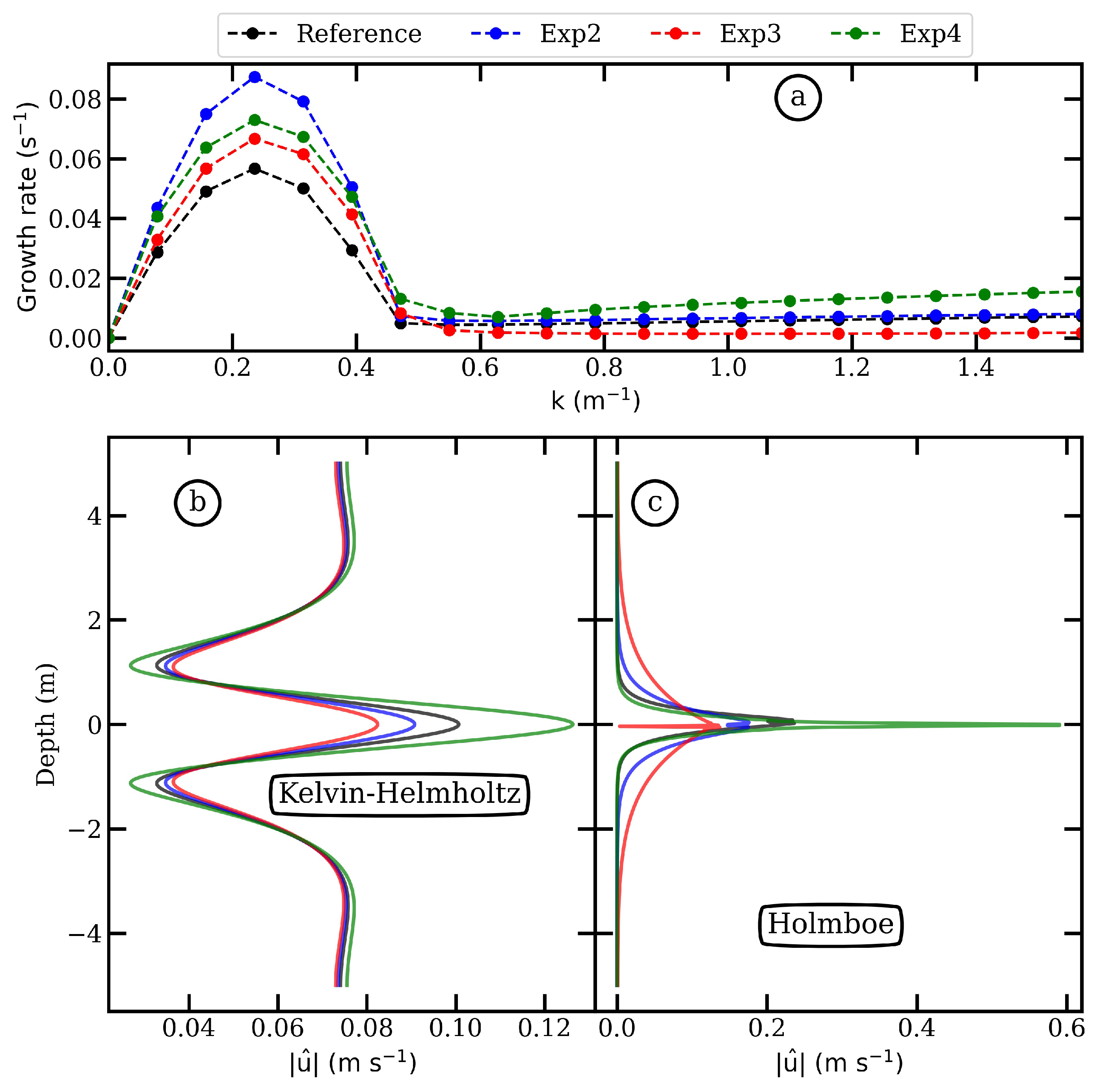
3.2. Modal Analysis and Instability Growth

In this section, the most unstable modes of the stratified–sheared river plume base are evaluated. Those unstable modes are categorized as Holmboe and Kelvin–Helmholtz instabilities, as described in Section 2.4. Their growth, their vertical structure, and the time evolution of their turbulent energies are computed. The sensitivity of these instabilities to the various parameters is explored.

3.2.1. Reference Configuration

Two vertical shear instabilities are investigated here, the Kelvin–Helmholtz and the Holmboe instabilities. The vertical shear instabilities exist since the necessary condition for their development (a Richardson number smaller than 0.25) is already satisfied in the initial conditions. The Kelvin–Helmholtz instability is characterized by a large growth rate and zero phase velocity. The Holmboe instability has a nonzero phase velocity and smaller growth rates.

The linear stability theory is used to investigate these instabilities (Figure 10a). This analysis predicts that Kelvin–Helmholtz instability occurs for large wavelengths ($k\sim 0.23$ m${}^{-1}$, $\lambda =\frac{2\pi }{k}$∼ 27 m). The Holmboe instability occurs for smaller wavelengths ($k\sim 5.4$ m${}^{-1}$, $\lambda$∼ 1 m). The identification of Holmboe instability is investigated using the bifurcation theory, as shown in Figure A1 and explained in Appendix B.

The most unstable mode for the Kelvin–Helmholtz instability has a growth time scale ∼17.6 s. The Holmboe instability unstable mode develops slowly with a growth period of ∼88.4 s. The Holmboe waves have a phase speed of 2.4 cm s${}^{-1}$.

Next, the vertical structure of the magnitude of the streamwise velocity for the Kelvin–Helmholtz and Holmboe instabilities is explored (Figure 10b,c). The Kelvin–Helmholtz mode has a constant velocity at the surface and near the bottom. In this mode, the streamwise velocity is maximal (∼10 cm s${}^{-1}$) at the sheared interface or at the critical layer (around mid-depth) and surrounded with minima (∼3.3 cm s${}^{-1}$) at the upper and lower density interfaces. These minima have the same amplitude and are symmetric with respect to the critical layer depth. The Holmboe mode is characterized by a local minimum (∼22.3 cm s${}^{-1}$), as observed at the critical layer. This local minimum is found in a thin layer (of a few cm) surrounded by two secondary lobes. The upper lobe flows slightly faster than the lower lobe.

Now, the horizontally and vertically (from the surface to the critical layer) averaged Eddy Kinetic Energy (EKE) for the total, Kelvin–Helmholtz, and Holmboe perturbations are evaluated (Figure 11a). Early time ($0<t\le 50$ s) is associated with a slight increase in the total EKE, which characterizes the onset of the instability. Then (at $50<t\le 150$ s), a sharp increase in the total and KH EKE is observed, indicating that the instability fully develops into two distinct cyclonic billows and the initiation of their elongations. Then, a decrease in the total and KH EKE is observed, since the billows are well developed and dissipation can occur.

The KH mode turbulent energy represents an important fraction of the total EKE (∼10%). The Holmboe instability, characterized by smaller wavelengths, develops when the KH instability slackens or relaxes. The EKE associated with Holmboe instability is much smaller (${10}^4$ smaller) than the KH EKE. This indicates that the KH instability is the dominant nonlinear process in the reference simulation.

3.2.2. Sensitivity to the Vertical Shear (Exp2)

In this case, the KH instability develops for larger wavelengths ∼27 m and a growth time of ∼11.4 s (Figure 10a). Meanwhile, the Holmboe instability develops for smaller wavelengths ∼2 m ($k\sim 2.9$ m${}^{-1}$) and a slower growth time of 112 s. The Holmboe instability induces turbulent waves that travel slowly with a phase speed of ∼0.7 cm s${}^{-1}$.

Now, the vertical structure of the streamwise velocity for each instability is analyzed (Figure 10b,c). For the Kelvin–Helmholtz instability, the streamwise velocity is uniform in the top and bottom 2 m. This velocity diminishes in the upper density interface with a local minimum of 3.5 cm s${}^{-1}$. In the shear layer (between $-2$ and 2 m), the flow is faster with a maximum of 9 cm s${}^{-1}$. It is again slower at the lower-density interface. This shows that the KH instability is intensified in the shear layer while it slackens at both density interfaces. Meanwhile, the vertical structure of the Holmboe mode has a minimum (∼15 cm s${}^{-1}$) at the critical layer (depth ∼ 5 m) surrounded by two lobes. The lower lobe travels faster than the upper lobe. The Holmboe instability results, therefore, in two waves traveling at different speeds around the critical layer.

Finally, the time evolution of the EKE for the total perturbations and the KH and Holmboe decompositions is examined (Figure 11b). The total and KH EKE start to increase when the generation of the KH instability starts (at $t>40$ s). Then, these turbulent energies reach a maximum at around 90 s once the billows are fully formed. After this peak, the total and KH EKE increase again during two distinct periods (for $125<t\le 150$ s and between 175 and 200 s). These peaks correspond to the elongation of the billows and their intensification. Their intensification leads to the development of small-scale features in their cores, which may also increase the EKE. The Holmboe energy increases during periods when the total and KH energies weaken. The KH instability represents the dominant process in this experiment (it is stronger than the Holmboe instability by ${10}^3$).

Thus, compared to the reference configuration, the stronger shear (i) speeds up the growth of the KH instability, (ii) retards the growth of the Holmboe instability, (iii) increases the wavelength of the Holmboe instability, (iv) enhances the energetic contribution of Holmboe instabilities by an order of magnitude, and (v) diminishes the propagation of Holmboe waves with a lower layer (near the critical layer) traveling faster than the upper layer.

3.2.3. Sensitivity to the Thickness of the Interface (Exp3)

When the thickness of the buoyant layer is small compared with the shear thickness, the KH and Holmboe instabilities co-exist. The KH instability is characterized by larger wavelength ($\lambda$∼ 27 m) and a faster growth time ∼15 s (Figure 10a). The Holmboe instability grows slowly (∼663 s) with a smaller wavelength of ∼5 m. The Holmboe waves propagate with a phase speed of ∼2 cm s${}^{-1}$.

Now, the vertical structure of the Holmboe and KH instabilities is evaluated (Figure 10b,c). The streamwise velocity increases in the shear layer has a maximum of 8 cm s${}^{-1}$ and is slower at the upper and lower shear interfaces (∼4 cm s${}^{-1}$). The streamwise velocity for the Holmboe mode is minimal (∼0.05 cm s${}^{-1}$) around the critical layer. Two layers are observed around this critical layer propagating at different speeds. The upper layer moves slightly faster than the lower layer.

To quantify the turbulent activity, the time evolution of the EKE for the total, KH, and Holmboe perturbations is plotted (Figure 11c). The total and KH EKE increase after the onset of the vertical shear instabilities (at $t>50$ s). They reach a maximum at $t\sim 100$ s once the cyclonic billows are generated. Then, they increase again after 150 s to reach a second maximum at $t\sim 180$ s. These second maxima correspond to the elongation and intensification of the billows. Holmboe EKE increases during periods of relaxation of both the total and KH EKE. Holmboe instability may exist in this case, but its contribution is weak (${10}^2$ times smaller than the KH energy).

Thus, compared with the reference simulation, a small buoyancy thickness: (i) speeds up the generation of the KH instability, (ii) slows down the development of the Holmboe instability, (iii) increases the spatial wavelength of the Holmboe instability, and (iv) slightly diminishes the propagation speed of the Holmboe waves.

3.2.4. Sensitivity to Topographic Ridges (Exp4)

In the presence of topographic ridges, the KH and Holmboe instabilities co-exist. The KH instability grows quickly in time (at ∼14 s) and develops spatially with a wavelength of ∼27 m (Figure 10a). The Holmboe instability grows with a shorter wavelength of ∼1 m. Its growth period is ∼46 s. The Holmboe instability waves propagate slowly, with a phase speed of ∼0.5 cm s${}^{-1}$.

Then, the vertical structure of the KH and Holmboe instabilities in terms of the streamwise velocity magnitude is evaluated (Figure 10b,c). The streamwise velocity of the Kelvin Helmholtz mode of instability increases in the shear layer (∼12.5 cm s${}^{-1}$) and slackens at the edges of this layer. The Holmboe instability mode has a streamwise velocity, which weakens at the critical layer and strengthens above and below this layer with the same speed (∼60 cm s${}^{-1}$).

Finally, the total, KH, and Holmboe EKE during the simulated period are analyzed (Figure 11d). The total EKE grows rapidly and reaches a maximum at $t\sim 50$. Similarly, the KH EKE increases rapidly due to the fast generation of billows. Then ($t>100$ s), the total EKE decreases due to frictional processes induced by the interaction between the billows and the topographic ridges. The latter is also observed for the KH EKE. Meanwhile, the Holmboe EKE grows during periods of relaxation/decrease in the KH instability but with a smaller contribution (${10}^3$ smaller).

Thus, in comparison to the reference simulation, the topographic ridges (i) strengthen the growth of KH and Holmboe instabilities due to the interaction of the sheared flow with topographic ridges which accelerate the fluid, (ii) dissipate the KH instability through frictional processes, and (iii) slow down the Holmboe-induced waves and alters their wavelengths.

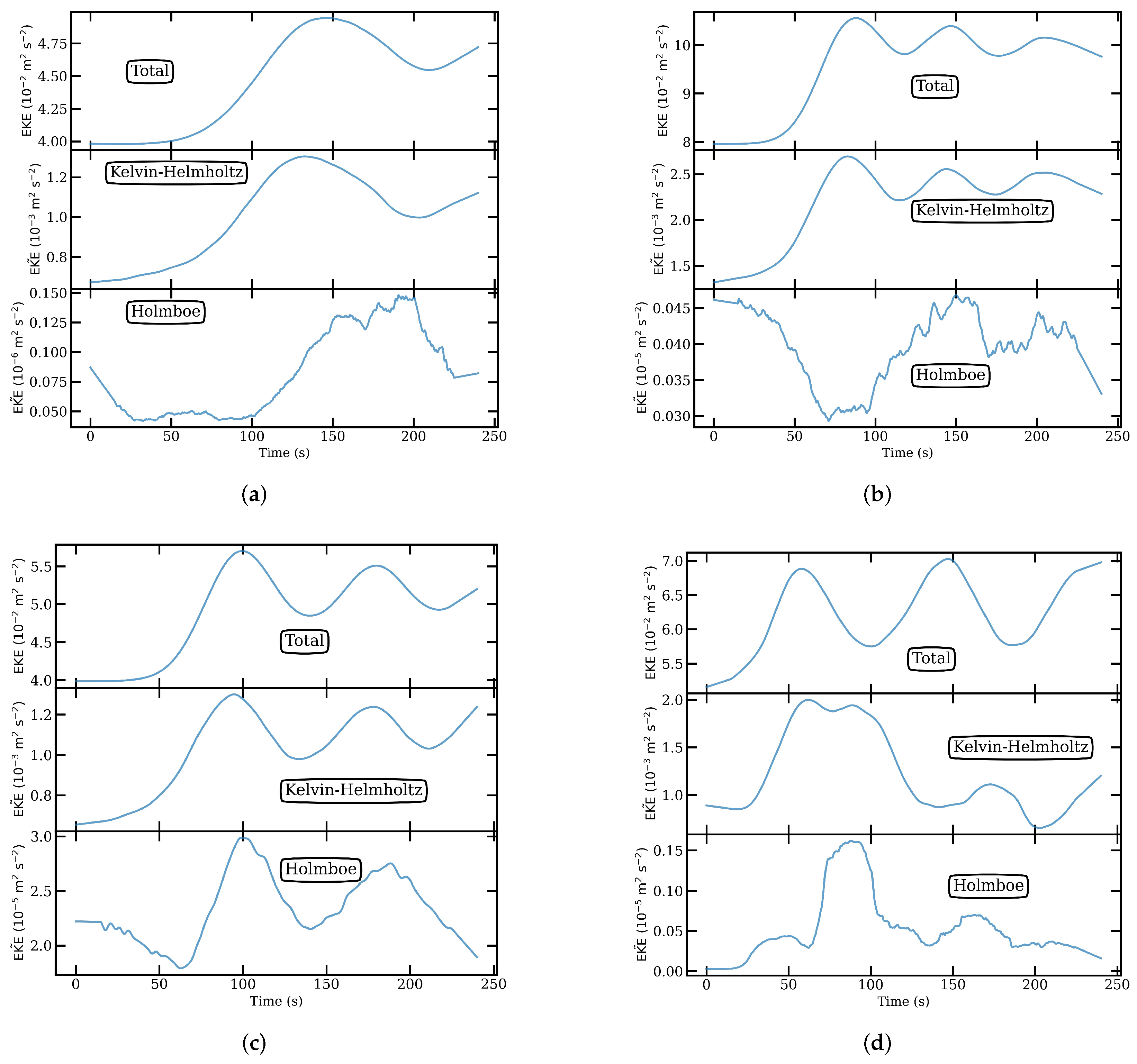
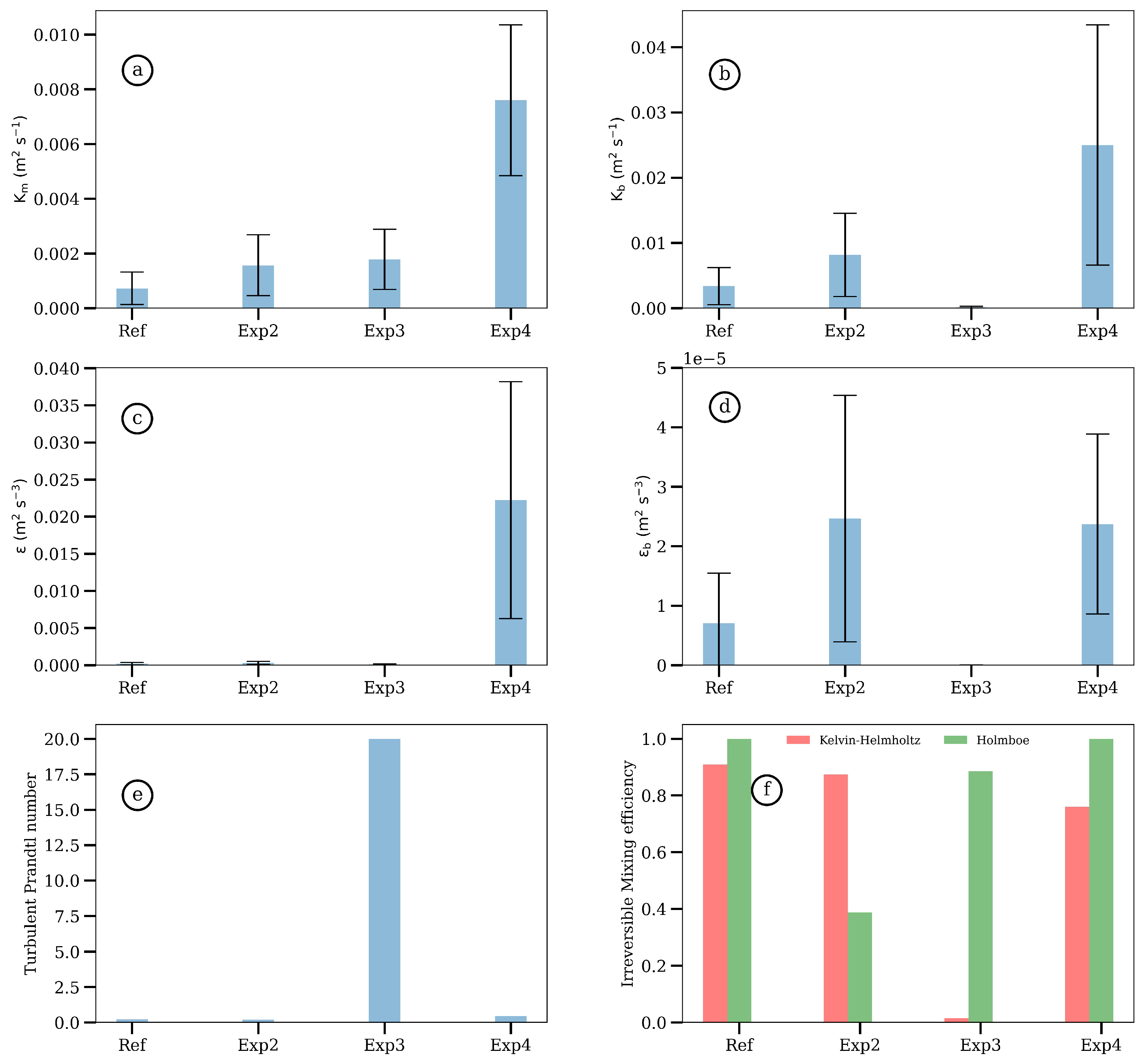
3.3. Turbulent Mixing

In this section, the turbulent mixing is characterized by: (i) the EKE production, (ii) the buoyancy and EKE dissipate rates, and (iii) the mixing statistics.

3.3.1. Reference Configuration

First, the time evolution of the mass and momentum mixing coefficients and their dissipation rates are evaluated (Figure 12a). After the onset of instability (at $t>50$ s), the turbulent mixing of mass and momentum sharply increase until it reaches a maximum at $t\sim 120$ s. This maximum corresponds to the generation of billows which favor fluid entrainment and therefore mixing between the upper and lower layers. Since turbulent energy is produced via mixing, an energy sink is necessary. Dissipative processes (of EKE and EAPE/buoyancy) contribute to this sink. The EKE and buoyancy dissipation rates reach a maximum (at $t\sim 150$ s) when the sources of EKE weaken.

Once the billows are formed, they elongate and intensify (for $150<t\le 175$ s). Their elongation and intensification strengthens the water recirculation in their cores and thus the mixing of mass and momentum increases. During this period, the dissipation rates of EKE and of buoyancy increase.

Finally (for $t>175$ s), the production of EKE by mass and momentum mixing decreases. This is also accompanied by smaller dissipation rates of buoyancy and EKE. This is due to the full elongation of vortices, which induce less turbulence; therefore, the production and dissipation of turbulent energy drop.

To quantify the turbulent mixing, the mass and momentum mixing coefficients, the buoyancy, and the EKE vertical dissipation rates, the turbulent Prandtl number and the irreversible mixing efficiency are plotted (Figure 13). The turbulent Prandtl number is ∼0.2, which is far less than unity (Figure 13e). This indicates that the flow is in a pre-turbulent phase. This state is due to large mass mixing $K_b$∼$3.4\times {10}^{-3}$ m${}^2$ s${}^{-1}$ compared with the momentum mixing $K_m$∼ $7.2\times {10}^{-4}$ m${}^2$ s${}^{-1}$ (Figure 13a,b). The pre-turbulent flow and its mixing coefficients are largely due to the high EKE dissipation $ϵ$∼$2\times {10}^{-4}$ m${}^2$ s${}^{-1}$ compared with weak EAPE dissipation ${ϵ}_b$∼$7\times {10}^{-6}$ m${}^2$ s${}^{-1}$ (Figure 13c,d). The pre-turbulent flow is influenced by the KH and Holmboe instabilities. They influence the turbulent mixing, as can be quantified with the irreversible mixing efficiency. Here, the Holmboe instability is more efficient (${\Gamma }_i$∼ 1 > 0.2) in mixing the mass and momentum than the Kelvin–Helmholtz instability (${\Gamma }_i$∼ 0.9 > 0.2), as shown in Figure 13f.

3.3.2. Sensitivity to the Vertical Shear (Exp2)

The enhanced shear favors the early growth of the mass and momentum mixing due to the rapid generation of instabilities (Figure 12b).

The momentum mixing increases (at $t>50$ s) once the shear layer deforms. It reaches a maximum early (at $t\sim 60$ s) of ∼$4\times {10}^{-3}$ m${}^2$ s${}^{-1}$. The dissipation of EKE reaches a maximum (at $t\sim 60$ s) of ∼$5\times {10}^{-4}$ m${}^2$ s${}^{-3}$. After this period (for $t>60$ s), the momentum mixing decreases. Mass mixing shows variations similar to those of momentum mixing, though an order of magnitude larger. Meanwhile, the buoyancy dissipation increases sharply, with a maximum ∼$5\times {10}^{-5}$ m${}^2$ s${}^{-3}$ occurring at $t\sim 100$ s during periods when mass mixing relaxes.

In this experiment, the flow is in a pre-turbulent phase, since the turbulent Prandtl number is ∼0.2 (Figure 13e); momentum mixing ∼$1.6\times {10}^{-3}$ m${}^2$ s${}^{-1}$ dominates over mass mixing ∼$1.6\times {10}^{-4}$ m${}^2$ s${}^{-1}$ (Figure 13a,b). This pre-turbulent flow also corresponds to stronger EKE dissipation ($3\times {10}^{-4}$ m${}^2$ s${}^{-3}$) than buoyancy dissipation ($2.5\times {10}^{-5}$ m${}^2$ s${}^{-3}$) (Figure 13c,d). Turbulent mixing is influenced by the two instabilities, as measured by their mixing efficiencies. The Kelvin–Helmholtz instability contributes more to the mixing (${\Gamma }_i$∼ 0.9 > 0.2) than the Holmboe instability does (${\Gamma }_i$∼ 0.4 > 0.2) (Figure 13f).

Thus, in comparison with the reference configuration, the enhanced shear (i) speeds up the mixing of the mass and momentum, (ii) does not change the nature of the flow (pre-turbulent), (iii) strengthens the momentum mixing and the induced EKE dissipation rates, (iv) weakens the mass mixing and strengthens the EAPE dissipation rates, and (v) intensifies the mixing efficiency induced by the Kelvin–Helmholtz instability and decreases the mixing efficiency induced by the Holmboe instability.

3.3.3. Sensitivity to the Thickness of the Interface (Exp3)

When the stratification thickness is reduced compared to the shear thickness, the momentum mixing increases sharply (at $t>50$ s). It reaches a maximum $4\times {10}^{-3}$ m${}^2$ s${}^{-1}$ at $t\sim 75$ s. The production of EKE is balanced by a growth of EKE dissipation, reaching values of ∼$2.5\times {10}^{-4}$ m${}^2$ s${}^{-3}$. Once the billows are generated ($75<t\le 150$ s), momentum mixing and its induced dissipation decrease. Then (for $t>150$ s), both the sink and the shear production of turbulent energy increase again due to the elongation of the billows, inducing a strong recirculation and as well as favoring mixing and dissipation.

Mass mixing shapes the EKE production in the same way as momentum mixing, with a maximum of ∼$4.5\times {10}^{-4}$ m${}^2$ s${}^{-1}$ at $t\sim 75$ s. Meanwhile, the sink of EAPE through buoyancy increases during periods when the mass mixing relaxes or decreases. Buoyancy dissipation is not important in this case (∼${10}^{-12}$ m${}^2$ s${}^{-3}$); momentum dissipation is thereafter the sole turbulent energy sink.

The flow is in a turbulent phase as $P_r$∼ 10 (Figure 13e). The turbulent flow induces more momentum mixing ∼$3\times {10}^{-3}$ m${}^2$ s${}^{-1}$ than mass mixing ∼$2\times {10}^{-4}$ m${}^2$ s${}^{-1}$ (Figure 13a,b). The sink of turbulent energy is higher for the momentum ∼${10}^{-4}$ m${}^2$ s${}^{-3}$ than for the buoyancy ∼${10}^{-12}$ m${}^2$ s${}^{-3}$ (Figure 13c,d). The Holmboe instability contributes efficiently to the turbulent mixing, since ${\Gamma }_i$∼ 0.6 > 0.2. Meanwhile, the KH instability is not efficient at ${\Gamma }_i$∼ 0.01 < 0.2 (Figure 13f).

Thus, in comparison to the reference configuration, the reduced stratification thickness (i) increases the momentum mixing and decreases the mass mixing, (ii) shapes the flow in a turbulent phase, and (iii) relates the mixing efficiency to the Holmboe instability.

3.3.4. Sensitivity to Topographic Ridges (Exp4)

Figure 12d shows the time evolution of the mass and momentum mixing coefficients, the EKE, and the buoyancy dissipation rates. During the onset of the instability (for $t<100$ s), the momentum mixing and EKE dissipation decrease due to the rapid generation of the billows and their interaction with topographic ridges, which favor frictional processes. Then (at $t>100$ s), the billows are fully developed and engulf almost the entire vertical extent of the domain. The latter induces a strong momentum mixing, reaching ∼${10}^{-2}$ m${}^2$ s${}^{-1}$ with an EKE dissipation rate ∼5$\times {10}^{-2}$ m${}^2$ s${}^{-3}$. The interaction between the topographic ridges and the shear flow induces mixing and EKE dissipation through intense convection and/or bottom frictional processes.

Mass mixing varies as momentum mixing does and reaches values ∼2.5$\times {10}^{-2}$ m${}^2$ s${}^{-1}$. This is related to the vorticity and buoyancy torques in the vorticity transport equation. The EAPE/buoyancy dissipation varies as the mass mixing (∼2.5$\times {10}^{-5}$ m${}^2$ s${}^{-3}$), except during the onset of the instability ($t<100$ s). The strong dissipation of buoyancy is likely due to the interaction between the flow and the bottom during this early period.

In this experiment, the flow is pre-turbulent as $P_r$∼ 0.45 (Figure 13e). The latter is explained by higher mass mixing ∼2.5$\times {10}^{-2}$ m${}^2$ s${}^{-3}$ than momentum mixing ∼7.6$\times {10}^{-3}$ m${}^2$ s${}^{-1}$ (Figure 13a,b). The sink of turbulent energy is higher for momentum ∼2.2$\times {10}^{-3}$ m${}^2$ s${}^{-3}$ than for buoyancy ∼2.4$\times {10}^{-5}$ m${}^2$ s${}^{-3}$ (Figure 13c,d). Both the KH and Holmboe instabilities are efficient (${\Gamma }_i$ > 0.2) in mixing the fluid; the Holmboe instability contributes more (${\Gamma }_i$ ∼ 1.1) to the turbulent mixing than the KH instability does (${\Gamma }_i$ ∼ 0.8) (Figure 13f).

Thus, in comparison with the reference configuration, the interaction between the sheared flow and topographic ridges (i) strengthens the momentum and mass turbulent mixing; (ii) slightly increases the turbulence in the flow, despite the pre-turbulent phase persisting; (iii) favors EKE and EAPE/buoyancy dissipations; and (iv) slightly increases the mixing efficiency of the Holmboe instabilities and decreases the mixing efficiency of the KH instabilities.

4. Discussion

4.1. The Structure and Dynamics of Stratified Sheared Flows

In this paper, the structure and dynamics of stratified sheared flows via 2D non-hydrostatic numerical simulations are studied. In these simulations, the flow evolution in various physical configurations is analyzed.

Firstly, the stratified sheared interface evolves in time from a wavy strip to billows. Sensitivity experiments are carried and compared to a reference simulation. In the flat-bottom cases, the generated cyclonic billows have similar sizes. These sizes are constrained by the interactions, the initial conditions, and the horizontal length of the domain. An enhanced shear and a small buoyant interface trigger an earlier growth of these vortices. The recirculation inside their cores is intensified when the initial shear is increased; this recirculation is weakened when the buoyant interface is thin (compared with the shear layer thickness). This recirculation favors the entrainment between the upper and bottom layers. We also noted that topographic ridges favor the generation of smaller cyclonic billows with anticyclonic filaments at their edges. In this latter case, the antisymmetric shear flow induces noticeable turbulence in the domain.

Secondly, the spatial distribution of the Okubo–Weiss parameter for the different experiments is examined. This tool has been used to identify mesoscale eddies in previous studies [38,39,40,41]. In our experiments, the vorticity dominates in the shear layer when the bottom is flat. The billows are generated in the stratified sheared layer. Over topographic ridges, vorticity is also generated due to frictional processes and fluid acceleration. In this case, the vorticity dominates mostly in the whole domain once strong turbulence is generated.

Thirdly, the spatial distribution and, in particular, the predominance of the strain field are explored. The flow is shown to be strained above and below the sheared layer when the bottom is flat. This is due to the constriction of the flow in these layers, resulting in high-/low-pressure regions. In these cases, the strain is also generated in the cores of the billows and along the braid. The latter is due to the flow recirculation, which may induce local straining. In these experiments, the enhanced shear intensifies the strain in the upper and bottom layers and in the cores of billows due to increased fluid acceleration and recirculation. When the buoyant interface is thin compared to the sheared interface, the straining becomes stronger in the upper and lower layers but weakens inside the billows. This is due to the increased area above and below the buoyant interface, which results in greater pressure forces and therefore in higher strain. Meanwhile, when the bottom is wavy, the strain dominates locally at the edges of the small billows and filaments and above the ridges. This is due to the interaction between the wavy bottom and the antisymmetric flow; this interaction creates more turbulence later in the simulation.

Lastly, the strain is shown to be tangential when the bottom is flat, since only streamwise velocity is considered initially. The tangential strain is found to be correlated with the horizontal elongation of the billows. The tangential strain and the induced billow elongation are intensified when the shear increases, and even more so when the buoyant interface is thin. Such findings can be explained by the tangential force exerted by the enhanced shear on the billows causing their deformation in a parallel direction to the flow (this tangential force is amplified by the increased area when the buoyant interface is thin). This has also been observed for the case of topographic ridges; tangential strain deforms these billows due to the local fluid acceleration induced by friction (above the ridges) and the background shear (top layer).

The generated billows have an average aspect ratio below $\frac{1}{3}$; such an extreme aspect ratio may lead to their splitting in the absence of background strain and shear [42]. However, in our experiments the billows do not split due to their mutual interactions and to the presence of a shear flow. This small aspect ratio is related to the elongation/strain of the billows. In particular, a single billow deforms into an elliptical vortex with filaments at its rim in the presence of background shear [43]. Nevertheless, overall the vorticity dominates the strain in the experiments with billows. This has also been observed in other studies of Kelvin–Helmholtz billows [44].

4.2. Development and Role of KH and Holmboe Instabilities

The vertical shear instabilities in stratified sheared flows are analyzed via linear stability analysis based on 2D non-hydrostatic equations.

Firstly, two vertical shear instabilities are identified: Kelvin–Helmholtz and Holmboe, in our flow configuration. The Kelvin–Helmholtz instability is characterized as the most unstable mode by the linear analysis. The Kelvin Helmholtz instability has a wavelength ∼12 times the shear thickness in the studied cases. The KH wavelength is typically an order of magnitude larger than the shear layer thickness as shown in Smyth and Moum [24]. The wavelengths may also be constrained by the domain geometry and the initial conditions. Vertically, the KH instability has a larger magnitude in the shear layer with a maximum reached at the critical layer (plume base). The Kelvin–Helmholtz instability reaches its maximum amplitude within a time range between 11 and 18 s. Compared to the reference simulation, this instability grows faster and intensifies (in terms of EKE): (i) when the shear increases, (ii) when the shear flow interacts with topographic ridges and also (iii) for a small buoyancy interface thickness.

Secondly, the Holmboe instability is characterized by smaller wavelengths (between 1 and 5 m) and a longer growth time (between 40 and 663 s). The smallest wavelength (∼1 m) and the shortest growth time (∼40–80 s) are found for the reference and wavy bottom experiments. Meanwhile, the enhanced shear slows down the growth of the Holmboe instability (∼112 s), and its wavelength is larger (∼5 m). The small buoyancy thickness induces a Holmboe instability with the slowest growth time (∼663 s) and with a wavelength ∼2 m. The difference between the Kelvin–Helmholtz and Holmboe instabilities is that the first is stationary (zero phase speed) and the second is propagating (non-zero phase speed). The Holmboe instability is characterized by two counter-propagating waves (lobes) above and below the plume base. At the plume base, the magnitude of the streamwise velocity is minimal (and maximal above and below) for the Holmboe instability; it is maximal for the Kelvin–Helmholtz instability. In terms of turbulent energy, the Holmboe instability is intensified during periods of relaxation/decrease in the Kelvin Helmholtz instability but with a smaller impact. Indeed, the KH EKE represents an important fraction (∼$10\%$) of the total turbulent energy. Holmboe instability amplification occurs for a sharp buoyancy interface (small buoyancy thickness) and in the presence of a wavy bottom.

Thus, we showed the existence of the primary Kelvin–Helmholtz and Holmboe instabilities in the studied experiments. We showed that a wavy bottom and small buoyancy thickness lead to the intensification of the Holmboe instability. The Holmboe instability has a smaller wavelength and a larger growth time compared with the Kelvin–Helmholtz instability, as shown in Alexakis [18]. Vertically, the Kelvin–Helmholtz instability has a larger influence in the sheared layer with a maximum at the base of the plume. This result is similar to what has been observed at the base of a surface mixed layer when a stratified flow interacts with Ekman-induced currents [24]. The interaction between downwelling favorable winds and the Gironde river plume favors the development of the Kelvin–Helmholtz instability [29,45]. This instability has also been observed and simulated using a 3D NH numerical model in the Yangtze river estuary due to the interaction between tidal flood and high water slack. Kelvin–Helmholtz instability has also been observed and analyzed using the Taylor Goldstein equation in the Frazer river estuary. The authors found that during ebb tide and high discharge events, the wavelength of such instability is ∼24 m, which is similar to the value found in our simulations. Meanwhile, the Holmboe instability is characterized by two counter-propagating waves (nonzero phase speed) within the critical layer (plume base). It also grows slowly compared to the KH instability and with shorter wavelengths. The latter findings have been indicated in previous studies [17,18,46,47]. Carpenter et al. [48] used in situ observations and linear analysis stability theory, indicating the coexistence of the KH and Holmboe instabilities in the Frazer estuary. Their findings inferred that both instabilities may coexist in stratified sheared flows such as river estuaries, which corroborates the results of our study.

4.3. Turbulent Mixing: Intensity and Efficiency

The turbulent mixing is studied via: (i) the mass and momentum mixing coefficients, (ii) the EAPE and EKE dissipation rates, and (iii) statistics.

These diagnostics are explored in a reference simulation and different sensitivity experiments are carried out. In these experiments, the turbulent mixing (mass and momentum) and dissipation rates (EKE and EAPE) increase after the linear stage of the instability. Then, billows are generated, inducing entrainment between the upper and bottom layers in their cores. The entrainment between these layers results in the turbulent mixing of mass and momentum. This mixing is a source of turbulent energy and is also linked to its sink (dissipation rates). The momentum mixing and EKE dissipation rate vary similarly during the generation, intensification, and elongation of the billows when the bottom is flat. This remains true for the wavy bottom due to frictional processes and enhanced turbulence; this turbulence generates smaller cyclonic billows above the bottom and anticyclonic filaments in the water column. Another source of turbulent energy is mass mixing. The mass mixing increases once the billows are generated. This is due to the intensification of the stratification when the bottom and upper waters are mixed in the cores of the billows when the bottom is flat. This is also observed when a stratified shear flow interacts with a wavy bottom, resulting in smaller billows and filaments. This source of EKE is concomittant with a sink of EAPE. In these experiments, the sink of EAPE strengthens once the mass mixing weakens.

Then, these experiments are compared in terms of mixing statistics. The flow is characterized as either (i) pre-turbulent ($P_r$< 1) or (iii) turbulent ($P_r$> 1). The flow is pre-turbulent in the reference simulation when the shear increases and when the bottom is not flat. This is due to more mass mixing (∼10${}^{-4}$–10${}^{-2}$ m${}^2$ s${}^{-1}$) than momentum mixing (∼10${}^{-4}$–10${}^{-3}$ m${}^2$ s${}^{-1}$) taking place. This is linked to there being higher EKE dissipation (∼10${}^{-4}$ m${}^2$ s${}^{-3}$) than EAPE dissipation (∼10${}^{-5}$ m${}^2$ s${}^{-1}$). The enhanced shear participates in increasing the mixing (by an order of magnitude) and the induced dissipation (at least by a factor of 2). When the bottom is wavy, the flow is pre-turbulent; however, a turbulence state can be reached by the end of the simulation due to frictional processes. In this experiment, the momentum and mass mixing are intensified compared with the reference simulation. Frictional processes result from the interaction between the antisymmetric flow and the bottom and induce more EKE dissipation (∼$2\times {10}^{-2}$ m${}^2$ s${}^{-3}$) than EAPE dissipation (∼$2\times {10}^{-5}$ m${}^2$ s${}^{-3}$), despite the quasi-turbulence observed by the end of the simulation. The flow reaches a turbulent phase when the buoyancy thickness is small compared with the shear thickness. In this experiment, the momentum mixing (∼$2\times {10}^{-3}$ m${}^2$ s${}^{-1}$) is stronger than the mass mixing (∼$1.3\times {10}^{-4}$ m${}^2$ s${}^{-1}$) due to the difference between the buoyancy and the shear thicknesses (leading to more entrainment occurring in the shear layer than in the buoyant layer). The EKE dissipation is similar to that in the reference configuration, but the EAPE dissipation is weaker (∼${10}^{-12}$ m${}^2$ s${}^{-3}$) due to the small buoyant layer thickness. Previous studies in the Frazer river estuary have shown that the diffusivity mixing coefficients range between ${10}^{-4}$ and ${10}^{-3}$ m${}^2$ s${}^{-1}$, which is similar to what we found in the flat-bottom experiments [21,49]. In the near-field region of river plumes, EKE dissipation rates are intensified and reach values between ${10}^{-4}$ and ${10}^{-3}$ m${}^2$ s${}^{-3}$ [26,50,51]. These values are similar to those that have been simulated in our study: (i) lower values are expected in river estuaries (flat-bottom experiments) and (ii) higher values are expected in near-field experiments (wavy-bottom experiments).

Finally, the turbulent mixing efficiency is analyzed to understand the influence of the Holmboe and Kelvin–Helmholtz instabilities. Despite their weaker growth time, the Holmboe instabilities contribute more efficiently to the turbulent mixing than KH instabilities, except when the shear increases. Their mixing efficiencies are less sensitive to the thickness of the stratified layer or to the tilt of the bottom (${\Gamma }_i$∼ 1). The KH instabilities are more efficient when the shear increases (${\Gamma }_i$∼ 0.9) and more inefficient (${\Gamma }_i$∼ 0.01) when the stratification thickness is reduced. The latter results indicate that both instabilities contribute to turbulent mixing, except when the buoyant layer thickness is small compared with the shear layer thickness. Yet, Holmboe instability has a larger impact on turbulent mixing than KH instability, except when the initial shear increases (smaller Richardson number). Smyth et al. [52] found a scaling of the Holmboe momentum and mass mixing coefficients as $K_m=2.4\times {10}^{-4}h\Delta u$ and $K_b=0.8\times {10}^{-4}h\Delta u$ (where h is the shear thickness and $\Delta u$ is the difference between the maximum and minimum streamwise velocity). In our study, this would lead to $K_m={10}^{-3}$ m${}^2$ s${}^{-1}$ and $K_b=3.2\times {10}^{-4}$ m${}^2$ s${}^{-1}$ (see Table 1 and Figure 1). These values are similar to our results in the case of a small density/buoyancy thickness; this is the case where only the Holmboe instability mixes efficiently.

These findings confirm that Holmboe instabilities are potential sources of turbulent mixing in the ocean [53,54]. Smyth et al. [55] showed that the collapse of KH billows explains the generation of internal waves, which supports their importance in the mixing of the ocean.

5. Conclusions

In this study, the dynamics, instabilities, and turbulent mixing in stratified sheared flows were studied. We idealized these flows based on typical conditions of river estuaries and the near-field regions of river plumes. We analyzed four main physical cases, varying the parameters, and identified the dominant instability, structure, and growth rate in each case. The buoyancy/mass mixing and momentum mixing were compared for all cases and our findings were compared with those of previous studies and observations (still considering the limitations of our idealized model and configuration).

Clearly, the main limitation in our study is the absence of 3D dynamics, of a more complex and realistic topography, and of neighboring dynamical features such as filaments and eddies. Another limiting feature of our study is the absence of the Coriolis effect and the interaction between stratified sheared and horizontal rotational flows, leading to geostrophic or ageostrophic instabilities (baroclinic and symmetric). This underlines the need for a 3D non-hydrostatic model to expand the present study. The use of a 3D non hydrostatic model will allow us to understand the link between internal waves and 3D vertical shear instabilities. Furthermore, shear flow instabilities and internal waves are important in coastal environments due to their impact on marine biology and on sedimentation. Only a 3D model can address these impacts.

References

1. Helmholtz, P. XLIII. On discontinuous movements of fluids. Lond. Edinb. Dublin Philos. Mag. J. Sci. 1868, 36, 337–346. [Google Scholar] [CrossRef]
2. Thomson, W. Hydrokinetic solutions and observations. Philos. Mag. 1871, 42, 362–377. [Google Scholar] [CrossRef]
3. Taylor, G.I. Effect of Variation in Density on the Stability of Superposed Streams of Fluid. Proc. R. Soc. Lond. Ser. A Contain. Pap. Math. Phys. Character 1931, 132, 499–523. [Google Scholar]
4. Goldstein, S.; Taylor, G.I. On the stability of superposed streams of Fluids of different densities. Proc. R. Soc. Lond. Ser. A Contain. Pap. Math. Phys. Character 1931, 132, 524–548. [Google Scholar] [CrossRef]
5. Delamere, P.A.; Bagenal, F. Solar wind interaction with Jupiter’s magnetosphere. J. Geophys. Res. Space Phys. 2010, 115, A10201. [Google Scholar] [CrossRef]
6. Delamere, P.A.; Bagenal, F. Magnetotail structure of the giant magnetospheres: Implications of the viscous interaction with the solar wind. J. Geophys. Res. Space Phys. 2013, 118, 7045–7053. [Google Scholar] [CrossRef]
7. Zhang, B.; Delamere, P.A.; Ma, X.; Burkholder, B.; Wiltberger, M.; Lyon, J.G.; Merkin, V.G.; Sorathia, K.A. Asymmetric Kelvin-Helmholtz Instability at Jupiter’s Magnetopause Boundary: Implications for Corotation-Dominated Systems. Geophys. Res. Lett. 2018, 45, 56–63. [Google Scholar] [CrossRef] [Green Version]
8. Foullon, C.; Verwichte, E.; Nakariakov, V.; Nykyri, K.; Farrugia, C. Magnetic Kelvin-Helmholtz Instability at the Sun. Astrophys. J. Lett. 2011, 729, L8. [Google Scholar] [CrossRef] [Green Version]
9. Browning, K.A. Structure of the atmosphere in the vicinity of large-amplitude Kelvin-Helmholtz billows. Q. J. R. Meteorol. Soc. 1971, 97, 283–299. [Google Scholar] [CrossRef]
10. Singh, S.; Mahajan, K.K.; Choudhary, R.K.; Nagpal, O.P. Detection of Kelvin-Helmholtz instability with the Indian mesosphere-stratosphere-troposphere radar: A case study. J. Geophys. Res. Atmos. 1999, 104, 3937–3945. [Google Scholar] [CrossRef]
11. Holt, J.T. Experiments on Kelvin-Helmholtz billows influenced by boundaries. Geophys. Astrophys. Fluid Dyn. 1998, 89, 205–233. [Google Scholar] [CrossRef]
12. Li, H.; Yamazaki, H. Observations of a Kelvin-Helmholtz Billow in the Ocean. J. Oceanogr. 2001, 57, 709–721. [Google Scholar] [CrossRef]
13. Morin, V.M.; Zhu, D.Z.; Loewen, M.R. Supercritical Exchange Flow Down a Sill. J. Hydraul. Eng. 2004, 130, 521–531. [Google Scholar] [CrossRef]
14. Brandt, L.K.; Nomura, K.K. The physics of vortex merger and the effects of ambient stable stratification. J. Fluid Mech. 2007, 592, 413–446. [Google Scholar] [CrossRef] [Green Version]
15. Dixit, H.N.; Govindarajan, R. Effect of density stratification on vortex merger. Phys. Fluids 2013, 25, 016601. [Google Scholar] [CrossRef]
16. Palmer, T.L.; Fritts, D.C.; Andreassen, Ø.; Lie, I. Three-dimensional evolution of Kelvin-Helmholtz billows in stratified compressible flow. Geophys. Res. Lett. 1994, 21, 2287–2290. [Google Scholar] [CrossRef]
17. Ortiz, S.; Chomaz, J.M.; Loiseleux, T. Spatial Holmboe instability. Phys. Fluids 2002, 14, 2585–2597. [Google Scholar] [CrossRef] [Green Version]
18. Alexakis, A. On Holmboe’s instability for smooth shear and density profiles. Phys. Fluids 2005, 17, 084103. [Google Scholar] [CrossRef] [Green Version]
19. Zagvozkin, T.; Vorobev, A.; Lyubimova, T. Kelvin-Helmholtz and Holmboe instabilities of a diffusive interface between miscible phases. Phys. Rev. E 2019, 100, 023103. [Google Scholar] [CrossRef] [Green Version]
20. Thorpe, S.A. On the Kelvin–Helmholtz route to turbulence. J. Fluid Mech. 2012, 708, 1–4. [Google Scholar] [CrossRef] [Green Version]
21. Tedford, E.W.; Carpenter, J.R.; Pawlowicz, R.; Pieters, R.; Lawrence, G.A. Observation and analysis of shear instability in the Fraser River estuary. J. Geophys. Res. Oceans 2009, 114, C11006. [Google Scholar] [CrossRef] [Green Version]
22. Shi, J.; Tong, C.; Zheng, J.; Zhang, C.; Gao, X. Kelvin-Helmholtz Billows Induced by Shear Instability along the North Passage of the Yangtze River Estuary, China. J. Mar. Sci. Eng. 2019, 7, 92. [Google Scholar] [CrossRef] [Green Version]
23. Iwanaka, Y.; Isobe, A. Tidally Induced Instability Processes Suppressing River Plume Spread in a Nonrotating and Nonhydrostatic Regime. J. Geophys. Res. Oceans 2018, 123, 3545–3562. [Google Scholar] [CrossRef]
24. Smyth, W.; Moum, J. Ocean Mixing by Kelvin-Helmholtz Instability. Oceanography 2012, 25, 140–149. [Google Scholar] [CrossRef]
25. van Haren, H.; Gostiaux, L. A deep-ocean Kelvin-Helmholtz billow train. Geophys. Res. Lett. 2010, 37, L03605. [Google Scholar] [CrossRef]
26. Horner-Devine, A.R.; Hetland, R.D.; MacDonald, D.G. Mixing and Transport in Coastal River Plumes. Annu. Rev. Fluid Mech. 2015, 47, 569–594. [Google Scholar] [CrossRef]
27. Granskog, M.; Ehn, J.; Niemelä, M. Characteristics and potential impacts of under-ice river plumes in the seasonally ice-covered Bothnian Bay (Baltic Sea). J. Mar. Syst. 2005, 53, 187–196. [Google Scholar] [CrossRef]
28. Hetland, R.D. Relating River Plume Structure to Vertical Mixing. J. Phys. Oceanogr. 2005, 35, 1667–1688. [Google Scholar] [CrossRef]
29. Ayouche, A.; Carton, X.; Charria, G.; Theettens, S.; Ayoub, N. Instabilities and vertical mixing in river plumes: Application to the Bay of Biscay. Geophys. Astrophys. Fluid Dyn. 2020, 114, 650–689. [Google Scholar] [CrossRef]
30. Dritschel, D. On the persistence of non-axisymmetric vortices in inviscid two-dimensional flows. J. Fluid Mech. 1998, 371, 141–155. [Google Scholar] [CrossRef]
31. Le Dizès, S.; Verga, A. Viscous interactions of two co-rotating vortices before merging. J. Fluid Mech. 2002, 467, 389–410. [Google Scholar] [CrossRef] [Green Version]
32. Okubo, A. Horizontal dispersion of floatable particles in the vicinity of velocity singularities such as convergences. Deep Sea Res. Oceanogr. Abstr. 1970, 17, 445–454. [Google Scholar] [CrossRef]
33. Weiss, J. The dynamics of enstrophy transfer in two-dimensional hydrodynamics. Phys. D Nonlinear Phenom. 1991, 48, 273–294. [Google Scholar] [CrossRef]
34. Nakano, H.; Yoshida, J. A note on estimating eddy diffusivity for oceanic double-diffusive convection. J. Oceanogr. 2019, 75, 375–393. [Google Scholar] [CrossRef] [Green Version]
35. Yang, Q.; Nikurashin, M.; Sasaki, H.; Sun, H.; Tian, J. Dissipation of mesoscale eddies and its contribution to mixing in the northern South China Sea. Sci. Rep. 2019, 9, 556. [Google Scholar] [CrossRef] [PubMed] [Green Version]
36. Kaminski, A.K.; Smyth, W.D. Stratified shear instability in a field of pre-existing turbulence. J. Fluid Mech. 2019, 862, 639–658. [Google Scholar] [CrossRef] [Green Version]
37. Osborn, T.R. Estimates of the Local Rate of Vertical Diffusion from Dissipation Measurements. J. Phys. Oceanogr. 1980, 10, 83–89. [Google Scholar] [CrossRef] [Green Version]
38. Le Vu, B.; Stegner, A.; Arsouze, T. Angular Momentum Eddy Detection and Tracking Algorithm (AMEDA) and Its Application to Coastal Eddy Formation. J. Atmos. Ocean. Technol. 2018, 35, 739–762. [Google Scholar] [CrossRef]
39. Ioannou, A.; Stegner, A.; Tuel, A.; LeVu, B.; Dumas, F.; Speich, S. Cyclostrophic Corrections of AVISO/DUACS Surface Velocities and Its Application to Mesoscale Eddies in the Mediterranean Sea. J. Geophys. Res. Oceans 2019, 124, 8913–8932. [Google Scholar] [CrossRef] [Green Version]
40. de Marez, C.; Carton, X.; L’Hégaret, P.; Meunier, T.; Stegner, A.; Le Vu, B.; Morvan, M. Oceanic vortex mergers are not isolated but influenced by the β- effect and surrounding eddies. Sci. Rep. 2020, 10, 2897. [Google Scholar] [CrossRef] [Green Version]
41. Ayouche, A.; De Marez, C.; Morvan, M.; L’Hegaret, P.; Carton, X.; Le Vu, B.; Stegner, A. Structure and Dynamics of the Ras al Hadd Oceanic Dipole in the Arabian Sea. Oceans 2021, 2, 105–125. [Google Scholar] [CrossRef]
42. Mitchell, T.B.; Rossi, L.F. The evolution of Kirchhoff elliptic vortices. Phys. Fluids 2008, 20, 054103. [Google Scholar] [CrossRef] [Green Version]
43. Guha, A.; Rahmani, M.; Lawrence, G.A. Evolution of a barotropic shear layer into elliptical vortices. Phys. Rev. E 2013, 87, 013020. [Google Scholar] [CrossRef] [PubMed] [Green Version]
44. Fontane, J.; Joly, L. The stability of the variable-density Kelvin–Helmholtz billow. J. Fluid Mech. 2008, 612, 237–260. [Google Scholar] [CrossRef] [Green Version]
45. Ayouche, A.; Charria, G.; Carton, X.; Ayoub, N.; Theetten, S. Non-Linear Processes in the Gironde River Plume (North-East Atlantic): Instabilities and Mixing. Front. Mar. Sci. 2021, 8, 810. [Google Scholar] [CrossRef]
46. Smyth, W.D.; Peltier, W.R. Instability and transition in finite-amplitude Kelvin–Helmholtz and Holmboe waves. J. Fluid Mech. 1991, 228, 387–415. [Google Scholar] [CrossRef] [Green Version]
47. Parker, J.P.; Caulfield, C.P.; Kerswell, R.R. The viscous Holmboe instability for smooth shear and density profiles. J. Fluid Mech. 2020, 896, A14. [Google Scholar] [CrossRef]
48. Carpenter, J.R.; Balmforth, N.J.; Lawrence, G.A. Identifying unstable modes in stratified shear layers. Phys. Fluids 2010, 22, 054104. [Google Scholar] [CrossRef] [Green Version]
49. MacDonald, D.G. Mixing Processes and Hydraulic Control in a Highly Stratified Estuary; Technical Report; Massachusetts Institute of Technology: Cambridge, MA, USA, 2003. [Google Scholar]
50. MacDonald, D.G.; Geyer, W.R. Turbulent energy production and entrainment at a highly stratified estuarine front. J. Geophys. Res. Oceans 2004, 109, C05004. [Google Scholar] [CrossRef] [Green Version]
51. Kilcher, L.F.; Nash, J.D.; Moum, J.N. The role of turbulence stress divergence in decelerating a river plume. J. Geophys. Res. Oceans 2012, 117, C05032. [Google Scholar] [CrossRef] [Green Version]
52. Smyth, W.D.; Carpenter, J.R.; Lawrence, G.A. Mixing in Symmetric Holmboe Waves. J. Phys. Oceanogr. 2007, 37, 1566–1583. [Google Scholar] [CrossRef] [Green Version]
53. Smyth, W.D.; Winters, K.B. Turbulence and Mixing in Holmboe Waves. J. Phys. Oceanogr. 2003, 33, 694–711. [Google Scholar] [CrossRef] [Green Version]
54. Salehipour, H.; Caulfield, C.P.; Peltier, W.R. Turbulent mixing due to the Holmboe wave instability at high Reynolds number. J. Fluid Mech. 2016, 803, 591–621. [Google Scholar] [CrossRef] [Green Version]
55. Smyth, W.D.; Nash, J.D.; Moum, J.N. Differential Diffusion in Breaking Kelvin–Helmholtz Billows. J. Phys. Oceanogr. 2005, 35, 1004–1022. [Google Scholar] [CrossRef] [Green Version]
56. Kochar, G.T.; Jain, R.K. Note on Howard’s semicircle theorem. J. Fluid Mech. 1979, 91, 489–491. [Google Scholar] [CrossRef]
57. Khavasi, E.; Firoozabadi, B.; Afshin, H. Linear analysis of the stability of particle-laden stratified shear layers. Can. J. Phys. 2014, 92, 103–115. [Google Scholar] [CrossRef]
Figure 1. The initial conditions for all the experiments: (top row)–streamwise velocity; (bottom row)—buoyancy.
Symmetry 14 00217 g001
Figure 2. Snapshots from the reference experiment of: buoyancy field (top two rows), vorticity field (bottom two rows). The black dots in the vorticity field indicate the vorticity centroid of each billow.
Symmetry 14 00217 g002
Figure 3. (a) Snapshots of the Okubo–Weiss parameter in the reference experiment. (b) Time evolution (reference experiment) of the aspect ratio of the two billows (top row), the intensity of the strain (second row), and its direction (bottom row).
Symmetry 14 00217 g003
Figure 4. As Figure 2 for experiment 2.
Symmetry 14 00217 g004
Figure 5. As Figure 3 for experiment 2.
Symmetry 14 00217 g005
Figure 6. As Figure 2 for experiment 3.
Symmetry 14 00217 g006
Figure 7. As Figure 3 for experiment 3.
Symmetry 14 00217 g007
Figure 8. As Figure 2 for experiment 4.
Symmetry 14 00217 g008
Figure 9. As Figure 3 for experiment 4.
Symmetry 14 00217 g009
Figure 10. (a) The growth rate, (b) the vertical magnitude of the streamwise velocity for the Kelvin–Helmholtz mode, and (c) the vertical magnitude of the streamwise velocity for the Holmboe mode for the reference and sensitivty experiments.
Symmetry 14 00217 g010
Figure 11. The total and modal decompositions of the EKE for the reference configuration (a), experiment 2 (b), experiment 3 (c), and experiment 4 (d).
Symmetry 14 00217 g011
Figure 12. Vertical eddy viscosity (black solid line), vertical diffusivity (black dashed line), and vertical dissipation of EKE (black solid line) and buoyancy (black dashed line) for the reference configuration (a), experiment 2 (b), experiment 3 (c), and experiment 4 (d).
Symmetry 14 00217 g012
Figure 13. Statistics and error bars (vertical segments at the end of the colored lines) for all experiments: (a) vertical eddy viscosity, (b) vertical diffusivity, (c) vertical EKE dissipation, (d) vertical buoyancy dissipation, (e) turbulent Prandtl number, and (f) irreversible mixing efficiency for KH (red) and Holmboe (green) instabilities.
Symmetry 14 00217 g013