Article

Numerical and Computational Analysis of Magnetohydrodynamics over an Inclined Plate Induced by Nanofluid with Newtonian Heating via Fractional Approach

1
Department of Mathematics, University of Engineering and Technology, Lahore 54890, Pakistan
2
Department of Mathematics, GC Women University, Sialkot 51310, Pakistan
3
Department of Mathematical Sciences, Faculty of Science and Technology, Universiti Kebangsaan Malaysia (UKM), Bangi 43600, Selangor, Malaysia
4
Department of Mathematics and Social Sciences, Sukkur IBA University, Sukkur 65200, Pakistan
5
Department of Mathematics, College of Science, King Khalid University, Abha 62529, Saudi Arabia
6
Center of Research, Faculty of Engineering, Future University in Egypt, New Cairo 11835, Egypt
7
Department of Mathematics, Faculty of Science, University of Tabuk, P.O. Box 741, Tabuk 71491, Saudi Arabia
8
Department of Industrial & Systems Engineering, College of Engineering, Princess Nourah bint Abdulrahman University, P.O. Box 84428, Riyadh 11671, Saudi Arabia
9
Department of Industrial Engineering, College of Engineering, Prince Sattam Bin Abdulaziz University, Alkharj 16273, Saudi Arabia
10
Industrial Engineering Department, Faculty of Engineering, Zagazig University, Zagazig 44519, Egypt
*
Author to whom correspondence should be addressed.
Symmetry 2022, 14(11), 2412; https://doi.org/10.3390/sym14112412
Submission received: 14 October 2022 / Revised: 6 November 2022 / Accepted: 8 November 2022 / Published: 14 November 2022
(This article belongs to the Special Issue Symmetrical Mathematical Computation in Fluid Dynamics)

Abstract

:
This study examines a viscous, incompressible, free-convective Casson fluid flow over an inclined plate, which characterizes an asymmetrical nanofluid flow and heat transfer behavior. Here, the two different nanofluids are basically made of molybdenum disulfide (MoS2) with CMC-based fluid and graphene oxide (GO) nanoparticles with CMC-based fluid to form a particular (CMC/MoS2) nanofluid and (CMC/GO) nanofluid. The Newtonian heating effect, slip boundary, porosity, and inclined magnetic effects are also considered. When memory effects are present, conventional PDEs are unable to investigate and evaluate the physical behavior of various flow parameters. We employed the Prabhakar fractional derivative, the best and most current fractional mathematical operator, to tackle the considered nanofluid problem. Using the integral transform approach, Laplace transforms, the non-dimensional governed model is converted into a fractional model and solved. The graphical analysis examines the influence and symmetrical behavior of significant physical and fractional parameters. The numerical effects of the Nusselt number, Sherwood number, and skin friction are also looked at, at various sundry values of the time. As a result, we conclude that increasing Prabhakar fractional constraints causes the thermal and momentum profiles to decelerate down. In addition, for two distinct values of time, 0.8 and 1.8, improvements of 3.823% and 5.042%, respectively, are observed in the mass transfer rate for the higher impacts of the Prabhakar fractional parameter, α , while the heat transfer rate declines by 10.065% and 15.908%, respectively. Also, the shear stress upsurges by 0.881% and 2.482%, respectively, for the change values of time 0.8 and 1.8 with higher values of Prabhakar fractional parameter α . Furthermore, with varying time, the accompanying criteria are satisfied, and the velocity and temperature fields both expand asymptotically in the y-direction and decline away from the plate. When comparing the two nanofluids, the (CMC/MoS2) nanofluid has a somewhat higher thermal and flow rate than the (CMC/GO) nanofluid. The studies indicated that increasing the volume percentage of nanoparticles causes heat transmission to be enriched.

1. Introduction

Fractional calculus (FC) has an ancient background, as it was made in a conversation in a letter received from L’ Hospital to Leibniz in 1695 [1]. About three hundred years ago, FC was extensively discussed exclusively by researchers. Several mechanical and physical complications, for instance, rheology, diffusion, and potential theory, can be effectively exhibited by employing FC. The actual use of FC is found in fluid mechanics’ constitutive law for viscoelastic components. Gemant et al. [2,3] were the first investigators who recommended the utilization of fractional derivatives (FDs) in the modelling process of different material behavior. In classical calculus, the derivative has a significant geometric clarification, i.e., it is related to the perception of a tangent, on the other hand, to what happens in the situation of FC. This modification can be perceived as a problem for the slowdown of the development of FC till 1900. Subsequently, Leibniz and Euler noted the problem with non-integer order derivatives. Fourier (1822) recommended an integral illustration to describe the derivative, and his version can be imagined as the initial definition for the derivative of random (positive) order. The solution of an integral equation accompanying the tautochrone problem called the initial utilization of FC to be found through Abel [4]. The first Liouville definition was proposed by Liouville (1832) [5] and is based on the formula to differentiate the exponential type function. The Liouville version for integrating non-integer order, Liouville’s second definition, is connected to an integral. Riemann [6] then gave a succession of publications through Liouville, a very significant piece, eleven years after his death.
Creating a consistent and competent numerical or analytical approach for the stochastic process of an artistic scheme using FDs is usually a disaster. Fourier transform (FT), Laplace transform (LT), and the numerical integration technique in the time domain may be used for determinist research of fractional-order nonlinear/linear models [7]. Spanos et al. [8] showed that dynamic schemes with FDs based on stochastic excitement can be preserved in the same mode as in the frequency random vibration field theory for the stochastic process of linear model systems. Saqib et. [8] used carbon nanotubes (CNTs) with blood as the base fluid to examine the thermal conductivity of hybrid nanofluid flowing on an inclined poured plate. Rudinger [9] implemented this frequency-domain scheme by using fractional damping. Agrawal [10] established a Duhamel integral technique for the stochastic investigation’s second instance of a fractional damped single-order-of-freedom system. After this, Agrawal [10] protracted the method to a fractional damped ray based on stochastic innervation. Mathematicians have observed the concept of FC as a division of pure mathematics for the last three hundred years. Nevertheless, some investigators have revealed that non-integer derivatives and integrals are more helpful for exhibiting processes with hereditary and memory characteristics than integer orders [11]. In [12], the authors used hybrid nanoparticles mixed in water to investigate the thermal effects of Brinkman-type fluid flowing through a closed channel. They have used the Caputo–Fabrizio fractional definition with Laplace transformation to sole the developed fractional model. Fractional differential equations (FDEs) are used to model numerous problems in physics, science, economics, engineering, applied mathematics, and biological sciences [13]. FDEs are more complicated than their integer order as compare to the fractional derivatives because of having weakly singular kernels and are also non-local [14,15,16,17]. The difficulties in integer order familiarize significant computational complications for numerical approaches for solving such equations. Therefore, FDEs have varied applications in the science and engineering fields [18,19,20,21,22,23].
In previous years, researchers have been studying FC to develop mathematical models that can precisely define complex abnormal processes [24,25]. Specifically, the fractional Laplacian (FL) has been utilized in various implementations rather than the integer-order Laplacian [26,27]. The miniature thermal conduction of base liquid inside the inclusion is a vital disadvantage that modelled a significant restriction from the layout feature of beneficial heat transmission equipment. Nevertheless, it is practical to increase convective heat transmission in an enclosure by accumulating nanoscale nonmetallic or metallic components in the fluid [28,29,30,31]. First, Choi and Eastman introduced nanofluids, an innovative type of engineered fluid. The presence of nanoparticles in a fluid has a major impact on its physicochemical and thermophysical properties. When compared to the base liquid, the collective nanofluids exhibit higher thermal conductivity, viscosity, and density. Hybrid nanofluids (HNFs) have recently emerged as a promising new NF breakthrough. HNFs might be produced by collecting two or more different types of nanoparticles in baseline fluids [32,33]. Nonmetallic nano-sized particles have lesser thermal conductivities as compared to metallic nano-sized particles, but they propose frequent beneficial features, for instance, decent strength and natural inertness. For that purpose, the mixture of the two nanoparticle forms may develop predictable thermophysical characteristics and attain believed solidity [34,35,36,37,38,39,40].
Sarlak et al. [36] explored the laminar flow of MHD (magnetohydrodynamics) nanofluid (Water/Al2O3) through a T-shaped enclosure. The results of their study discovered that the MHD (magnetohydrodynamics) parameter has a substantial effect on the fluid flow and temperature domain, significantly decreasing the circulation mechanisms of fluid. Mostafazadeh et al. [41] studied a heat transfer laminar flow of a nanofluid through a vertical channel along with the impact of radiation, as well as prescribed surface heat flux conditions. Their results illustrate that by growing volume fraction, the temperature and velocity of the nanofluid are declined. Ruhani et al. [42] developed an innovative model for the rheological behavior of the Silica–Ethylene glycol/Water HNF model. Moreover, they proved that, as the volume fraction rises, the relative viscosity grows because of the more scattered nanoparticles in the base liquid. Reference [43] investigated the adsorption characteristics of functional silica nanoparticles at the oil–water interface and emulsion stability, in which they created adipic acid-modified functional silica nanoparticles. The functional silica nanoparticles’ shape, size, and surface components were observed using a transmission electron microscope and a Fourier transform infrared spectrometer. In [44], the authors examined the viscoelasticity at the oil interface and the bulk viscoelasticity of the aqueous phase in the presence of several fumed silica NPs (hydrophilic, hydrophobic, and somewhat hydrophobic) and polymers with two different molecular weights. Using oscillatory rheological methods, the bulk and interfacial viscoelastic characteristics were studied. Furthermore, the shape and stability of the oil-in-(aqueous nanofluid) emulsions were investigated using bulk emulsification and single-drop coalescence tests. More extensive work done on the different linear and nonlinear fluid problems using different recent fractional definitions can be seen in [45,46,47,48,49].
Gulzar et al. [50] examined a mathematical MHD fluid model with heat source/sin by the Homotopy technique. The micro-polar nanofluid model across a sinusoidal cylinder in the existence of the magnetic field was investigated by Runge–Kutta’s fifth order in [51]. Zangooee et al. [52] discussed the impacts of HNF with a vertical plate in the presence of suction and slip conditions and found solutions to governing equations by the RK–5 (Runge–Kutta) method. A fully developed laminar nanofluid model was studied through the RK (Runge–Kutta) technique numerically by Najafabadi et al. [53] and showed that temperature decreases and velocity increases as Gr rises. Faghiri et al. [54] investigated the non-Newtonian problem with a heat flux in a tube by using the technique of separation of a variable. The motion and temperature of an HNF model in the existence of dust particles, porous surface, and MHD flow on a stretching sheet were examined via the radial basis function technique [55]. Zangooee et al. [56] studied a 3-D MHD flow of ferrofluid with an exponentially stretching sheet numerically.
The non-Newtonian fluids are assumed to play an active role in industrial applications, such as food processing, chemical, agriculture, cosmetic industry, biological fluids, suspension, and colloidal solutions. These flow models are well defined through the nonlinear partial differential equations (PDEs) system and define the micro-structure of non-Newtonian fluids. The mechanism of non-Newtonian fluids, because of their nonlinearity, grants a particular task to researchers, physicists, mathematicians, and engineers. In the literature, no research about the generalized Prabhakar-type Newtonian fractional model with free-convective NF is available. Here, two different nanofluids are used, one of which is produced by mixing molybdenum disulfide nanoparticles with carboxy-methyl cellulose (CMC) as the base fluid to create the necessary (CMC/MoS2) nanofluid. The other is created by mixing graphene oxide nanoparticles with CMC as the base fluid to create the necessary (CMC/GO) nanofluid. The constitutive model is established for the proposed flow regime with PDEs to fill this research gap. However, conventional PDEs cannot study and analyze the physical trend of different flow parameters when memory effects are present. The best and most recent fractional mathematical technique, the Prabhakar fractional derivative, together by generalized Fourier and Fick’s law, is utilized to solve the problem. The nondimensional classical model is converted into a fractional model and solved using the LT approach. The graphical analysis examines the influence of significant physical constraints and frictional characteristics on velocity, heat transfer, temperature and shear stress.

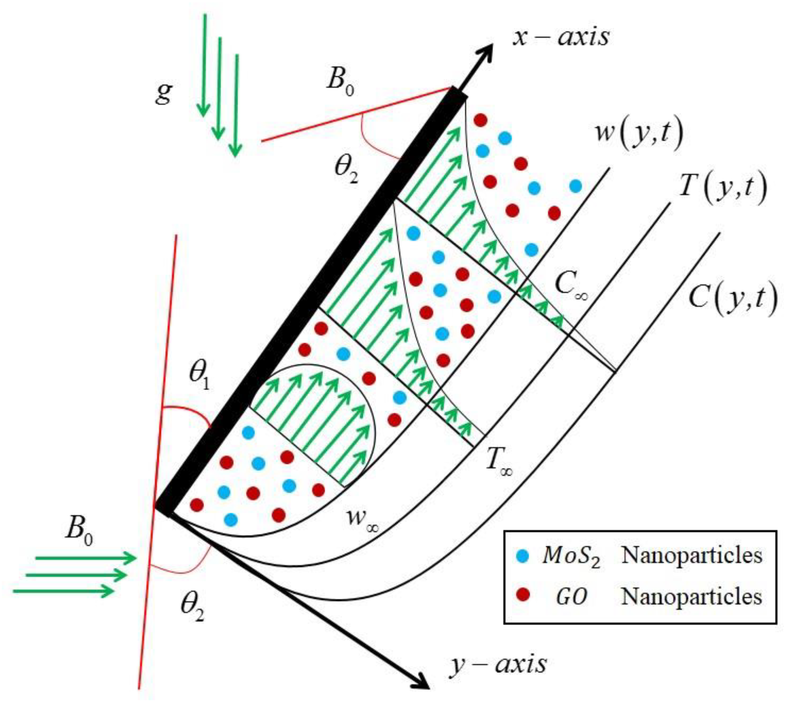
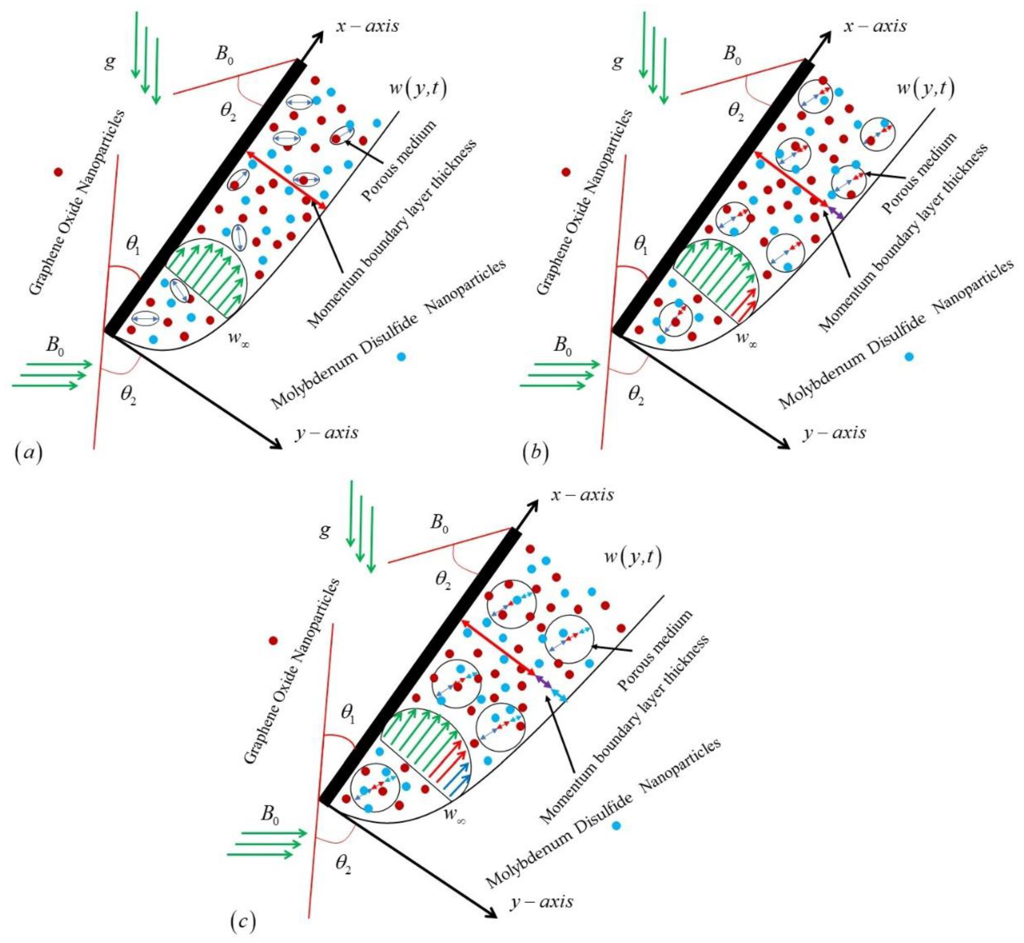
2. Mathematical Formulation

We investigate an unsteady, incompressible, free-convective MHD (magnetohydrodynamics) Casson nanofluid flow over an inclined plate as shown in Figure 1, which characterizes an asymmetrical behavior of the fluid flow and heat transfer with significant impacts of slip boundary conditions. The plate originated in the xy-plane with an inclination angle of θ 1 . The Newtonian heating effect, slip boundary, and porosity are also supposed in the respective boundary conditions and governed equations. Initially, at t = 0 , the plate and mixed suspension of two nanoparticles (MoS2 and GO) with CMC-based fluid form a distinct nanofluid. The thermophysical properties of these nanofluids are in thermal equilibrium. Moreover, the temperature and concentration are both constant with T and C , respectively. After some time t > 0 + , the inclined pored plate starts to oscillate with velocity U o H ( t ) C o s ( ω t ) . Due to vibrations and a temperature rise, the stationary fluid begins to flow on the pored oscillating plate with the same velocity as the vibrating plate. Moreover, it is assumed that the temperature, concentration and velocity are dependent over y and t. The mathematical representation of Casson fluid is defined in the following equation [57].
τ i j = { 2 ( μ γ + P y 2 π ) e i j     ;             π > π c   2 ( μ γ + P y 2 π c ) e i j     ;             π < π c
Here P y signifies the stress due to non-Newtonian fluid, μ represents the viscosity, π c shows the critical value of π and μ γ is flexible active viscosity.
Furthermore, the mathematical model of the respective problem can be originated with the help of Boussinesq’s approximations, as follows [32]:
ρ n f w ( y , t ) t = μ n f ( 1 + 1 β 1 * ) 2 w ( y , t ) y 2 + g ( ρ β T ) n f ( T ( y , t ) T ) c o s ( θ 1 )   σ n f B o 2 s i n ( θ 2 ) w ( y , t ) μ n f k w ( y , t ) + g ( ρ β C ) n f ( C ( y , t ) C ) c o s ( θ 1 )
( ρ C p ) n f T ( y , t ) t = δ ( y , t ) y ,       where             δ ( y , t ) = k n f T ( y , t ) y .
C ( y , t ) t = J ( y , t ) y ,       where             J ( y , t ) = D C ( y , t ) y .
Here,   δ ( y , t ) and J ( y , t ) denote the heat flux rate using Fourier’s as well as Fick’s law.

2.1. Boundary Conditions

The appropriate physical trustworthy boundary conditions for the given problem are:
w ( y , 0 ) = 0 ,                                       T ( y , 0 ) = T ,                                                 C ( y , 0 ) = C   ;                                 y 0
w ( 0 , t ) b w y | y = 0 = U o H ( t ) c o s ( ω t ) ,     T y | y = 0 = h k T ( 0 , t ) ,   C ( 0 , t ) = C + ( C w C ) ,       t > 0
w ( y , t ) 0 ,                                   T ( y , t ) T ,                       C ( y , t ) C                                 a s           y  

2.2. Non-Dimensional Parameters

To ease further the investigation of the given problem, here, we introduce the following dimensionless parameters:
y * = U o υ f y ,     w * = w U o ,     t * = U o 2 υ f t ,     T * = T ( y , t ) T T w T = T ( y , t ) T Δ T  
C * = C ( y , t ) C C w C = C ( y , t ) C Δ C ,                   q * = q q o ,               J * = J J o ,             ω * = ν f ω U o 2   ,       b * = U o ν f b .
Furthermore, ignore the steric notation and substitute the rest of the above parameters in the leading governing Equations (1) to (3) and boundary Conditions (4) to (6). Thus, the following non-dimensional governed equations are reduced as follows:
Ψ o w ( y , t ) t = Ψ 1 β 1 2 w ( y , t ) y 2 + Ψ 2 G r T ( y , t ) c o s ( θ 1 ) ( M   s i n ( θ 2 ) + Ψ 1 K ) w ( y , t ) + Ψ 3 G m   C ( y , t ) c o s ( θ 1 )
Ψ 4 P r   T ( y , t ) t = Ψ 5 2 T ( y , t ) y 2
Ψ 6 C ( y , t ) t = 2 C ( y , t ) y 2
With the subsequent non-dimensional conditions:
w ( y , 0 ) = 0 ,                   T ( y , 0 ) = 0 ,                     C ( y , 0 ) = 0   ;                   y 0 ,
w ( 0 , t ) b w y | y = 0 = H ( t ) c o s ( ω t ) ,               T y | y = 0 = ( 1 + T ( 0 , t ) ) ,           C ( 0 , t ) = 1
w ( y , t ) 0 ,                 T ( y , t ) 0 ,           C ( y , t ) 0                     a s           y  
In which:
Ψ 0 = ( 1 φ ) + φ ρ s ρ f ,     Ψ 1 = 1 ( 1 φ ) 2.5 ,     Ψ 2 = ( 1 φ ) + φ ( ρ β T ) s ( ρ β T ) f , Ψ 3 = ( 1 φ ) + φ ( ρ β c ) s ( ρ β c ) f ,     Ψ 4 = ( 1 φ ) + φ ( ρ C p ) s ( ρ C p ) f , Ψ 5 = 1 + 2 k f k s 2 φ ( k f k s 1 ) 1 + 2 k f k s + φ ( k f k s 1 ) ,           Ψ 6 = S c ,       β 1 = ( 1 + 1 β 1 * ) .

2.3. Dimensionless Parameters

The obtained similarity equations comprised distinct distinguished parameters which are symbolically defined as:
P r = ( μ C p ) f κ f ,     G r = g ( β T ) f Δ T ν f U o 3 ,       S c = υ f D ,     G m = g ( β c ) f Δ C ν f U o 3 ,             K = k U 0 ν f .
These parameters are respectively called the Prandtl number, the Grashof number for temperature, the Schmidt number, Grashof number for concentration and the dimensionless porosity parameter.

2.4. Thermophysical Properties of the Nanofluid

The leading governing equations comprised some more mathematical notations like ρ n f ,   μ n f ,   σ n f ,   k n f ,   ( ρ C p ) n f and ( ρ β ) n f , which are namely called the density, viscosity, electrical conductivity, thermal conductivity, heat capacity and thermal expansion coefficients of the NFs. The correlations of these NFs model are given in Table 1, while the experimental data of the respective base CMC fluid and distinct nanoparticles are given in Table 2.

2.5. Basic Preliminaries

The one-parametric Mittag–Leffler function is
E α ( z ) = n = 0 z n Γ ( α n + 1 ) ;             α , z , β ,       R e ( α ) > 0  
Mittag–Leffler has investigated this [63]. After some time, Wiman [64] investigated the two parametric Mittag–Leffler functions, a greater generalization of the one-parametric function.
E α , β ( z ) = n = 0 z n Γ ( α n + β ) ;             α , z , β ,       R e ( α ) > 0
The three-parametric Mittag–Leffler function, also discussed as the Prabhakar fractional derivative, was first presented by Prabhakar in [65].
E α , β γ ( z ) = n = 0 ( γ ) n z n n !   Γ ( α n + β ) ;             α , β , γ , z ,       R e ( α ) > 0
With the basic properties
E α ( z ) = E α , 1 1 ( z ) ,         E α , β ( z ) = E α , β γ ( z ) ,       E 1 , 1 1 ( z ) = exp ( z )
{ t β 1   E α , β γ ( α t α ) } = q β ( 1 α q α ) γ
(Prabhakar kernel) The function
e α , β γ ( α ; t ) = t β 1   E α , β γ ( α t α ) ;           t ,         α , β , γ , z  
is the Prabhakar kernel.
(Prabhakar Integral) The Prabhakar integral is expressed as [66,67]
E α , β , α γ f ( t ) = e α , β γ ( α ; t ) f ( t ) = 0 t ( t τ ) β 1   E α , β γ ( α ( t τ ) α ) f ( τ ) d τ  
with its Laplace
{ E α , β , α γ f ( t ) } ( q ) = { e α , β γ ( α ; t ) } { f ( t ) } = q α γ β ( q α α ) γ { f ( t ) }
Some suitable fractional constraint cases can be summarized as
If
β = γ = 0
If
β = 1 ,     γ = 0 1 { { e α , 1 0 ( α ; t ) } } = 1 { 1 q } = 1  
If
β > 0 ,     γ = 0 1 { { e α , β 0 ( α ; t ) } } = 1 { 1 q β } = t β 1 Γ ( β )  
when β > 0 ,   α = 0 , then property three will repeat as
{ e α , β γ ( 0 ) } = q β
(The regularized Prabhakar derivative) In [66,67], regularized Prabhakar derivative is specified as
D   C α , β , α γ g ( t ) = E α , m β , α γ g m ( t ) = e α , m β γ ( α ; t ) g m ( t ) = 0 t ( t τ ) m β 1 E α , m β γ ( α ( t τ ) α ) g m ( τ ) d ( τ )
where g m is the mth derivative of g ( t ) , and D   C α , β , α γ denotes the Prabhakar derivative operator (t). Equations (15) and (16) can be used to generate the generalized Prabhakar’s Laplace and its kernel, as below:
{ D   C α , β , α γ g ( t ) } = { e α , m β γ ( α ; t ) g m ( t ) } { g m ( t ) } = q β m ( 1 α q α ) γ { g m ( t ) } { e α , m β γ ( α ; t ) } = q β m ( 1 α q α ) γ
The Prabhakar derivative D   C α , 1 , α 0   g ( t ) = g ( t ) with its kernel is equal to h ¯ p ( α , 1 , 0 , α , q ) = d d t ( g ( t ) ) for β = 1 ,   γ = 0 ,   m = 1 . Because the LT of Prabhakar’s fractional operator D   C α , β , α γ follows
[ D   C α , β , α γ   h ( t ) ] = [ h m ( t ) e α , m β γ ( α ; t ) ] = { h m ( t ) } { e α , m β γ ( α ; t ) } = { h m ( t ) } s β m ( 1 α s α ) γ
we might obtain the traditional Fourier’s rule by assuming β = γ = 0 . The following Fourier’s and Fick’s laws also apply to the Prabhakar derivative since Fourier’s law effectively defines the Prabhakar fractional derivative
δ ( y , t ) = D   C α , β , α γ T ( y , t ) y
J ( y , t ) = D   C α , β , α γ C ( y , t ) y

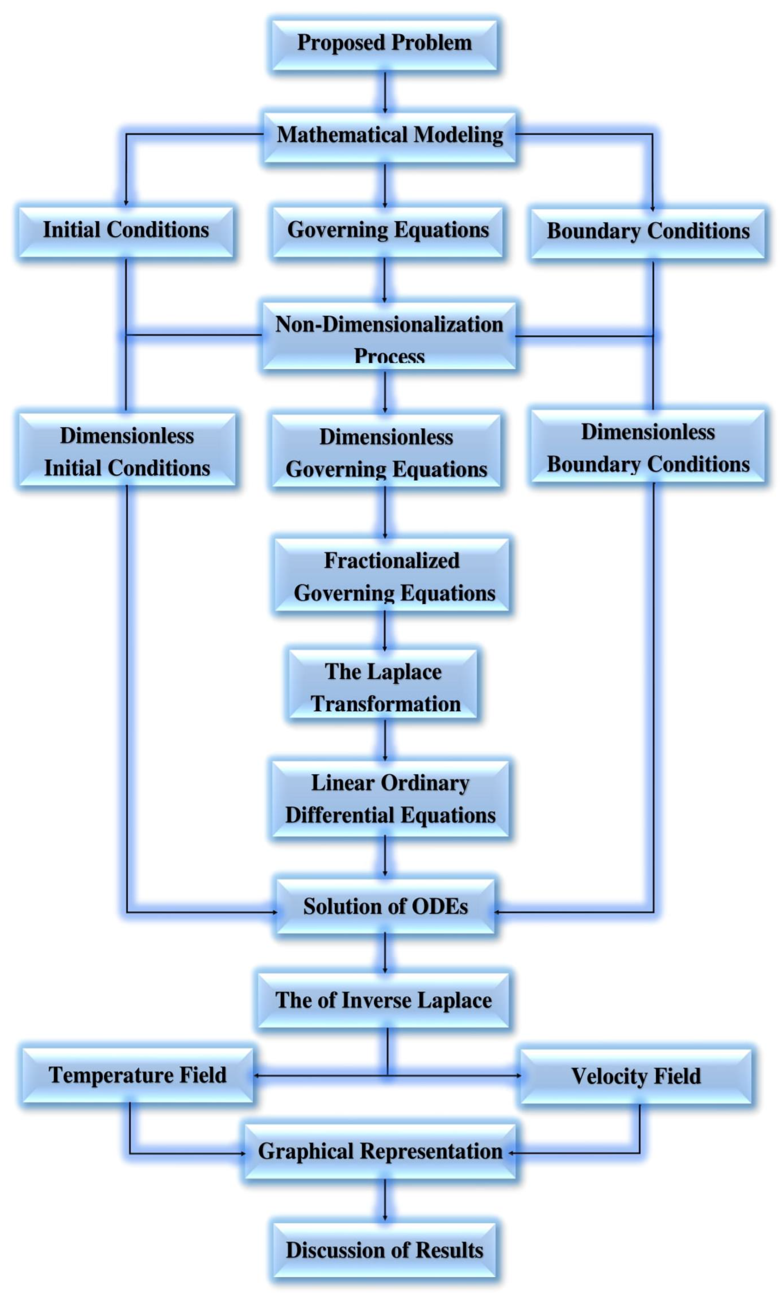
3. Solution of the Fractional Model

This section is basically devoted to explaining the working procedure of the fractional models for the acquired equations.

3.1. Solution of the Energy Field

Since the Fourier law of thermal flux is a component of the energy equation, the energy profile can be solved using the LT scheme on Equations (8) and (18) and the accompanying conditions:
Ψ 4 P r   s   T ¯ ( y , s ) = Ψ 5 δ ¯ ( y , s ) y
δ ¯ ( y , s ) = ( s β ( 1 α s α ) γ ) T ¯ ( y , t ) y
T ¯ y | y = 0 = ( 1 s + T ¯ ( 0 , s ) ) , T ¯ ( y , s ) 0 ; y .
Equation (21) is introduced into Equation (20) for the temperature field solution
Ψ 5 d 2 T ¯ ( y , s ) d y 2 = Ψ 4 P r   s 1 β ( 1 α s α ) γ T ¯ ( y , s ) .
Utilizing the conditions mentioned above and resolving the ordinary differential equation (Equation (23)), the heat flux solution will result as:
T ¯ ( y , s ) = 1 Ψ 4 P r Ψ 5   s 1 β ( 1 α s α ) γ 1   e y Ψ 4 P r Ψ 5   s 1 β ( 1 α s α ) γ s   .
We shall employ numerical techniques, such as Stehfest’s as well as Tzou’s systems in Table 3, to determine the inverse of Laplace of Equation (24).

3.2. Classical Simulations for Temperature Profile ( β = γ = 0 )

For classical heat transport by taking β = γ = 0 , so
[ e α , 0 0 ( α ; t ) ] = 1 = δ ( t ) .
The Dirac’s Delta distribution is represented by δ ( t ) . The classical Fourier’s law will be created by utilizing this to convert the generalized Fourier’s law. So
T ¯ ( y , s ) = 1 Π 1   s 1   e y Π 1   s s  
with its Laplace inverse
T ( y , t ) = H 1 H 2 , H 1 = 1 π t + e t Π 1 E r f ( t Π 1 ) Π 1 ,   H 2 = E r f ( Π 1 y 2 t ) .  

3.3. Solution of the Concentration Field

By using the LT on Equations (9) and (19) for the equation of the concentration profile and on its stable conditions, one can make the concentration profile comparable to the thermal profile.
Ψ 6   s   C ¯ ( y , s ) = J ¯ ( y , s ) y
J ¯ ( y , s ) = ( s β ( 1 α s α ) γ ) C ¯ ( y , s ) y
C ¯ ( 0 , s ) = 1 s , C ¯ ( y , s ) 0 ; y
Presenting Equation (26) into (27), for the simulations of the concentration field
2 C ¯ ( y , s ) y 2 Ψ 6 s 1 β ( 1 α s α ) γ C ¯ ( y , s ) = 0
By utilizing the above condition, the solution of the concentration profile will become as follows:
C ¯ ( y , s ) = 1 s   e y Ψ 6     s 1 β ( 1 α s α ) γ
Again, Table 3 will employ numerical approaches like Stehfest’s and Tzou’s algorithms for the inverse of Laplace of Equation (30).

3.4. Classical Solution of Concentration Field ( β = γ = 0 )

For classical concentration results, by taking β = γ = 0 , then
[ e α , 0 0 ( α ; t ) ] = 1 = δ ( t ) ,
C ¯ ( y , s ) = 1 s   e y Ψ 6   s .
With its Laplace inverse
C ( y , t ) = E r f c [ Ψ 6 y 2 t ] ,               Ψ 6 , y > 0  

3.5. Solution of the Momentum Field

The method utilized to solve the momentum equation for the energy and concentration equations will be applied in this section as well. Using the appropriate conditions in Equation (7) and the LT method, we obtain
Ψ 1 β 1 2 w ¯ ( y , s ) y 2 ( M   s i n ( θ 2 ) + Ψ 1 K + Ψ o s ) w ¯ ( y , s ) = Ψ 2 G r T ¯ ( y , s ) C o s ( θ 1 ) Ψ 3 G m   C ¯ ( y , s ) C o s ( θ 1 ) ,
w ¯ ( 0 , s ) b w ¯ y | y = 0 = s ω 2 + s 2 , w ¯ ( y , s ) 0 ; y
Under these assumptions, the velocity equation’s solution will take the form
w ¯ ( y , s ) = 1 1 + b 1 Π 1 ( Π 4 + Ψ o s ) ( Π 5 s ( Π 7   s 1 β ( 1 α s α ) γ     1 ) 1 + b Π 7   s 1 β ( 1 α s α ) γ ( Π 7   s 1 β ( 1 α s α ) γ ) 1 Π 1 ( Π 4 + Ψ o s ) + Π 6 s 1 + b Ψ 6   s 1 β ( 1 α s α ) γ   ( Ψ 6   s 1 β ( 1 α s α ) γ ) 1 Π 1 ( Π 4 + Ψ o s ) + s ω 2 + s 2 ) e y 1 Π 1 ( Π 4 + Ψ o s ) Π 5 s ( Π 7   s 1 β ( 1 α s α ) γ     1 ) e y Π 7   s 1 β ( 1 α s α ) γ ( Π 7   s 1 β ( 1 α s α ) γ ) 1 Π 1 ( Π 4 + Ψ o s ) Π 6 s e y Ψ 6   s 1 β ( 1 α s α ) γ   ( Ψ 6   s 1 β ( 1 α s α ) γ ) 1 Π 1 ( Π 4 + Ψ o s ) .
where
Π 1 = Ψ 1 β 1 ,                 Π 2 = M   s i n ( θ 2 ) ,                       Π 3 = Ψ 1 K ,                       Π 4 = Π 2 + Π 3 , Π 5 = Ψ 2 G r   C o s ( θ 1 ) ,                             Π 6 = Ψ 3 G m   C o s ( θ 1 ) ,                       Π 7 = Ψ 4 P r Ψ 5 .
Various authors have employed various numerical inverse techniques to determine the Laplace inverse. So that we can numerically examine the temperature and velocity profile, we will also apply the Stehfest algorithm here. Mathematically, the Gaver–Stehfest algorithm [68] is defined as
w ( ξ , t ) = l n ( 2 ) t   n = 1 N v n   w ¯ ( ξ , n l n ( 2 ) t )
where N is a positive integer, and
v n = ( 1 ) n + N 2 r = [ q + 1 2 ] m i n ( q , N 2 ) r N 2   ( 2 r ) ! ( N 2 r ) ! r !   ( r 1 ) !   ( q r ) !   ( 2 r q ) !  
We employed Tzou’s approach, another estimation for the formulation of the temperature as well as a velocity field, for the legitimacy and verification of our obtained numerical results using the Stehfest technique. Tzou’s method can be described as mathematical:
w ( ξ , t ) = e 4.7 t   [ 1 2 w ¯ ( r , 4.7 t ) + R e   { j = 1 N ( 1 ) k   w ¯ ( r , 4.7 + k π i t ) } ] .

3.6. Gradients

In this paper, the following three important key engineering quantities of interest are used like the Nusselt number, the Sherwood number and the shear stress. These gradients are mathematically expressed as:
N u = T ( y , t ) y | y = 0 = 1 { T ¯ ( 0 , s ) y } ,
S h = C ( y , t ) y | y = 0 = 1 { C ¯ ( 0 , s ) y } ,
C f = w ( y , t ) y | y = 0 = 1 { w ¯ ( 0 , s ) y } .

4. Results with Discussion

Casson fluid fractional model with free-convective NF-containing molybdenum disulfide (MoS2) plus base fluid and graphene-oxide (GO) as nanoparticles with the suspension of Carboxy-Methyl Cellulose (CMC) as base fluid with porosity, inclined magnetic field, Newtonian heating on temperature, and slip boundary condition on velocity are studied in this article. These nanoparticles have unique thermo-physical properties, as shown in Table 1. The use of the most current definition of fractional derivative, namely, the Prabhakar fractional derivative, distinguishes this study. The dimensionless defined fractional model issue for velocity, temperature, and concentration profiles is addressed using the LT approach, and Stehfest’s and Tzou’s methods are used for Laplace inversion. For detailed knowledge of the extensive importance of the considered flow problem, graphs are depicted including physical parameters as α ,   β ,   γ ,   P r ,   G r ,   S c ,   G m ,   M ,   θ 2 ,   b ,   K ,   β 1 and φ. In addition, a flowchart (see Figure 2) has been included in the report to help illustrate the entire situation of the research effort. In addition, graphical demonstrations for temperature field, concentration, and velocity are provided in Figure 3, Figure 4, Figure 5, Figure 6, Figure 7, Figure 8, Figure 9, Figure 10, Figure 11, Figure 12 and Figure 13 by changing the values of α ,   β ,   γ   , and other essential system parameters.
Figure 3a,b portrays the physical effect of fractional parameters ( α ,   β ,   γ ) and P r on the temperature. It is represented that the temperature displays a declining behavior of ( α ,   β ,   γ ) and P r . It has also been noted that, for both parameters, the maximum temperature is at y = 0 and, after converging, becomes zero for y . It has been described that, for greater P r , the temperature is dropping. In general, the consistency of the temperature boundary layer lays down quickly with growing P r , as this temperature is linearly declined, due to greater viscosity and thickness of the fluid. Furthermore, in the comparison of nanofluids, ( C M C / M o S 2 ) -based fluid has a bit more heat flow rate as compared to ( C M C / G O ) due to the thermophysical characteristics of the considered nanomaterials.
Figure 4a,b reveals the physical impact of α ,   β ,   γ , and S c on the concentration field. It is signified that the concentration profile shows a lessening behavior for α ,   β ,   γ , and S c . The methodology behind this is that the boundary layer of concentration is decreased when growing the values of S c . Concentration is an essential factor of the velocity field on the movement of the fluid that cannot be ignored.
Figure 5a,b exposes the impact of α ,   β ,   γ , and P r on the velocity field for different values of different constraints. It is implied that the velocity profile shows a decreasing behavior for α ,   β ,   γ , and P r . This means that we can compute the thermal or momentum profiles for any value of the fractional parameter known as the memory effect. As a result, the fractional parameter is really the memory parameter. The trend of the velocity profile is shown in Figure 6a by growing the G r . An even more significant consequence is that growing the G r increases the fluid’s speed. As G r increases, the peak values of the velocity also rise quickly towards the porous plate before gently descending to the free-stream velocity. Physically, lower G r values indicate more viscosity and growing the G r variates the bouncy forces and thickens the velocity layer and enhances fluid motion. Once again, like the temperature profile, the nanofluid mixed with ( M o S 2 ) nanoparticles has a greater impact on the momentum profile as compared to ( G O ) nanoparticles. Figure 6b defines the impact of G m by taking the changing values of G m on the momentum profile. The ratio of buoyancy force to viscous force is called the mass Grashof number of those reasons to clear convection. From these diagrams, it is portrayed that the velocity profile is elevated for growing G m .
Figure 7a signifies the influence of the magnetic field M on the fluid velocity. The velocity is decreased by M . It should be observed that the magnetic field impacts the velocity field by producing a drag force that opposes the motion of the fluid, causing a reduction in velocity. While the flow rate near the moving inclined plate surface drops, an increase in the M in this case only marginally delays the fluid’s trip away from the moving inclined plate surface and toward the free-stream velocity. The actual fact that the Lorentz force created in the current flow model as a result of the interaction between the transverse magnetic field and the fluid velocity works as a resistive force to the fluid flow that helps to slow the flow is in remarkable accord with this phenomenon. Physically, a rise in the magnetic field increases Lorentz’s force, which declines the velocity. Figure 7b shows that the velocity contour decreased by increasing α ,   β ,   γ with slip conditions. Further, we have noted that the growing slip parameter b enlarges the velocity. Figure 8a signifies the trend of the inclination angle θ 2 of the magnetic field on the velocity. The growth in the θ 2 decays the impact of M , which takes off the influence of Lorentz force; so by rising the estimation of θ 2 , the velocity again declines. Figure 8b shows that the velocity is decreased by enlarging the porosity parameter 𝐾. Furthermore, for the porosity parameter, physically, when in the porous medium, the holes are significantly enough, and then the resistance of the porousness can be discounted. So, the velocity rises as the presence of the porous surface advances the resistance to the fluid.
Figure 9a expresses that the velocity is directly proportional to the Casson parameter β 1 . The stream zone, where more distinct peak values were recorded, is where velocity is at its highest close to the plate before decreasing away from it. As the estimates of Sc rise, kinematic viscosity rises, and mass diffusivity declines, as shown in Figure 9b, the velocity is inversely proportional to Sc. The velocity profile is shown in Figure 10a for various estimates of φ. This plot further shows that the thickness of the thermal boundary layer is reduced as increasing values of the directing parameter φ, which causes the velocity of the nanofluid to decrease. Additionally, as the number increases, the fluid becomes more viscous. The science behind this is that raising the volume fraction increases the thermal conductivity of Casson nanofluid, which increases the thickness of the boundary layer and hence reduces fluid velocity. Furthermore, compared to the G O -CMC-based NF, the M O S 2 -CMC-based nanoparticle fluid has a higher temperature, concentration, and velocity profiles. These innovative annotations may present numerous applications in enlightening the thermal capacity of numerous engineering and industrial phenomena. Figure 10b is sketched to compare different nanofluids on the velocity profile. The effects on the velocity of other nanofluids are lesser than the velocity of M O S 2 -CMC nanofluid, and this influence is reversed after a specific value of y .
We compare our results for temperature and velocity in Figure 11a and Figure 12a using the numerical approaches of Stehfest and Tzou (a). The fact that the curves of the two procedures appear to overlap confirms our obtained results’ validity. Table 3 examines the numerical analysis of the temperature, concentration, and velocity profiles using the Stehfest and Tzou numerical methods. The Nusselt number is a significant physical quantity. The Nusselt number quantifies the influence of volume fraction on the flow of a nanofluid and its heat transfer rate. Table 4 displays the Nusselt number, Sherwood number and skin friction analysis. In order to assess the reliability of our obtained data, Tassaddiq et al.’s [32] results for temperature and velocity profiles are compared in Figure 11b and Figure 12b, respectively. These graphs make it evident that our findings overlap with those of Tassaddiq et al. [32]. Figure 13a–c show geometrically the variation of the velocity profiles for the distinct cases of the porosity parameter. From the graphs, it is seen that the boundary layer thickness escalates with higher improvement in the porosity parameter while the velocity profile declines.

5. Conclusions

The unsteady and inviscid nanofluid solution, including ( M O S 2 ) and ( G O ) as nanoparticles and (CMC) as the base fluid, was investigated in this study as it flows over an angled oscillating plate. The study was analyzed for two nanofluids: (MoS2/CMC) nanofluid and (GO/CMC) nanofluid. For the solution of the dimensionless guided model, the Prabhakar fractional derivative, a new and updated definition of fractional derivatives, was used. Using numerical approaches, such as Stehfest’s and Tzou’s, momentum solves the problem by exploiting the integral transform scheme LT. Leading equations are studied graphically and quantitatively at various points to assess the effects of various restrictions on them. Bullets can be used as one of the direct results of graphical and numerical representation.
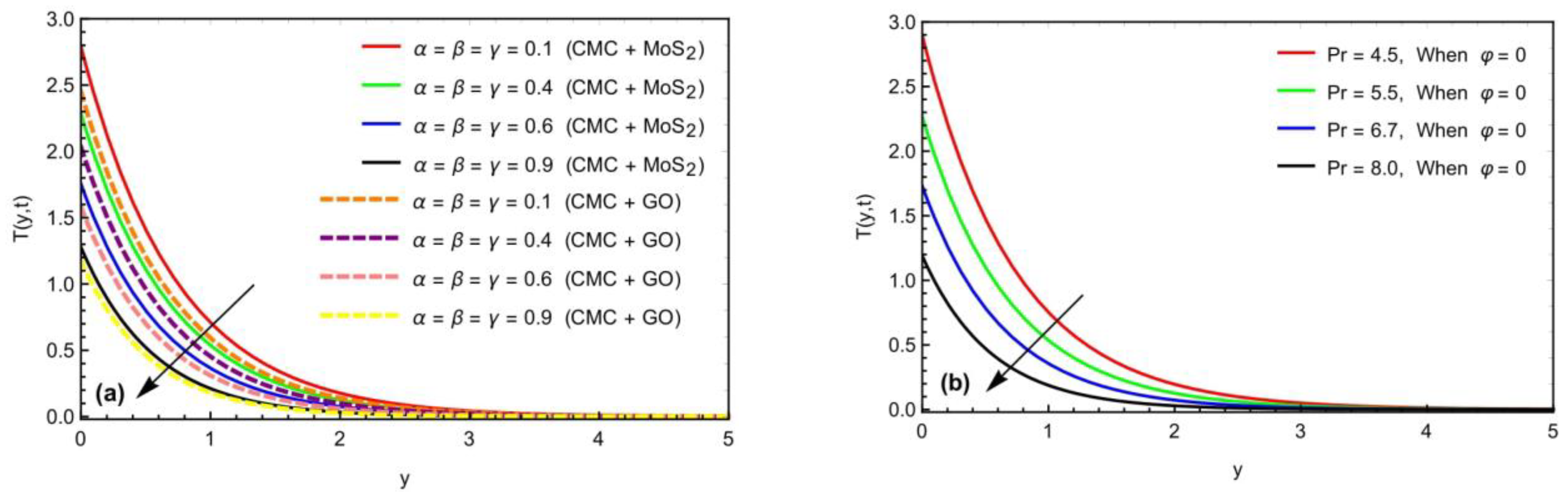
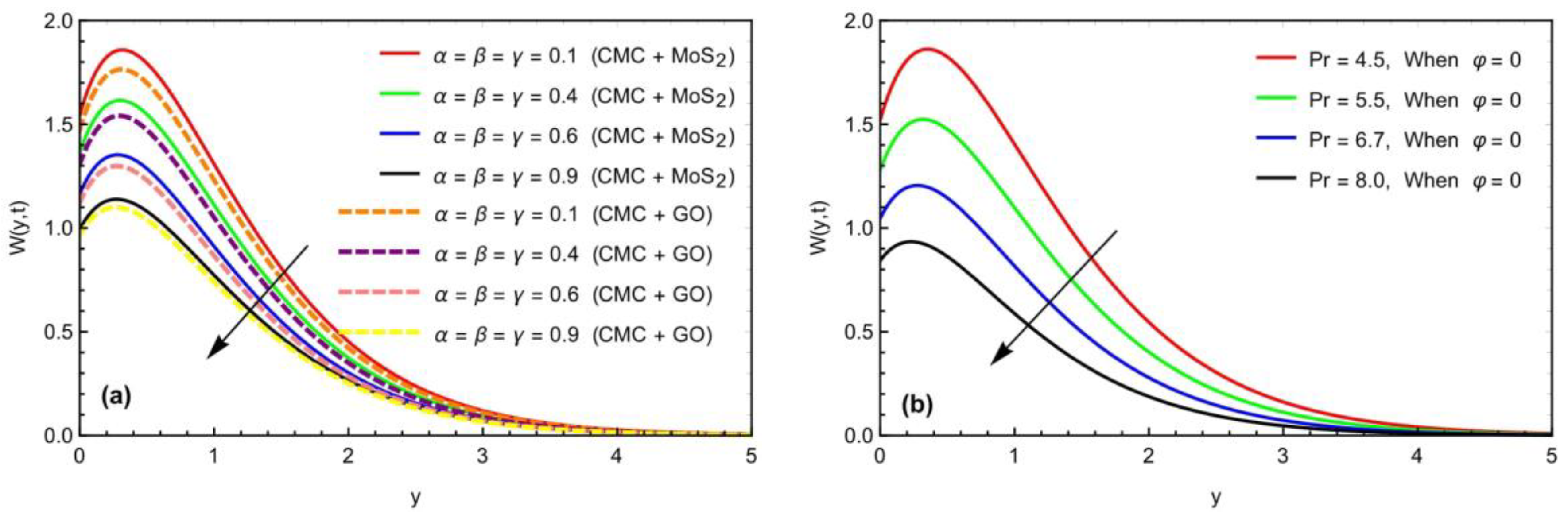
  • The temperature field falls as the Prabhakar fractional limitations increase, asymptotically rising with time.
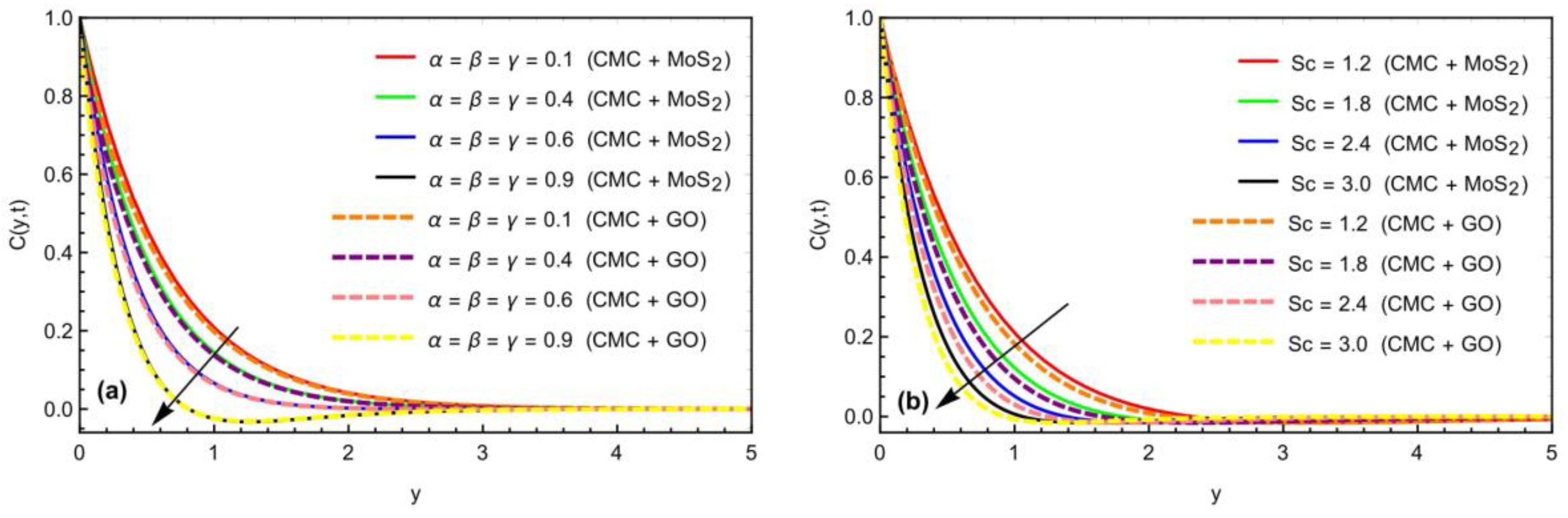
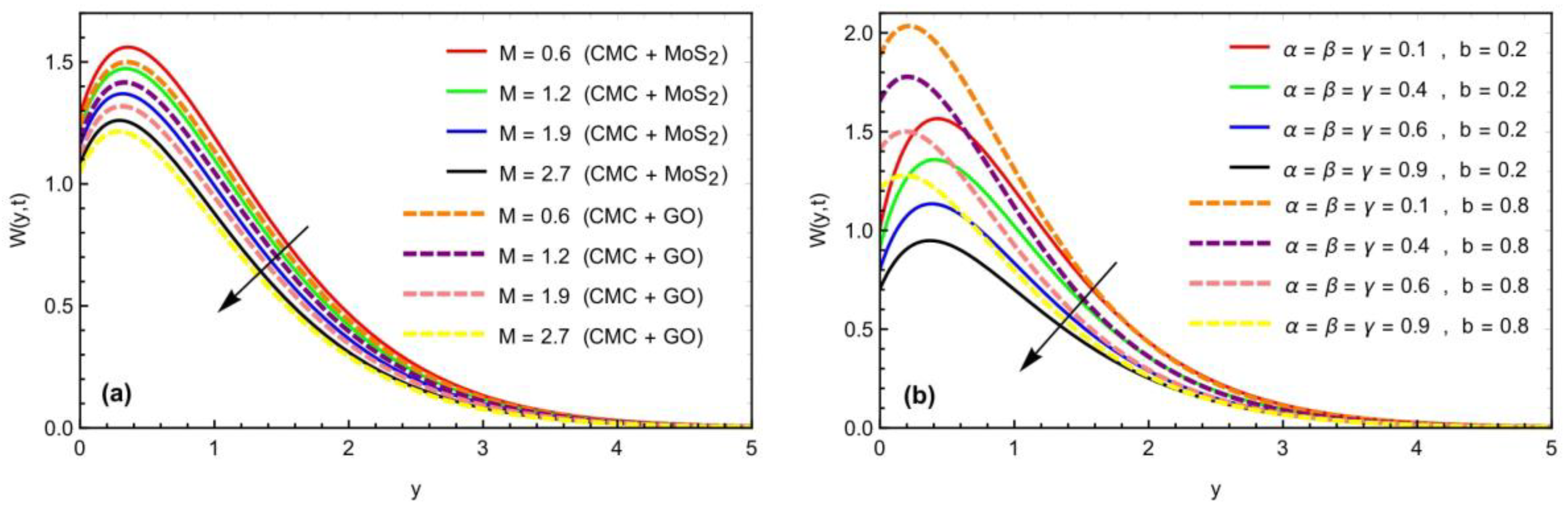
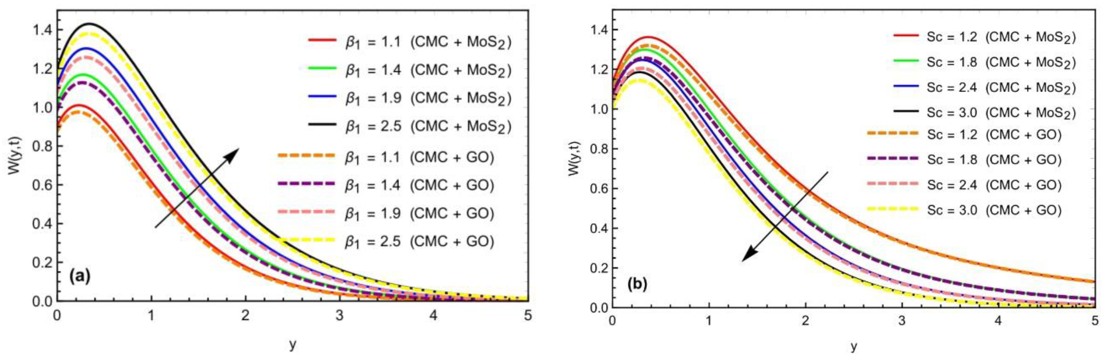
  • With an increase in the values of the fractional limitations, the velocity and concentration profiles likewise begin to drop.
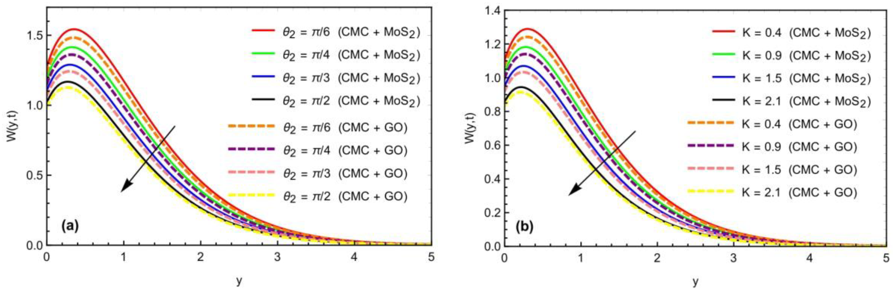
  • Improvement in porous constraint will decline the fluid velocity with an increase in momentum boundary layer thickness (see Figure 13).
  • It should be noticed that the flow rate exhibited the same behavior for both slip and zero-slip situations for both traditional and fractional formulations.
  • Selecting an appropriate value of the Prabhakar fractional parameters may govern the speed of the flowing nanofluid.
  • The momentum and thermal fields slow down with the increment in Prandtl number values.
  • It is clear that, when slip or no-slip circumstances exist, the flow rate decreases under increased values for the fractional factors.
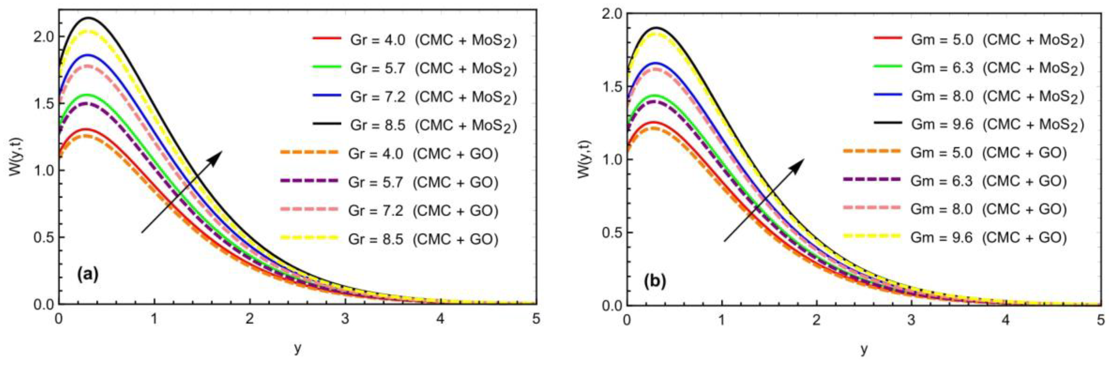
  • The fluid flows more progressively with the enhancement of the mass and heat Grashof number.
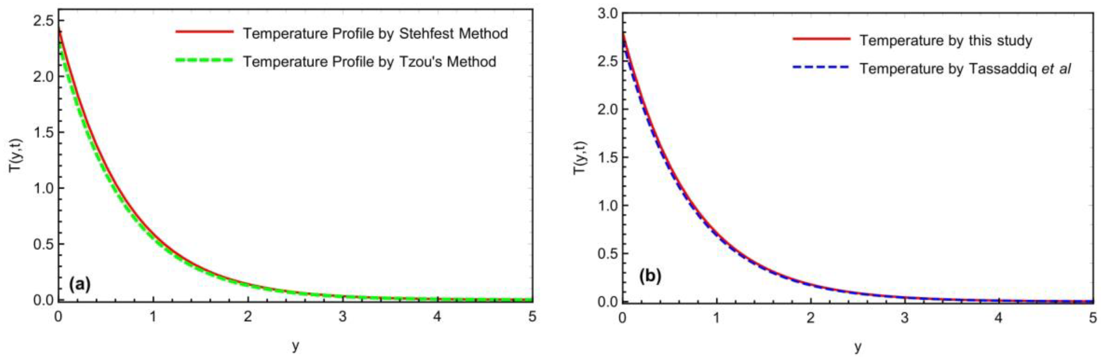
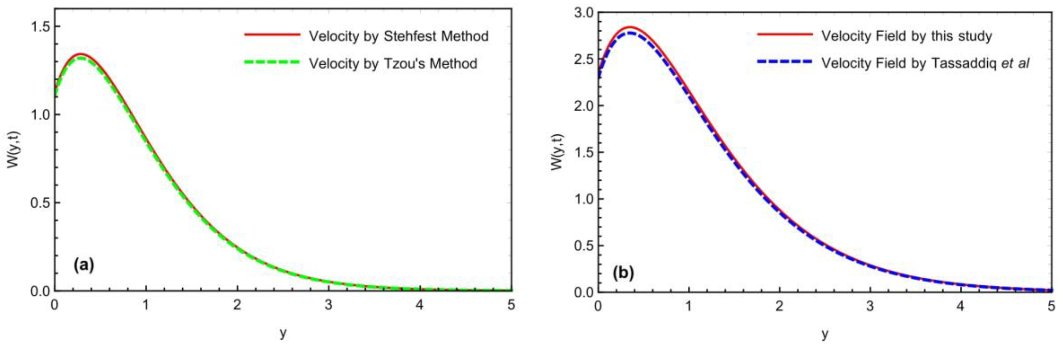
  • The solution curves of the two numerical schemes coincide, validating our attained results. Furthermore, the velocity accelerates by increasing the values of the heat and mass Grashof numbers due to the buoyancy effect.
  • The stream zone, where more distinct peak values were recorded, is where velocity is at its highest close to the plate before decreasing away from it.
  • The fluid motion can be controlled with the help of an external applied magnetic field, whose strength is maximum at the right angle.
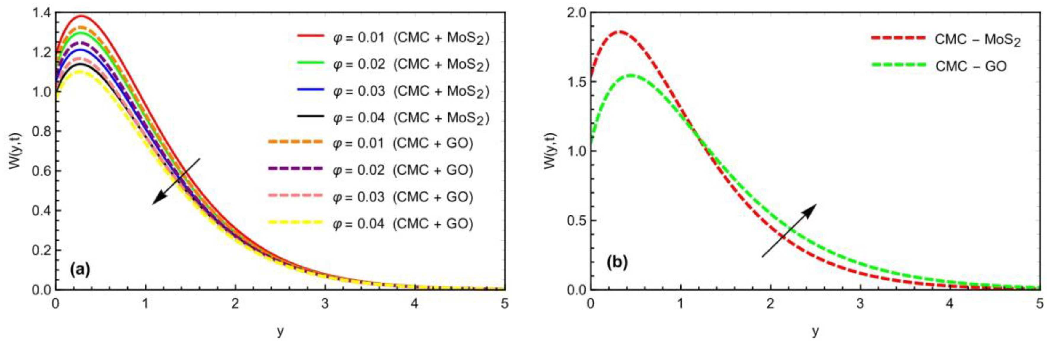
  • The velocity field of nanofluid mixed with ( M o S 2 ) nanoparticles is more remarkable than the nanofluid mixed with ( G O ) nanoparticles.
  • The validity of velocity profile findings in graphical form is also indicated by comparing our acquired velocity solution with Tassaddiq et al. [32].
  • The Prabhakar fractional model becomes classical by taking the fractional constraints as α ,   β ,   γ 1 .
Recent advances in the study of fractional order frameworks include the fractional natural decomposition method (FNDM), the fractional Shehu transform, and the modified generalized Taylor fractional series method (MGTFSM). Researchers in the future can correlate their findings to those we found utilizing the Caputo–Fabrizio, Atangana–Baleanu, and Prabhakar fractional methods in our investigation.

Author Contributions

Conceptualization, S.M.E., A.R. and U.K.; methodology, S.M.E., A.R. and U.K.; software, S.M.E., A.R., Z.R. and U.K.; validation, S.M.E., A.R., U.K., S.E. and A.M.A. (Ahmed M. Abed).; formal analysis, A.M.A. (Abeer M. Alotaibi), S.E., A.R., A.M.A. (Ahmed M. Abed) and Z.R.; investigation, U.K., A.M.A. (Abeer M. Alotaibi), S.E., Z.R. and A.M.A. (Ahmed M. Abed); resources, A.M.A. (Abeer M. Alotaibi); data curation, Z.R.; writing—original draft preparation, U.K., A.M.A. (Abeer M. Alotaibi), S.E. and A.M.A. (Ahmed M. Abed); writing—review and editing, Z.R., A.M.A. (Abeer M. Alotaibi) and A.M.A. (Ahmed M. Abed); visualization, Z.R., A.R., A.M.A. (Ahmed M. Abed) and S.E.; supervision, U.K.; project administration, S.M.E.; funding acquisition, S.M.E. and Z.R. All authors have read and agreed to the published version of the manuscript.

Funding

The author expresses her gratitude to the Deanship of Scientific Research at King Khalid University, Abha, Saudi Arabia, for funding this work through the Research Group Project under Grant Number (RGP.2/154/43). Also, this work was supported by the Princess Nourah bint Abdulrahman University Researchers Supporting Project number (PNURSP2022R163), Princess Nourah bint Abdulrahman University, Riyadh, Saudi Arabia.

Institutional Review Board Statement

Not applicable.

Informed Consent Statement

Not applicable.

Data Availability Statement

Not applicable.

Acknowledgments

The author (Z. Raizah) extends her appreciation to the Deanship of Scientific Research at King Khalid University, Abha, Saudi Arabia, for funding this work through the Research Group Project under Grant Number (RGP.2/154/43). Additionally, the authors are thankful to the support of Princess Nourah bint Abdulrahman University Researchers Supporting Project Number (PNURSP2022R163), Princess Nourah bint Abdulrahman University, Riyadh, Saudi Arabia.

Conflicts of Interest

The authors declare no conflict of interest.

Nomenclature

θ 1 -Angle of inclination of the plate [-]
θ 2 -Angle of inclination of magnetic field [-]
g -Acceleration due to gravity [ L T 2 ]
C -Concentration of the fluid [ M L 3 ]
U o -Constant velocity [ L T 1 ]
β 1 -Casson fluid parameter [-]
K -Dimensionless porosity parameter [-]
μ -Dynamic viscosity [ M L 1 T 1 ]
σ -Electrical conductivity [ S L 1   o r   M 1 L 2 T 3 A 2 ]
T w -Fluids temperature at the plate [ K ]
C w -Fluids Concentration at the plate [ M L 3 ]
G r -Heat Grashof number [-]
υ f -Kinematic viscosity [ L 2 T 1 ]
s -Laplace transformed variable [-]
G m -Mass Grashof number [-]
D -Mass diffusion coefficient [ L 2 T 1 ]
N u -Nusselt number [-]
P r -Prandtl number [-]
α , β , γ Prabhakar-fractional derivative operators [-]
k -Permeability of the porous medium [L]
S c -Schmidt number [-]
b -Slip parameter [-]
C f -Skin friction [-]
C p -Specific heat at constant pressure [ J M 1 K 1 ]
t -Time [ T ]
T -Temperature [ K ]
T -Temperature of fluid away from the plate [ K ]
w -Velocity [ L T 1 ]
Note: This [-] represents the dimensionless quantity.

References

  1. Miller, K.S.; Ross, B. An Introduction to the Fractional Calculus and Fractional Differential Equations; Wiley: New York, NY, USA, 1993. [Google Scholar]
  2. Gemant, A. XLV. On fractional differentials. Lond. Edinb. Dublin Philos. Mag. J. Sci. 1938, 25, 540–549. [Google Scholar]
  3. Blair, G.S.; Caffyn, J. VI. An application of the theory of quasi-properties to the treatment of anomalous strain-stress relations. Lond. Edinb. Dublin Philos. Mag. J. Sci. 1949, 40, 80–94. [Google Scholar] [CrossRef]
  4. Machado, J.T.; Kiryakova, V.; Mainardi, F. Recent history of fractional calculus. Commun. Nonlinear Sci. Numer. Simul. 2011, 16, 1140–1153. [Google Scholar] [CrossRef] [Green Version]
  5. Liouville, J. Memoir on some questions of geometry and mechanics, and on a new kind of calculation to solve these questions. J. L’école Pol. Tech. 1832, 13, 1–69. [Google Scholar]
  6. De Oliveira, E.C.; Tenreiro Machado, J.A. A review of definitions for fractional derivatives and integral. Math. Probl. Eng. 2014, 2014, 238459. [Google Scholar] [CrossRef] [Green Version]
  7. Kong, F.; Zhang, Y.; Zhang, Y. Non-stationary response power spectrum determination of linear/non-linear systems endowed with fractional derivative elements via harmonic wavelet. Mech. Syst. Signal Process. 2022, 162, 108024. [Google Scholar] [CrossRef]
  8. Saqib, M.; Mohd Kasim, A.R.; Mohammad, N.F.; Chuan Ching, D.L.; Shafie, S. Application of fractional derivative without singular and local kernel to enhanced heat transfer in CNTs nanofluid over an inclined plate. Symmetry 2020, 12, 768. [Google Scholar] [CrossRef]
  9. Rüdinger, F. Tuned mass damper with fractional derivative damping. Eng. Struct. 2006, 28, 1774–1779. [Google Scholar] [CrossRef]
  10. Agrawal, O.P. Analytical solution for stochastic response of a fractionally damped beam. J. Vib. Acoust. 2004, 126, 561–566. [Google Scholar] [CrossRef]
  11. Diethelm, K. The Analysis of Fractional Differential Equations; Lecture Notes in Mathematics; Springer: Berlin/Heidelberg, Germany, 2010; Volume 2004. [Google Scholar]
  12. You, X.; Li, S. Fully Developed Opposing Mixed Convection Flow in the Inclined Channel Filled with a Hybrid Nanofluid. Nanomaterials 2021, 11, 1107. [Google Scholar] [CrossRef]
  13. Trujillo, J.J.; Scalas, E.; Diethelm, K.; Baleanu, D. Fractional Calculus: Models and Numerical Methods; World Scientific: Singapore, 2016; Volume 5. [Google Scholar]
  14. Ogudo, K.A.; Muwawa Jean Nestor, D.; Ibrahim Khalaf, O.; Daei Kasmaei, H. A device performance and data analytics concept for smartphones’ IoT services and machine-type communication in cellular networks. Symmetry 2019, 11, 593. [Google Scholar] [CrossRef] [Green Version]
  15. Zhou, Y.; Shangerganesh, L.; Manimaran, J.; Debbouche, A. A class of time-fractional reaction-diffusion equation with nonlocal boundary condition. Math. Methods Appl. Sci. 2018, 41, 2987–2999. [Google Scholar] [CrossRef]
  16. Abbaszadeh, M. Error estimate of second-order finite difference scheme for solving the Riesz space distributed-order diffusion equation. Appl. Math. Lett. 2019, 88, 179–185. [Google Scholar] [CrossRef]
  17. Liu, F.; Liang, Z.; Yan, Y. Optimal convergence rates for semidiscrete finite element approximations of linear space-fractional partial differential equations under minimal regularity assumptions. J. Comput. Appl. Math. 2019, 352, 409–425. [Google Scholar] [CrossRef] [Green Version]
  18. Khan, I.; Raza, A.; Shakir, M.A.; Al-Johani, A.S.; Pasha, A.A.; Irshad, K. Natural convection simulation of Prabhakar-like fractional Maxwellfluid flowing on inclined plane with generalized thermal flux. Case Stud. Therm. Eng. 2022, 35, 102042. [Google Scholar] [CrossRef]
  19. Raza, A.; Thumma, T.; Al-Khaled, K.; Khan, S.U.; Ghachem, K.; Alhadri, M.; Kolsi, L. Prabhakar fractional model for viscous transient fluid with heat and mass transfer and Newtonian heating applications. Waves Random Complex Media 2022, 1–17. [Google Scholar] [CrossRef]
  20. Jie, Z.; Ijaz Khan, M.; Al-Khaled, K.; El-Zahar, E.R.; Acharya, N.; Raza, A.; Khan, S.U.; Xia, W.-F.; Tao, N.-X. Thermal transport model for Brinkman type nanofluid containing carbon nanotubes with sinusoidal oscillations conditions: A fractional derivative concept. Waves Random Complex Media 2022, 1–20. [Google Scholar] [CrossRef]
  21. Hayat, A.U.; Ullah, I.; Khan, H.; Weera, W.; Galal, A.M. Numerical Simulation of Entropy Optimization in Radiative Hybrid Nanofluid Flow in a Variable Features Darcy–Forchheimer Curved Surface. Symmetry 2022, 14, 2057. [Google Scholar] [CrossRef]
  22. Yaseen, M.; Rawat, S.K.; Shafiq, A.; Kumar, M.; Nonlaopon, K. Analysis of Heat Transfer of Mono and Hybrid Nanofluid Flow between Two Parallel Plates in a Darcy Porous Medium with Thermal Radiation and Heat Generation/Absorption. Symmetry 2022, 14, 1943. [Google Scholar] [CrossRef]
  23. Haq, I.; Yassen, M.F.; Ghoneim, M.E.; Bilal, M.; Ali, A.; Weera, W. Computational Study of MHD Darcy–Forchheimer Hybrid Nanofluid Flow under the Influence of Chemical Reaction and Activation Energy over a Stretching Surface. Symmetry 2022, 14, 1759. [Google Scholar] [CrossRef]
  24. Meerschaert, M.M.; Sikorskii, A. Stochastic models for fractional calculus. In Stochastic Models for Fractional Calculus; de Gruyter: Berlin, Germany, 2019. [Google Scholar]
  25. Lischke, A.; Pang, G.; Gulian, M.; Song, F.; Glusa, C.; Zheng, X.; Mao, Z.; Cai, W.; Meerschaert, M.M.; Ainsworth, M. What is the fractional Laplacian? A comparative review with new results. J. Comput. Phys. 2020, 404, 109009. [Google Scholar]
  26. Bucur, C.; Valdinoci, E. Nonlocal Diffusion and Applications; Springer: Berlin/Heidelberg, Germany, 2016; Volume 20. [Google Scholar]
  27. Vázquez, J.L. The mathematical theories of diffusion. In Nonlocal and Nonlinear Diffusions and Interactions: New Methods and Directions; Springer: Berlin/Heidelberg, Germany, 2017; pp. 205–278. [Google Scholar]
  28. Pandey, A.K.; Kumar, M. Boundary layer flow and heat transfer analysis on Cu-water nanofluid flow over a stretching cylinder with slip. Alex. Eng. J. 2017, 56, 671–677. [Google Scholar] [CrossRef]
  29. Mishra, A.; Pandey, A.K.; Kumar, M. Numerical investigation of heat transfer of MHD nanofluid over a vertical cone due to viscous-Ohmic dissipation and slip boundary conditions. Nanosci. Technol. Int. J. 2019, 10, 169–193. [Google Scholar] [CrossRef]
  30. Mishra, A.; Kumar Pandey, A.; Kumar, M. Thermal performance of Ag–water nanofluid flow over a curved surface due to chemical reaction using Buongiorno’s model. Heat Transf. 2021, 50, 257–278. [Google Scholar] [CrossRef]
  31. Pandey, A.K.; Upreti, H. Mixed convective flow of Ag–H2O magnetic nanofluid over a curved surface with volumetric heat generation and temperature-dependent viscosity. Heat Transf. 2021, 50, 7251–7270. [Google Scholar] [CrossRef]
  32. Tassaddiq, A.; Khan, I.; Nisar, K. Heat transfer analysis in sodium alginate based nanofluid using MoS2 nanoparticles: Atangana–Baleanu fractional model. Chaos Solitons Fractals 2020, 130, 109445. [Google Scholar] [CrossRef]
  33. Alsabery, A.I.; Tayebi, T.; Kadhim, H.T.; Ghalambaz, M.; Hashim, I.; Chamkha, A.J. Impact of two-phase hybrid nanofluid approach on mixed convection inside wavy lid-driven cavity having localized solid block. J. Adv. Res. 2021, 30, 63–74. [Google Scholar] [CrossRef]
  34. Tayebi, T.; Chamkha, A.J. Free convection enhancement in an annulus between horizontal confocal elliptical cylinders using hybrid nanofluids. Numer. Heat Transf. Part A Appl. 2016, 70, 1141–1156. [Google Scholar] [CrossRef]
  35. Raza, A.; Khan, S.U.; Al-Khaled, K.; Khan, M.I.; Haq, A.U.; Alotaibi, F.; Abd Allah, A.M.; Qayyum, S. A fractional model for the kerosene oil and water-based Casson nanofluid with inclined magnetic force. Chem. Phys. Lett. 2022, 787, 139277. [Google Scholar] [CrossRef]
  36. Wang, Y.; Mansir, I.B.; Al-Khaled, K.; Raza, A.; Khan, S.U.; Khan, M.I.; Ahmed, A.E.-S. Thermal outcomes for blood-based carbon nanotubes (SWCNT and MWCNTs) with Newtonian heating by using new Prabhakar fractional derivative simulations. Case Stud. Therm. Eng. 2022, 32, 101904. [Google Scholar] [CrossRef]
  37. Wang, Y.; Raza, A.; Khan, S.U.; Ijaz Khan, M.; Ayadi, M.; El-Shorbagy, M.; Alshehri, N.A.; Wang, F.; Malik, M. Prabhakar fractional simulations for hybrid nanofluid with aluminum oxide, titanium oxide and copper nanoparticles along with blood base fluid. Waves Random Complex Media 2022, 1–20. [Google Scholar] [CrossRef]
  38. Alharbi, K.A.M.; Mansir, I.B.; Al-Khaled, K.; Khan, M.I.; Raza, A.; Khan, S.U.; Ayadi, M.; Malik, M. Heat transfer enhancement for slip flow of single-walled and multi-walled carbon nanotubes due to linear inclined surface by using modified Prabhakar fractional approach. Arch. Appl. Mech. 2022, 92, 2455–2465. [Google Scholar] [CrossRef]
  39. Abbas, N.; Shatanawi, W.; Abodayeh, K. Computational Analysis of MHD Nonlinear Radiation Casson Hybrid Nanofluid Flow at Vertical Stretching Sheet. Symmetry 2022, 14, 1494. [Google Scholar] [CrossRef]
  40. Hwang, S.-G.; Garud, K.S.; Seo, J.-H.; Lee, M.-Y. Heat Flow Characteristics of Ferrofluid in Magnetic Field Patterns for Electric Vehicle Power Electronics Cooling. Symmetry 2022, 14, 1063. [Google Scholar] [CrossRef]
  41. Mostafazadeh, A.; Toghraie, D.; Mashayekhi, R.; Akbari, O.A. Effect of radiation on laminar natural convection of nanofluid in a vertical channel with single-and two-phase approaches. J. Therm. Anal. Calorim. 2019, 138, 779–794. [Google Scholar] [CrossRef]
  42. Ruhani, B.; Toghraie, D.; Hekmatifar, M.; Hadian, M. Statistical investigation for developing a new model for rheological behavior of ZnO–Ag (50%–50%)/Water hybrid Newtonian nanofluid using experimental data. Phys. A Stat. Mech. Its Appl. 2019, 525, 741–751. [Google Scholar] [CrossRef]
  43. Zhou, H.; Dai, C.; Zhang, Q.; Li, Y.; Lv, W.; Cheng, R.; Wu, Y.; Zhao, M. Interfacial rheology of novel functional silica nanoparticles adsorbed layers at oil-water interface and correlation with Pickering emulsion stability. J. Mol. Liq. 2019, 293, 111500. [Google Scholar] [CrossRef]
  44. Kamkar, M.; Bazazi, P.; Kannan, A.; Suja, V.C.; Hejazi, S.H.; Fuller, G.G.; Sundararaj, U. Polymeric-nanofluids stabilized emulsions: Interfacial versus bulk rheology. J. Colloid Interface Sci. 2020, 576, 252–263. [Google Scholar] [CrossRef]
  45. Khan, S.U.; Usman; Raza, A.; Kanwal, A.; Javid, K. Mixed convection radiated flow of Jeffery-type hybrid nanofluid due to inclined oscillating surface with slip effects: A comparative fractional model. Waves Random Complex Media 2022, 1–22. [Google Scholar] [CrossRef]
  46. Raza, A.; Al-Khaled, K.; Khan, S.U.; Elboughdiri, N.; Farah, A.; Gasmi, H.; Helali, A. Progressive thermal onset of modified hybrid nanoparticles for oscillating flow via modified fractional approach. Int. J. Mod. Phys. B 2022, 2350046. [Google Scholar] [CrossRef]
  47. Raza, A.; Thumma, T.; Khan, S.U.; Boujelbene, M.; Boudjemline, A.; Chaudhry, I.A.; Elbadawi, I. Thermal mechanism of carbon nanotubes with Newtonian heating and slip effects: A Prabhakar fractional model. J. Indian Chem. Soc. 2022, 99, 100731. [Google Scholar] [CrossRef]
  48. Raza, A.; Haq, A.U.; Farid, S. A Prabhakar fractional approach with generalized fourier law for thermal activity of non-newtonian second-grade type fluid flow: A fractional approach. Waves Random Complex Media 2022, 1–17. [Google Scholar] [CrossRef]
  49. Raza, A.; Khan, S.U.; Farid, S.; Ijaz Khan, M.; Khan, M.R.; Haq, A.U.; Elsiddieg, A.M.; Malik, M.; Alsallami, S.A. Transport properties of mixed convective nano-material flow considering the generalized Fourier law and a vertical surface: Concept of Caputo-Time Fractional Derivative. Proc. Inst. Mech. Eng. Part A J. Power Energy 2022, 236, 974–984. [Google Scholar] [CrossRef]
  50. Gulzar, M.M.; Aslam, A.; Waqas, M.; Javed, M.A.; Hosseinzadeh, K. A nonlinear mathematical analysis for magneto-hyperbolic-tangent liquid featuring simultaneous aspects of magnetic field, heat source and thermal stratification. Appl. Nanosci. 2020, 10, 4513–4518. [Google Scholar] [CrossRef]
  51. Hosseinzadeh, K.; Mardani, M.; Salehi, S.; Paikar, M.; Ganji, D. Investigation of Micropolar Hybrid Nanofluid (Iron Oxide–Molybdenum Disulfide) Flow Across a Sinusoidal Cylinder in Presence of Magnetic Field. Int. J. Appl. Comput. Math. 2021, 7, 210. [Google Scholar] [CrossRef]
  52. Zangooee, M.; Hosseinzadeh, K.; Ganj, D. Hydrothermal analysis of Hybrid nanofluid flow on a vertical plate by considering slip condition. Theor. Appl. Mech. Lett. 2022, 12, 100357. [Google Scholar] [CrossRef]
  53. Najafabadi, M.F.; TalebiRostami, H.; Hosseinzadeh, K.; Ganji, D. Investigation of nanofluid flow in a vertical channel considering polynomial boundary conditions by Akbari-Ganji’s method. Theor. Appl. Mech. Lett. 2022, 12, 100356. [Google Scholar] [CrossRef]
  54. Faghiri, S.; Akbari, S.; Shafii, M.B.; Hosseinzadeh, K. Hydrothermal analysis of non-Newtonian fluid flow (blood) through the circular tube under prescribed non-uniform wall heat flux. Theor. Appl. Mech. Lett. 2022, 12, 100360. [Google Scholar] [CrossRef]
  55. Talebi Rostami, H.; Fallah Najafabadi, M.; Hosseinzadeh, K.; Ganji, D. Investigation of mixture-based dusty hybrid nanofluid flow in porous media affected by magnetic field using RBF method. Int. J. Ambient. Energy 2022, 1–11. [Google Scholar] [CrossRef]
  56. Zangooee, M.R.; Hosseinzadeh, K.; Ganj, D.D. Investigation of three-dimensional hybrid nanofluid flow affected by nonuniform MHD over exponential stretching/shrinking plate. Nonlinear Eng. 2022, 11, 143–155. [Google Scholar] [CrossRef]
  57. Ahmed, T.N.; Khan, I. Mixed convection flow of sodium alginate (SA-NaAlg) based molybdenum disulphide (MoS2) nanofluids: Maxwell Garnetts and Brinkman models. Results Phys. 2018, 8, 752–757. [Google Scholar] [CrossRef]
  58. Fallah, B.; Dinarvand, S.; Eftekhari Yazdi, M.; Rostami, M.N.; Pop, I. MHD flow and heat transfer of SiC-TiO2/DO hybrid nanofluid due to a permeable spinning disk by a novel algorithm. J. Appl. Comput. Mech. 2019, 5, 976–988. [Google Scholar]
  59. Raza, A.; Khan, S.U.; Khan, M.I.; Farid, S.; Muhammad, T.; Khan, M.I.; Galal, A.M. Fractional order simulations for the thermal determination of graphene oxide (GO) and molybdenum disulphide (MoS2) nanoparticles with slip effects. Case Stud. Therm. Eng. 2021, 28, 101453. [Google Scholar] [CrossRef]
  60. Madhukesh, J.; Ramesh, G.; Kumar, R.V.; Prasannakumara, B.; Alaoui, M.K. Computational study of chemical reaction and activation energy on the flow of Fe3O4-Go/water over a moving thin needle: Theoretical aspects. Comput. Theor. Chem. 2021, 1202, 113306. [Google Scholar] [CrossRef]
  61. Hamid, M.; Usman, M.; Zubair, T.; Haq, R.U.; Wang, W. Shape effects of MoS2 nanoparticles on rotating flow of nanofluid along a stretching surface with variable thermal conductivity: A Galerkin approach. Int. J. Heat Mass Transf. 2018, 124, 706–714. [Google Scholar] [CrossRef]
  62. Alwawi, F.A.; Alkasasbeh, H.T.; Rashad, A.M.; Idris, R. A numerical approach for the heat transfer flow of carboxymethyl cellulose-water based Casson nanofluid from a solid sphere generated by mixed convection under the influence of Lorentz force. Mathematics 2020, 8, 1094. [Google Scholar] [CrossRef]
  63. Mittag-Leffler, G.M. Sur la nouvelle fonction Eα (x). CR Acad. Sci. Paris 1903, 137, 554–558. [Google Scholar]
  64. Wiman, A. Uber den fundamental Satz in der Theories der Funktionen Eα (z). Acta Math. 1905, 29, 191–201. [Google Scholar] [CrossRef]
  65. Prabhakar, T.R. A singular integral equation with a generalized Mittag Leffler function in the kernel. Yokohama Math. J. 1971, 19, 7–15. [Google Scholar]
  66. Giusti, A.; Colombaro, I. Prabhakar-like fractional viscoelasticity. Commun. Nonlinear Sci. Numer. Simul. 2018, 56, 138–143. [Google Scholar] [CrossRef] [Green Version]
  67. Polito, F.; Tomovski, Z. Some properties of Prabhakar-type fractional calculus operators. arXiv 2015, arXiv:1508.03224. [Google Scholar] [CrossRef]
  68. Stehfest, H. Algorithm 368: Numerical inversion of Laplace transforms [D5]. Commun. ACM 1970, 13, 47–49. [Google Scholar] [CrossRef]
Figure 1. Flow geometry.
Symmetry 14 02412 g001
Figure 2. Flow chart represents the whole working procedure of the problem.
Symmetry 14 02412 g002
Figure 3. Impact of (a) α ,   β ,   γ , and (b) P r   on thermal profile when t = 0.8 is fixed for both graphs and φ = 0.2   and   0.0 values, respectively.
Symmetry 14 02412 g003
Figure 4. Impact of (a) α ,   β ,   γ , and (b) S c   on concentration profile when t = 0.8 ,   and   φ = 0.2 .
Symmetry 14 02412 g004
Figure 5. Impact of (a) α ,   β ,   γ and (b) P r on momentum profile when M = 1.7 ,   G r = 6.3 ,   G m = 6.4 ,   S c = 2.3 ,   b = 0.4 ,   ω = 0.5 ,   θ 1 = θ 2 = π 4 ,   K = 0.5 ,   t = 0.8 ,   and   φ = 0.2 .
Symmetry 14 02412 g005
Figure 6. Impact of (a) G r and (b) G m on momentum profile when α = β = γ = 0.6 ,   M = 1.7 ,   S c = 2.3 ,   b = 0.4 ,   ω = 0.5 ,   θ 1 = θ 2 = π 4 ,   K = 0.5 ,   t = 0.8 ,   and   φ = 0.2 .
Symmetry 14 02412 g006
Figure 7. Impact of (a) M and (b) b on momentum profile when α = β = γ = 0.6 ,   G r = 6.3 ,   G m = 6.4 ,   S c = 2.3 ,   ω = 0.5 ,   θ 1 = θ 2 = π 4 ,   K = 0.5 ,   t = 0.8 ,   and   φ = 0.2 .
Symmetry 14 02412 g007
Figure 8. Impact of (a) θ 2 and (b) K on momentum profile when α = β = γ = 0.6 ,   M = 1.7 ,   G r = 6.3 ,   G m = 6.4 ,   S c = 2.3 ,   b = 0.4 ,   ω = 0.5 ,   θ 1 = π 4 ,   t = 0.8 ,   and   φ = 0.2 .
Symmetry 14 02412 g008
Figure 9. Impact of (a) β 1 and (b) S c on momentum profile when α = β = γ = 0.6 ,   M = 1.7 ,   G r = 6.3 ,   G m = 6.4 ,   b = 0.4 ,   ω = 0.5 ,   θ 1 = θ 2 = π 4 ,   K = 0.5 ,   t = 0.8 ,   and   φ = 0.2 .
Symmetry 14 02412 g009
Figure 10. Impact of φ on (a) momentum profile and (b) for comparison of nanoparticles.
Symmetry 14 02412 g010
Figure 11. Comparison of numerical schemes (a) with previously published works for thermal field (b) [32].
Symmetry 14 02412 g011
Figure 12. Comparison of velocity profile (a) with previously published works for the limiting cases (b) [32].
Symmetry 14 02412 g012
Figure 13. Geometrical representation to show the variation of velocity profile in the presence of (a) small porous parameter (b) larger porous parameter and (c) very large porous parameter.
Symmetry 14 02412 g013
Table 1. Model for thermophysical characteristics of NFs quantities [58].
Thermal FeaturesRegular Nanofluid
Density ρ f = ρ n f ( 1 φ ) + φ ρ s ρ s
Dynamic Viscosity μ f = μ n f ( 1 φ ) 2.5
Electrical conductivity σ f = σ n f ( 1 + 3 ( σ s σ f 1 ) φ ( σ s σ f + 2 ) ( σ s σ f 1 ) φ )
Thermal conductivity k f = k n f ( k s + ( n 1 ) k f ( n 1 ) ( k f k s ) φ k s + ( n 1 ) k f + ( k f k s ) φ )
Heat capacitance ( ρ C p ) f = ( ρ C p ) n f ( 1 φ ) + φ ( ρ C p ) s ( ρ C p ) f
Thermal Expansion Coefficient ( ρ β ) f = ( ρ β ) n f ( 1 φ ) + φ ( ρ β ) s ( ρ β ) f
Table 2. The thermal characteristics of base fluids (CMC) and used nanoparticles [59,60,61,62].
Material C M C M o S 2 G O
ρ   ( M / L 3 ) 99750601800
C p   ( J / M   K ) 4179397.21717
k   ( W / L   K ) 0.613904.45000
σ   ( S / m ) 5.5 × 10 6 2.09 × 10 4 1 × 10 7
β T × 10 5   ( K 1 ) 21 2.842 × 10 5 2.84 × 10 4
Table 3. Numerical analysis of the temperature, concentration, and velocity profile by Stehfest’s and Tzou’s methods.
y T ( y , t ) by
Stehfest
T ( y , t ) by
Tzou
C ( y , t ) by
Stehfest
C ( y , t ) by
Tzou
w ( y , t ) by
Stehfest
w ( y , t ) by
Tzou
0.12.30302.09530.77440.73571.39511.3920
0.22.00501.81790.59870.56881.45251.4467
0.31.74471.57660.46210.43901.46031.4554
0.41.51761.36680.35610.33831.43951.4307
0.51.31901.18430.27380.26011.39181.3825
0.61.14581.02580.21010.19961.32761.3182
0.70.99480.88800.16080.15281.25271.2436
0.80.86320.76840.12280.11661.17161.1631
0.90.74840.66450.09350.08881.08771.0800
Table 4. Numerical data of the Nusselt number, Sherwood number, and skin friction for the several values of the Prabhakar fractional parameter.
α N u   at   t = 0.8 N u   at   t = 1.8 S h   at   t = 0.8 S h   at   t = 1.8 C f   at   t = 0.8 C f   at   t = 1.8
0.13.91944.97671.71621.58882.04241.9859
0.23.52494.18501.80831.70012.06042.0352
0.33.19743.47861.91461.85972.09522.0503
0.42.92272.83232.02282.07942.12952.2678
0.52.69152.22792.14082.36422.15072.6309
0.62.49851.65242.24142.70632.15443.0274
0.72.34051.09762.32463.05872.14283.4998
0.82.21540.55562.38073.47342.12073.8385
0.92.12190.02312.42843.84432.09354.0515
Publisher’s Note: MDPI stays neutral with regard to jurisdictional claims in published maps and institutional affiliations.

