A Model of Water Treatment by Nanoparticles in a Channel with Adjustable Width under a Magnetic Field

Abstract

The process of water treatment by nanoparticles is one of the most considerable subjects in the cross-field of hydrodynamics, chemistry, and mathematics. This paper is dedicated to the case of the flows that appear when squeezing and stretching a channel with mixing of water, nanoparticles, and contaminants. It is assumed that fluid is homogeneous at the starting moment, the parameters of the nanoparticles and contaminants are known, and there is a constant non-homogeneous magnetic field applied to the system. The flow starts moving when the walls of the channel shift to each other. Exact and numerical solutions of the system of ordinary differential equations are used to obtain the results. The article gives an answer to the question about stability of the flow and proposes the technique to evaluate the essential characteristics of the system to achieve the treatment process efficiency. The main result is that the considered system shows excellent properties concerning purification of water on the selected part of the squeezing stage. This effect does not appear without a magnetic field. The mentioned properties are: decreasing of nanoparticle concentration to zero inside of the unsteady layer under magnetic field close to 1 T and this effect stays until the channel become about 10% of initial width as a result of the squeezing.

1. Introduction

Magneto-Hydro-Dynamics (MHD) is the crossroad of physical and mathematical methods which are used to analyze the motion of fluids in magnetic or electro-magnetic fields. The triple word magneto-hydro-dynamics consists of “magneto” meaning magnetic, “hydro” meaning liquid, and “dynamics” referring to the object movement due to forces. Sometimes MHD is named as “hydro-magnetics” or “magneto-fluid-dynamics”.

Hannes Alfven [1], a famous Swedish research analyst, first explored the MHD fluid. His contribution in the field of plasma physics is remarkable. The magnetic field is an electric current in the flowing conducting fluid. The electric current flowing through the conductive fluid generates a force on the fluid and affects the magnetic field. The electrically conductive flows were analyzed by numerical simulation in various applications, such as in parallel film [2,3], applied magnetic field [4], and treatment of polymers in microgravity [5].

There are two problems among the whole specter of MHD interests that concern the present paper’s subject. The first one is common enough and it is called the stability problem. It is targeted to answer the question “what are the conditions for the flow to become stable?” Of course, the magnetic field influence is taken into account first of all. The second problem is particles’ association both for nanoparticles and for contaminants. It attempts to answer the question “how do magnetic field and flow velocity impact the scalar fields of concentrations?”.

In the present study the main goal is to arrange the zone in the flow where the concentration of nanoparticles decreases extremely. This zone can be treated as the source of clean water, because the contaminants have been already adsorbed by nanoparticles and if they are being removed, then contaminants are being removed too. The stability of the flow is an essential factor in this concern and it takes attention into consideration.

The latest references concerning instability explorations can be illustrated by [2,3,4,5]. Stability of two fluids’ MHD flow inside a flat channel was explored by Z. Hussain et al. in [5] where the corresponding exact solution was presented. Of course, there are a lot of research articles and conferences papers devoted to this problem, but we only mention the work [6] of A.S. Dalkılıç et al., where the heat conduction of hybrid nanofluid CNT-SiO₂ with water was analyzed experimentally; these results are closed to those in the present paper, in spite of the difference in physical background. Numerical simulations of the MHD flow stability in a rectangular channel were made in [7]. Stability and some other physical aspects have been discussed in [8] with respect to the problem of water treatment.

The influence of certain functioning parameters is inspected, and notable results in [9] are found that the rate of heat transfer is exaggerated along with the skin friction coefficient while the suction/injection and magnetic parameters are intensified. The results also signified that the rise in the volume fraction of the nanoparticle and the decline in the unsteadiness parameter demonstrates a downward attribution towards the heat transfer performance and skin friction coefficient. The skin friction coefficient intensifies in conjunction with the local Nusselt number by enhancing the suction/injection parameter and the nanoparticle volume fraction past an exponentially stretching/shrinking sheet in [10]. A vertical magnetic field is incorporated in the flow while the energy equation is modeled in [11] taking the Dufour and Soret effects as heat generation through viscous dissipation, and ohmic heating plays a vital role in designing various engineering devices such as electric stoves, heaters, thermistors, food processing, etc. It is observed in [12] that heat and mass transfer considerably enhance along vertical disk movement. Additionally, magnetic field, temperature ratio, and radiation parameter significantly enhance the temperature field, while reaction rate parameter and Schmidt number decrease the concentration profile. The hydrodynamic stability of the Couette flow of an electrically conducting fluid flowing through a porous medium in a parallel-plate channel with a normal magnetic field is investigated in [13]. Our results are devoted mostly to distribution of instable areas in space unlike the results of [13] where the influences of speed, viscosity, and magnetic field on the flow stability have been explored. These results show that the considered problem was explored in different physical cases, but not for the case described above for this study.

The second problem appointed above is under consideration in [14] where the polymerization problem has been explored. The concentrations are closely related to heat transfer. That is why most methods that have been used for heat transfer explorations are applicable to concentration analysis as well. Thus, Jing et al. [15] studied the heat transfer with the help of five distinct sorts of nanoparticles in unsteady flow of nanofluids.

The results of a magnetic field influence on the flow of heat transmission of Fe₂O₃ with a uniform heat flux was examined by Kandelousi [16]. He examined that the flow of nanofluids and heat transmission across the absorbent medium.

Nanofluids have many applications in different industries, for example, in the automotive industry it is used for enhancing the lubricant and liquid coolants in the systems of cooling-air radiators. That is why a wide range of methods are used for heat-transmission problem solving. In 2016, A. Hussanan et al. [17] solved the particular heat transfer problem by using analytical technique.

The present paper focuses mostly on the case of water treatment, especially for industry applications. Because of this reason, we mostly deal with concentrations instead of heat. However, we use similar methods, of course. The enhancement of heat transmission basically depends on the thermal conductivities of nanoparticles, the volume concentration of particles, and the mass flow rate. Almost the same parameters are under consideration in the case of the present paper.

It is tempting to make water treatment process cycling independent from any filter: the process become more efficient and reliable. Nanoparticles are considered as good adsorbers of the contaminants, but the question about how to remove nanoparticles from the solution, the suitable answer is not found yet. The present study shows the way to remove nanoparticles by means of mechanical and magnetic operations. The squeezing of the channel is considered particularly because it is the stage of nanoparticle removal. Although some results are related to the stretching stage as well, the graphs and conclusions are made concerning squeezing only. We can highlight the next research stages:

(1)

To build the model for the flow of viscid nanofluid with contaminant in the non-homogeneous magnetic field;

(2)

Analytical analysis of the model from the previous stage;

(3)

Numerical experiment for various parameters of the model from the previous stage.

2. Materials and Methods

The schematic outlook of the channel is shown in the Figure 1. A semi-infinite rectangular channel is considered as a model of a narrow channel inside a sponge, and it is supposed that the channel is symmetric, and the solution can be reflected to another half-plane. The walls of the channel are partially penetrable, and they are shifting with constant velocity $\dot{a}=\Omega$. The shift may be both stressing ($\Omega <0$) and stretching ($\Omega >0$). In the experiment the walls squeezed at a uniform rate $\Omega <0$, and porosity value is $V\in \left(0,1\right)$. The fluid of the flow is a viscid nanofluid of (Fe₃O₄/H₂O). Although for this study any nanoparticles with nonzero magnetic moment can be considered, the Fe₃O₄ nanoparticles are chosen due to their accessibility and low price. In the flow there is a contaminant which has known mass and concentration values in standard laboratory IUPAC conditions.

The assumptions of the model are formulated in accordance with the well-known physical chemistry theory (see, for example, [18]):

• Before the flow starts to move, there is homogeneous fluid inside the channel and nanoparticles are not aggregated and not adsorbed; this can be physically made by a sonication process;
• The start of the considered process coincides with the moment when the sonicator turns off, the squeezing starts, and the magnetic field is applied;
• It is supposed that the further mentioned values had been gained in other experiments and they are known:

  ○

  Any nanoparticle ($\nu$) has the initial aggregation ability $0\le A_{a0}\le 1$ value, that shows that which part of the aggregable particles will be really aggregated, and the initial adsorption ability $0\le A_{s0}\le 1$ value, that shows what part of the adsorbable particles will be really adsorbed; the values are functions of time and position in general, but they do not depend on position at the initial time;

  ○

  Adsorption of the nanoparticles ($\nu$) means that a particle of contaminant ($c$) being inside the $r_s$-ball around a fixed nanoparticle, will be attached to the nanoparticle during the time ${\tau }_s$, and the mass of the nanoparticle will be increased by the mass of the attached particle; at the same time, the aggregation ability $A_a$ decreases by $k_{sa}$ times, adsorption ability $A_s$ decreases by $k_{ss}$ times;

  ○

  Aggregation of the nanoparticles ($\nu$) means that a nanoparticle being inside the $r_a$-ball around a fixed nanoparticle will be attached to the nanoparticle during the time ${\tau }_a$, and the fixed nanoparticle mass will be increased by the mass of the attached particle; at the same time the aggregation ability $A_a$ decreases by $k_{aa}$ times, adsorption ability $A_s$ decreases by $k_{as}$ times.

Let the fluid have volume density at the point $\left(x,y\right)$ equal to

$$\rho =m_w n_w+m_c n_c+m_{\nu } n_{\nu },$$

(1)

where $m$ is the particle’s mass, $n$ is concentration in the fluid and the indices denote as water (w), contaminant (c) and nanoparticles ($\nu$). We denote as ${\delta }_c=\frac{{\overline{n}}_w}{{\overline{n}}_c} ,{\delta }_{\nu }=\frac{{\overline{n}}_w}{{\overline{n}}_{\nu }}$ the concentration factors for contaminant and nanoparticles, where overlined values are related to the standard laboratory conditions.

In order to make the expressions more readable, we use the following notations for the constants and functions. New constants are defined as follows

$${\alpha }_s=\frac{4\pi r_s^3}{3{\tau }_s}, {\alpha }_a=\frac{4\pi r_a^3}{3{\tau }_a},$$

(2)

$$c_{ss}=\frac{1-k_{ss}}{{\tau }_s{k}_{ss}},c_{as}=\frac{1}{k_{as}{\tau }_s},c_{aa}=\frac{1-k_{aa}}{{\tau }_a{k}_{aa}},c_{sa}=\frac{1}{k_{sa}{\tau }_a}.$$

(3)

Additionally, new functions will be next

$${\mathsf{A}}_s=\frac{A_s}{n_c},{\mathsf{A}}_a=\frac{A_a}{n_{\nu }}.$$

(4)

The abovementioned propositions concerning the model imply the following differential equations

$$\frac{d{m}_{\nu }}{dt}={\partial }_t{m}_{\nu }+u{\partial }_x{m}_{\nu }+v{\partial }_y{m}_{\nu }={\alpha }_s{m}_c{n}_c^2{\mathsf{A}}_s+{\alpha }_a{n}_{\nu }^2{m}_{\nu }{\mathsf{A}}_a,$$

(5)

$$\frac{d{n}_c}{dt}={\partial }_t{n}_c+u{\partial }_x{n}_c+v{\partial }_y{n}_c=-{\alpha }_s{n}_c^2{n}_{\nu }{\mathsf{A}}_s,$$

(6)

$$\frac{d{n}_{\nu }}{dt}={\partial }_t{n}_{\nu }+u{\partial }_x{n}_{\nu }+v{\partial }_y{n}_{\nu }=-{\alpha }_a{n}_{\nu }^3{\mathsf{A}}_a,$$

(7)

$$\frac{d{\mathsf{A}}_s}{dt}={\partial }_t{\mathsf{A}}_s+u{\partial }_x{\mathsf{A}}_s+v{\partial }_y{\mathsf{A}}_s=c_{ss}{\mathsf{A}}_s+c_{as}{\mathsf{A}}_a,$$

(8)

$$\frac{d{\mathsf{A}}_a}{dt}={\partial }_t{\mathsf{A}}_a+u{\partial }_x{\mathsf{A}}_a+v{\partial }_y{\mathsf{A}}_a=c_{aa}{\mathsf{A}}_a+c_{sa}{\mathsf{A}}_s.$$

(9)

We have continuity and Navier–Stokes equations additionally (Landau and Lifshitz, [19]):

$$\dot{\rho }+\rho {\partial }_{x}u+\rho {\partial }_{y}v+u{\partial }_x\rho +v{\partial }_y\rho =0,$$

(10)

$$\rho \left({\partial }_{t}u+u{\partial }_{x}u+v{\partial }_{y}u\right)=-{\partial }_{x}p+\eta \left({\partial }_{xx}u+{\partial }_{yy}u\right)-\left(\zeta +\frac{\eta }{3}\right)\left({\partial }_{xx}u+{\partial }_{xy}v\right)+n_{\nu }{\widehat{f}}_x,$$

(11)

$$\rho \left({\partial }_{t}v+u{\partial }_{x}v+v{\partial }_{y}v\right)=-{\partial }_{y}p+\eta \left({\partial }_{xx}v+{\partial }_{yy}v\right)-\left(\zeta +\frac{\eta }{3}\right)\left({\partial }_{xy}u+{\partial }_{yy}v\right)+n_{\nu }{\widehat{f}}_y,$$

(12)

where

$$\rho ={\rho }_w+\left(m_c-m_w{\delta }_c\right)n_c+\left(m_{\nu }-m_w{\delta }_{\nu }\right)n_{\nu }.$$

(13)

The auxiliary conditions are as follows

$$u=0,v=-V\mathsf{\Omega } \mathrm{for} y=-a, \forall t\ne 0, \forall x,$$

(14)

$$u=0,v=V\mathsf{\Omega } \mathrm{for} y=a, \forall t\ne 0, \forall x,$$

(15)

$$\partial u=\partial v=0 \mathrm{for} y=\pm a, \forall t\ne 0, \forall x.$$

(16)

Additionally, there are initial values of the variables at the start of the process:

$$\begin{gathered} n_{\nu 0}=n_{\nu }{}_{|t=0},n_{c0}=n_c{}_{|t=0},m_{\nu 0}=m_{\nu }{}_{|t=0}, \\ {A}_{a0}=A_a{}_{|t=0},A_{s0}=A_s{}_{|t=0}. \end{gathered}$$

(17)

The above relations are not depending on $x,y$ for the consideration of this paper.

Two Equations (11) and (12) can be formulated as one equation with $p$ function eliminated. Therefore, we have seven equations totally: Equations (5)–(10) plus one Equation made from Equations (11) and (12). There are seven dependent variables ($u,v,n_{\nu },n_c,m_{\nu },{\mathsf{A}}_a \mathrm{and} {\mathsf{A}}_s$) and three independent variables ($x,y,t$). The system has total order equal to 9 and we have a relevant number of boundary conditions because the auxiliary conditions operate with values which are uniform in space.

According to the Figure 1 and the model assumptions, the magnetic field components which act on the magnetic momentum $\mathfrak{m}$ and mass $m_{\nu }$ can be determined from the known laws of electromagnetism ([20] and other textbooks). Thus, the magnetic field of the thin solenoid at the point $\mathit{r}=\left(x,y,z\right)$ is given by the Biot and Savart law

$$d\mathit{B}=\frac{{\mu }_{0}I}{4\pi }\frac{\left(d\mathit{l}\times \mathit{r}\right)}{r^3}.$$

Additionally, (from the same source) the magnetic force that acts on the magnetic momentum $\mathfrak{m}$ oriented along the external magnetic field $\mathit{B}$, is determined by

$$\mathit{f}=\mathfrak{m}\left(\frac{\partial B_x}{\partial x}+\frac{\partial B_y}{\partial x},\frac{\partial B_x}{\partial y}+\frac{\partial B_y}{\partial y}\right),$$

where the third coordinate is dropped. Direct computations from these and a new notation of $y\to y+a$ (due to the configuration shown in Figure 1) give the following components of the forces:

$$\begin{gathered} {\widehat{f}}_x=3H\mathfrak{m}\frac{-6x^3{\left(y+a\right)}^2-x^5-5x{\left(y+a\right)}^4}{{(x^2+{\left(y+a\right)}^2)}^{\frac{7}{2}}\sqrt{{(x^2+2{\left(y+a\right)}^2)}^2+x^2{\left(y+a\right)}^2}}, \\ {\widehat{f}}_y=-12H\mathfrak{m}\frac{{\left(y+a\right)}^3}{{(x^2+{\left(y+a\right)}^2)}^{\frac{5}{2}}\sqrt{{(x^2+2{\left(y+a\right)}^2)}^2+x^2{(y+a)}^2}}, \end{gathered}$$

(18)

where $H$ is the relevant constant, and it is easy to see that

$${\partial }_y{\widehat{f}}_x-{\partial }_x{\widehat{f}}_y=0.$$

(19)

It is clear that constant homogeneous magnetic field does not force the nanoparticles to move. That is why we need a non-homogeneous magnetic field to attract nanoparticles to the bottom of the channel. The corresponding vector field configurations for the initial point and another three positions during the squeezing are shown in Figure 2, where it should be noted that the lengths of arrows are not in the same scale for all shots. Actually, at the last stage the magnetic field is the strongest, but at the same time its heterogeneity is the highest at the moment and it acts farther along the $x$ axis.

The configuration of the magnetic field, shown in Figure 2, looks like a usual magnetic field of the strip magnet. This is confirmation of the formulas (18) because the graphs are made from them.

3. Results

3.1. The Problem Solving

First of all, we should note that the only time factor in the system is the wall moving rate $\mathsf{\Omega }$. Hence, it is natural to unify the time with the $y$ coordinate using the new independent variable

$$\xi =\frac{y}{a}, a=\mathsf{\Omega }t+a_0,$$

(20)

which is unitless and runs over $\left[-1,1\right]$. The unification can be made while the rate $\mathsf{\Omega }$ is constant in the model and we can write as

$${\partial }_y=\frac{1}{a}{\partial }_{\xi }, {\partial }_t=-\frac{\xi \mathsf{\Omega }}{a}{\partial }_{\xi }.$$

(21)

Let us try to eliminate the second variable in order to transform the problem to the dynamical system formulation. If we put

$${\partial }_t+u{\partial }_x+v{\partial }_y\equiv {\partial }_z.$$

(22)

For some (in general, complex) variable $z$, then we will have

$$u{\partial }_x+\frac{v-\xi \mathsf{\Omega }}{a}{\partial }_{\xi }={\partial }_z, {\partial }_{\xi }=\frac{a}{v-\xi \mathsf{\Omega }}\left({\partial }_z-u{\partial }_x\right).$$

(23)

Additionally, it follows from Equation (5) that:

$${\partial }_z{m}_{\nu }={\alpha }_s{m}_c{n}_c^2{\mathsf{A}}_s+{\alpha }_a{n}_{\nu }^2{m}_{\nu }{\mathsf{A}}_a.$$

(24)

And so on. We have the next transformation rules

$$\begin{gathered} \left(x,\xi \right)\leftrightarrow \left(x,z\right), \\ {\partial }_{x}x=1,\hspace{1em}{\partial }_x\xi =0, \\ {\partial }_{z}x=u,\hspace{1em}{\partial }_z\xi =\frac{v-\xi \mathsf{\Omega }}{a}, \\ {\partial }_{x}x=1,\hspace{1em}{\partial }_{x}z=0, \\ {\partial }_{\xi }x=-\frac{au}{v-\xi \mathsf{\Omega }},\hspace{1em}{\partial }_{\xi }z=\frac{a}{v-\xi \mathsf{\Omega }}. \end{gathered}$$

(25)

In order to gain the ODE system, we should find expressions in terms of $z, x$ variables for all derivatives involved in Equations (11) and (12), and it is necessary to make an identity from the Equation (10).

First of all, let us note that in coordinates $x,\xi$ we obviously have the next:

$$\begin{gathered} {\partial }_{x}u=0,\hspace{1em}{\partial }_{\xi }u=\frac{a}{v-\xi \mathsf{\Omega }}{\partial }_{z}u, \\ {\partial }_{x}v=0,\hspace{1em}{\partial }_{\xi }v=\frac{a}{v-\xi \mathsf{\Omega }}{\partial }_{z}v. \end{gathered}$$

(26)

Additionally, it is possible to evaluate $v$ explicitly from Equation (10) that transforms to the following one:

$$-\frac{{\partial }_{z}v}{v-\xi \mathsf{\Omega }}=\frac{{\partial }_z\rho }{\rho }.$$

(27)

From here, we have

$$\frac{{\rho }_0{v}_0}{\rho }{e}^{-\frac{\mathsf{\Omega }}{a}z}+\xi \mathsf{\Omega }=v,$$

(28)

With some ${\rho }_0\left(x\right)v_0$. Taking $z$ from here and substituting it into Equation (25), we find

$$z=\frac{a}{\mathsf{\Omega }}\ln \frac{{\rho }_0{v}_0}{\rho \left(v-\xi \mathsf{\Omega }\right)},$$

(29)

$${\partial }_{\xi }z=\frac{a}{v-\xi \mathsf{\Omega }}=\frac{a}{\mathsf{\Omega }}\rho \left(v-\xi \mathsf{\Omega }\right)\left(-\frac{{\partial }_{\xi }\rho }{{\rho }^2\left(v-\xi \mathsf{\Omega }\right)}-\frac{\left({\partial }_{\xi }v-\mathsf{\Omega }\right)}{\rho {\left(v-\xi \mathsf{\Omega }\right)}^2}\right),$$

(30)

$$1=\left(-\frac{{\partial }_{\xi }\rho \left(v-\xi \mathsf{\Omega }\right)}{\mathsf{\Omega }\rho }-\frac{{\partial }_{\xi }v}{\mathsf{\Omega }}+1\right),$$

(31)

$$\frac{{\partial }_{\xi }\rho }{\rho }=-\frac{{\partial }_{\xi }v}{v-\xi \mathsf{\Omega }}.$$

(32)

Equation (32) combined with Equation (27) shows that $\frac{{\rho }_0{v}_0}{\rho }$ does not depend on $x$. Integration of the Equation (27) gives the solution for $v$:

$$v=\xi \mathsf{\Omega }+\left(1-V\right)\mathsf{\Omega }{e}^{i\frac{\pi \left(1+\xi \right)}{2}},$$

(33)

It obviously obeys the conditions on $v$ in the real part. From here, we have

$$\frac{{\rho }_0{v}_0}{\rho }\equiv R\left(z\right)=\left(1-V\right)\mathsf{\Omega }{e}^{\frac{\mathsf{\Omega }}{a}z+i\frac{\pi \left(\xi +1\right)}{2}}.$$

(34)

Let us now solve Equations (5)–(9) which are equations on the only independent variable $z$:

$${\partial }_z{m}_{\nu }={\alpha }_s{m}_c{n}_c^2{\mathsf{A}}_s+{\alpha }_a{n}_{\nu }^2{m}_{\nu }{\mathsf{A}}_a,$$

(35)

$${\partial }_z{n}_c=-{\alpha }_s{n}_c^2{n}_{\nu }{\mathsf{A}}_s,$$

(36)

$${\partial }_z{n}_{\nu }=-{\alpha }_a{n}_{\nu }^3{\mathsf{A}}_a,$$

(37)

$${\partial }_z{\mathsf{A}}_s=c_{ss}{\mathsf{A}}_s+c_{as}{\mathsf{A}}_a,$$

(38)

$${\partial }_z{\mathsf{A}}_a=c_{aa}{\mathsf{A}}_a+c_{sa}{\mathsf{A}}_s.$$

(39)

The solution can be found easily, and it has the following form:

$$n_{\nu }\left(z\right)={\left(2{\alpha }_a\underset{0}{\overset{z}{{\displaystyle \int }}}{\mathsf{A}}_a\left(\mu \right)d\mu +\frac{1}{n_{\nu 0}^2}\right)}^{-\frac{1}{2}},$$

(40)

$$n_c\left(z\right)=\frac{1}{{\alpha }_s}{\left(\frac{1}{{\alpha }_s{n}_{c0}}+\underset{0}{\overset{z}{{\displaystyle \int }}}{\mathsf{A}}_s\left(\mu \right)n_{\nu }\left(\mu \right)d\mu \right)}^{-1},$$

(41)

$$m_{\nu }\left(z\right)=-m_c\frac{n_c\left(z\right)-n_{c0}}{n_{\nu }\left(z\right)}+\frac{n_{\nu 0}{m}_{\nu 0}}{n_{\nu }\left(z\right)},$$

(42)

$${\mathsf{A}}_s=F_1{e}^{b_{1}z}+F_2{e}^{b_{2}z},$$

(43)

$${\mathsf{A}}_a=F_1\frac{b_1-c_{ss}}{c_{as}}{e}^{b_{1}z}+F_2\frac{b_2-c_{ss}}{c_{as}}{e}^{b_{2}z},$$

(44)

where

$$b_{1,2}=\frac{c_{aa}+c_{ss}\pm \sqrt{{\left(c_{aa}+c_{ss}\right)}^2-4\left(c_{aa}{c}_{ss}-c_{as}{c}_{sa}\right)}}{2}.$$

(45)

Additionally, in general,

$$F_1=\frac{{\mathsf{A}}_{a0}{c}_{as}-{\mathsf{A}}_{s0}\left(b_2-c_{ss}\right)}{\sqrt{{\left(c_{aa}+c_{ss}\right)}^2-4\left(c_{aa}{c}_{ss}-c_{as}{c}_{sa}\right)}},\hspace{1em}{F}_2=\frac{-{\mathsf{A}}_{a0}{c}_{as}+{\mathsf{A}}_{s0}\left(b_1-c_{ss}\right)}{\sqrt{{\left(c_{aa}+c_{ss}\right)}^2-4\left(c_{aa}{c}_{ss}-c_{as}{c}_{sa}\right)}}.$$

(46)

Index 0 corresponds to the $z=0$ position.

In consequence of Equations (11) and (12), by equivalence of mixed derivatives, we derive:

$$\begin{array}{c}-{\partial }_y\rho \left({\partial }_{t}u+u{\partial }_{x}u+v{\partial }_{y}u\right)\hfill \\ -\rho ({\partial }_{ty}u+{\partial }_{y}u{\partial }_{x}u+{\partial }_{y}v{\partial }_{y}u+u{\partial }_{xy}u+v{\partial }_{yy}u-{\partial }_{tx}v-{\partial }_{x}u{\partial }_{x}v\hfill \\ -{\partial }_{x}v{\partial }_{y}v-u{\partial }_{xx}v-v{\partial }_{yx}v)+\eta \left({\partial }_{xxy}u+{\partial }_{yyy}u-{\partial }_{xxx}v-{\partial }_{xyy}v\right)\hfill \\ -\left(\zeta +\frac{\eta }{3}\right)\left({\partial }_{xxy}u+{\partial }_{xyy}v-{\partial }_{xxy}u-{\partial }_{xyy}v\right)\hfill \\ +{\partial }_x\rho \left({\partial }_{t}v+u{\partial }_{x}v+v{\partial }_{y}v\right)+{\widehat{f}}_x{\partial }_y{n}_{\nu }-{\widehat{f}}_y{\partial }_x{n}_{\nu }=0.\hfill \end{array}$$

(47)

This complicated equation can be essentially simplified using our previous considerations. Thus, involving Equations (25)–(27), we have from Equation (47)

$$\begin{array}{c}-\left(\frac{{\partial }_z\rho }{\rho }+\frac{\mathsf{\Omega }}{a}\right){\partial }_{z}u-{\partial }_{zz}u\hfill \\ +\frac{\eta \rho }{{\rho }_0^2{v}_0^2}{e}^{2\frac{\mathsf{\Omega }}{a}z}(\left(4\frac{{\partial }_z\rho }{\rho }\frac{\mathsf{\Omega }}{a}+2\frac{{\mathsf{\Omega }}^2}{a^2}+\frac{{\partial }_{zz}\rho }{\rho }+\frac{{\left({\partial }_z\rho \right)}^2}{{\rho }^2}\right){\partial }_{z}u\hfill \\ +3\left(\frac{{\partial }_z\rho }{\rho }+\frac{\mathsf{\Omega }}{a}\right){\partial }_{zz}u+{\partial }_{zzz}u)+\frac{{\widehat{f}}_x}{\rho }{\partial }_z{n}_{\nu }-\left(\frac{{\widehat{f}}_y}{{\rho }_0}{v}_0{e}^{\frac{\mathsf{\Omega }}{a}z}+\frac{{\widehat{f}}_x}{\rho }u\right){\partial }_x{n}_{\nu }=0.\hfill \end{array}$$

(48)

Let us look for solutions in the form of

$$u^{\prime }=UR{e}^{-\frac{\mathsf{\Omega }}{a}z}.$$

(49)

For some constant $U$ and note that

$${\partial }_x{n}_{\nu }=0.$$

(50)

Then, from Equation (48) we derive

$$-\left(-\frac{i\pi R}{2a}{e}^{-\frac{\mathsf{\Omega }}{a}z}\right)u^{\prime }-u^{″}+\frac{\eta \rho }{{\rho }_0^2}{e}^{2\frac{\mathsf{\Omega }}{a}z}\left(\left(-\frac{{\pi }^2}{4a^2}{R}^2{e}^{-2\frac{\mathsf{\Omega }}{a}z}\right)u^{\prime }+3\left(-\frac{i\pi R}{2a}{e}^{-\frac{\mathsf{\Omega }}{a}z}\right)u^{″}+u^{‴}\right)+\frac{{\widehat{f}}_x}{\rho }{\partial }_z{n}_{\nu }=0.$$

(51)

While we have from Equation (34)

$$R^{\prime }=R\frac{\mathsf{\Omega }}{a}+\frac{i\pi }{2a}{R}^2{e}^{-\frac{\mathsf{\Omega }}{a}z},\hspace{1em}{R}^{″}=R\frac{{\mathsf{\Omega }}^2}{a^2}+\frac{i\pi }{a}\frac{\mathsf{\Omega }}{a}{R}^2{e}^{-\frac{\mathsf{\Omega }}{a}z}-\frac{{\pi }^2}{2a^2}{R}^3{e}^{-2\frac{\mathsf{\Omega }}{a}z}.$$

(52)

Then,

$$u^{″}=U\frac{i\pi }{2a}{R}^2{e}^{-2\frac{\mathsf{\Omega }}{a}z},$$

(53)

$$u^{‴}=-U\frac{{\pi }^2}{2a^2}{R}^3{e}^{-3\frac{\mathsf{\Omega }}{a}z},$$

(54)

$${\partial }_z\ln R=\frac{\mathsf{\Omega }}{a}+\frac{i\pi }{2a}R{e}^{-\frac{\mathsf{\Omega }}{a}z},$$

(55)

$${\partial }_{zz}\ln R=-\frac{{\pi }^2}{4a^2}{R}^2{e}^{-2\frac{\mathsf{\Omega }}{a}z}.$$

(56)

Substitution into the Equation (51) shows that the function (49) turns to zero for all terms in Equation (51) except the last one. In order to solve the equation, let us use the variation of the constant method. Suppose that $U=U\left(z\right).$ Then,

$$u^{″}=U\frac{i\pi }{2a}{R}^2{e}^{-2\frac{\mathsf{\Omega }}{a}z}+U^{\prime }R{e}^{-\frac{\mathsf{\Omega }}{a}z},$$

(57)

$$u^{‴}=-U\frac{{\pi }^2}{2a^2}{R}^3{e}^{-3\frac{\mathsf{\Omega }}{a}z}+U^{\prime }\frac{i\pi }{a}{R}^2{e}^{-2\frac{\mathsf{\Omega }}{a}z}+U^{″}R{e}^{-\frac{\mathsf{\Omega }}{a}z}.$$

(58)

Additionally, we have from Equation (51) that

$$U^{\prime }\left({\rho }_0{v}_0{e}^{-\frac{\mathsf{\Omega }}{a}z}+\frac{i\pi \eta }{2a}\right)-\frac{U^{″}\eta }{R}{e}^{\frac{\mathsf{\Omega }}{a}z}-{\widehat{f}}_x{\partial }_z{n}_{\nu }=0.$$

(59)

This equation can help us to solve the first problem: to find flow stability conditions.

3.2. Stability of the Flow

In order to find the stability conditions, we need to formulate the very definition of the stability. The stability breaks when velocities have the chance to become infinite and the critical condition is

$$u={\displaystyle \sum }_i{\widehat{u}}_i{e}^{{\omega }_{ci}t},\hspace{1em}\underset{i}{\max }\left(Re {\omega }_{ci}\right)=0,$$

(60)

where ${\widehat{u}}_i$ is allowed to be at most polynomial in time. The flow is stable when all $Re {\omega }_i<0$ and it is unstable when $Re {\omega }_i>0$ for at least one value of $i$. Of course, the same is true for the other velocity component $v$. Let us recall the first equation of Equation (52) and solve it:

$$R=e^{\frac{\mathsf{\Omega }}{a}z}{\left(\frac{1}{v_0}-\frac{i\pi }{2a}z\right)}^{-1},$$

(61)

where $v_0=R\left(0\right).$ It is easy to derive that

$$v_0=i\left(1-V\right)\mathsf{\Omega }{e}^{i\frac{\pi {\xi }_0}{2}}, z=\frac{2a}{\pi \left(1-V\right)\mathsf{\Omega }}\left(e^{-i\frac{\pi \xi }{2}}-e^{-i\frac{\pi {\xi }_0}{2}}\right),$$

(62)

where ${\xi }_0$ is value of $\xi$ that corresponds to $z=0$.

Let us consider the vertical velocity $v$. Taking into account that $z$ is time equivalent, we have the following stability condition from Equations (28) and (60):

$$-Re \left(\frac{\mathsf{\Omega }}{a}z\right)<0.$$

(63)

Recalling that $\mathsf{\Omega }<0$ when squeezing and $\mathsf{\Omega }>0$ when stretching, we have from Equations (62) and (63) that the flow is stable when:

$$squeezing: \cos \frac{\pi \xi }{2}<\cos \frac{\pi {\xi }_0}{2},\hspace{1em}stratching: \cos \frac{\pi \xi }{2}\cos \frac{\pi {\xi }_0}{2}.$$

(64)

In particular, if there is no magnetic field applied, just ${\xi }_0=0$ has a physical sense and hence we have very simple conditions:

• The flow has no stability restrictions from the $v$ component when squeezing;
• The flow is always unstable when stretching.

However, in the presence of the magnetic field, the value of ${\xi }_0$ may be non-zero and we will have something like the following (the restrictions derived only from the $v$ component)

• The flow is stable for $\left|\xi \right|>\left|{\xi }_0\right|$ and unstable for $\left|\xi \right|<\left|{\xi }_0\right|$ when squeezing;
• The flow is stable for $\left|\xi \right|<\left|{\xi }_0\right|$ and unstable for $\left|\xi \right|>\left|{\xi }_0\right|$ when stretching.

Now, let us turn to the velocity component $u$ and consider the flow under the magnetic field influence. From Equations (34), (40), (49) and (59) we can find that all possible exponents in the expression of $u$ are the following:

$$\left(B-\frac{\mathsf{\Omega }}{a}\right)z, Bz,\left(B+\frac{\mathsf{\Omega }}{a}\right)z,-\frac{1}{2}{b}_{1}z,\left(b_1-\frac{3}{2}{b}_2\right)z,\left(b_2-\frac{3}{2}{b}_1\right)z,-\frac{1}{2}{b}_{2}z,$$

(65)

where $B$ is (real-valued) an exponential factor of $\frac{u}{{\widehat{f}}_x}$ in “time” $z$. All values in Equation (65) must have negative real parts to provide flow stability. It follows from here and from conditions for $v$, that for squeezing the conditions take the form

$$z_r<0, B{z}_i<-\frac{\mathsf{\Omega }}{a}{z}_r, 0>\frac{2}{3}{b}_2>b_1>\frac{3}{2}{b}_2.$$

(66)

In the case of stretching $B=\underset{i}{\max }{B}_i$ and inequalities are the following

$$z_r>0,B{z}_i<-\frac{\mathsf{\Omega }}{a}{z}_r, 0<\frac{2}{3}{b}_2<b_1<\frac{3}{2}{b}_2.$$

(67)

Using Equation (18), the value of $B$ is evaluated as

$$B=\frac{5\left(1-V\right)\mathsf{\Omega }}{a\left({\xi }_0+1\right)}.$$

(68)

Thus, the MHD-flow is stable when the following conditions hold:

• Squeezing ($\mathsf{\Omega }<0$): $\left|\mathit{\xi }\right|>\left|{\mathit{\xi }}_0\right|, 0>\frac{2}{3}{b}_2>b_1>\frac{3}{2}{b}_2$;
• Stretching ($\mathsf{\Omega }>0$): $\left|\mathit{\xi }\right|<\left|{\mathit{\xi }}_0\right|, 0<\frac{2}{3}{b}_2<b_1<\frac{3}{2}{b}_2$.

With the common condition of

$$\frac{5\left(1-V\right)}{{\xi }_0+1}<\frac{\cos \frac{\pi \xi }{2}-\cos \frac{\pi {\xi }_0}{2}}{\sin \frac{\pi {\xi }_0}{2}-\sin \frac{\pi \xi }{2}}.$$

(69)

3.3. The Application of the Model

In order to illustrate our model, the colloid fluid based on water with calcium hydro carbonate of 20 $‰$ (that is slightly hard water) is considered and Fe₃O₄ nanoparticle characteristics were used in the model. The following parameters correspond to the chosen fluid:

$$\begin{gathered} r_s=2.1013\ast {10}^{-8} \mathrm{m}, r_a=1.41842\ast {10}^{-8} \mathrm{m}, \\ {\tau }_s=4.2026\ast {10}^{-2} \mathrm{s}, {\tau }_a=2.83684\ast {10}^{-2} \mathrm{s}, \\ {k}_{aa}=1.1, k_{as}=10.2, k_{sa}=10.5, k_{ss}=1.6. \end{gathered}$$

The values of parameters are evaluated from reference values [21].

We built graphs for $n_{\nu }\left(\xi \right)$ for fixed $a_0=0.1 \mathrm{m}$ and $\mathsf{\Omega }=-0.005 \mathrm{m}/\mathrm{s}$ under magnetic field made by a permanent alnico magnet that gives induction of about 0.6 and 0.9 T in the form as shown in Figure 2.

It is possible to determine the distribution of nanoparticle concentrations using the Equations (40)–(44) and definition of $z\left(\xi \right)$ from Equation (62). The formula is too large, and we illustrate it using a graph.

In Figure 3, the situation without magnetic field is shown for the cases of standard nanoparticle concentrations (green color), 20% reduced nanoparticle concentrations (blue color), and 20% increased nanoparticle concentrations (red color). It is clear that concentration oscillates inside the unstable zone and takes a constant value in the stable zone. At the same time, it is notable that the amplitude of the oscillations grows together with nanoparticle concentrations: in particular, the relative concentration decreases outside the turbulent zone. However, the form of the oscillations does not change.

The result for a magnetic field of 0.6 T impact is shown in Figure 4 and Figure 5 showing the case of 0.9 T. It can be noted that the magnetic field shifts down the maximum of the (c) curve. Another notable point is that concentration decreases almost to zero inside the turbulent zone under a strong enough magnetic field. This result is new.

It should be noted that all presented curves were constructed using numeric evaluation, and they are just approximations. However, the underlined effects are confirmed for any large number of steps.

As it is clear from Figure 3, Figure 4 and Figure 5, the presence of a magnetic field does not affect the concentration of nanoparticles in the laminar layers of the flow. However, it has an extremely high influence on the concentration inside the turbulent layer: it decreases almost to zero on the squeezing stroke whenever the magnetic field is strong enough. It is possible to show the influence of the magnetic field on the nanoparticle concentrations inside the turbulent layer with an average concentration versus field magnitude graph, shown in Figure 6.

It may be helpful to see what happens with the nanoparticle concentrations when the squeezing rate changes. Let us show the concentrations versus vertical position for the cases of the rate decreasing and increasing twice. Please consult Figure 7 and Figure 8, where only standard concentrations are considered.

The graphs show that the low squeezing rate gives a better result: clearness in the turbulent layer stays for an increased duration. However, it is clear that this dependency is nonlinear and the best rate should be determined specially.

3.4. The Physical Interpretation and Model Proofs

The concentration decreasing effect, shown above, has a simple physical background. To demonstrate it, let us discuss the mathematical model predictions first.

The prediction, does not depend on the presence of nanoparticles, is instability appearance: the flow can be stable under squeezing, but it always unstable under stretching. Anybody can see it using the ordinary French press (for brewing tea). This phenomenon, as far as the authors know, has not been previously deduced from the laws of hydrodynamics. However, the mathematical model supports it. This is evidence in favor of the correctness of another prediction of the model: nanoparticle concentration decreases in the zone of unstable flow under a magnetic field at the beginning of the flow squeezing.

The physical sense of the shown effects is next. Instability of the flow causes the nanoparticles to move faster, i.e., to increase their energy. This leads to oscillations of the concentration inside the instable zone without an external magnetic field. If the nanoparticles have a magnetic moment (Fe₃O₄ has it), then they choose the special direction to move under an external non-homogeneous magnetic field and if the magnitude of the field is strong enough, the particles tend to escape the unstable flow zone to the area where they can move slower. This will not occur under stretching because there are no stable zones.

4. Discussion

The results received in the present study are in agreement with other research and provide additional impact in the specific scientific area.

The study of squeezing flow of Cu water and Cu kerosene under the influence of a magnetic field with a pressure gradient using the regular perturbation method [22] showed that nanoparticle concentration has a direct impact on the flow velocity profile during the squeezing stage (see Figure 6a,b in [22]). This is in agreement with our result: the flow velocity has a direct impact on the nanoparticle concentration (according to Figure 8, the half-rated velocity leads to a much lower concentration compared to that in Figure 7 with double-rated velocity).

In [23], the squeezed MHD flow of water-based metallic nanoparticles over a porous sensor surface in the presence of a heat source was investigated. Although we considered no heat source in our study, the behavior of the characteristic value (in [23] it was temperature) depends on the compression stage in the same way as concentration in our experiment depends on the stage of squeezing.

The study [24] was dedicated to unsteady squeezing flow of nanofluids. Among the results of the paper is the following: the velocity profile provides the oscillatory behavior with the enhancement of the velocity and magnetic magnitude. This is in agreement with our results, although our magnitudes of the field are much greater.

Our study provides the following consequences based on the graphs above. In Figure 3, the flow without a magnetic field is presented. When the channel is squeezed, the nanoparticle concentrations become oscillating inside the unsteady layer and these oscillations are attenuated when the absolute width of the channel decreases. Figure 4 shows the same process, but under a non-homogeneous magnetic field of 0.6 T magnitude and it is clear that the oscillations become irregular. Figure 5 shows the process for a 0.9 T magnetic field and this case is extremely different from those before: the concentration inside the unsteady layer is dropped to zero and stays until the channel becomes narrow; Figure 5c corresponds to the channel of 0.01 m that is 10% of the initial width.

Figure 6 illustrates how the average nanoparticle concentration inside the unsteady layer at the moment related to the half-squeezed channel depends on the magnetic field strength. The strength of the field leads to a decrease in average nanoparticle concentration; hence, it enforces purification ability of the system (up to 90% with a 0.9 T field).

Figure 7 provides a description for the same processes as shown in Figure 3, Figure 4 and Figure 5 for a standard concentration (green-colored line), but with a double squeezing rate. In Figure 7, the lines of different colors correspond to different widths of the channel, however, the same width as before (95%, 50%, and 10% of initial width). The effect observed before becomes weaker essentially: increasing the squeezing rate is unjustifiable.

Figure 8 corresponds to the half squeezing rate (compared to Figure 3, Figure 4 and Figure 5). The required effect is observed and looks the same as it was with the standard rate. Thus, too fast squeezing destroys the purification ability, but slower squeezing preserves the purification properties, but decreases the efficiency (due to time lost).

5. Conclusions

The following highlights are related to this work:

1.

It was a new concept proposed to consider the flows of Poiseuille and Couette with multicomponent liquids: using the complex independent variable (with a time-like real part) that considers the inner time of the flow;

2.

Stability conditions of the nano-liquid flow were formulated both for squeezing and for stretching of the flow;

3.

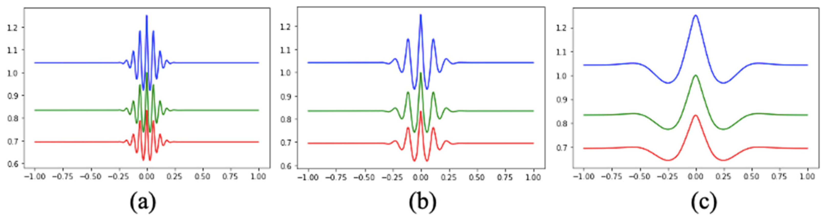
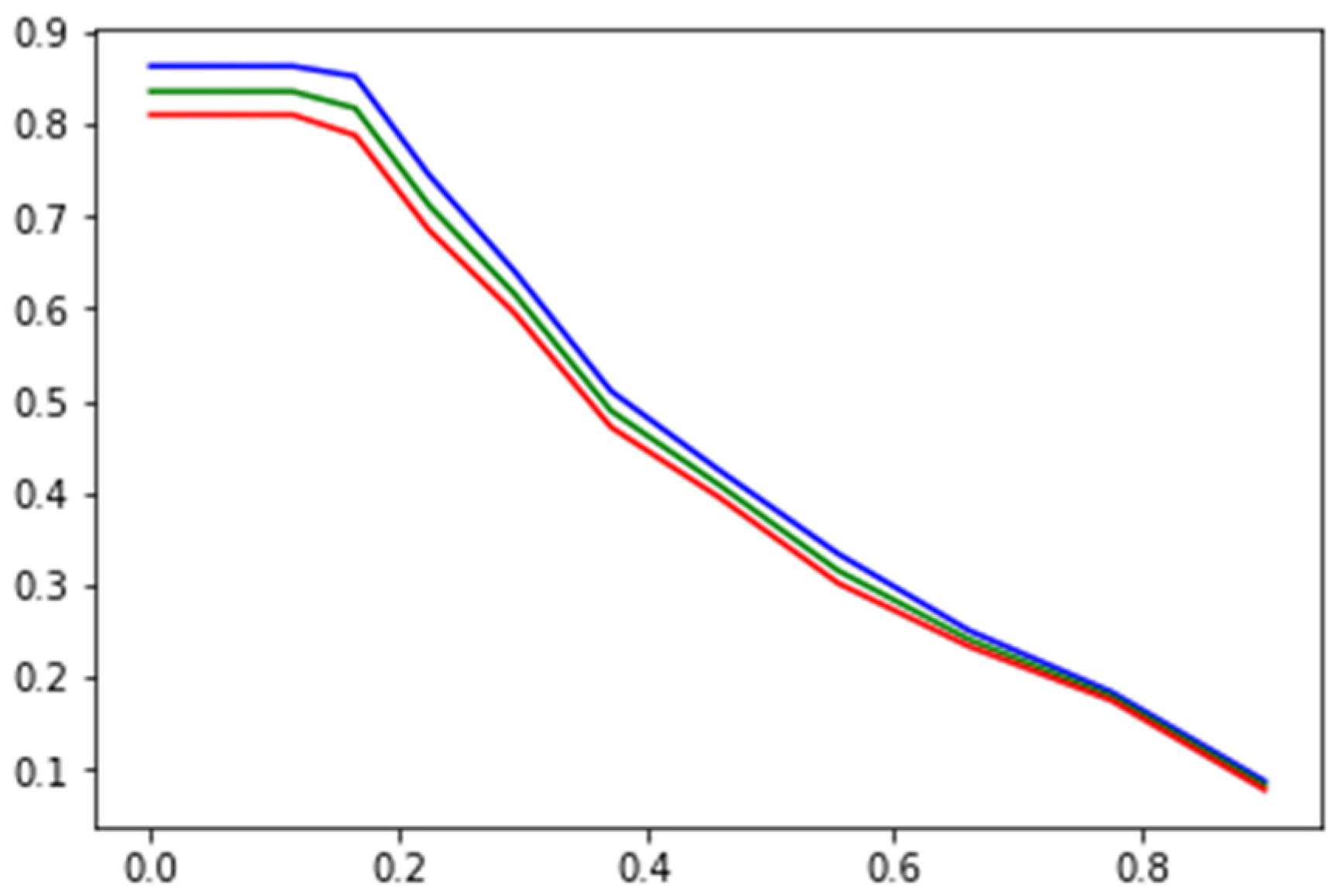
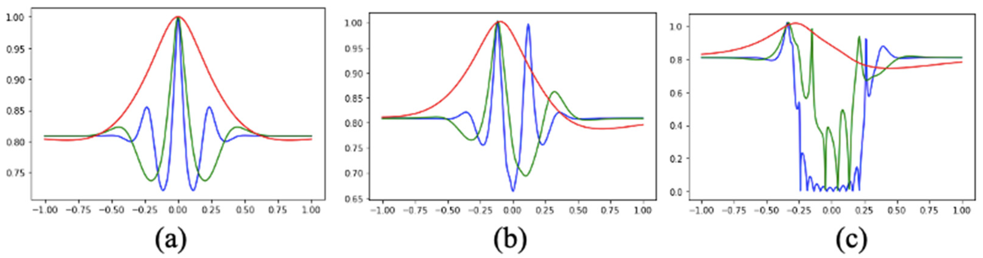
It was shown that there are oscillations of nanoparticle concentrations across the channel when the magnetic field is absent. These oscillations attenuate with time;

4.

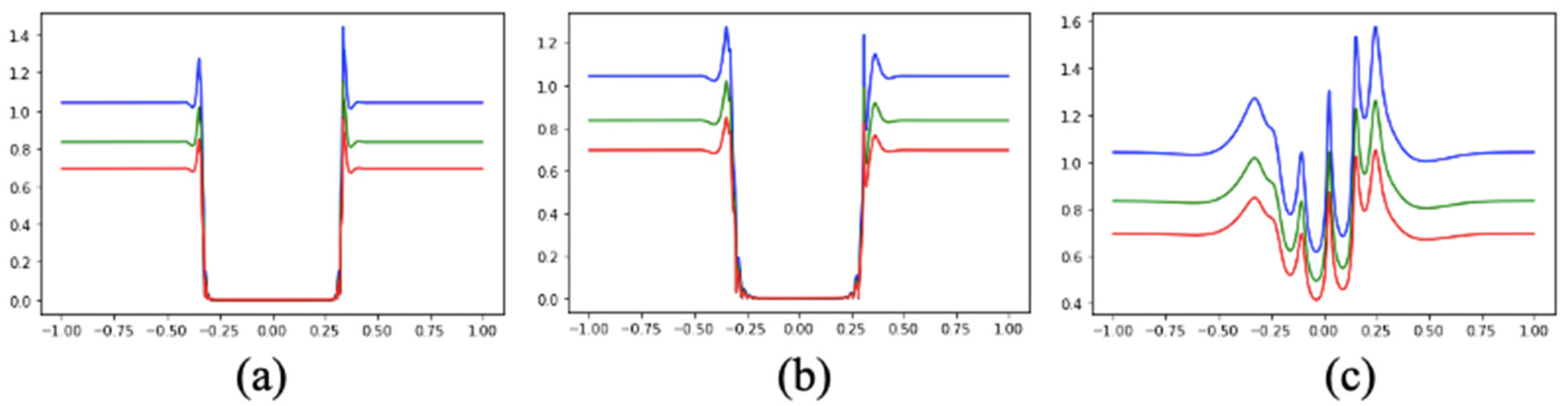
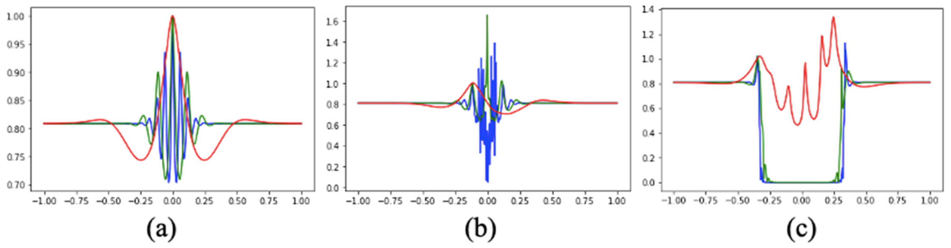
It was shown that nanoparticle concentrations become irregular oscillation under a weak magnetic field. The concentration in the turbulent part of the flow becomes almost zero in a strong magnetic field.

There are several physical consequences of the present study:

-

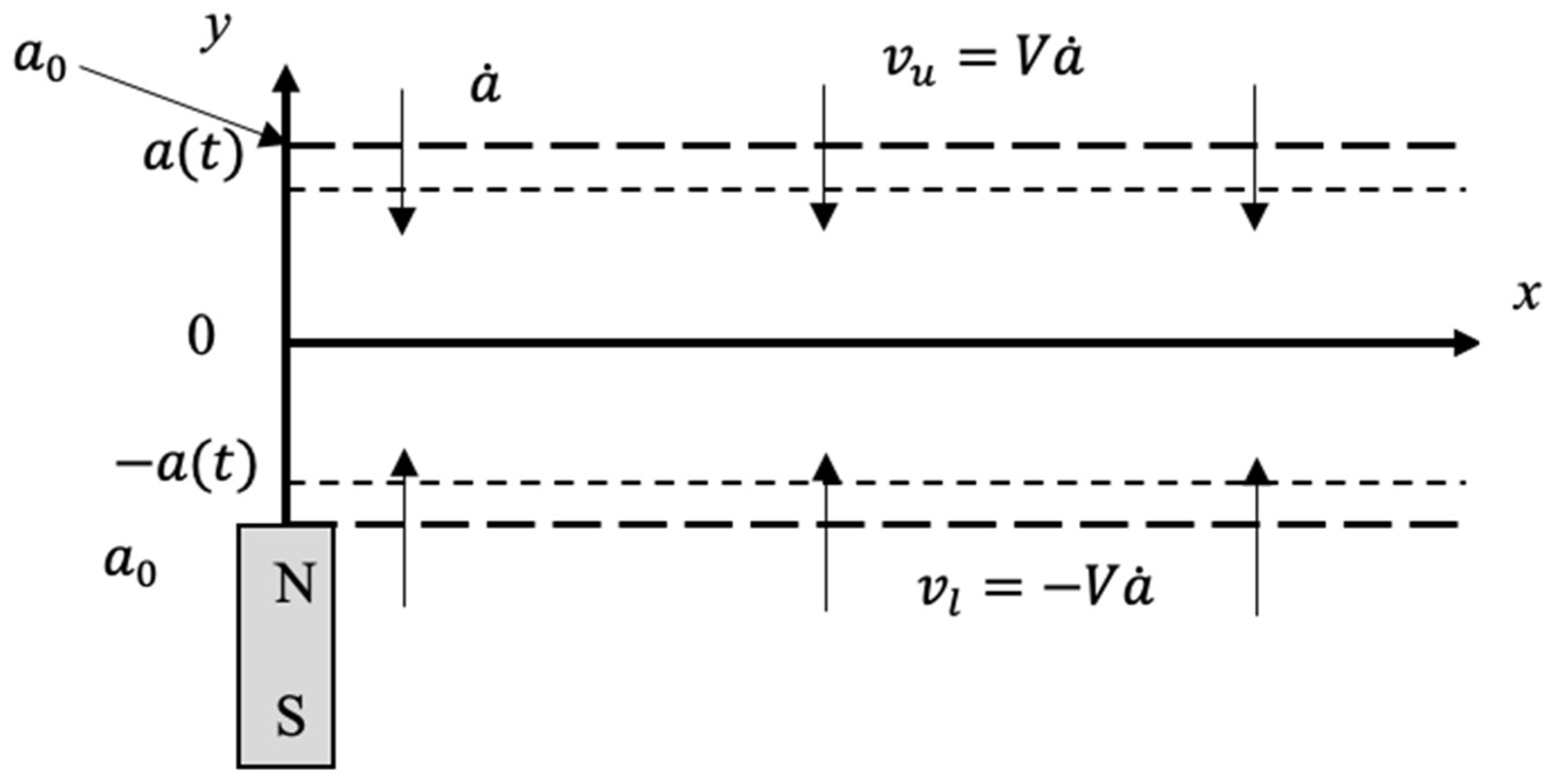
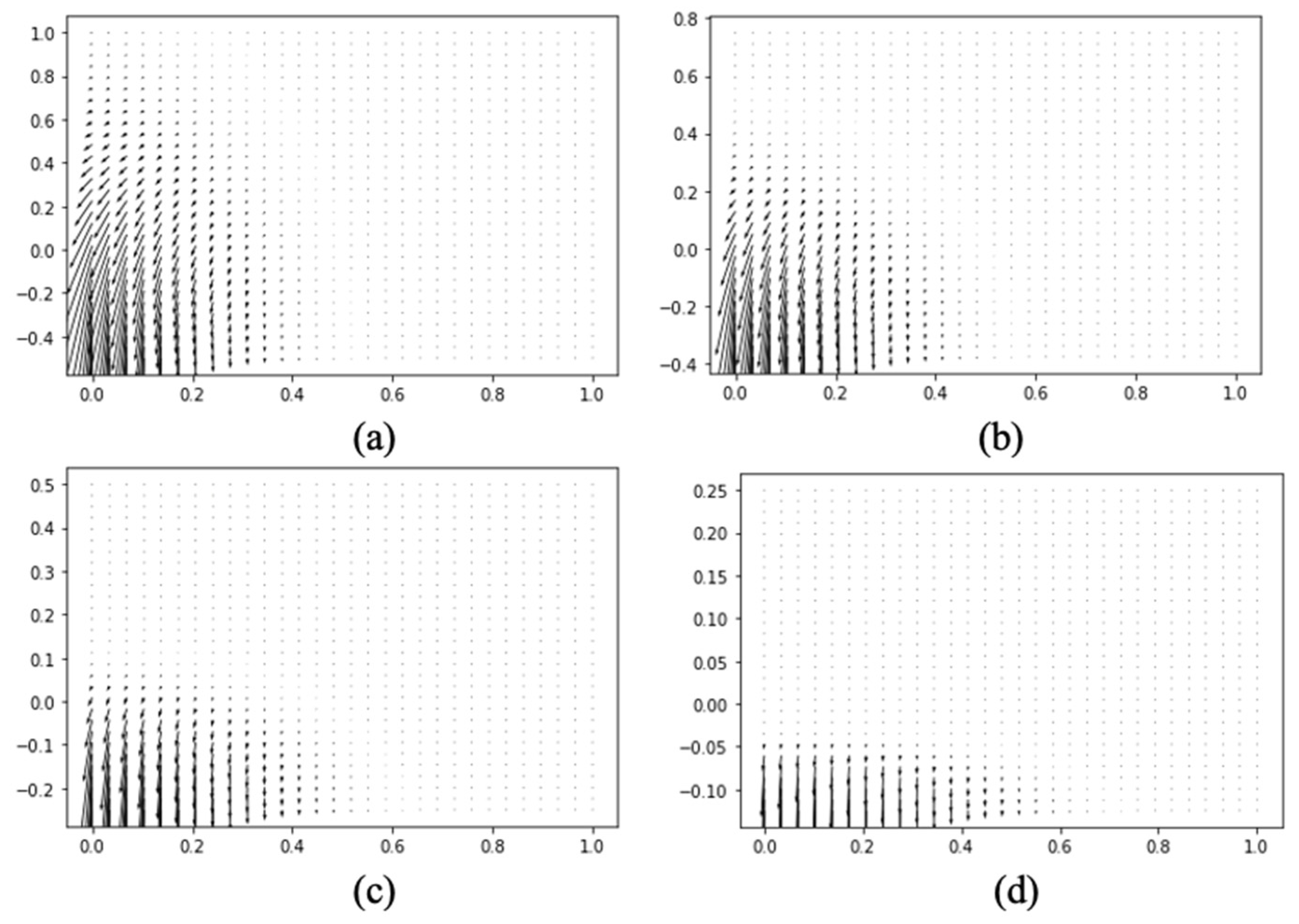
Any flow configuration shown in Figure 1 becomes partially unsteady when the channel is squeezed: the unstable flow occupies the central part of the channel, and stable layers are close to the walls.

-

When the channel is stretching, the whole flow is unsteady and there is no stable layer.

-

If there is nanofluid in the flow, then the nanoparticle concentration inside the unsteady zone can be extremely (practically down to zero) decreased if a magnetic field of enough magnitude (about 1 T) is applied. This is the purification effect that was the goal of the paper.

-

The value of the squeezing rate is essential for the presence of the purification effect: too fast squeezing destroys the purification abilities even if the magnetic field is strong enough.

References

1. Alfven, H. Existence of electromagnetic-hydrodynamic waves. Nature 1942, 150, 405–406. [Google Scholar] [CrossRef]
2. Hussain, Z.; Zeesahan, R.; Shahzad, M.; Ali, M.; Sultan, F.; Anter, A.M.; Zhang, H.; Khan, N. An optimised stability model for the magnetohydrodynamic fluid. Pramana 2021, 95, 27. [Google Scholar] [CrossRef]
3. Hussain, Z.; Ali, M.; Shahzad, M.; Sultan, F. Optimized wave perturbation for the linear instability of magnetohydrodynamics in plane Poiseuille flow. Pramana 2020, 94, 49. [Google Scholar] [CrossRef]
4. Hussain, Z.; Hussain, S.; Kong, T. Instability of MHD Couette flow of an electrically conducting fluid. AIP Adv. 2018, 8, 105209. [Google Scholar] [CrossRef]
5. Hussain, Z.; Zuev, S.; Kabobel, A.; Ali, M.; Sultan, F.; Shahzad, M. MHD instability of two fluids between parallel plates. Appl. Nanosci. 2020, 10, 5211–5218. [Google Scholar] [CrossRef]
6. Dalkılıç, A.S.; Yalçın, G.; Küçükyıldırım, B.O.; Öztuna, S.; Eker, A.A.; Jumpholkul, C.; Nakkaew, S.; Wongwises, S. Experimental study on the thermal conductivity of water-based CNT-SiO2 hybrid nanofluids. Int. Commun. Heat Mass Transf. 2018, 99, 18–25. [Google Scholar] [CrossRef]
7. Anisur, R.; Xu, W.; Li, K.; Dou, H.-S.; Khoo, B.C.; Mao, J. Influence of Magnetic Force on the Flow Stability in a Rectangular duct. Feb. Adv. Appl. Math. Mech. 2019, 11, 24–37. [Google Scholar] [CrossRef]
8. Hussain, Z.; Abbasi, A.Z.; Ahmad, R.; Bukhari, H.; Shahzad, M.; Sultan, F.; Ali, M. Vibrio cholerae dynamics in drinking water: Mathematical and statistical analysis. Appl. Nanosci. 2020, 10, 4519–4522. [Google Scholar] [CrossRef]
9. Zainal, N.; Nazar, R.; Naganthran, K.; Pop, I. Unsteady MHD mixed convection flow in hybrid nanofluid at three-dimensional stagnation point. Mathematics 2021, 9, 549. [Google Scholar] [CrossRef]
10. Zainal, N.A.; Nazar, R.; Naganthran, K.; Pop, I. Unsteady MHD stagnation point flow induced by exponentially permeable stretching/shrinking sheet of hybrid nanofluid. Eng. Sci. Technol. 2021, 24, 1201–1210. [Google Scholar] [CrossRef]
11. Sharma, K.; Kumar, S.; Narwal, A.; Mebarek-Oudina, F.; Animasaun, I.L. Convective MHD Fluid flow over Stretchable Rotating Disks with Dufour and Soret Effects. Int. J. Appl. Comput. Math. 2022, 8, 159. [Google Scholar] [CrossRef]
12. Kumar, S.; Sharma, K. Mathematical modeling of MHD flow and radiative heat transfer past a moving porous rotating disk with Hall effect. Multidiscip. Model. Mater. Struct. 2022, 18, 445–458. [Google Scholar] [CrossRef]
13. Hussain, Z.; Khan, N.; Gul, T.; Ali, M.; Shahzad, M.; Sultan, F. Instability of magneto hydro dynamics Couette flow for electrically conducting fluid through porous media. Appl. Nanosci. 2020, 10, 5125–5134. [Google Scholar] [CrossRef]
14. Downey, J.P.; Pojman, J.A. Polymer Research in Microgravity: Polymerization and Processing; American Chemical Society: Washington, DC, USA, 2001. [Google Scholar]
15. Jing, D.; Hu, Y.; Liu, M.; Wei, J.; Guo, L. Preparation of highly dispersed nanofluid and CFD study of its utilization in a concentrating PV/T system. Sol. Energy 2015, 112, 30–40. [Google Scholar] [CrossRef]
16. Kandelousi, M.S. Effect of spatially variable magnetic field on ferrofluid flow and heat transfer considering constant heat flux boundary condition. Eur. Phys. J. Plus 2014, 129, 248. [Google Scholar] [CrossRef]
17. Hussanan, A.; Khan, I.; Hashim, H.; Mohamed, M.K.A.; Ishak, N.; Sarif, N.M.; Salleh, M.Z. Unsteady MHD flow of some nanofluids past an accelerated vertical plate embedded in a porous medium. J. Teknol. 2016, 78, 121–126. [Google Scholar] [CrossRef]
18. Atkins, P.W.; De Paula, J.; Keeler, J. Atkins’ Physical Chemistry, 11th ed.; Oxford University Press: Oxford, UK, 2018; ISBN 978-0-19-876986-6. [Google Scholar]
19. Landau, L.D.; Lifshitz, E.M. Fluid Mechanics, 2nd ed.; Pergamon Press: Oxford, UK, 1987; 539p. [Google Scholar]
20. Griffiths, D.J. Introduction to Electrodynamics, 4th ed.; Cambridge University Press: Cambridge, UK, 2017; ISBN 978-1-108-42041-9. [Google Scholar] [CrossRef]
21. Babichev, A.P.; Babushkina, N.A.; Bratkovskii, A.M. Physical Values; Energoatomizdat: Moscow, Russia, 1991; pp. 123, 124, 370, 376. (In Russian) [Google Scholar]
22. Sobamowo, M.G.; Akinshilo, A.T. On the analysis of squeezing flow of nanofluid between two parallel plates under the influence of magnetic field. Alex. Eng. J. 2018, 57, 1413–1423. [Google Scholar] [CrossRef]
23. Kandasamy, R.; Zailani, N.A.B.M.; Jaafar, F.N.B. Impact of nanoparticle volume fraction on squeezed MHD water based Cu, Al2O3 and SWCNTs flow over a porous sensor surface. St. Petersb. Polytech. Univ. J. Phys. Math. 2017, 3, 308–321. [Google Scholar]
24. Dawar, A.; Shah, Z.; Khan, W.; Idrees, M.; Islam, S. Unsteady squeezing flow of magnetohydrodynamic carbon nanotube nanofluid in rotating channels with entropy generation and viscous dissipation. Adv. Mech. Eng. 2019, 11, 1687814018823100. [Google Scholar] [CrossRef]
Figure 1. Schematic vision of the channel and flow.
Symmetry 14 01728 g001
Figure 2. Magnetic field configurations for start squeezing (a), ¼ squeezing stroke (b), ½ squeezing stroke (c), and ¾ squeezing stroke (d).
Symmetry 14 01728 g002
Figure 3. Relative concentration of nanoparticles versus vertical position without a magnetic field, at t = 1 s (a), 10 s (b), and 18 s (c): reduced conc. (blue), standard conc. (green), increased conc. (red).
Symmetry 14 01728 g003
Figure 4. Relative concentration of nanoparticles versus vertical position under the 0.6 T magnetic field, at t = 1 s (a), 10 s (b), and 18 s (c): reduced conc. (blue), standard conc. (green), increased conc. (red).
Symmetry 14 01728 g004
Figure 5. Relative concentration of nanoparticles versus vertical position under the 0.9 T magnetic field, at t = 1 s (a), 10 s (b), and 18 s (c): reduced conc. (blue), standard conc. (green), increased conc. (red).
Symmetry 14 01728 g005
Figure 6. Relative concentration of nanoparticles versus magnetic field magnitude at t = 1 s: reduced conc. (blue), standard conc. (green), increased conc. (red).
Symmetry 14 01728 g006
Figure 7. Relative concentrations of nanoparticles versus vertical position under 0 T (a), 0.6 T (b), and 0.9 T (c) magnetic fields with a double squeezing rate, at t = 0.5 s (blue), 5 s (green), and 9 s (red).
Symmetry 14 01728 g007
Figure 8. Relative concentrations of nanoparticles versus vertical position under 0 T (a), 0.6 T (b), and 0.9 T (c) magnetic fields with a half squeezing rate, at t = 2 s (blue), 20 s (green), and 36 s (red).
Symmetry 14 01728 g008
Publisher’s Note: MDPI stays neutral with regard to jurisdictional claims in published maps and institutional affiliations.