
Theoretical Survey of Time-Dependent Micropolar Nanofluid Flow over a Linear Curved Stretching Surface


Abstract
:1. Introduction
2. Materials and Methods
- Unsteady flow;
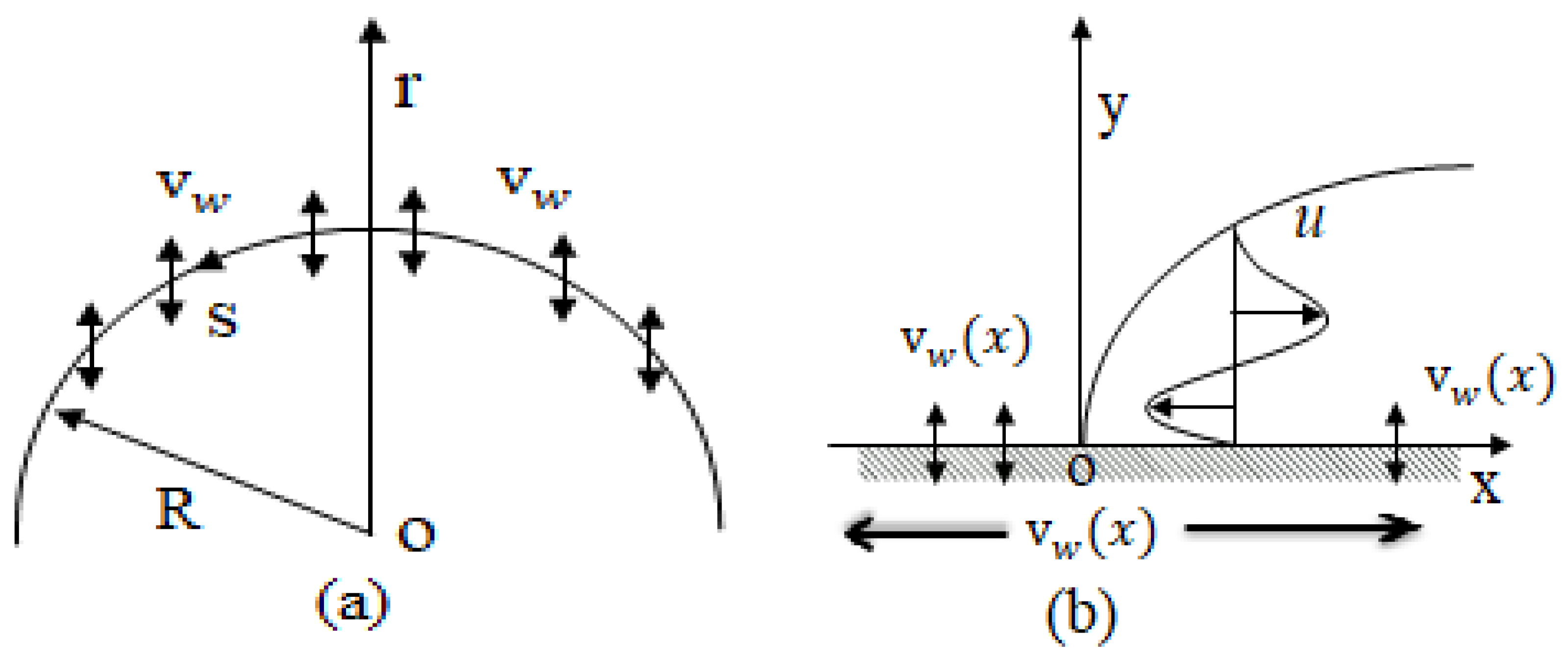
- Stretching curved surface;
- Micropolar fluid flow;
- Non-linear radiation;
- Thermal slip and velocity slip.
3. Numerical Procedure
4. Results and Discussion
5. Final Remarks
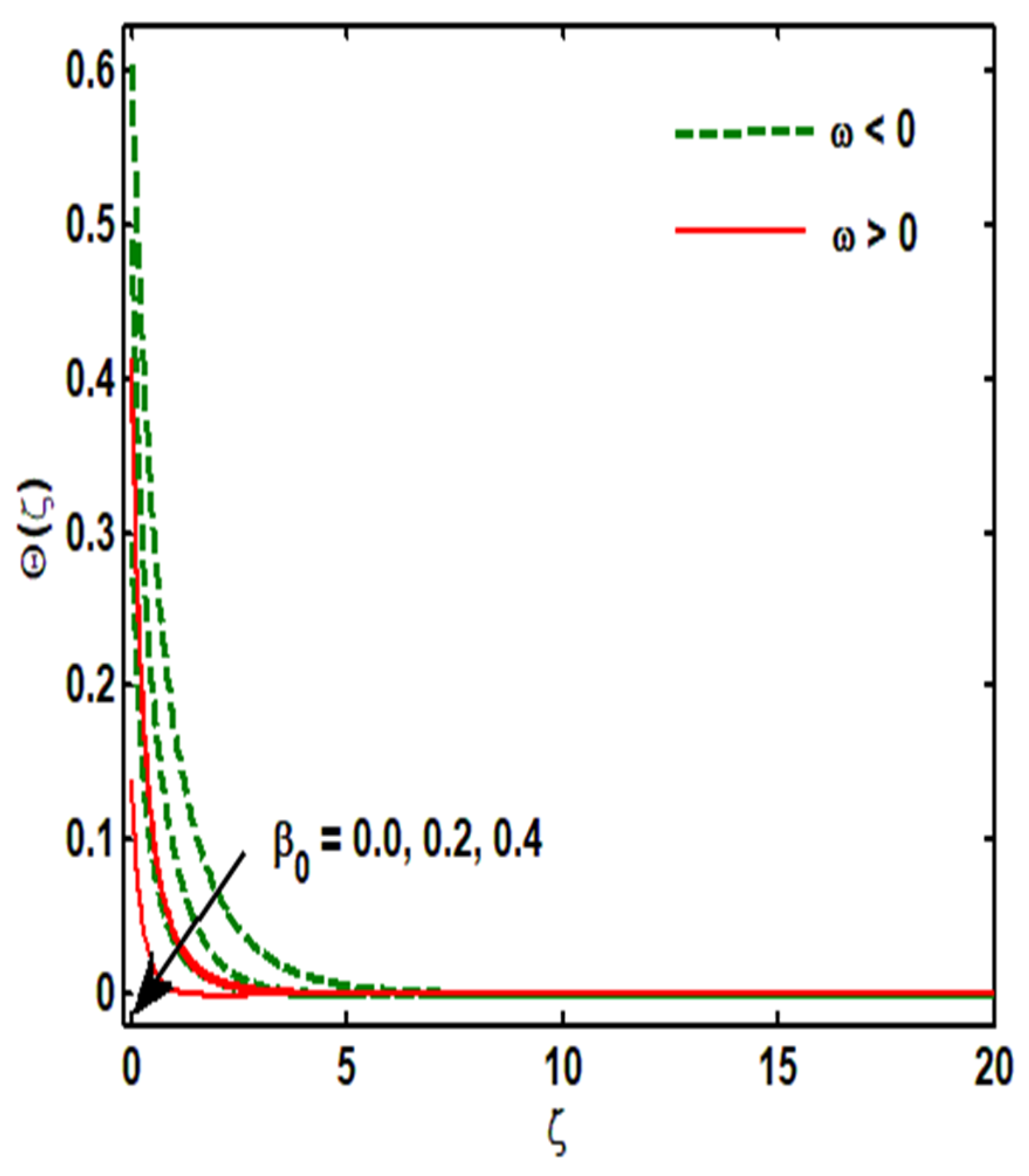
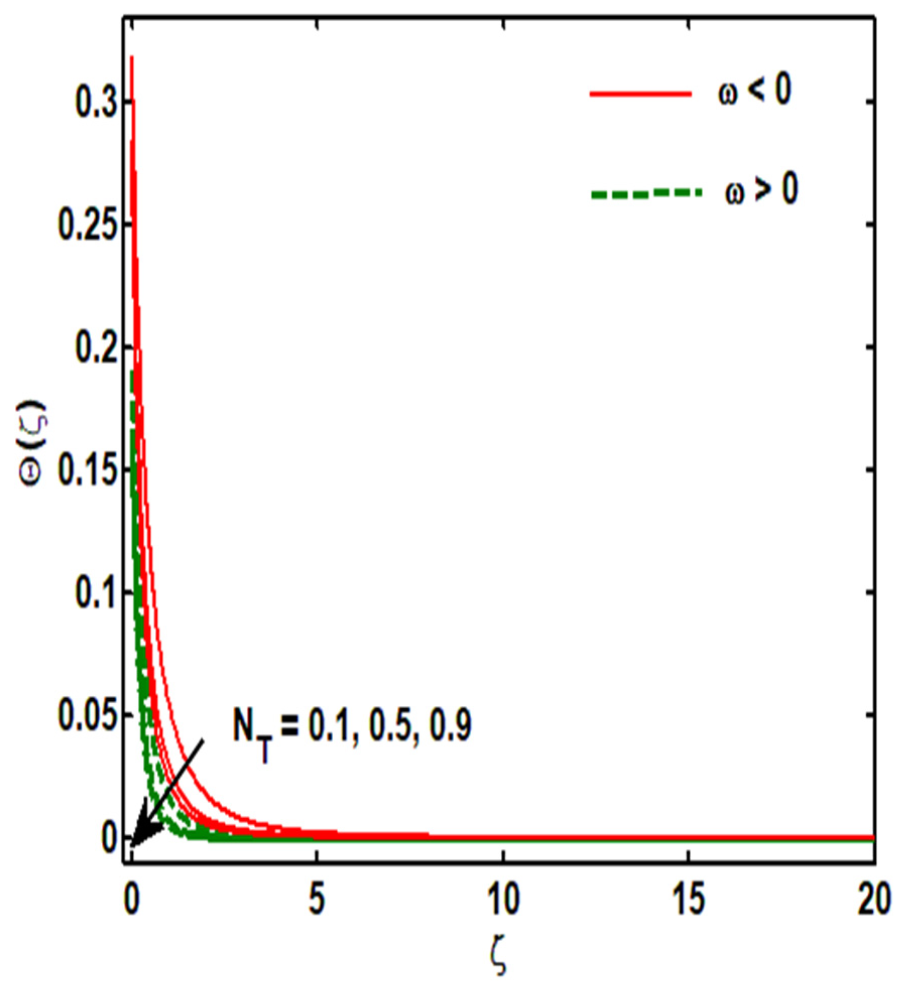
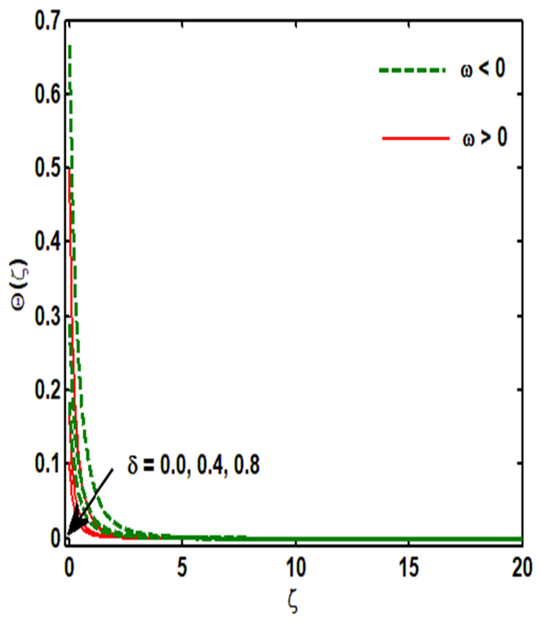
- In terms of the values of , , and , a weak concentration enables greater values in comparison to a strong concentration .
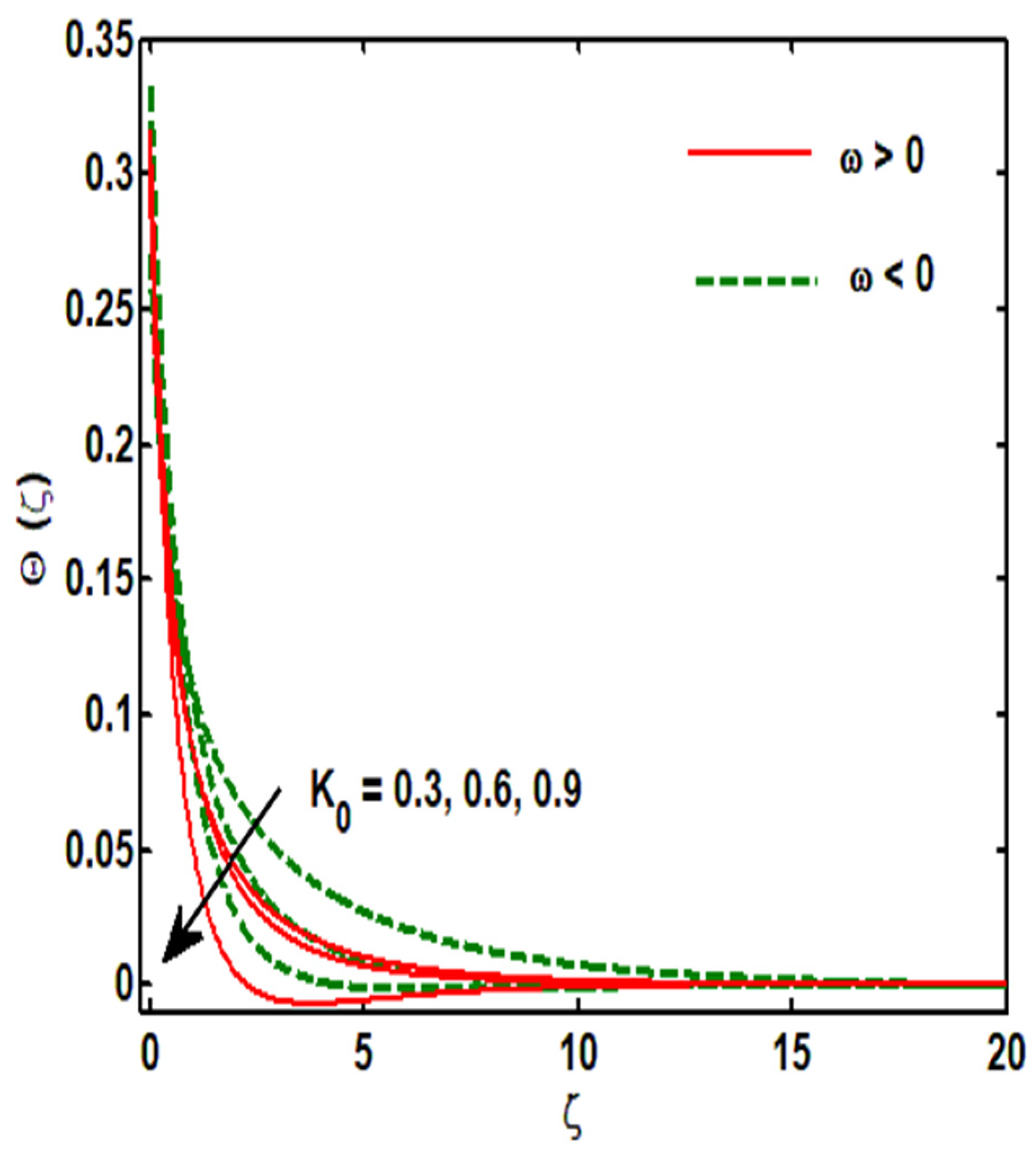
- The temperature profile achieves greater values near the surface in the case of as compared to .
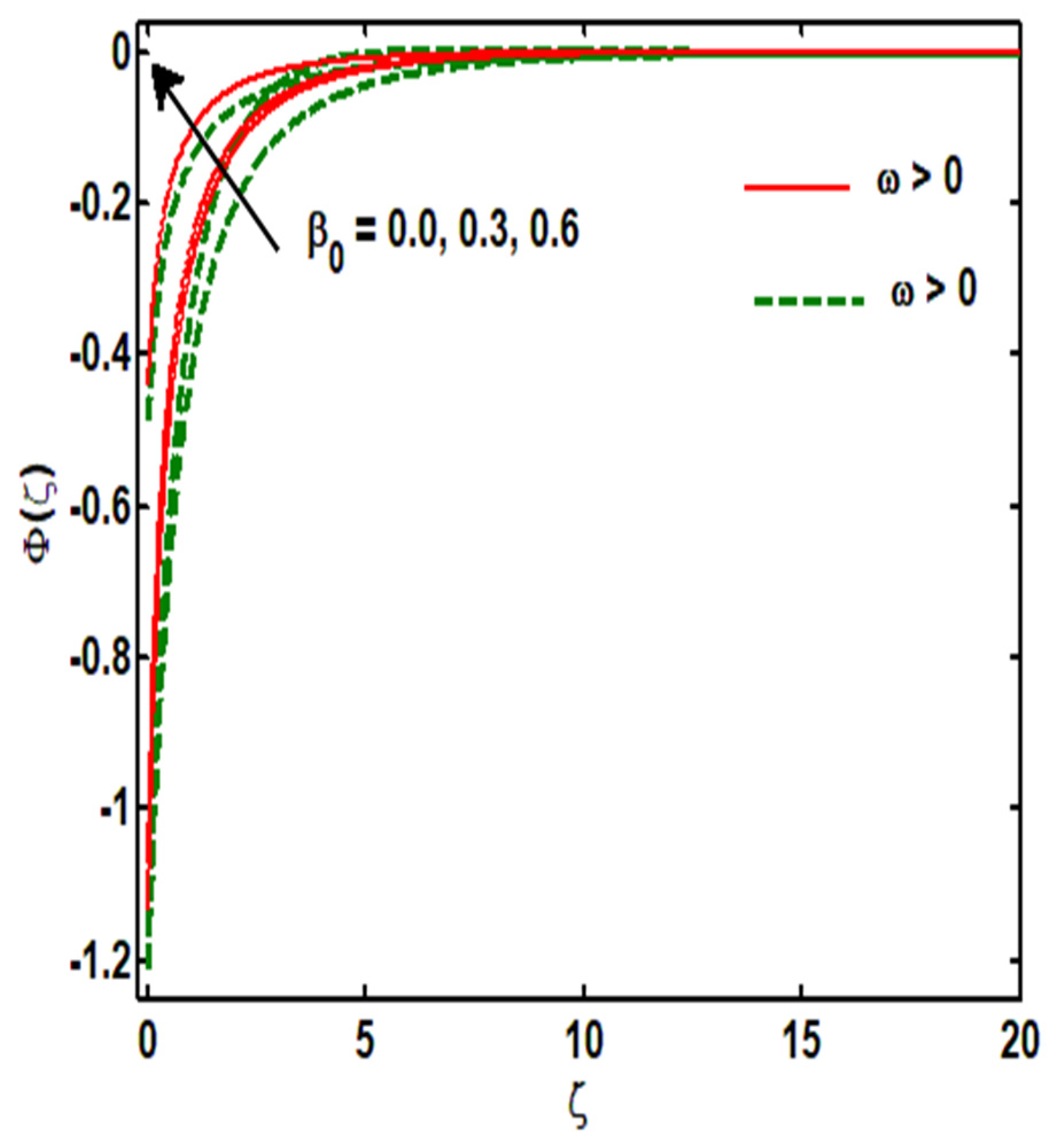
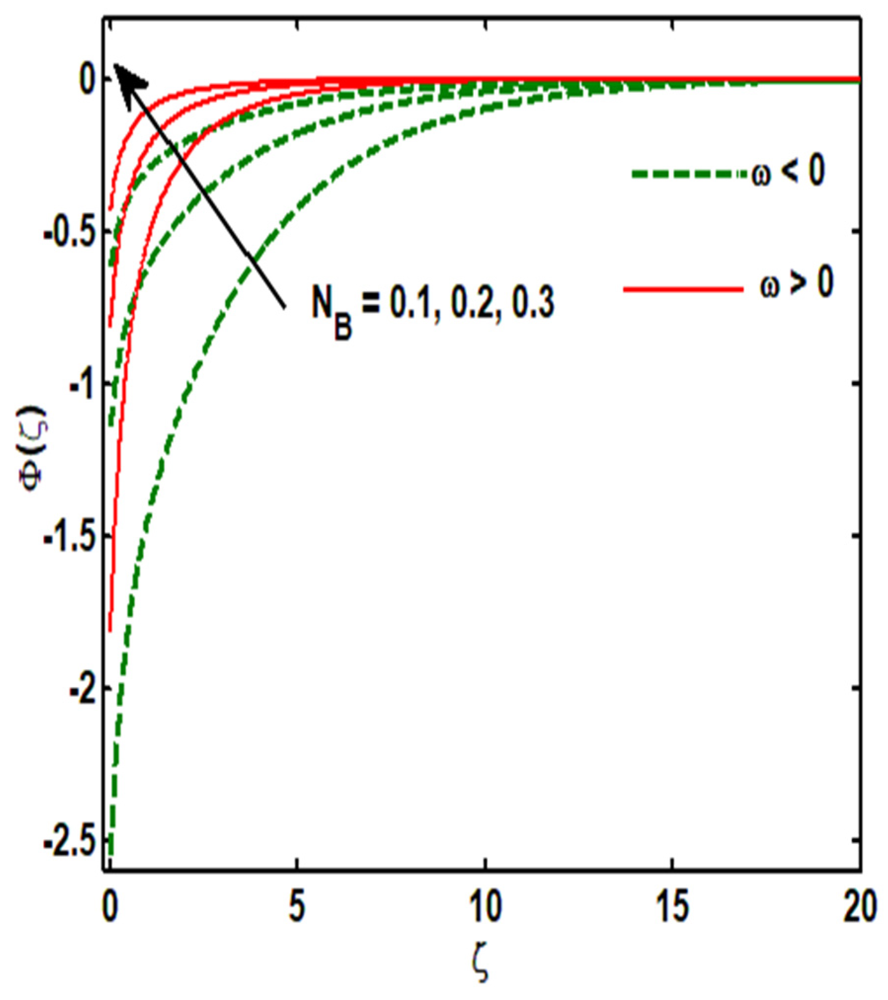
- Surprisingly, the concentration profile achieves greater values near the surface in the case of as compared to due to increments in the and .
- The unsteadiness parameter increases, which resists increases in the Nusselt number in a strong concentration but declines in a weak concentration .
- The thermophoresis parameter increases as the Nusselt number increases because the small number of nanoparticles enhances the heat transfer rate.
- The higher value of the unsteadiness parameter , the lower the temperature profile for the cases of both suction and injection.
Author Contributions
Funding
Institutional Review Board Statement
Informed Consent Statement
Data Availability Statement
Acknowledgments
Conflicts of Interest
Nomenclature
| (1) | Non-dimensional parameter |
| (1) | Reynolds number |
| (1) | Stretching parameter |
| Angular velocity components | |
| Velocity components | |
| (1) | Curvature parameter |
| Velocity vector r-direction | |
| Sherwood number | |
| Thermophoresis parameter | |
| (1) | Microgyration |
| (1) | Stretching parameter |
| Thermal diffusivity | |
| T (K) | Temperature |
| Wall temperature | |
| (1) | Stretching parameter |
| (1) | Micropolar parameter |
| Vertex viscosity | |
| Heat capacity of fluid | |
| Arc length | |
| (1) | Brownian motion parameter |
| (pa) | Wall shear stress |
| Wall temperature | |
| (1) | Prandtl number |
| (m) | Radius of curvature |
| Fluid density | |
| Ambient temperature | |
| Dynamic viscosity | |
| Ambient temperature | |
| (1) | Velocity slip |
References
- Choi, S.U.; Eastman, J.A. Enhancing Thermal Conductivity of Fluids with Nanoparticles (No. ANL/MSD/CP-84938; CONF-951135-29); Argonne National Lab.: Lemont, IL, USA, 1995. [Google Scholar]
- Masuda, H.; Ebata, A.; Teramae, K. Alteration of thermal conductivity and viscosity of liquid by dispersing ultra-fine particles. Dispersion of Al2O3, SiO2 and TiO2 ultra-fine particles. Netsu Bussei 1993, 7, 227–233. [Google Scholar] [CrossRef]
- Yu, W.; Mittra, R. A conformal finite difference time domain technique for modeling curved dielectric surfaces. IEEE Microw. Wirel. Compon. Lett. 2001, 11, 25–27. [Google Scholar] [CrossRef]
- Nadeem, S.; Lee, C. Boundary layer flow of nanofluid over an exponentially stretching surface. Nanoscale Res. Lett. 2012, 7, 94. [Google Scholar] [CrossRef] [PubMed] [Green Version]
- Nadeem, S.; Maraj, E. The mathematical analysis for peristaltic flow of hyperbolic tangent fluid in a curved channel. Commun. Theor. Phys. 2013, 59, 729–736. [Google Scholar] [CrossRef]
- Malvandi, A.; Hedayati, F.; Nobari, M.R.H. An HAM analysis of stagnation-point flow of a nanofluid over a porous stretching sheet with heat generation. J. Appl. Fluid Mech. 2014, 7, 135–145. [Google Scholar]
- Saleem, S.; Nadeem, S.; Awais, M. Time-dependent second-order viscoelastic fluid flow on rotating cone with heat generation and chemical reaction. J. Aerosp. Eng. 2016, 29, 4. [Google Scholar] [CrossRef]
- Nadeem, S.; Abbas, N. Effects of MHD on modified nanofluid model with variable viscosity in a porous medium. In Nanofluid Flow in Porous Media; IntechOpen: London, UK, 2019; pp. 109–117. [Google Scholar] [CrossRef] [Green Version]
- Hosseinzadeh, K.; Mardani, M.R.; Salehi, S.; Paikar, M.; Waqas, M.; Ganji, D.D. Entropy generation of three-dimensional Bödewadt flow of water and hexanol base fluid suspended by Fe3O4 and MoS2 hybrid nanoparticles. Pramana 2021, 95, 57. [Google Scholar] [CrossRef]
- Hosseinzadeh, K.; Roghani, S.; Mogharrebi, A.R.; Asadi, A.; Ganji, D.D. Optimization of hybrid nanoparticles with mixture fluid flow in an octagonal porous medium by effect of radiation and magnetic field. J. Therm. Anal. 2021, 143, 1413–1424. [Google Scholar] [CrossRef]
- Abbas, N.; Shatanawi, W. Heat and mass transfer of micropolar-casson nanofluid over vertical variable stretching riga sheet. Energies 2022, 15, 4945. [Google Scholar] [CrossRef]
- Eringen, A.C. Theory of micropolar fluids. J. Math. Mech. 1966, 16, 1–18. [Google Scholar] [CrossRef]
- Ahmadi, G. Self-similar solution of imcompressible micropolar boundary layer flow over a semi-infinite plate. Int. J. Eng. Sci. 1976, 14, 639–646. [Google Scholar] [CrossRef]
- Gorla, R.S.R. Mixed convection in a micropolar fluid from a vertical surface with uniform heat flux. Int. J. Eng. Sci. 1992, 30, 349–358. [Google Scholar] [CrossRef]
- Kelson, N.; Desseaux, A. Effect of surface conditions on flow of a micropolar fluid driven by a porous stretching sheet. Int. J. Eng. Sci. 2001, 39, 1881–1897. [Google Scholar] [CrossRef]
- Bhargava, R.; Kumar, L.; Takhar, H. Finite element solution of mixed convection micropolar flow driven by a porous stretching sheet. Int. J. Eng. Sci. 2003, 41, 2161–2178. [Google Scholar] [CrossRef]
- Qasim, M.; Khan, I.; Shafie, S. Heat transfer in a micropolar fluid over a stretching sheet with newtonian heating. PLoS ONE 2013, 8, e59393. [Google Scholar] [CrossRef] [PubMed] [Green Version]
- Ishak, A.; Nazar, R.; Pop, I. Magnetohydrodynamic (MHD) flow of a micropolar fluid towards a stagnation point on a vertical surface. Comput. Math. Appl. 2008, 56, 3188–3194. [Google Scholar] [CrossRef] [Green Version]
- Nadeem, S.; Abbas, N. On both MHD and slip effect in micropolar hybrid nanofluid past a circular cylinder under stagnation point region. Can. J. Phys. 2018, 97, 392–399. [Google Scholar] [CrossRef]
- Nadeem, S.; Malik, M.Y.; Abbas, N. Heat transfer of three-dimensional micropolar fluid on a Riga plate. Can. J. Phys. 2019, 98, 32–38. [Google Scholar] [CrossRef]
- Abbas, N.; Rehman, K.U.; Shatanawi, W.; Al-Eid, A.A. Theoretical study of non-Newtonian micropolar nanofluid flow over an ex-ponentially stretching surface with free stream velocity. Adv. Mech. Eng. 2022, 14, 16878132221107790. [Google Scholar] [CrossRef]
- Fuzhang, W.; Anwar, M.I.; Ali, M.; El-Shafay, A.S.; Abbas, N.; Ali, R. Inspections of unsteady micropolar nanofluid model over ex-ponentially stretching curved surface with chemical reaction. Waves Random Complex Media 2022, 1–22. [Google Scholar] [CrossRef]
- Saffman, P.G. On the boundary condition at the surface of a porous medium. Stud. Appl. Math. 1971, 50, 93–101. [Google Scholar] [CrossRef]
- Chellam, S.; Wiesner, M.R.; Dawson, C. Slip at a uniformly porous boundary: Effect on fluid flow and mass transfer. J. Eng. Math. 1992, 26, 481–492. [Google Scholar] [CrossRef]
- Sharma, P.K.; Chaudhary, R.C. Effect of variable suction on transient free convection viscous incompressible flow past a vertical plate with periodic temperature variations in slip-flow regime. Emir. J. Eng. Res. 2003, 8, 33–38. [Google Scholar]
- Sharma, P.K. Fluctuating thermal and mass diffusion on unsteady free convection flow past a vertical plate in slip-flow regime. Lat. Am. Appl. Res. 2005, 35, 313–319. [Google Scholar]
- Ibrahim, W.; Shankar, B. MHD boundary layer flow and heat transfer of a nanofluid past a permeable stretching sheet with velocity, thermal and solutal slip boundary conditions. Comput. Fluids 2013, 75, 1–10. [Google Scholar] [CrossRef]
- Xinhui, S.; Liancun, Z.; Xuehui, C.; Xinxin, Z.; Limei, C.; Min, L. The effects of slip velocity on a micropolar fluid through a porous channel with expanding or contracting walls. Comput. Methods Biomech. Biomed. Eng. 2014, 17, 423–432. [Google Scholar] [CrossRef] [PubMed]
- Abbas, N.; Rehman, K.U.; Shatanawi, W.; Malik, M. Numerical study of heat transfer in hybrid nanofluid flow over permeable nonlinear stretching curved surface with thermal slip. Int. Commun. Heat Mass Transf. 2022, 135, 106107. [Google Scholar] [CrossRef]
- Abbas, N.; Nadeem, S.; Khan, M.N. Numerical analysis of unsteady magnetized micropolar fluid flow over a curved surface. J. Therm. Anal. 2021, 147, 6449–6459. [Google Scholar] [CrossRef]
- Amjad, M.; Zehra, I.; Nadeem, S.; Abbas, N. Thermal analysis of Casson micropolar nanofluid flow over a permeable curved stretching surface under the stagnation region. J. Therm. Anal. 2021, 143, 2485–2497. [Google Scholar] [CrossRef]
- Nadeem, S.; Abbas, N.; Malik, M. Inspection of hybrid based nanofluid flow over a curved surface. Comput. Methods Programs Biomed. 2020, 189, 105193. [Google Scholar] [CrossRef]
- Abbas, N.; Shatanawi, W.; Abodayeh, K. Computational Analysis of MHD Nonlinear Radiation Casson Hybrid Nanofluid Flow at Vertical Stretching Sheet. Symmetry 2022, 14, 1494. [Google Scholar] [CrossRef]
- Abbas, N.; Nadeem, S.; Saleem, A. Computational analysis of water based Cu-Al2O3/H2O flow over a vertical wedge. Adv. Mech. Eng. 2020, 12, 1687814020968322. [Google Scholar] [CrossRef]
- Ahmad, S.; Khan, Z.H. Numerical solution of micropolar fluid flow with heat transfer by finite difference method. Int. J. Mod. Phys. B 2022, 36, 2250037. [Google Scholar] [CrossRef]
- Noghrehabadi, A.; Pourrajab, R.; Ghalambaz, M. Effect of partial slip boundary condition on the flow and heat transfer of nanofluids past stretching sheet prescribed constant wall temperature. Int. J. Therm. Sci. 2012, 54, 253–261. [Google Scholar] [CrossRef]
- Sahoo, B.; Poncet, S. Flow and heat transfer of a third grade fluid past an exponentially stretching sheet with partial slip boundary condition. Int. J. Heat Mass Transf. 2011, 54, 5010–5019. [Google Scholar] [CrossRef] [Green Version]


| 0.10 | 0.5 | 0.5 | 0.5 | 0.5 | 0.5 | 0.4 | 0.4 | 0.4 | 0.4 | 1.2700 | 0.3774 | −0.6640 |
| 0.30 | 1.0252 | 1.6475 | −1.5880 | |||||||||
| 0.50 | 0.3034 | 1.8409 | −2.3542 | |||||||||
| 0.70 | 0.0525 | 2.2916 | −3.4971 | |||||||||
| 0.50 | 0.10 | 1.3240 | 1.5409 | −3.3542 | ||||||||
| 0.30 | 1.3170 | 1.5409 | −3.3542 | |||||||||
| 0.50 | 1.3034 | 1.5409 | −3.3542 | |||||||||
| 0.70 | 1.2840 | 1.5409 | −3.3542 | |||||||||
| 0.50 | 0.10 | 1.2245 | 1.5409 | −3.3542 | ||||||||
| 0.30 | 1.2862 | 1.5409 | −3.3542 | |||||||||
| 0.50 | 1.3034 | 1.5409 | −3.3542 | |||||||||
| 0.70 | 1.3137 | 1.5409 | −3.3542 | |||||||||
| 0.50 | 0.10 | 1.4242 | 1.3640 | −2.8175 | ||||||||
| 0.30 | 1.3583 | 1.4737 | −3.0859 | |||||||||
| 0.50 | 1.3034 | 1.5409 | −3.3542 | |||||||||
| 0.70 | 1.2569 | 1.5655 | −3.6225 | |||||||||
| 0.50 | 0.10 | 1.2831 | −0.7659 | −0.5922 | ||||||||
| 0.30 | 1.2956 | 1.6675 | −1.1999 | |||||||||
| 0.50 | 1.3296 | 1.8126 | −2.2200 | |||||||||
| 0.70 | 1.8271 | 2.2740 | 2.5751 | |||||||||
| 0.50 | 0.10 | 1.3156 | −0.8746 | −0.3638 | ||||||||
| 0.30 | 1.2361 | −1.2702 | −1.1912 | |||||||||
| 0.50 | 1.1296 | −1.5126 | −1.2200 | |||||||||
| 0.70 | 1.0426 | −2.4959 | −1.6223 | |||||||||
| 0.50 | 0.00 | 1.2849 | 2.1518 | −4.0259 | ||||||||
| 0.20 | 1.3074 | 1.8256 | −3.6167 | |||||||||
| 0.40 | 1.3296 | 1.5126 | −3.2200 | |||||||||
| 0.60 | 1.3514 | 1.2097 | −2.8323 | |||||||||
| 0.40 | 0.00 | 1.0927 | −1.4449 | −2.6394 | ||||||||
| 0.20 | 1.1381 | −1.6614 | −3.0333 | |||||||||
| 0.40 | 1.3296 | −1.8126 | −3.2200 | |||||||||
| 0.60 | 1.3370 | −2.0450 | −3.4929 | |||||||||
| 0.40 | 0.00 | 1.0863 | 0.9174 | −2.0755 | ||||||||
| 0.20 | 1.2045 | −1.3762 | −2.2529 | |||||||||
| 0.40 | 1.3296 | −1.5126 | −3.2200 | |||||||||
| 0.60 | 1.4658 | −2.0693 | −3.4202 | |||||||||
| 0.40 | 0.00 | 2.7467 | 1.5126 | −3.2200 | ||||||||
| 0.20 | 1.7981 | 1.5126 | −3.2200 | |||||||||
| 0.40 | 1.3296 | 1.5126 | −3.2200 | |||||||||
| 0.60 | 1.0529 | 1.5126 | −3.2200 |
| 0.10 | 0.5 | 0.5 | 0.5 | 0.5 | 0.5 | 0.4 | 0.4 | 0.4 | 0.4 | 1.2387 | −0.4436 | −0.4829 |
| 0.30 | 1.3774 | −0.5491 | −0.5038 | |||||||||
| 0.50 | 1.4413 | −1.0546 | −1.4398 | |||||||||
| 0.70 | 1.5472 | −1.1999 | −1.7156 | |||||||||
| 0.50 | 0.10 | 1.1634 | −1.0546 | −1.4398 | ||||||||
| 0.30 | 1.0559 | −1.0546 | −1.4398 | |||||||||
| 0.50 | 1.0413 | −1.0546 | −1.4398 | |||||||||
| 0.70 | 1.0206 | −1.0546 | −1.4398 | |||||||||
| 0.50 | 0.10 | 0.9572 | −1.0546 | −1.4398 | ||||||||
| 0.30 | 1.0226 | −1.0546 | −1.4398 | |||||||||
| 0.50 | 1.0413 | −1.0546 | −1.4398 | |||||||||
| 0.70 | 1.0526 | −1.0546 | −1.4398 | |||||||||
| 0.50 | 0.10 | 1.1131 | −0.9813 | −1.2598 | ||||||||
| 0.30 | 1.0630 | −1.0395 | −1.3798 | |||||||||
| 0.50 | 1.0215 | −1.0606 | −1.4998 | |||||||||
| 0.70 | 0.9862 | −1.0447 | −1.6198 | |||||||||
| 0.50 | 0.10 | 0.9124 | −2.2180 | −1.5941 | ||||||||
| 0.30 | 1.0343 | −1.3561 | −1.5290 | |||||||||
| 0.50 | 1.0413 | −1.0546 | −1.4398 | |||||||||
| 0.70 | 0.5037 | −22.9779 | 10.7449 | |||||||||
| 0.50 | 0.10 | 1.5078 | −1.9102 | −1.9608 | ||||||||
| 0.30 | 0.6701 | −1.3918 | −2.1640 | |||||||||
| 0.50 | 0.3413 | −1.0546 | −2.4398 | |||||||||
| 0.70 | 0.1856 | −1.0211 | −3.2148 | |||||||||
| 0.50 | 0.00 | 0.9768 | −1.0076 | −1.2888 | ||||||||
| 0.20 | 1.0094 | −1.0319 | −1.3616 | |||||||||
| 0.40 | 1.0413 | −1.0546 | −1.4398 | |||||||||
| 0.60 | 1.0727 | −1.0764 | −1.5233 | |||||||||
| 0.40 | 0.00 | 1.0273 | −1.0219 | −1.1099 | ||||||||
| 0.20 | 1.0362 | −1.0530 | −1.3134 | |||||||||
| 0.40 | 1.0413 | −1.0546 | −1.4398 | |||||||||
| 0.60 | 1.2837 | −1.0807 | −1.5794 | |||||||||
| 0.40 | 0.00 | 0.5517 | −1.0230 | −0.7457 | ||||||||
| 0.20 | 0.6602 | −1.0463 | −0.8614 | |||||||||
| 0.40 | 1.0413 | −1.0546 | −1.4398 | |||||||||
| 0.60 | 1.2326 | −1.0736 | −1.6826 | |||||||||
| 0.40 | 0.00 | 2.1024 | −1.0546 | −1.4398 | ||||||||
| 0.20 | 1.3965 | −1.0546 | −1.4398 | |||||||||
| 0.40 | 1.0413 | −1.0546 | −1.4398 | |||||||||
| 0.60 | 0.8296 | −1.0546 | −1.4398 |
| Sahoo and Do [33] | Nogrehabadi et al. [34] | Present Results | |
|---|---|---|---|
| 0.00 | 1.00112 | 1.00021 | 1.00001 |
| 0.10 | 0.87143 | 0.87204 | 0.871721 |
| 0.20 | 0.77491 | 0.77633 | 0.776014 |
| 0.30 | 0.69974 | 0.70152 | 0.700910 |
| 0.50 | 0.58912 | 0.59110 | 0.591021 |
| 1.00 | 0.42841 | 0.43011 | 0.430211 |
Publisher’s Note: MDPI stays neutral with regard to jurisdictional claims in published maps and institutional affiliations. |
© 2022 by the authors. Licensee MDPI, Basel, Switzerland. This article is an open access article distributed under the terms and conditions of the Creative Commons Attribution (CC BY) license (https://creativecommons.org/licenses/by/4.0/).
Share and Cite
Abbas, N.; Shatanawi, W. Theoretical Survey of Time-Dependent Micropolar Nanofluid Flow over a Linear Curved Stretching Surface. Symmetry 2022, 14, 1629. https://doi.org/10.3390/sym14081629
Abbas N, Shatanawi W. Theoretical Survey of Time-Dependent Micropolar Nanofluid Flow over a Linear Curved Stretching Surface. Symmetry. 2022; 14(8):1629. https://doi.org/10.3390/sym14081629
Chicago/Turabian StyleAbbas, Nadeem, and Wasfi Shatanawi. 2022. "Theoretical Survey of Time-Dependent Micropolar Nanofluid Flow over a Linear Curved Stretching Surface" Symmetry 14, no. 8: 1629. https://doi.org/10.3390/sym14081629