Research on the Stability of Anti-Slip Pile Support Structures for Railway Pile Slopes

Abstract

The accumulation slope is widely distributed in the mountainous area of China; this paper takes the slope of the Chengdu–Lanzhou Railway as the engineering background and analyzes the stability of the slope and the mechanical properties of the anti-slip pile under symmetrical train loads. First, the finite element software Midas GTS NX was used to analyze the effect of the slope after the anti-slip pile support and the stability of the slope at different pile spacings, pile row distances, and pile positions. Then, the finite element analysis results of the pile-side earth pressure and landslide thrust were compared with those of earth pressure theory, the standard method, and field-measured data. The results of this paper are as follows: (1) The anti-slip pile support increased the slope stability coefficient from 1.175 to 1.680. (2) The slope stability gradually decreased with increases in anti-slip pile spacing and pile row distance and rose first and then decreased with an increase in pile position. (3) The active earth pressure values behind the pile by Coulomb theory were slightly smaller than the finite element analysis result; the theoretical values of the passive pressure before the pile were much larger than the finite element analysis results. (4) The landslide thrust was calculated by the transfer coefficient method when the safety factor K = 1.00. The results of explicit method and implicit method were the same, which were 8–19% higher than the finite element simulation value; when the safety factor K = 1.35, the theoretical value of the explicit method was about three times the simulated value, and the theoretical value of the implicit method was about 2.3 times the simulated value. (5) The measured values verified that the simulated values had a certain degree of reliability, and the relative deviation between the two was 5–17%.

1. Introduction

In recent years, with the rapid advancement of infrastructure, China’s railway construction has made great achievements. At the same time, as trains usually travel at high speeds, the impact on the stability and mechanical properties of slopes is often greater, especially in hilly and mountainous areas, where they pass through high embankments, deep cuttings, and geologically complex areas, which can pose a threat to the safety of subsequent railway operations if not properly designed or constructed. Therefore, the stability of railway slopes has been paid more and more attention by the engineering community.

In the field of slope stability, scholars have conducted a lot of research and come up with some valuable conclusions. Zhang Zongzhan [1] analyzed the influence of different loading parameters on the stability of highway slopes based on the strength reduction method (SRM). Wei Meng et al. [2] studied the variation characteristics of the plastic zone, displacement, and the stability coefficient of a high embankment under geogrid reinforcement. Cheng Aiping et al. [3] first used the SRM to determine the slope stability coefficient, then obtained the landslide thrust by the unbalanced thrust method and proposed the reinforcement scheme of double-row anti-slip pile support. Jia Xingli et al. [4] studied the permanent displacement response law of a slope based on the combined analysis of the influencing factors (slope height, slope rate, rock inclination, and seismic parameters) of highway slope stability under seismic conditions. Fang Jingcheng et al. [5] used a finite element simulation to study the effects of the pile–soil stiffness ratio and pile position on slope stability and the pile body internal force. Rao Pingping et al. [6] and Wang Xiaofang et al. [7] studied the effects of slope stability coefficients and damage modes at different pile positions, pile spacings, pile lengths, and slope dimensions. Xu Hong et al. [8] and Wu Keliang et al. [9] analyzed the sensitivity of various influencing factors on slope stability based on orthogonal tests. Murat Olgun [10] studied slopes under seismic conditions and analyzed the effects of seismic horizontal acceleration, pore water pressure, soil shear strength, and slope geometry on slope stability. Jing Jing et al. [11] studied the variation characteristics of loess slope stability under different dry–wet cycle conditions. Karthik A. V. R. [12] analyzed the influencing factors of slope stability by the finite element method. It was found that slope stability was significantly affected by slope height, slope, bulk density, cohesion, and friction angle but little affected by the soil elastic modulus, Poisson’s ratio, the constitutive model, and the foundation soil distribution. Nilo Lemuel J [13] improved the Green–Ampt seepage equation and took a slope as an example to obtain the seepage depth and slope stability coefficient under the condition of rainfall. Susumu Nakajima [14] used the impact load test method to study the influence of earthquakes on slope stability and provide design ideas for slope anti-slip and rockfall protection. Zhuang, Y. [15] studied the effects of pile spacing, embankment height, vehicle load magnitude, and vehicle speed on the tension of a geogrid using numerical simulation. Zhang, B. [16] studied the calculation of slope stability coefficients for swelling soils under the combined influence of saturation and swelling. Guo, M.-Z. [17] studied the effects of dynamic parameters, seismic wave types, and weak rock formations on the dynamic responses of slopes using a model dynamic load test.

As can be seen from the above-mentioned scholars’ studies, most of them mainly focused on the influence of conventional loads on slope stability, mostly on single-row pile structures, with less research on double-row piles; there is less research on the influence of potential sliding surfaces under the roadbed and the relative positions of double-row anti-slip piles on slope stability, and most of the research is for highway slopes, with less research on railway slopes. The mechanical characteristics and safety requirements of railway slopes are different from those of highway slopes due to the different nature of loading, and the requirements are higher. However, the current railway design code only makes some principal provisions for anti-slip pile support structures and involves less content for the design of double-row pile support structures. Therefore, the study of double-row pile supports and their stability for railway accumulation slopes has important theoretical and practical engineering significance.

Therefore, in this paper, taking a railway accumulation layer slope as an example, Midas GTS NX finite element software was used to analyze the slope stability and the mechanical characteristics of the pile–soil interaction under different anti-slip pile conditions (pile spacings, row spacings, and pile positions) and compared with classical earth pressure theory and the transfer coefficient method. Finally, combined with the verification of the on-site monitoring results, some valuable laws were obtained, which can provide theoretical reference and the scientific basis for the railway slope engineering.

2. Numerical Analysis Models

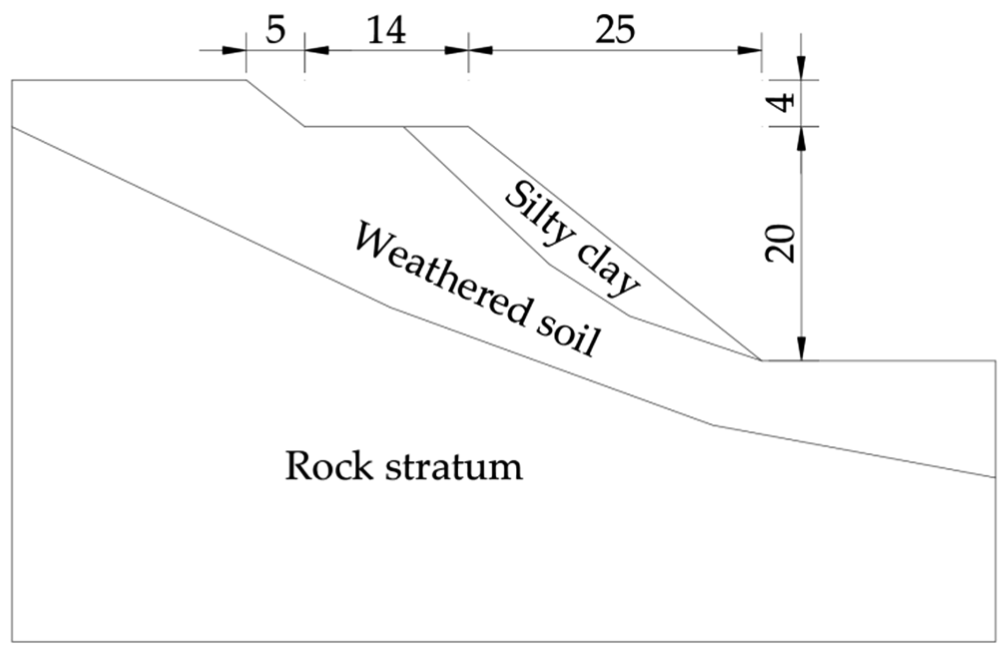
2.1. Engineering Background

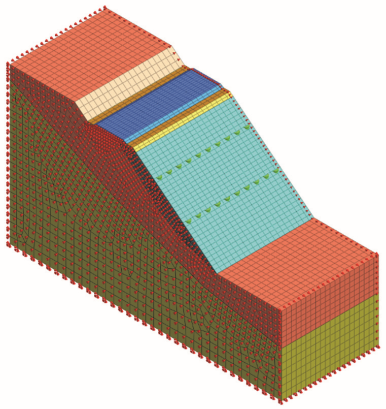
This slope is located in a section of a railway in transition from hills to mountains. The height of the slope is 20 m, and the gradient is 1:1.25. By geological exploration of the engineering site, the distribution of soil layers is shown in Figure 1. The upper part of the slope has a weak soil layer and a sliding surface, which is a potential source of slope instability, while the lower part is a relatively stable rock layer. Anti-slip piles are suitable to reinforce such slopes with obvious sliding surfaces and weak upper soil layers but stable lower parts [18]. Therefore, double-row anti-slip piles were used to reinforce the slope to prevent the sliding of the land and improve the overall stability of the slope.

2.2. Model Overview

The Mohr–Coulomb yield criterion was used for the slope geotechnical body. The material parameters for the slope geotechnical body, ballast bed, bed, and anti-slip piles were taken from field tests and the corresponding design specifications [19], as shown in

Table 1. Material parameters.

Material	Density (kN·m−3)	Elastic Modulus (MPa)	Poisson’s Ratio	Cohesion (kPa)	Internal Friction Angle (°)
Silty clay	19	16	0.30	17	21
Weathered soil	20	70	0.28	27	25
Rock stratum	22	1500	0.28	150	36
Ballast	22	300	0.25	2	40
Subgrade	21	220	0.28	40	30
Anti-slip pile	25	30,000	0.25	-	-

.

The height, width, and thickness of the slope model were 48 m, 84 m, and 30 m respectively. A hybrid grid generator was used to create the grid cells, with the model grid size ranging from approximately 0.75 m to 2 m. The grid at the train load and the slope face was relatively dense, while the grid at the bottom of the model was relatively sparse. The anti-slip piles were simulated with 1D beam cells, while all other materials were simulated with 3D cells. The horizontal and vertical displacements were constrained at the base of the model, and the horizontal displacements were constrained at the sides. The slope model is shown in Figure 2.

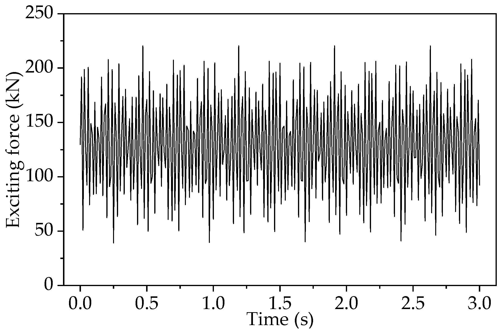
2.3. Train Load Simulation

A train load is affected by the bearing weight, track irregularity, running speed, and subgrade characteristics. The dynamic load of a moving train can be simulated by the excitation force function [20] and the following mathematical expression:

$$F(t)=k_1{k}_2(P_0+P_1\sin {\omega }_{1}t+P_2\sin {\omega }_{2}t+P_3\sin {\omega }_{3}t)$$

(1)

where k₁ is the superposition coefficient between adjacent wheels and rails (k₁ = 1.6); k₂ is the dispersion coefficient between rail sleepers (k₂ = 0.9); P₀ is the static wheel load of the train (P₀ = 90 kN); and P₁, P₂, and P₃ are the typical values of a vibration load under the three types of control conditions, namely track unevenness, train weight with additional dynamic load, and rail surface waveform wear. The corresponding calculation expressions are as follows:

$$p_i=M_0{\alpha }_i{\omega }_i^2(i=1,2,3)$$

(2)

where M₀ is the spring mass of the train (M₀ = 750 kg); α_i is the vector height corresponding to the geometric upset (α₁ = 3.5 mm, α₂ = 0.4 mm, and α₃ = 0.08 mm); ω_i is the circular frequency of the vibration wavelength (ω_i = 2πv/L_i); v is the train travel speed (v = 69.4 m/s); and L_i is the upset curve wavelength (L₁ = 10 m, L₂ = 2 m, and L₃ = 0.5 m). Then, the mathematical expression for the train load and the time curve of the load from 0–3 s (Figure 3) is as follows:

$$F(t)=1.44\times \left[\begin{array}{l}90+5.0\sin (43.6t)\\ +14.3\sin (218.2t)\\ +45.7\sin (872.6t)\end{array}\right]$$

(3)

3. Model Calculation and Analysis

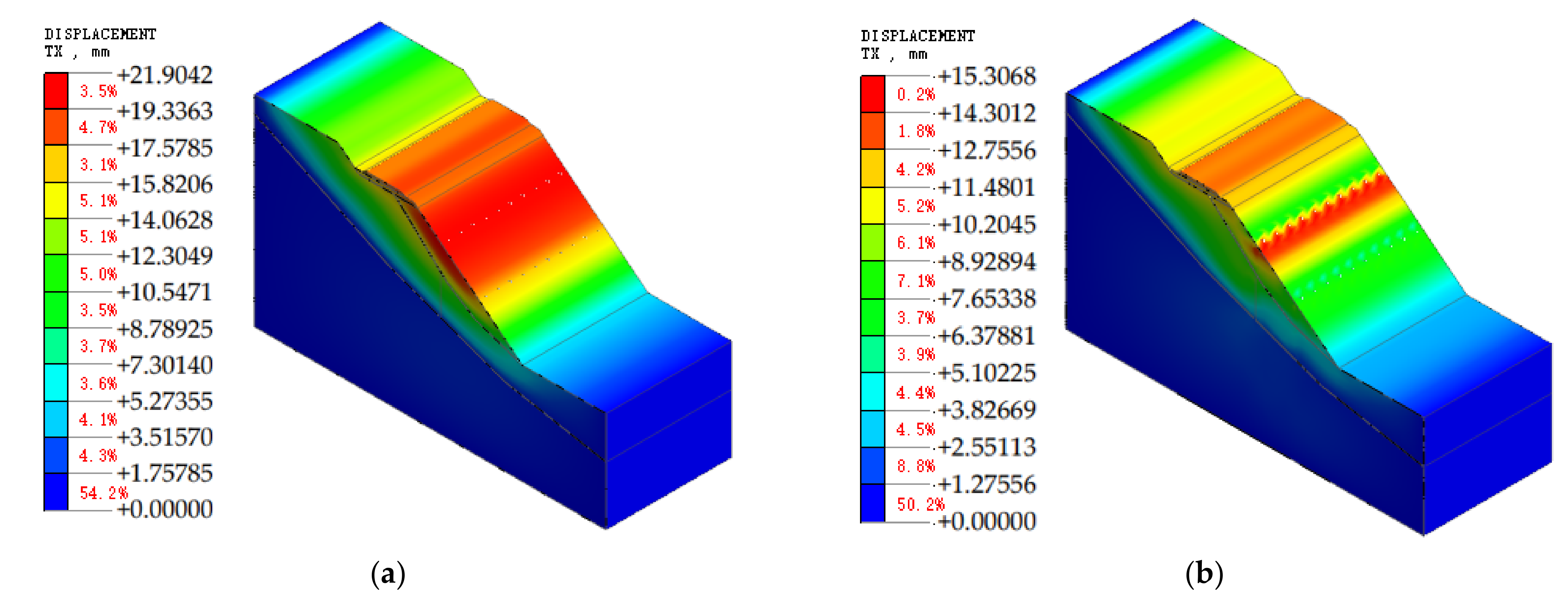
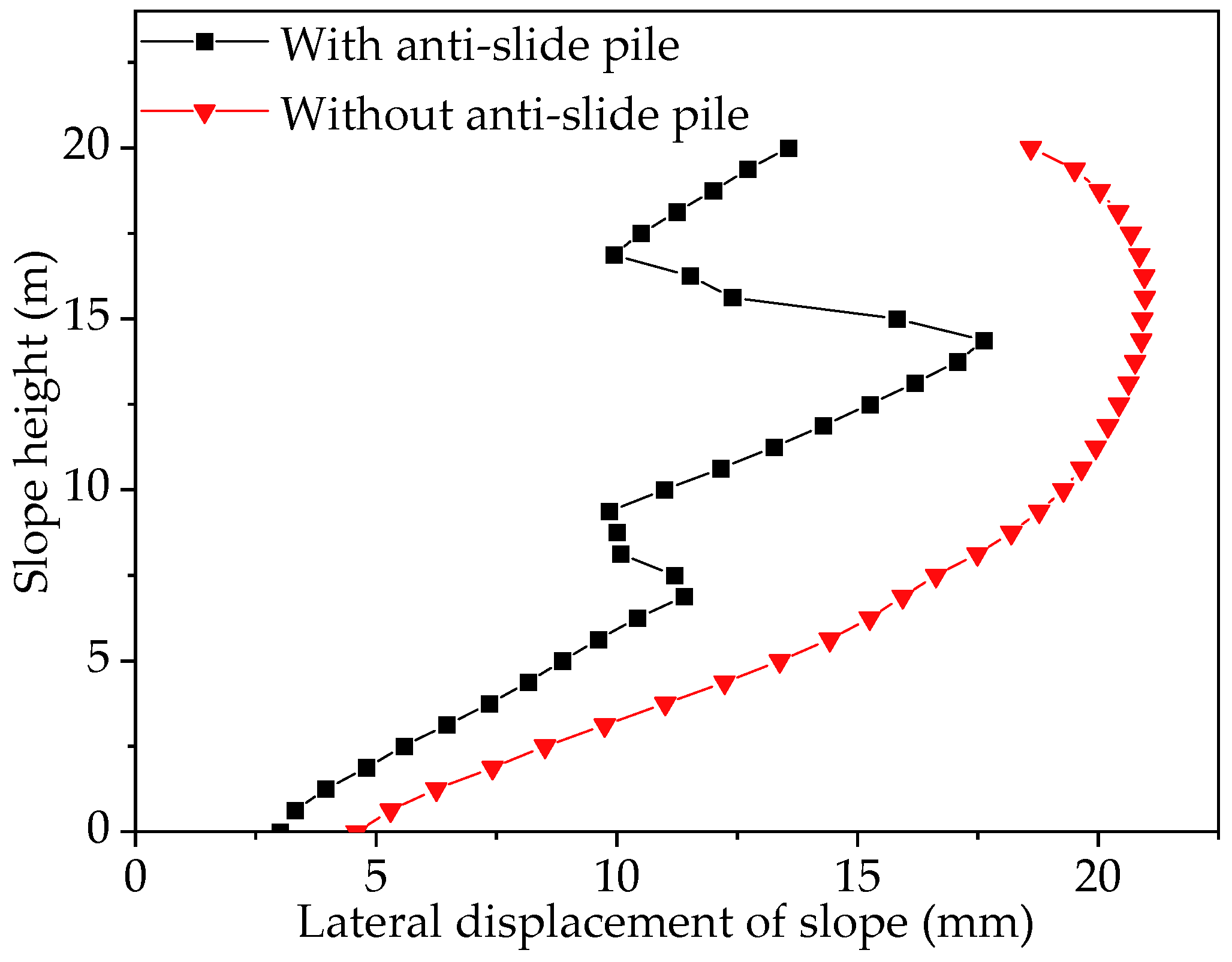
3.1. Effectiveness of Anti-Slip Pile Reinforcement

Using the finite element strength reduction method (SRM) to calculate slope stability coefficients, the basic principle is to divide the cohesive force, c, and the tangent of the angle of internal friction, tanφ, by an increasing coefficient at the same time to obtain the reduced c′ and φ′ for the slope stability analysis, and the corresponding F_st is the slope stability coefficient when the slope happens to be damaged. The calculation formula is as follows:

$$c\prime =c/F_{\mathrm{st}}$$

(4)

$$\phi \prime =\arctan (\tan \phi /F_{\mathrm{st}})$$

(5)

where c′ and φ′ are the cohesion and the angle of internal friction, respectively, when discounting to exactly the point where damage occurs. The criteria for judging slope instability using SRM are mainly the following three aspects: (1) a numerical calculation does not converge; (2) a sudden change in slope displacement occurs; and (3) a slope plastic zone penetrates.

The slope is located on the main railway line. Once a landslide occurs, it will cause immeasurable losses. Referring to the design specification, the required stability factor of safety for this slope is not less than F_st = 1.35 [21]. The stability factor of the slope without reinforcement measures was 1.175, which was not up to the requirement, so corresponding reinforcement measures were required.

Therefore, the slope was supported by two rows of anti-slip piles, the diameter of which were 1.5 m. The length of the upper row of piles was 28 m, the length of the lower row of piles was 22 m, the pile spacing was 3 m, the pile row distance was 9 m, and the horizontal distance of the lower row of piles from the foot of the slope (noted as the pile position) was 10.5 m.

After reinforcement by anti-slip piles, the slope stability factor was increased to 1.680, which was higher than F_st = 1.35, so the anti-slip piles were effective in improving the slope stability. The effect of the anti-slip piles on the stability of the slope was obvious. The lateral displacement nephogram before and after the slope strengthening are shown in Figure 4, and the horizontal displacement of the slope is shown in Figure 5.

As can be seen from the above figure, before the anti-slip pile reinforcement, the lateral displacement of the slope increased and then decreases with the rise in the slope height; the corresponding lateral displacement of the slope at the slope height of 12–18 m was maintained at a higher level of 20 mm or more, and at the slope height of 13 m, the lateral displacement of the slope reached a maximum of 21.1 mm.

After the slope was reinforced by anti-slip piles, the lateral displacement also decreased accordingly. When the slope height was about 9 m and 17 m, the lateral displacement of the slope reached its minimum value, which rapidly decreases to about 9.8 mm. These two places were located near the anti-slip pile, so the slope was more constrained by the anti-slip pile than at other locations. In the slope away from the anti-slip pile, with the gradual elimination of the anti-slip pile supporting effect, the lateral displacement of the slope also began to increase, but it was still lower than the corresponding slope without support. The maximum of slope lateral displacement was 15.3 mm, which was located at the height of 14.5 m. Compared with before reinforcement, the maximum lateral displacement of the slope was reduced by 27.5%. Overall, the anti-slip pile had a certain constraint on the lateral displacement of the slope.

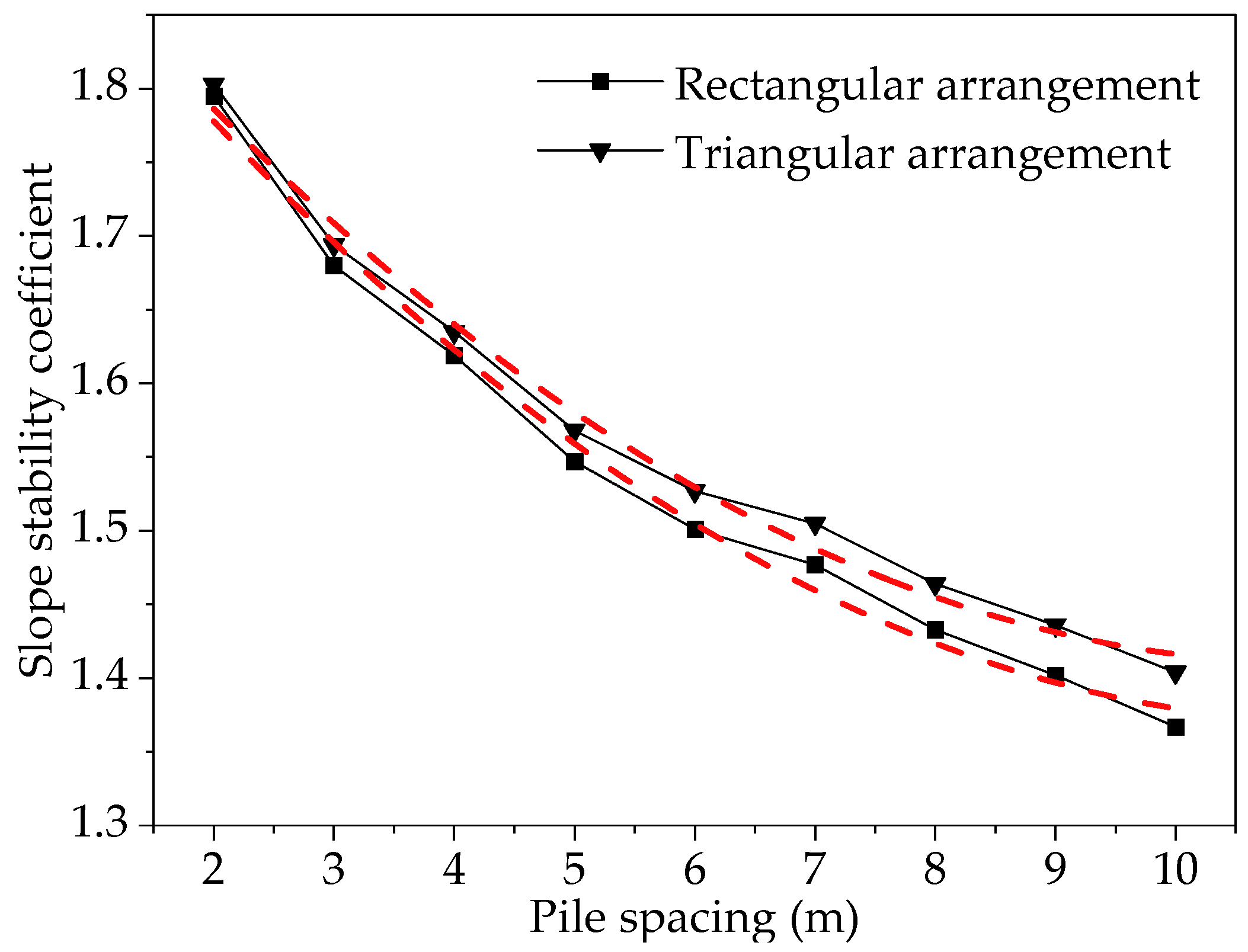
3.2. Analysis of the Effect of Anti-Slip Pile Spacing

In order to study the influence of anti-slip pile spacing and pile arrangement on the slope reinforcement effect, the anti-slip pile spacing was divided into nine working conditions from 2 m to 10 m, and the upper and lower rows of anti-slip piles were arranged in rectangular and triangular rows. The anti-slip pile layout is shown in Figure 6.

The stability of the slope under different pile spacings is shown in Figure 7. With an increase in the anti-slip pile spacing, the reinforcement effect of the anti-slip piles on the slope gradually decreased and the stability of the slope also decreased, but the overall decline tended to slow, and there was an inflection point near 7 m, after which the decline slowly expanded again.

Taking the rectangular arrangement as an example, the slope stability coefficient was 1.795 when the anti-slip pile spacing was 2 m. When the anti-slip pile spacing was increased to 10 m, the corresponding slope stability coefficient was 1.367, which was slightly higher than F_st = 1.35, and actual pile spacing rarely reaches 10 m. The reinforcement effect of anti-slip piles with a triangular arrangement was slightly better than that of a rectangular arrangement. The larger the pile spacing, the more significant the difference between the two types of arrangements.

The reason is that, when the anti-slip piles are arranged in a rectangular configuration, the slope section between the two rows of anti-slip piles is not directly supported, and the possibility of damage in this section is higher than in the section where the anti-slip piles are arranged; whereas when the anti-slip piles are arranged in a triangular configuration, the restraining effect of the anti-slip piles on the landslide body is better spread to other sections of the slope, and the overall stability of the slope is improved.

In addition, the function expression of the slope stability coefficient, F_S, with respect to pile spacing, a, can be obtained by fitting the curve in Figure 7:

Rectangular arrangement:

$$F_S=0.7662e^{-0.2017a}+1.2726$$

(6)

Triangular arrangement:

$$F_S=0.7141e^{-0.2117a}+1.3254$$

(7)

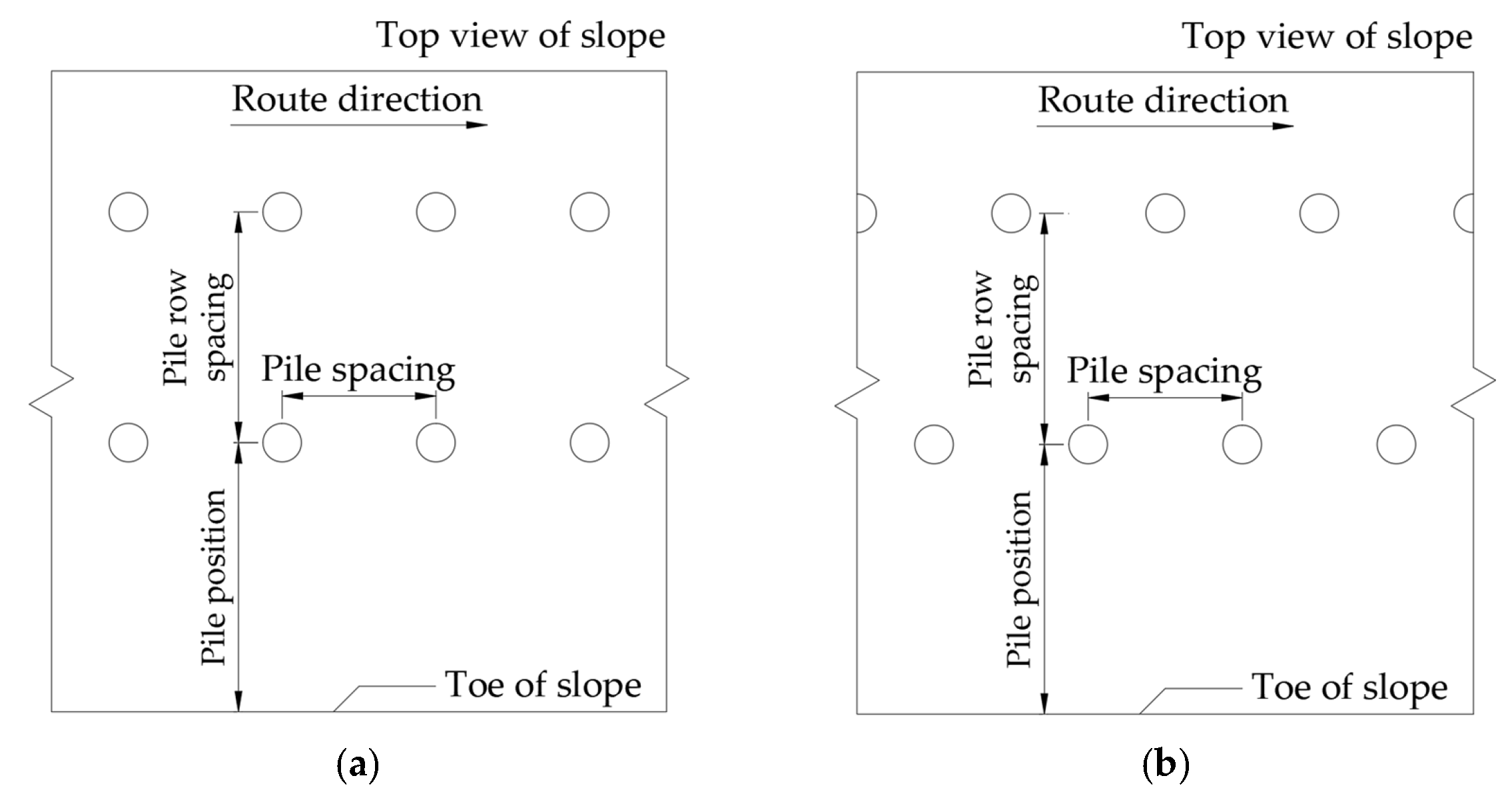
3.3. Analysis of the Impact of Anti-Slip Pile Placement Locations

The layout position of the anti-slip piles on the slope mainly includes two factors: the horizontal distance between the upper and lower rows of piles (pile row spacing) and the horizontal distance of the lower row of piles from the foot of the slope (pile position). By studying the variation in these factors, the optimal placement of anti-slip piles can be determined to improve the efficiency of anti-slip pile support and save construction costs as much as possible.

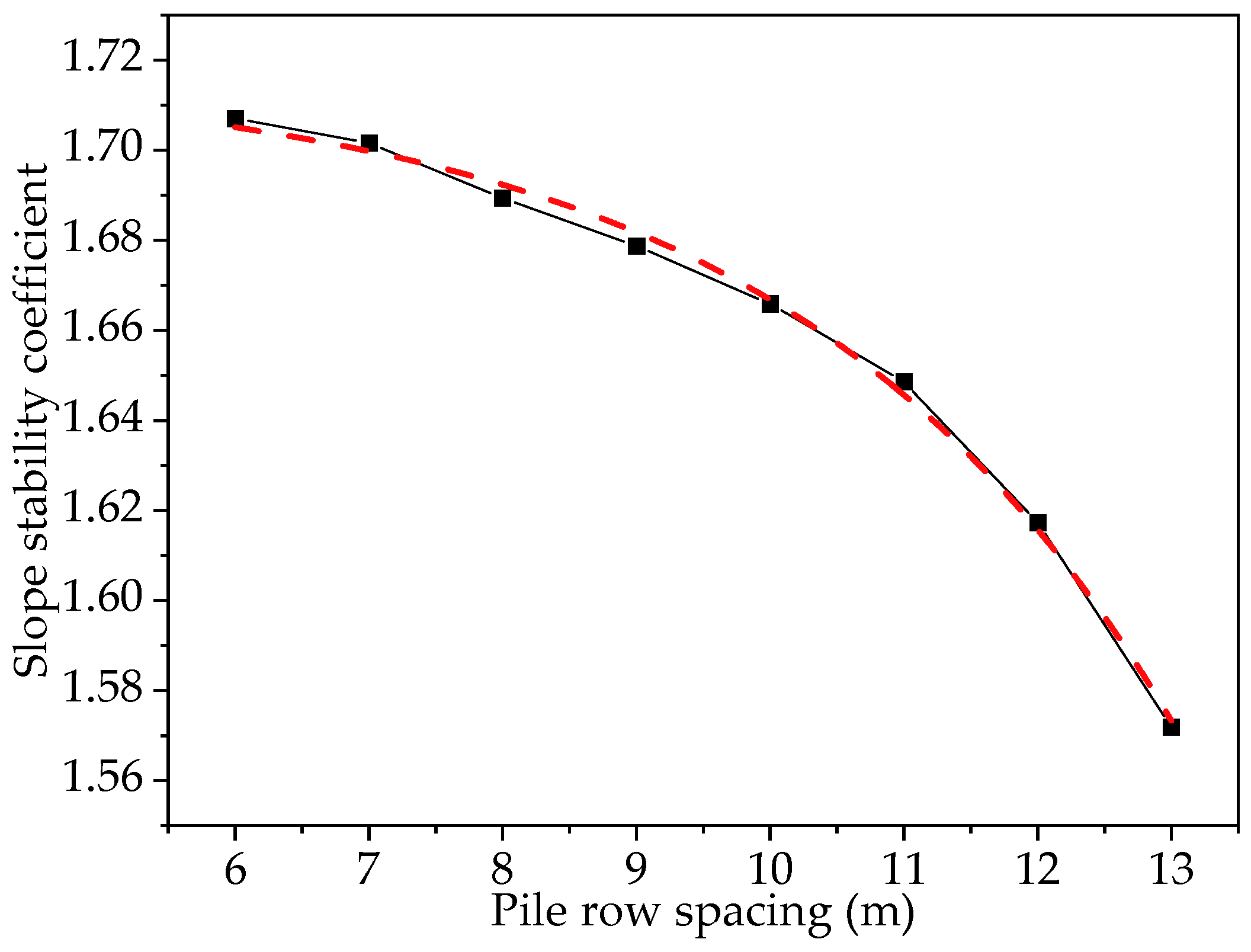
3.3.1. Pile Row Spacing

The pile position was 10.5 m, and the pile spacing was 3 m. The stability of the slope was analyzed for pile rows ranging from 6 m to 13 m. The effect of pile spacing on slope stability was obtained through finite element analysis and is shown in Figure 8.

The slope stability coefficient tended to decrease gradually as the pile spacing increased. When the pile spacing was 6–7 m, the stability coefficient of the slope remained high, and the corresponding stability coefficient was maintained at about 1.7. After 10 m, the stability of the slope began to decline at an accelerated rate, with a corresponding stability coefficient of 1.579 at 13 m. It can be inferred that the central part of the slope was more unstable than the rest of the slope and was at the greatest risk of instability, which should be considered in the actual construction.

The function expression of the slope stability coefficient, F_S, with respect to pile row spacing, b, can be obtained by fitting the curve in Figure 8:

$$F_S=-0.0016e^{0.3474b}+1.7179$$

(8)

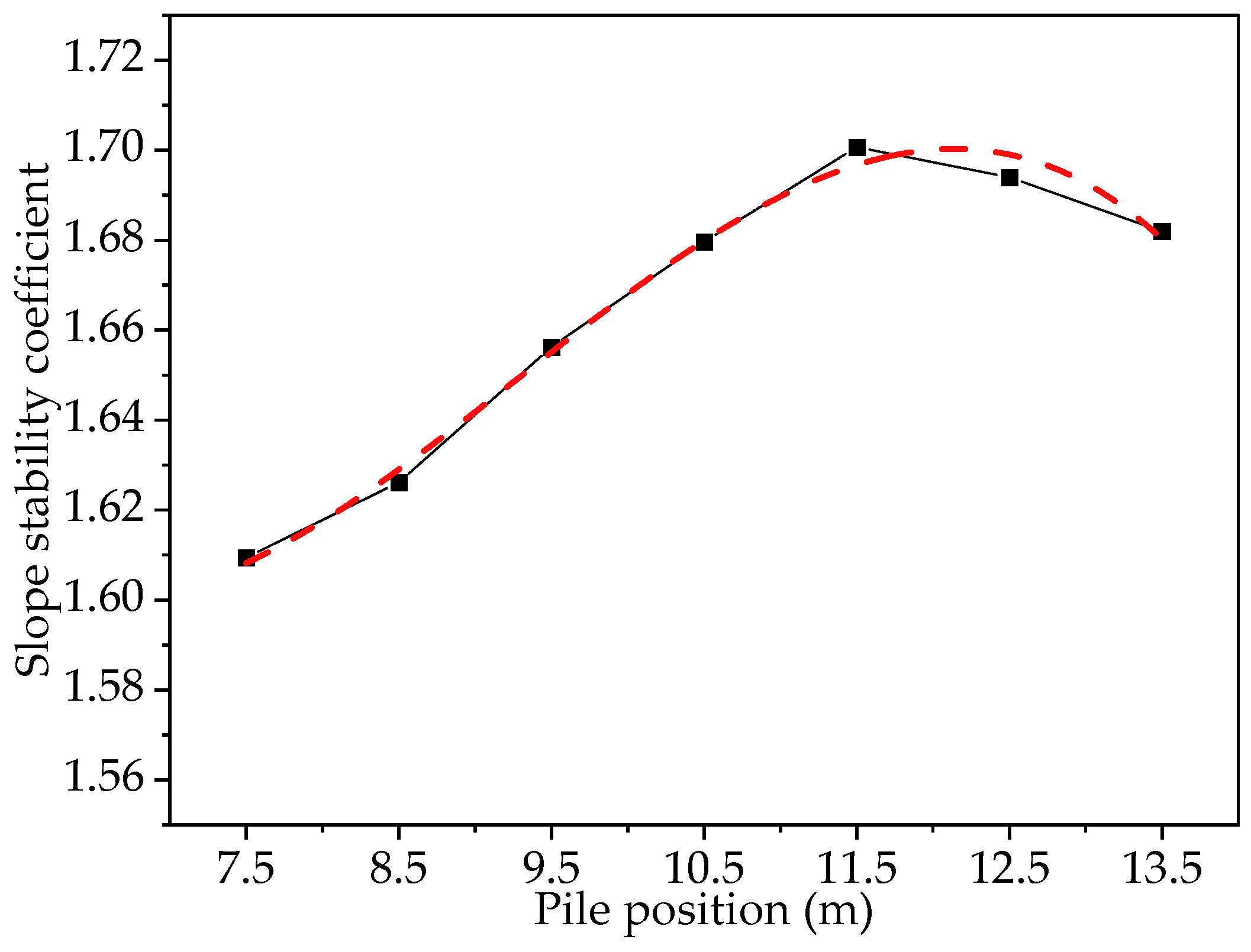
3.3.2. Pile Position

Taking the pile spacing as 3 m and the pile row spacing as 9 m, the change in slope stability for the pile position from 7.5 m to 13.5 m was studied, as shown in Figure 9.

The results show that the slope stability coefficient rose first and then fell as the pile position increased, with the slope being most stable at 11.5 m and the slope stability coefficient reaching a peak of 1.701. Therefore, it was more effective to place the anti-slip piles at a slightly higher position in the middle of the slope to strengthen the slope.

The reason why the slope stability coefficient turned at 11.5 m is because the slope stability was affected by the pile position. If the position of the anti-slip pile on the slope was too low or high, it did not improve the slope stability much; only when the anti-slide pile was laid in a suitable position could the slope stability coefficient reach the maximum value.

The function expression of the slope stability coefficient, F_S, with respect to the pile row spacing, c, can be obtained by fitting the curve in Figure 9:

$$F_S=-0.0011c^3+0.0307c^2-0.2593c+2.2883$$

(9)

The different locations of the anti-slip piles had an impact on the stability of the slope, mainly because the reinforcement of two rows of piles divided the original potential sliding surface of the whole slope into three areas; the change in the location of the anti-slip piles made the areas of these three sliding bodies change, and the stability of the slope was mainly determined by the weakest area. If the anti-slip piles were not reasonably located on the slope, all of them caused an excessive volume in a certain area, resulting in a reduction in the safety of the slope.

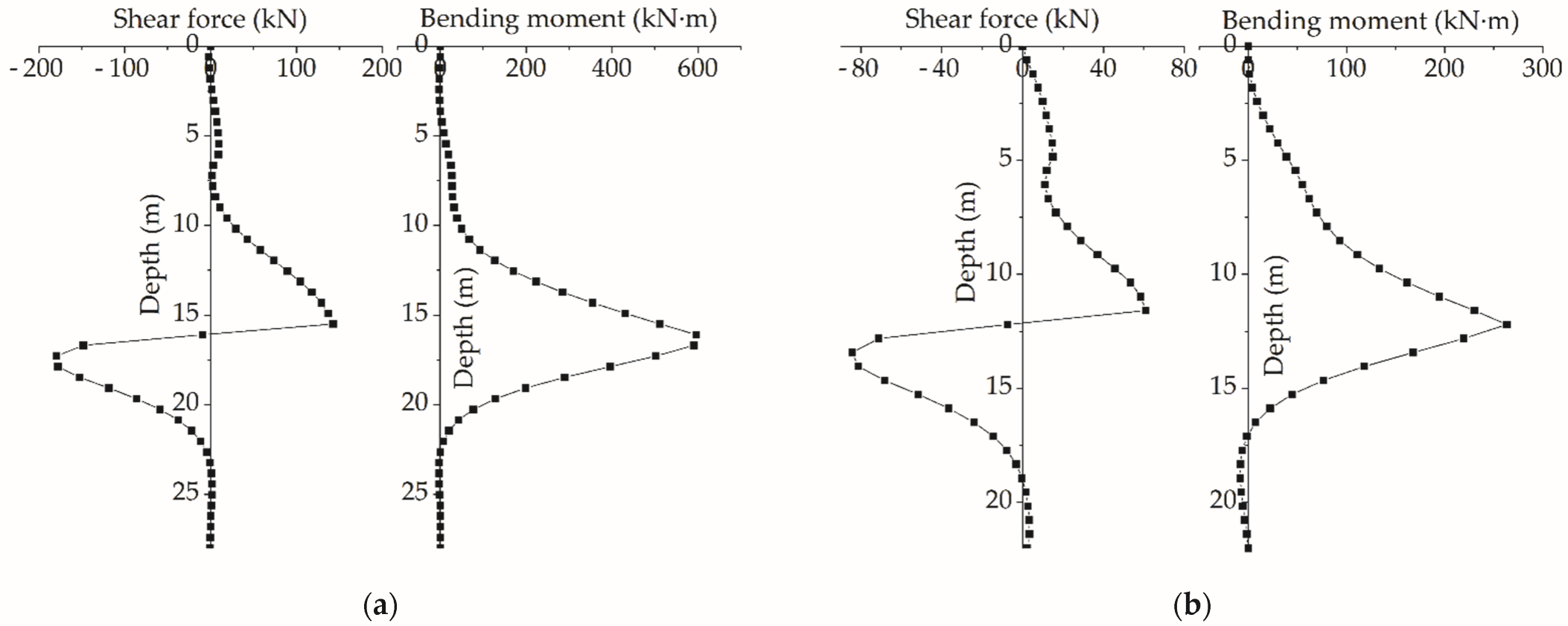
3.4. Internal Pile Force Analysis

Based on the same strength, size, and layout of anti-slip piles, with an anti-slip pile spacing of 3 m, row spacing of 9 m, and pile position of 10.5 m, as an example, the distribution of shear forces and bending moments in the two rows of piles are shown in Figure 10.

According to the analysis results, the unfavorable sections of two rows of piles were in the middle and lower parts. The maximum bending moment points of the upper and lower rows of piles were located at 16.1 m and 12.2 m of pile depth, respectively. There was a reverse bending point in the lower part of the piles, and the reverse bending moment was much smaller than the positive bending moment.

The maximum internal forces of the two rows of piles are compared in

Table 2. Internal force comparison of anti-slip piles.

	Upper Row of Piles	Lower Row of Piles	Ratio
Maximum shear force (kN)	179.3	84.3	2.13
Maximum bending moment (kN·m)	595.9	267.7	2.23
Maximum stress (kPa)	1326.9	610.3	2.17

. The shear forces, bending moments, and maximum stresses within the upper row of piles were greater than those in the lower row, and the internal forces in the upper row were approximately 2.2 times greater than those in the lower row. The upper anti-slip piles were subjected to higher train loads, and the upper piles shared a certain amount of earth pressure, resulting in the lower piles generally being subjected to less force than the upper piles. In practice, the upper row of anti-slip piles can be increased in diameter and spacing to improve their resistance to damage, or pre-stressed anchors can be added to improve the force of anti-slip piles.

4. Analysis of the Pile–Soil Action of Anti-Slip Piles

The design and layout of anti-slip piles should also consider the influence of pile–soil interactions. However, the distribution graph of landslide thrust and earth pressure on the pile side is difficult to calculate. It is affected by multiple factors such as the physical and mechanical properties of the soil, soil structure, and additional forces. Therefore, we used finite element software and theoretical calculation methods to focus on the upper row of piles for earth pressure and landslide thrust analyses and finally verified them through engineering examples.

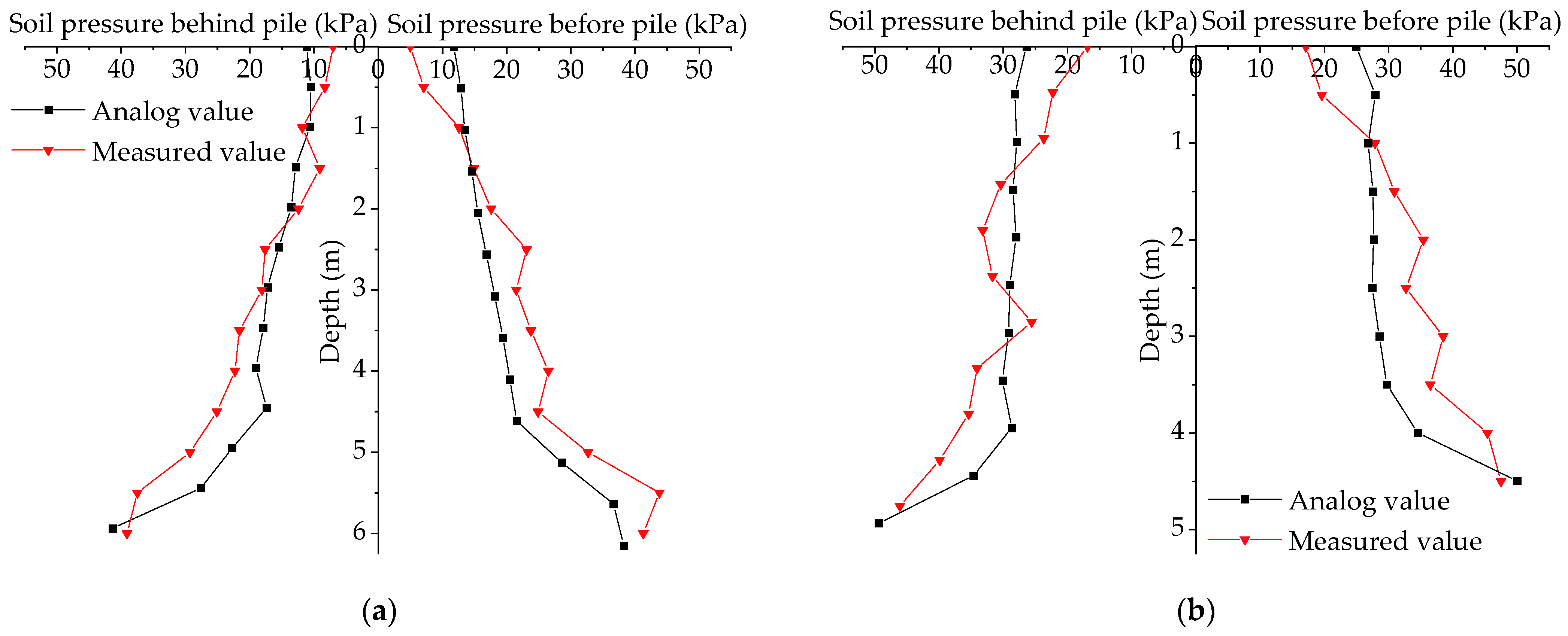
4.1. Analysis of Earth Pressure on Pile Side

Earth pressure cells were used to monitor the earth pressure of the landslide section, and one monitoring point was set every 0.5 m in the vertical direction. The upper row of pile measurement points was arranged as 13 behind and 13 in front of the pile; the lower row of pile measurement points was arranged as 11 behind and 10 in front of the pile. The measured soil pressure values were plotted as distribution curves and compared with the finite element simulation results, as shown in Figure 11.

The curve in Figure 11 shows that the earth pressure on the pile side generally increased with an increase in pile depth, with an approximately trapezoidal distribution, and there was an obvious mutation near the sliding surface. From the field-measured data of earth pressure, the distribution law was basically consistent with the finite element simulation results. The measured values of earth pressure at a pile depth of 0–1 m were smaller than the finite element simulation values, but from a pile depth of 1 m below until the soil layer boundary, except for a few points, the measured values were larger than the finite element simulation values.

This phenomenon was caused, firstly, by the sliding surface, which was at the soil boundary, where the different soil material parameters, the possible interaction between the two rows of piles, and the superimposed effect of the train load produced stress redistribution and relative displacement. Furthermore, the uppermost potential landslide area (mainly the silty clay layer) was the weakest part of the soil, and the self-weight of the soil and the transfer of the train load increased the sliding tendency of the land, which was also an important reason for the steep increase in earth pressure at the sliding surface.

The Coulomb earth pressure theory was used to calculate the magnitude of the earth pressure above the sliding surface of the two rows of piles. According to the force characteristics, the active earth pressure was behind the pile and the passive earth pressure was front of the pile. The theoretical results are compared with the finite element analysis and engineering measurements in

Table 3. Calculation results of pile-side earth pressure (unit: kN).

		Theoretical Value	Analog Value	Theoretical Value/Analog Value
Upper row of piles	Earth pressure behind pile	98.1	102.1	0.96
	Earth pressure before pile	719.3	124.8	5.76
Lower row of piles	Earth pressure behind pile	140.5	152.6	0.92
	Earth pressure before pile	926.1	133.7	6.93

.

From the data in Table 3:

• The active earth pressure values behind the pile calculated by the Coulomb earth pressure theory were about 4–8% lower than the finite element analog results. This was mainly because the Coulomb earth pressure theory did not consider the deformation of the pile and the soil in the actual force process. The actual sliding surface was not flat, which caused deviations between the theoretical results and the finite element simulation.
• The passive earth pressure values before the pile calculated by the Coulomb earth pressure theory were 5–7 times greater than the finite element analog values. Therefore, it is not suitable to use the Coulomb passive earth pressure theory, which is also consistent with conventional experience.

4.2. Landslide Thrust Analysis

In railway design specification, it is usually assumed that the body slides uniformly along the sliding surface, and the explicit solution method of the transfer coefficient method is usually used in railway engineering to determine the landslide thrust [22]. The calculation formula is as follows:

$$T_i=K{W}_i\sin {\alpha }_i+\psi T_{i-1}-W_i\cos {\alpha }_i\tan {\phi }_i-c_i{L}_i$$

(10)

$$\psi =\cos ({\alpha }_{i-1}-{\alpha }_i)-\sin ({\alpha }_{i-1}-{\alpha }_i)\tan {\phi }_i$$

(11)

where T_i is the landslide thrust at the end of the ith soil bar; K is the slope safety factor; W_i is the gravity of the ith soil bar; α_i is the inclination of the sliding surface corresponding to the ith soil bar; φ_i is the friction angle at the bottom of the ith soil bar; c_i is the cohesion at the bottom of the ith soil bar; L_i is the length of the sliding surface of the ith bar; and ψ is the (i − 1)th soil bar transfer coefficient.

In addition, the landslide thrust can also be determined using the implicit solution of the transfer coefficient method. Different from the explicit solution, the implicit solution divides the anti-sliding force by the safety factor and is calculated as follows:

$$T_i=W_i\sin {\alpha }_i+\psi T_{i-1}-(W_i\cos {\alpha }_i\tan {\phi }_i-c_i{L}_i)/K$$

(12)

The letters in the form represent the same meanings as above.

It is worth noting that differences in the formulas (explicit or implicit methods) or safety factor K will cause different theoretical results, as detailed in

Table 4. Results of landslide thrust (unit: kN).

		K	Theoretical Value	Analog Value	Theoretical Value/Analog Value
Upper row of piles	Explicit method	1.00	96.3	89.2	1.08
		1.35	265.6		2.98
	Implicit method	1.00	96.3		1.08
		1.35	197.6		2.21
Lower row of piles	Explicit method	1.00	146.4	123.1	1.19
		1.35	389.9		3.16
	Implicit method	1.00	146.4		1.19
		1.35	296.7		2.41

.

The results in Table 4 reflect:

• When the safety factor K = 1.00, the results calculated using the transfer coefficient explicit method and implicit method were the same. The theoretical values were close to (8–19% higher than) the finite element simulation values.
• When the safety factor K = 1.35, the theoretical values were much larger than the finite element values, and the results calculated by the explicit method were larger than those calculated by the implicit method. In addition, the results of the explicit method were approximately three times higher than the finite element values, while the results of the implicit method were approximately 2.3 times higher than the finite element values.

The reason why the railway specification adopted the explicit method to calculate the landslide thrust and introduced a safety factor is that railway has suffered greater loads and needs to consider more unfavorable conditions in the design to ensure the safety and stability of the slope, which ultimately makes the theoretically calculated landslide thrust value larger than the finite element simulation value. In addition, the transfer coefficient method assumes that the slide is a rigid body and does not consider the relative deformation of the soil within the slide, which was also one of the reasons for the large calculation results.

4.3. Engineering Example Validation

Through a field test, the measured values of landslide thrust, and earth pressure were compared with the finite element simulation values, as shown in

Table 5. Comparison of measured values of pile–soil interaction.

		Measured Value (kN)	Measured Value/Analog Value
Upper row of piles	Earth pressure behind pile	119.5	1.17
	Earth pressure before pile	142.2	1.14
	Landslide thrust	98.7	1.11
Lower row of piles	Earth pressure behind pile	160.8	1.05
	Earth pressure before pile	149.6	1.12
	Landslide thrust	138.9	1.13

.

From the measured results, it was found that the measured values of the pile-side earth pressure and the landslide thrust for the upper row of piles were 11–17% higher than the finite element simulation results; those for the lower row of piles were 5–13% higher than the finite element simulation values. The relative deviations were within the acceptable limits, and the simulated results can be relatively reliable.

The measured results were slightly larger than the finite element results. This was related to the errors caused by finite element meshing and modeling calculations, and the finite element simulation does not consider more unfavorable factors. Therefore, it is necessary to make anti-slip piles more safety-biased in design and reduce the possibility of landslide occurrence by introducing safety factors into the theoretical calculation.

5. Unfavorable Condition Analysis

The railway slope was in a hilly mountainous area, where natural disasters are frequent. To research whether the anti-slip piles had a sufficient reinforcement effect, we simulated two unfavorable conditions, namely rainfall and an earthquake, and compared and analyzed the stability, lateral displacement, and plastic zone range of the slope before and after reinforcement under these two conditions with 3 m anti-slip pile spacing, 9 m row spacing, and a 10.5 m pile position.

Due to limited space, this section only briefly analyses the rainfall and seismic conditions of the slope.

5.1. Rainfall Conditions

Rainfall conditions consider the reduction in material parameters above the rock–soil interface and the unsaturated characteristics of the soil. Combined with local meteorological data, the rainfall intensity was taken as 10 mm/h for 2 days.

Based on the finite element model in Figure 2, the slope surface, slope top, and slope foot of the model were taken as the rainfall infiltration surface; the bottom of the model was set as an impermeable boundary. Through the finite element analysis, the distribution of the slope plastic zone under the rainfall condition is shown in Figure 12.

The results of the numerical analysis show that the stability coefficient of the slope after the rainfall condition was 1.545, and the pore water pressure inside the slope increased with the infiltration of rainfall. After two days of rainfall simulation, the maximum lateral displacement of the slope supported by anti-slip piles was 28.6 mm, which was 34.3% lower than the 43.5 mm of the maximum lateral displacement before the anti-slip pile reinforcement. At the same time, the extent of the plastic zone was also significantly reduced and was mainly concentrated at the parting of the soil layers, with a maximum strain of 2.91 × 10⁻³, a reduction of 39.6% compared to the maximum plastic strain of 4.82 × 10⁻³ before the anti-slip pile reinforcement. The maximum strain was in the upper part of the slope, adjacent to the load, which should be noted in practical engineering, and corresponding measures should be taken to dispose of it if necessary.

In addition, the shear and bending moments of the piles under rainfall conditions are shown in Figure 13. The maximum bending moment of the anti-slip piles was 682.4 kN·m, and the maximum shear force was 223.4 kN, both of which were in the lower row of piles. This was contrary to the conclusion in Section 3.4 that the upper row of anti-slip piles is subjected to greater forces than the lower row of piles. The main reason is that rainfall increased the weight of the soil, and the soil sliding force increased and acted on the anti-slip pile; the lower row of anti-slip piles was subjected to a large amount of overlying earth pressure, and this effect was more significant due to the downward seepage of water in the soil, so the sliding force of the soil was also greater than that of the upper row of anti-slip piles. According to the results of the finite element simulation, the whole slope was safe under the rainfall condition of this intensity.

5.2. Seismic Conditions

The seismic protection intensity in this area is taken to be 8 degrees [23]. Based on the finite element model in Figure 2, a free field was applied to both sides of the slope model, and a fixed constraint was applied at the base of the model. Then, the EI Centro horizontal seismic wave was used to simulate the seismic accelerations and to determine the time-dependent load functions as well as the eigenvalues.

By simulating the slope model under seismic conditions, the maximum lateral displacement of the slope was 24.2 mm after reinforcement by anti-slip piles, which was 57.0% less than the 56.3 mm of displacement of the slope without reinforcement, and that of the upper part of the slope was generally larger.

In addition, the extent of the plastic zone was also significantly reduced, as shown in Figure 14. The maximum plastic strain was located at the junction of the weathered soil and rock strata, corresponding to 1.58 × 10⁻³, which was 46.3% lower than that of 2.94 × 10⁻³ without reinforcement. The plastic zone of the slope after the anti-slip pile reinforcement was mainly located at the intersection of the rock and soil and behind the anti-slip piles. The stability coefficient of the slope under seismic load was 1.304, which was greater than the corresponding safety factor, F_st = 1.15 [21]. The slope remained safe after an earthquake of this intensity.

The maximum horizontal displacements of the anti-slip piles that occurred under earthquake action are shown in Figure 15. The maximum displacements of the upper and lower rows of piles occurred at the tops of the piles, which were 18.5 mm and 13.1 mm, respectively, and the horizontal displacement of the upper row of piles was 41.2% larger than that of the lower row of piles. As the pile depth increased, the horizontal displacement of the anti-slip piles gradually decreased; the bottom displacement of both rows of piles was about 2 mm.

6. Conclusions

Based on the engineering background of a railway slope, Midas GTS NX software was used to establish a finite element model in this paper. First, the influences of anti-slip pile spacing, row spacing, and pile position on slope stability were analyzed. Second, the stress of anti-slip piles and the distribution law of earth pressure on the pile side were studied. Then, the Coulomb earth pressure theory and the transfer coefficient method were compared and verified by measured values. Finally, the slope in two unfavorable conditions of rainfall and an earthquake were studied. The conclusions are as follows:

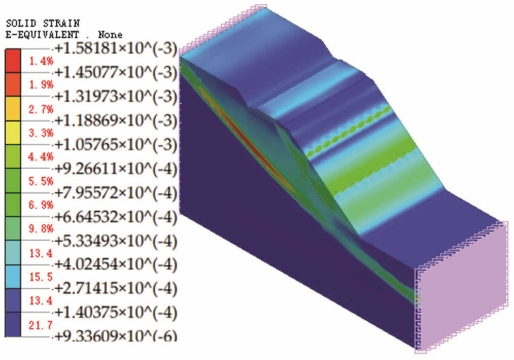
• After the support of anti-slip piles, the slope stability coefficient increased significantly from 1.175 to 1.680; the maximum horizontal displacement of the slope was also reduced by 27.5%.
• The slope stability decreased gradually with an increase in anti-slip pile spacing. The supporting effect of anti-slip piles with a triangle layout was slightly better than with rectangle layout, which was more obvious when the spacing of the anti-slip piles was large.
• With an increase in the pile row spacing, the slope stability gradually decreased, and the rate of decline accelerated. When the pile position gradually increased, the slope stability first increased and then decreased, and the slope corresponding to the pile position of 11.5 m was the most stable.
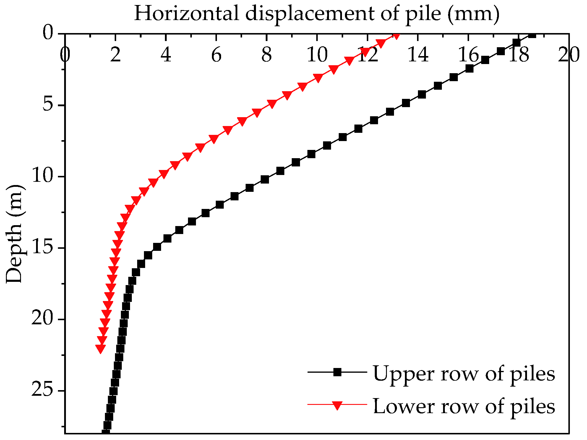
• The most unfavorable section of two rows of anti-slip piles was in the lower part of the pile body, where two rows of piles had a reverse bending point, which was much smaller than the positive bending moment. The internal force of the upper pile was about 2.2 times that of the lower pile.
• The earth pressure on the sliding surface increased with an increase in pile depth which was a roughly trapezoidal distribution, and there was a significant mutation near the soil interface. The active earth pressure values behind the piles calculated by Coulomb’s theory were 4–8% lower than the finite element values. The passive earth pressure values before the piles were much larger than those of the finite element analysis.
• The transfer coefficient method was used to calculate landslide thrust. When K = 1.00, the calculation results of the explicit method and the implicit method were the same, which were 8–19% higher than the finite element results. When K = 1.35, the theoretical values of the explicit method were about three times higher than the simulation values, and those of the implicit method were about 2.3 times higher than the simulation values.
• The measured values verified that the simulated values had a certain degree of reliability, and the relative deviation between the two was 5–17%.
• The reinforced slope remained stable under both rainfall and earthquake conditions; the maximum lateral displacement and plastic strain of the slope under rainfall conditions were reduced by 34.3% and 39.6%, respectively, compared with those under unsupported conditions, while the corresponding reductions in seismic conditions were 57.0% and 46.3%.

References

1. Zhang, Z. Numerical Analysis of Load Influence Parameters on Subgrade Slope Stability. Transp. Sci. Technol. 2018, 4, 45–47. [Google Scholar]
2. Wei, M.; Feng, X.; Gao, P.; Liu, J. Stability Analysis of Railway High Embankment Under Heavy Load. Fly Ash Compr. Util. 2021, 35, 118–122. [Google Scholar]
3. Cheng, A.; Yan, Y.; Li, J.; Zhang, Y.; Dai, S.; Dong, F. Stability Analysis and Reinforcement Measures of High and Steep Slopes of Cheng-Lan Railway. Eng. J. Wuhan Univ. 2021, 54, 515–523+578. [Google Scholar]
4. Jia, X.; Xu, J.; Wu, L.; Han, Y. Permanent Displacement Analysis of Road Slope Under Earthquake Load. J. Chang. Univ. (Nat. Sci. Ed.) 2014, 34, 13–18. [Google Scholar]
5. Fang, J.; Deng, H.; Li, J.; Qu, D. Effector of Pile-soil Stiffness Ratio and Pile Distribution on Pile Internal Force Distribution. J. Disaster Prev. Mitig. Eng. 2019, 39, 487–493. [Google Scholar]
6. Rao, P.; Zhao, L.; Liu, Y.; Li, L. Extended 3D Stability Analysis of a Slope Reinforced with Piles Using Upper-bound Limit Analysis Method. Adv. Eng. Sci. 2018, 50, 184–192. [Google Scholar]
7. Wang, X.; Xia, L. Anti-slip Pile Strength and Pile Position Factor-based Study on Safety and Stability of Slope. Water Resour. Hydropower Eng. 2020, 51, 152–158. [Google Scholar]
8. Xu, H.; Xia, Q.; Wang, X. Sensitivity Analysis of Influencing Factors of Slope Safety Coefficient. Railw. Eng. 2021, 61, 98–101. [Google Scholar]
9. Wu, K.; Ding, C. Sensitivity Analysis on Slope Stability Factor Based on Orthogonal Test. J. East China Jiaotong Univ. 2016, 33, 114–120. [Google Scholar]
10. Olgun, M.; Acar, M.H. Investigation of Factors Affecting The Stability of Slopes Subjected to Earthquake Forces. Selçuk Üniversitesi Mühendislik Bilim Teknol. Derg. 2009, 02, 9–20. [Google Scholar]
11. Jing, J.; Hou, J.; Sun, W.; Chen, G.; Ma, Y.; Ji, G. Study on Influencing Factors of Unsaturated Loess Slope Stability under Dry-Wet Cycle Conditions. J. Hydrol. 2022, 612, 128187. [Google Scholar] [CrossRef]
12. Karthik, A.V.R.; Manideep, R.; Chavda, J.T. Sensitivity analysis of slope stability using finite element method. Innov. Infrastruct. Solut. 2022, 7, 184. [Google Scholar] [CrossRef]
13. Dolojan, N.L.; Moriguchi, S.; Hashimoto, M.; Terada, K. Mapping method of rainfall-induced landslide hazards by infiltration and slope stability analysis. Landslides 2021, 18, 2039–2057. [Google Scholar] [CrossRef]
14. Nakajima, S.; Abe, K.; Shinoda, M.; Nakamura, S.; Nakamura, H. Experimental study on impact force due to collision of rockfall and sliding soil mass caused by seismic slope failure. Landslides 2020, 18, 195–216. [Google Scholar] [CrossRef]
15. Zhuang, Y.; Hu, S.; Song, X.; Zhang, H.; Chen, W. Membrane Effect of Geogrid Reinforcement for Low Highway Piled Embankment under Moving Vehicle Loads. Symmetry 2022, 14, 2162. [Google Scholar] [CrossRef]
16. Zhang, B.; Fan, Q.; Luo, J.; Mei, G. A New Analysis Method Based on the Coupling Effect of Saturation and Expansion for the Shallow Stability of Expansive Soil Slopes. Symmetry 2022, 14, 898. [Google Scholar] [CrossRef]
17. Guo, M.-Z.; Gu, K.-S.; Wang, C. Dynamic Response and Failure Process of a Counter-Bedding Rock Slope under Strong Earthquake Conditions. Symmetry 2022, 14, 103. [Google Scholar] [CrossRef]
18. Wei, Y.; Yang, J. Overview of slope geological disaster prevention technology. Subgrade Eng. 2000, 6, 4–7. [Google Scholar]
19. GB 50010-2010; Code for Design of Concrete Structures. China Architecture and Building Press: Beijing, China, 2010.
20. Liang, B.; Luo, H.; Sun, C. Simulated Study on Vibration Load of High-Speed Railway. J. China Railw. Soc. 2006, 28, 89–94. [Google Scholar]
21. GB 50330-2013; Technical Code for Building Slope Engineering. China Construction Industry Publishing: Beijing, China, 2013.
22. TB 10025-2019; Code for Design of Retaining Structure of Railway Earthworks. China Railway Publishing House: Beijing, China, 2019.
23. GB 50111-2006; Code for Seismic Design of Railway Engineering. China Planning Press: Beijing, China, 2006.
Figure 1. Soil layer of the slope (in m).
Symmetry 14 02291 g001
Figure 2. Finite element model of the slope.
Symmetry 14 02291 g002
Figure 3. Train load time-course curve.
Symmetry 14 02291 g003
Figure 4. (a) Lateral displacement nephogram of slope mode before reinforcement. (b) Lateral displacement nephogram of slope mode after reinforcement.
Symmetry 14 02291 g004
Figure 5. Comparison of lateral slope displacement before and after anti-slip pile reinforcement.
Symmetry 14 02291 g005
Figure 6. (a) Rectangular layout of anti-slip piles. (b) Triangular layout of anti-slip piles.
Symmetry 14 02291 g006
Figure 7. Relationship between pile spacing and slope stability.
Symmetry 14 02291 g007
Figure 8. Relationship between pile row spacing and slope stability.
Symmetry 14 02291 g008
Figure 9. Relationship between pile position and slope stability.
Symmetry 14 02291 g009
Figure 10. (a) Shear and bending moment diagram of upper row piles. (b) Shear and bending moment diagram of lower row piles.
Symmetry 14 02291 g010
Figure 11. (a) Earth pressure distribution of upper row of piles. (b) Earth pressure distribution of lower row of piles.
Symmetry 14 02291 g011
Figure 12. Distribution of slope plastic zone under rainfall condition.
Symmetry 14 02291 g012
Figure 13. Distribution of pile shear forces and bending moments.
Symmetry 14 02291 g013
Figure 14. Distribution of slope plastic zone under seismic condition.
Symmetry 14 02291 g014
Figure 15. Horizontal displacement of anti-slip piles under seismic condition.
Symmetry 14 02291 g015