The Way to Invest: Trading Strategies Based on ARIMA and Investor Personality

Abstract

In the field of financial investment, accurate prediction of financial market values can increase investor profits. Investor personality affects specific portfolio solutions, which keeps them symmetrical in the process of investment competition. However, information is often asymmetric in financial markets, and this information bias often results in different future returns for investors. Nowadays, machine learning algorithms are widely used in the field of financial investment. Many advanced machine learning algorithms can effectively predict future market changes and provide a scientific basis for investor decisions. The purpose of this paper is to study the problem of optimal matching of financial investment by using machine learning algorithms combined with finance and to reduce the impact of information asymmetry for investors effectively. Moreover, based on the model results, we study the effects of different investor personalities on factors such as expected investment returns and the number of transactions. Based on the time-series characteristics of price data, through multi-model comparison, we select the ARIMA model combined with particle swarm algorithm to determine the optimal prediction model and introduce the concepts of mean-variance model, Sharpe ratio, and efficient frontier to find the balance point of risk and return. In this study, we use gold and bitcoin price data from 2016–2021 to develop optimal investment strategies and study the impact of investor behavior on trading strategies.

1. Introduction

In finance, data mining can be thought of as “making better use of data” [1]. Over the past three decades, more and more historical data has been stored on the web, and investors are faced with hundreds of millions of unmanageable volumes of investment data, which are expected to continue to grow rapidly in the future. However, such a large volume of data does not allow many fund managers to leverage its value and instead may suffer significant financial losses by ignoring the importance of data analysis. In this paper, we use gold and bitcoin as research subjects to use the time-series model ARIMA to predict the closing prices of the next day’s investment assets and introduce economic concepts such as the Sharpe ratio based on this to automatically develop optimal portfolio solutions.

Investments are defined as idle funds available for future use (Tyson, 2011) [2]. In the financial investment world, portfolio is a common term. Under specific risk conditions, different portfolio solutions help to achieve the investor’s objectives. Investors usually put their idle assets into investment markets. These investment markets are traded in many varieties, including stocks, bitcoins, bonds, mutual funds, real estate, foreign currencies, or gold. Moreover, in the field of financial investments, the portfolio must diversify the investment into different kinds of instruments. Furthermore, decisions are made with the assurance that the risk is appropriate, and the optimal portfolio solution should maximize the return on investment.

According to previous studies, gold is a good portfolio diversifier, a hedge against equities, and a haven from extreme stock market conditions [3]. In the past decades, global financial markets have experienced a series of financial crises, including the Asian and Russian financial crises in 1998, the Brazilian crisis in 1999, the Argentinean financial crisis in 2002, and the U.S. subprime mortgage crisis in 2007, and the Greek financial crisis in 2009. Even during these financial crises, because gold used to be a standard of value, people still considered gold to be a store of value. Moreover, there seems to be a strong belief that gold can provide protection against such heightened risks in financial markets as a hedge or a haven [4]. Compared to other investment instruments, gold is considered a tangible asset and thus is of great interest [5]. Figure 1 shows the price of gold from January 2019 to September 2021 (using daily prices).

The results in Figure 1 show that gold prices have been on an overall upward trend over the past three years. Figure 1 clearly shows that even in the event of a sustained downturn in the world economy in 2020 due to COVID-19, there is no significant decline in the price of gold. Although the trend of gold price is up, this does not mean that the value of investment return in the portfolio will be positively correlated with the gold price.

Bitcoin is the world’s first decentralized and currently the largest digital currency, and like synthetic commodity currencies, it has the properties of both a commodity (e.g., gold) and a legal tender [6]. Some have also labeled Bitcoin as digital gold [6]. However, unlike most currencies, Bitcoin does not rely on a specific monetary institution sto issue it [7]; it is based on a specific algorithm and is generated through many calculations. The high volatility and uncertainty of Bitcoin’s price make it highly sought after by investors. However, the huge risk associated with the volatility of the bitcoin market can also cause investors to lose capital or even go bankrupt. Typically, investors predict the future price of bitcoin based on past bitcoin market trends. However, it is not easy to accurately predict the future price of bitcoin. Figure 2 shows the bitcoin price from January 2019 to September 2021 (using daily prices).

Figure 2 shows that the bitcoin price has increased significantly over the past three years. Even in a world economic recession in 2020, the bitcoin price has not dropped significantly. Despite Bitcoin’s high volatility, investing in Bitcoin is less risky than investing in stocks. This has made the bitcoin market more highly regarded in the investment arena.

Investment is very important in the economy and finance of any country. The role of investment and the effectiveness of investment projects are increasing, which makes it possible to achieve the most effective projects in a situation of shortage and limited investment resources [8]. The main goal of any investor is to ensure the maximum return on investment [9]. In achieving this goal, at least two main issues arise: the first one is the type of available assets and the percentage in which the investor should invest. The second issue is that it is well known that, in practice, a higher level of profitability is associated with a higher level of risk. Thus, investors can choose assets with high returns, high risk, or guaranteed low returns. These two choice problems constitute a portfolio formation problem [10]. In other cases, most investment projects use debt, so the impact of debt financing on investment efficiency and corporate investment strategies has been one of the main issues in investment for decades [11,12,13,14,15,16,17]. The authors reconsider the performance of the Fama-France factor in the global market in [13]. Some portfolio investment models were developed in the early days, among which the famous Black–Litterman model was created in 1992 [18]. For the investor, every change in the portfolio in the stock market will require the payment of profit taxes and handling fees. If the investment company receives stable and predictable income, the tax can be paid in advance and subsequently adjusted. With the development of the advance payment method, national regulators began to gradually support this practice, thus ensuring increased stability and reduced riskiness of income for investors’ budgets [19]. Investors usually forecast the stock market in order to determine whether to adjust their portfolio next and the adjustment plan. So, they are faced with two problems: first, how to accurately predict stock market movements? Second, how to use the forecasted stock market movements and the known tax rate to make the next portfolio adjustment [20]?

Stock price indices are noisy and highly non-linear with ambiguous characteristics, making it difficult to predict future indices by simple models. Moreover, the fluctuations of stock indices are easily influenced by short-term factors, and it is difficult to capture the behavior of stock price indices with models [20]. Many forecasting algorithms lack sufficient ability to capture the non-stationary and non-linear early features of financial time series, and in recent years many scholars have applied artificial intelligence methods, deep learning networks, fuzzy neural networks, support vector machines, and knowledge-based expert system algorithms to address these problems. In recent studies, Voulodimos, et al. implemented forecasting for stock markets by building deep learning networks with non-linear relationships after training enough data [21]. Wang et al. proposed a stock market forecasting method based on a mixed model of ARIMA and XGBoost [22]. Deep learning networks are classified into many classes, and artificial neural networks (ANN) have been widely used for financial data forecasting in the past years. Du et al. proposed a forecasting stock price index based on a combination of the ARIMA model and BP neural network [23]. Nicoleta et al. have research on the relationship between the net profit margin and the other three consolidated financial indicators and obtained a complete valid regression model on the profitability of companies in the Romanian Stock Exchange [24].

Productive market speculation implies that stock financing undergoes erudite penetration in addition to sensible assumptions [25]. The details about business prospects displayed on the stock market are actually a re-examination of the prevailing stock valuation. The volatility of the stock market triggers the propagation of further market information changes, thus influencing subsequent market changes. Predicting future stock prices involves many factors. From the material side, there are rational, physical, and irrational factors. In terms of data, there are time-series factors and frequency factors [26]. We combine these factors together to develop robust and efficient forecasting models. Zhang et al. propose a novel State Frequency Memory (SFM) recurrent network to capture the multi-frequency trading patterns from past market data to make long- and short-term predictions over time [27].

In this research, we propose two models for portfolio optimization, one is the finalization of the ARIMA forecasting method by comparing multiple machine learning forecasting models, and the other is the selection of optimal portfolio solution by introducing the Sharpe ratio, efficient frontier theory in combination with investor personality. As the research background shows, most of the studies conducted in the past either focus on forecasting or portfolio only. However, to the author’s knowledge, few scholars, at present, have made studies on stock forecasting and customized portfolio services considering investor personality. Thus, in this paper, a hybrid model of stock forecasting and asset portfolio is proposed based on investor personality. The main contributions of this study are as follows:

• Adding investor personality theory to the portfolio model expands the rationality of the investment.
• Expanded the application of Sharpe ratio in the investment field by applying the generalized Sharpe ratio to portfolio models.
• A novel investment strategy portfolio model based on investor personality is proposed.
• Expanded the theory of investment personality theory applied to the stock investment market.

Because of the numerous variables in the stock market, the study is carried out with the following hypotheses.

• Assuming no unpredictable fluctuations in the stock market during the forecast period due to large political factors.
• Conservative and aggressive investors follow the principle of limited rationality.
• Conservative investors are more sensitive to changes in tax rates.
• Tax changes will not significantly affect the investment enthusiasm of aggressive investors.

In Section 2, we split the trading strategy problem into (1) forecasting problem and (2) optimal planning problem. We select the best performing model as the forecasting model by comparing different time-series forecasting models (e.g., ARIMA, SESM) and then introduce the Sharpe ratio, efficient frontier theory for risk quantification, and portfolio optimization. We assume a start-up capital of $1000 from 2016 and evaluate the amount of investment return after five years under the optimal portfolio. In Section 3, we upgrade and optimize our model by using intelligent algorithm and particle swarm algorithm, and the model has better robustness. Moreover, we analyze whether the current model has a high stability by adding a perturbation term. In Section 4, we mainly analyze the impact of different investor personalities on investment trading strategies, set different investor personalities, including conservative, intermediate, and aggressive, and study the impact of investor personalities on trading cost, expected investment return, and the number of trades.

2. Dynamic Trading Strategy Based on ARIMA

Effective stock market forecasting methods can have a significant impact on an investor’s portfolio selection [28,29]. For stock markets that are likely to fall in the future, investors tend to choose to sell stocks when they do not see market potential, while for stock markets that are likely to rise in the future, investors tend to choose to buy stocks when they do not see market potential. For stock markets that are likely to go up in the future, investors tend to choose to purchase stocks when they are bullish about the market outlook. A study by Huang et al. [30] shows that there is a direct link between investor behavior and individual forecasts of the market. Most of the studies in the field of stock investment are conducted in the way of prediction before decision-making, so in this paper, we divide the trading strategy into two models: the first model is to forecast the settlement price for the coming day based on the price data of gold or bitcoin until today, and the second model is to plan the investment strategy for the day based on the forecast results of the first model.

2.1. Predictive Modeling

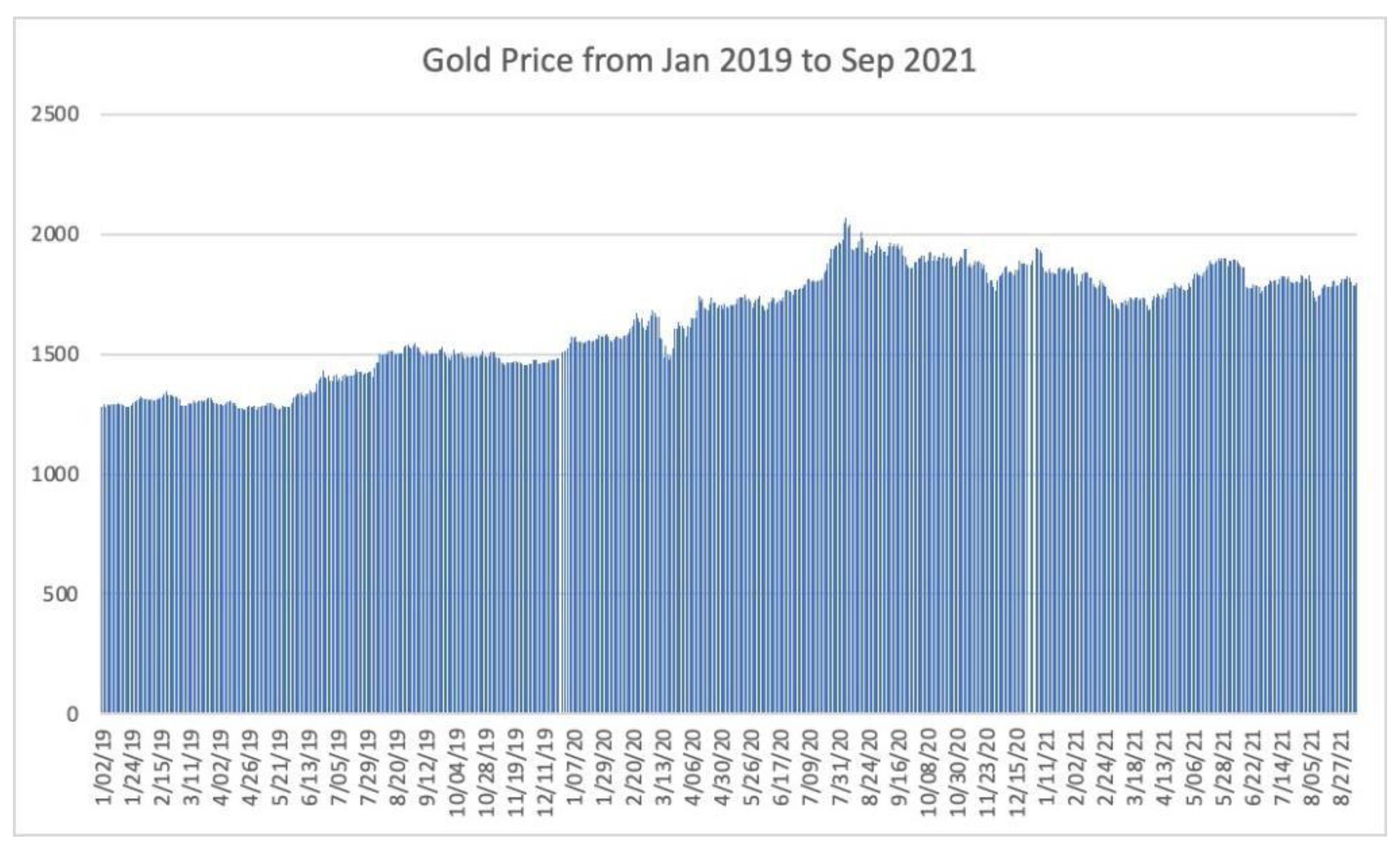
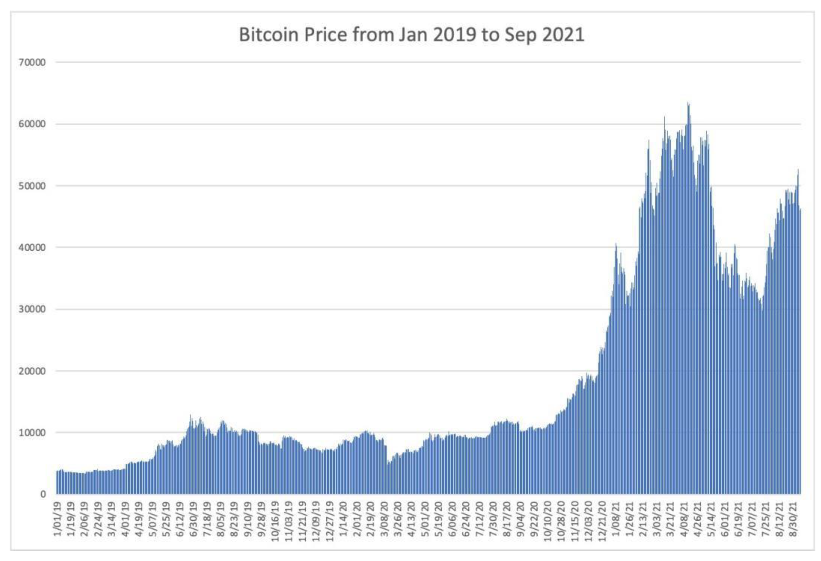
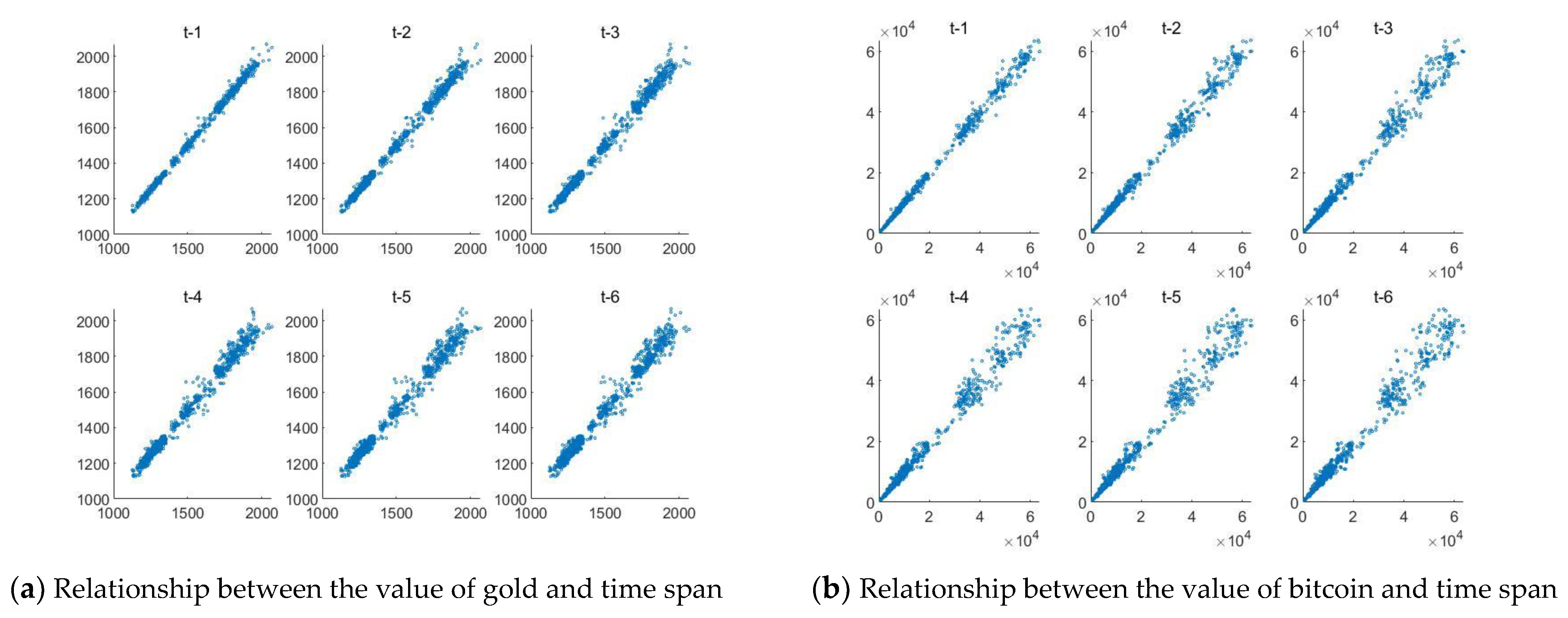
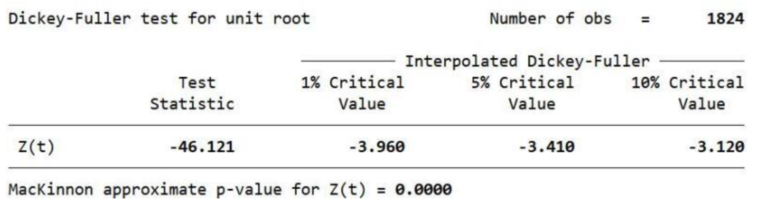
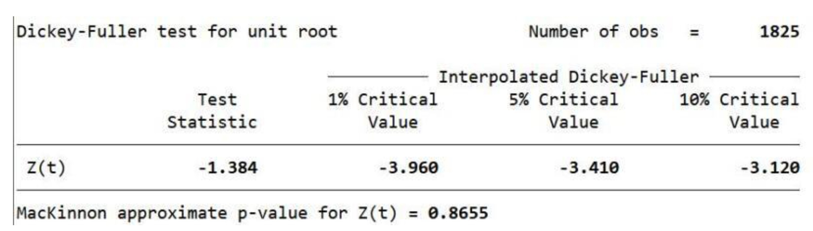
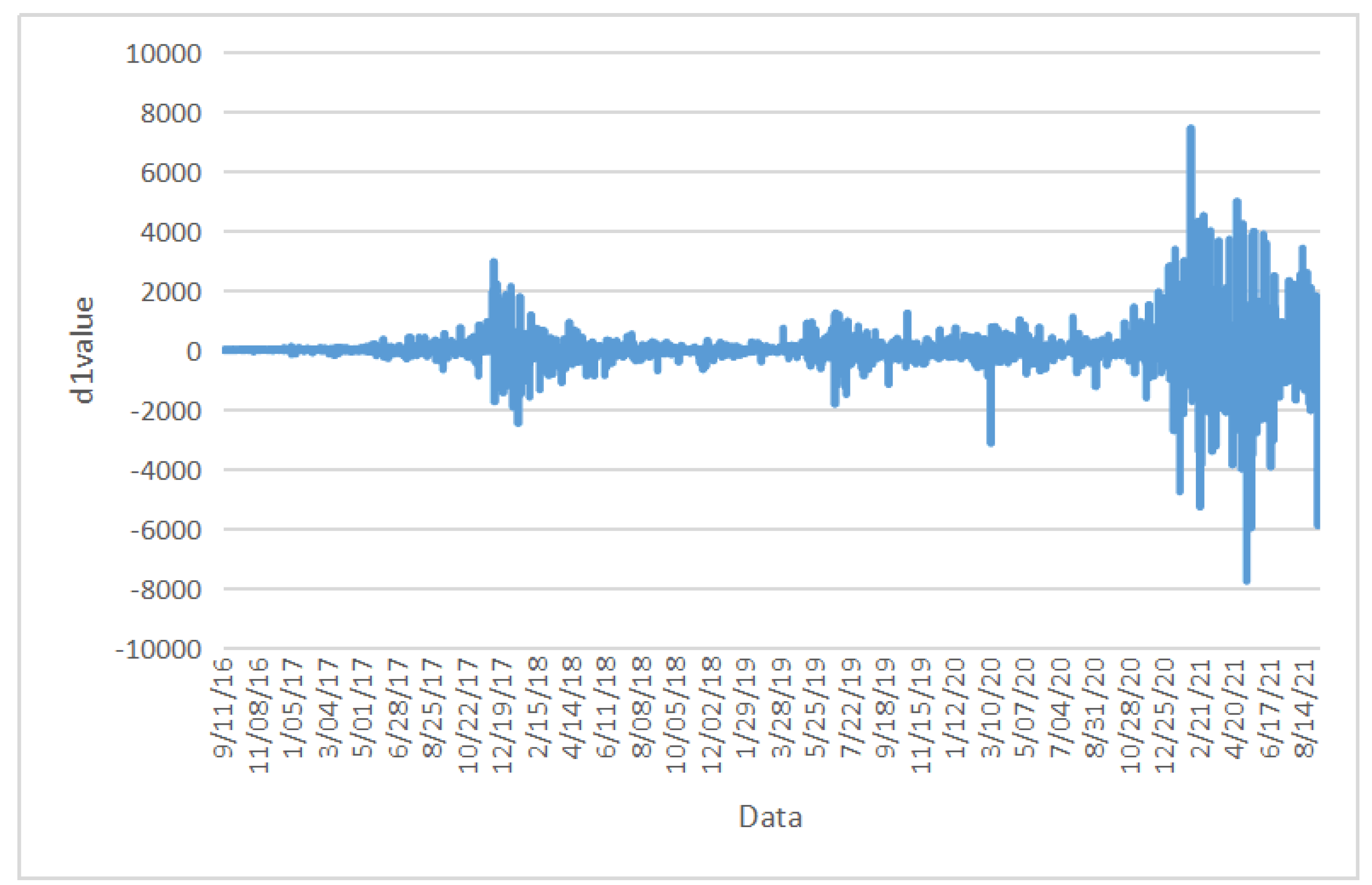
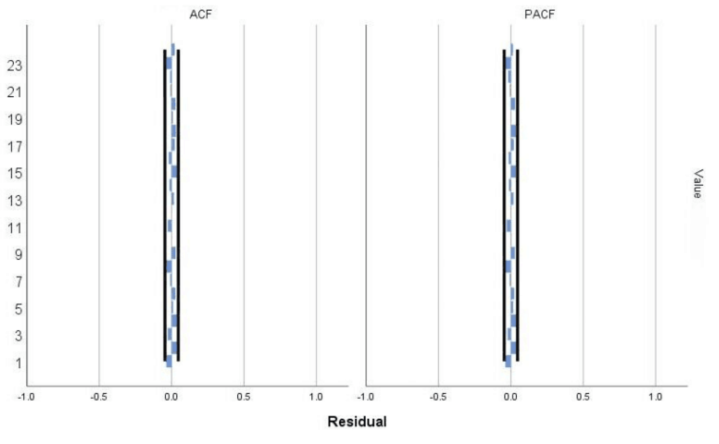
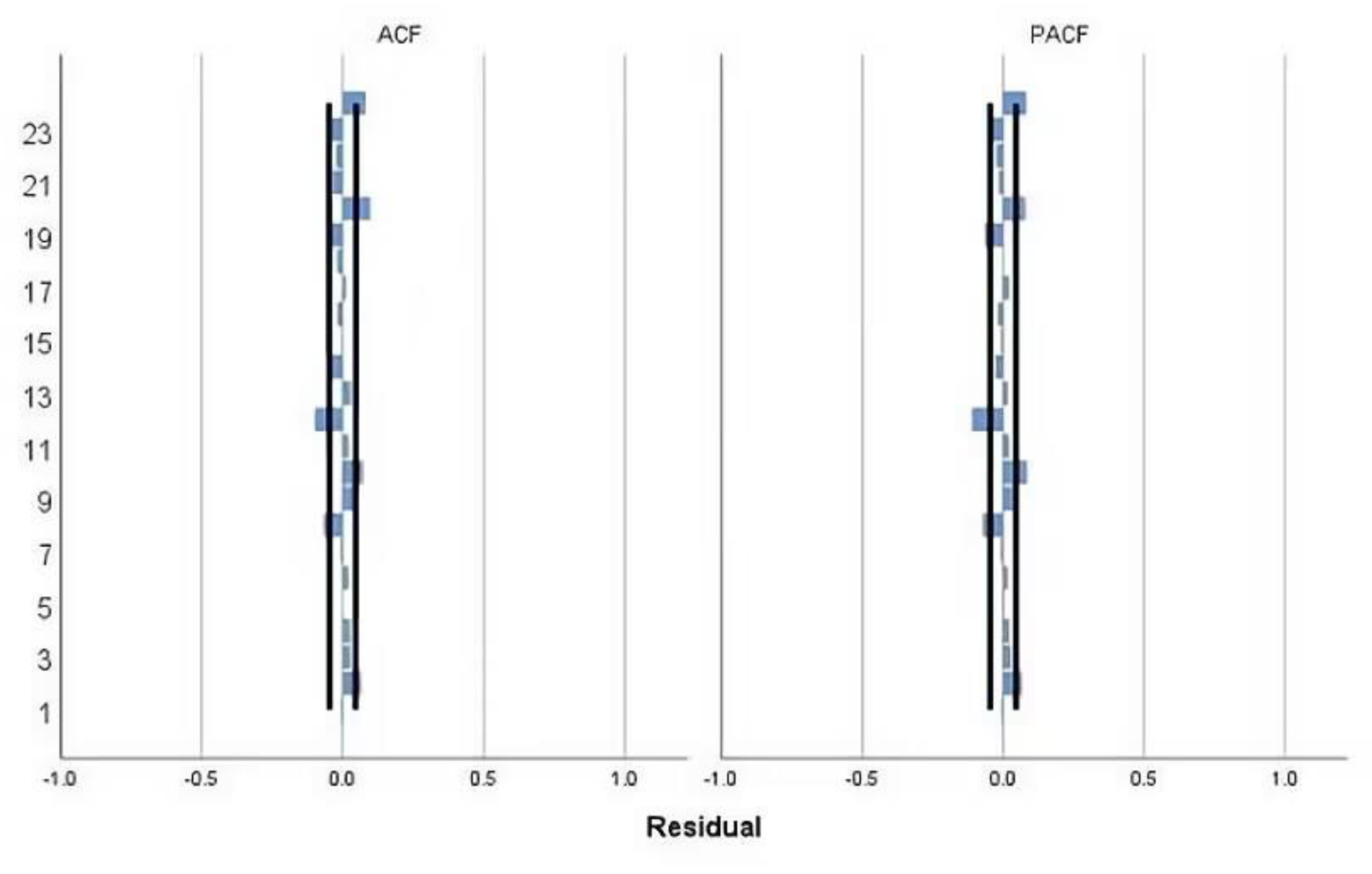
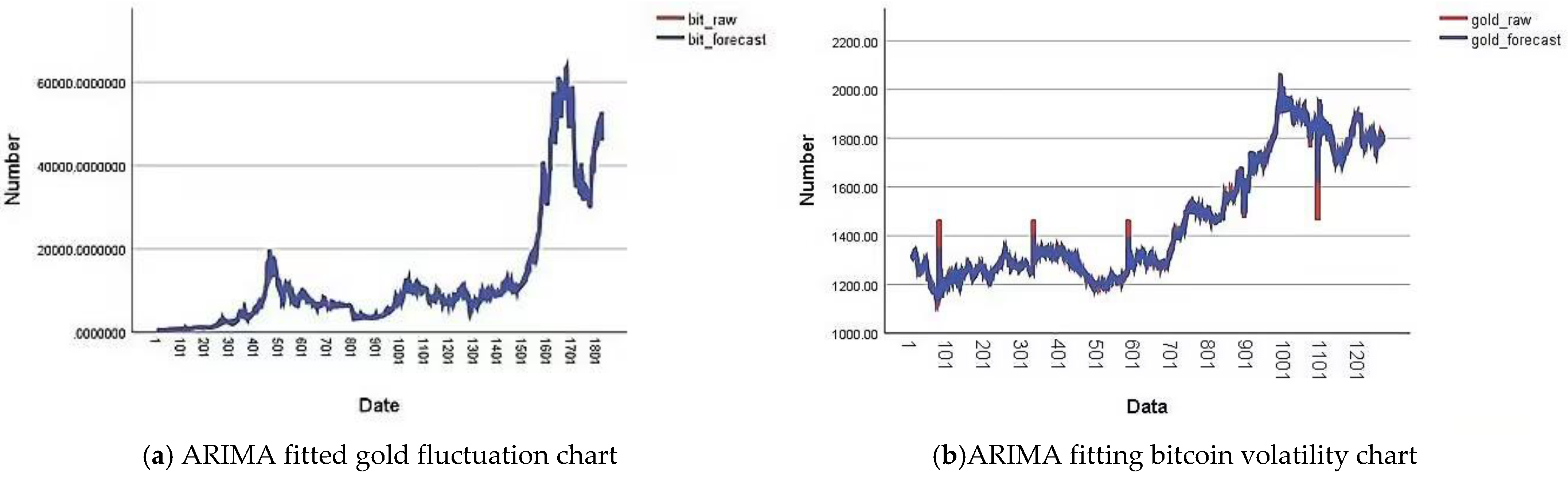
2.1.1. Settlement Price Forecast Analysis

Investors often predict future settlement prices based on past settlement price trends of financial products. However, it is not easy to predict the future price of bitcoin or gold with a high degree of accuracy; many volatile and non-smooth changes caused by unexpected factors make the settlement price of bitcoin or gold irregular. The correlation between gold (or bitcoin) and time is shown in Figure 3a,b. By looking at the settlement prices of bitcoin and gold from 9 November 2016, to 9 September 2021, we find that the prices of bitcoin and gold have very high volatility. Meanwhile, the future values of their settlement prices have a strong correlation with the past values, but their correlation gradually weakens with the increase of time interval, which indicates that their settlement prices are time series.

In the financial field, forecasting models for financial products such as stock prices often use neural networks or gray forecasting models [31], which have high accuracy and trend prediction but fail to consider the high volatility, time series, and time-varying nature of bitcoin and gold. Therefore, we should choose a time-series-based forecasting model to simulate the settlement prices of bitcoin and gold.

The correlation between bitcoin and gold is shown in Figure 4. Since the correlation between the settlement prices of bitcoin or gold changes over time, each additional variable becomes important each time the prediction model is re-estimated for the next step of forecasting, which marks the nature of non-linear studies, and since we find no correlation between the settlement prices of bitcoin and gold.

We use a single variable time-series model ARIMA and quadratic exponential smoothing for forecasting the settlement outcomes of bitcoin and gold, using a static forecasting approach that predicts the settlement price for the next day from price data up to that date and re-estimates the forecasting model for each step.

These two types of models not only consider the high volatility, time-varying, and time-series nature of the sample data but also are effective in making short-term forecasts that fit the characteristics of the frequent investments we make. In the following, we choose the daily settlement price of Bitcoin from 9 November 2016 to 9 September 2021 as an example to model and make short-term forecasts for its daily settlement price using the price data up to that date as a sample.

2.1.2. ARIMA (Autoregressive Integrated Moving Average Model)

We named the settlement price time series as P and performed DF smoothness test on P. The results are shown in Figure 5.

As can be seen from the figure, the statistic DF = −1.384, which is larger than the critical value at both the current confidence level of 1% and 5%, so the series is non-stationary and cannot be used directly, so we perform a first-order difference operation on it, and then perform a unit root test on the newly generated series, and the results are shown in Figure 6.

At this time, the statistic DF = −46.121, whose value is much smaller than the critical value at the current confidence level of 1%, 5%, and 10%, indicating that the original series has become smooth after the first-order difference. Figure 7 shows the first-order differential of the daily settlement price of bitcoin has smoothness. The rapid decay of the autocorrelation coefficient to zero in its autocorrelation plot also indicates that the first-order difference series is smooth, and the second-order difference test is no longer needed. Therefore d = 1, and the ARIMA (p,1,q) model can be established.

To fit and estimate the model, the bias correlation coefficient and autocorrelation coefficient and bias correlation coefficient are used to judge and select, and then the AIC criterion is used; that is, the smaller the obtained AIC value, the higher its accuracy and the better the fit, and the model is selected on merit. As the figure shows the first-order difference series autocorrelation plot (ACF) and partial autocorrelation function plot (PACF), it can be found that the autocorrelation coefficient and partial autocorrelation coefficient basically fall within the confidence interval, and both the autocorrelation plot and partial autocorrelation fall at K = 1 at the edge of the confidence band of two times the standard deviation, then p may take the value of 1 or 2. To further determine the model, compare the AIC test statistics of each model, and it is clear that the ARIMA(1,1,10) model is better than the other models, so the ARIMA(1,1,10) model is more appropriate for this series. Figure 8 shows the ARIMA model predicting performance.

In the next step, the ARIMA(1,1,10) model is used to predict the last 1 values of the time series, and the relative errors between the predicted and actual values are relatively small, less than 2%, thus indicating that the model has a good prediction effect, but at the same time, it can be seen that the relative error of the model prediction becomes larger as the prediction period increases. This shows that the model we constructed is effective and that the ARIMA model is more suitable for short-term forecasting and it is more accurate for short-term forecasting of bitcoin settlement price trends.

2.1.3. SESM (Second Exponential Smoothing Method)

The one-time exponential smoothing forecasting algorithm has the advantage of simplicity and fast operation, but when the movement of the sample series has an approximately linear trend, such as when the settlement price of bitcoin changes drastically due to external factors, forecasting using one-time exponential smoothing will introduce lagging bias. Therefore, it is usually possible to achieve more accurate forecasts by performing another smoothing process on top of the primary smoothing.

One-time exponential smoothing forecast equation:

$$S_t^{\left(1\right)}=a{x}_t+\left(1-\alpha \right)S_{t-1}^{\left(1\right)}-1$$

(1)

where: $S_t^{\left(1\right)}$, $S_{t-1}^{\left(1\right)}$ is the primary exponential smoothing value in period t, t − 1;$x_t$ is the actual value in period t; $\alpha$ is the smoothing factor: 0 < $\alpha$ < 1.

Forecasting using smoothed values, using the exponential smoothed value in period t as the forecast value in period t + 1, the model is

$$\begin{array}{l}{\widehat{x}}_{t+1}=S_t^{\left(1\right)}\\ {\widehat{x}}_{t+1}=\alpha x_t+\left(1+\alpha \right){\widehat{x}}_t\end{array}$$

(2)

The secondary exponential smoothing forecast is a smoothing forecast on top of the primary exponential smoothing forecast, calculated as follows.

$$\begin{array}{l}{S}_t^{\left(1\right)}=\alpha x_t+\left(1-\alpha \right)S_{t-1}^{\left(1\right)}\\ S_t^{\left(2\right)}=\alpha S_t^{\left(1\right)}+\left(1-\alpha \right)\end{array}$$

(3)

where $S_t^{\left(1\right)}$ is the primary exponential smoothing value, $S_t^{\left(2\right)}$ is the secondary exponential smoothing value, $x_t$ is the actual value in the t-th period, and $\alpha$ is the smoothing coefficient, 0 < $\alpha$ < 1.

Compute the parameters $a_t$, $b_t$ using exponential smoothing series,

$$\begin{array}{l}{a}_t=2S{t}^{\left(1\right)}-S{t}^{\left(2\right)}\\ b_t=\frac{\alpha }{1-\alpha }\left(S_t^{\left(1\right)}-S^{\left(2\right)}\right)\end{array}$$

(4)

Constructing predictive models:

$${\widehat{x}}_{t+m}=a_t+b_{t}m,m=1,2,\dots$$

(5)

${\widehat{x}}_{t+m}$ is the predicted value for the t + m th period.

To use the most suitable weighting coefficient $\alpha$ for the current sample data, the weighting coefficient $\alpha$ is increased from 0.05 to 0.95 in steps of 0.05, and the MSE (mean squared error) of different weighting coefficients is checked, and the weighting coefficient $\alpha$ with the smallest MSE is assigned to the quadratic exponential smoothing model at that time point to obtain the most accurate prediction value. Figure 9 shows the ACF and PACF that SESM has performed.

2.1.4. Comparison of the Accuracy of Prediction Models

Predictive models are evaluated based on the accuracy of their predictions. Here we evaluate the models using three metrics, MAPE (mean absolute error), RMSE (root mean square error total evaluation metric), and residuals, in three ways.

Through the forecasting data analysis of the sample data by the above three indicators (see Section 2.3 for details), the three ARIMA indicators are significantly better than the quadratic exponential smoothing model, so we choose ARIMA as the forecasting model for bitcoin and gold prices. The ARIMA model can not only consider the high volatility, time-varying, and time series of the sample data but also effectively make short-term forecasts, which is in line with our characteristics of making frequent investments.

Figure 10 shows the different performance between ARIMA and SESM. It can be concluded that ARIMA shows better performance than SESM.2.2.

2.2. Quantitative Trading Strategies Based on Dynamic Programming

2.2.1. Dynamic Planning Problem Analysis

After predicting the next day’s value through an accurate forecasting model, we further convert it into a growth rate and use it to develop a buy-sell-hold portfolio strategy. Here we use (C, G, B) to represent our daily portfolio, where C, G, and B are the amount of cash, gold, and bitcoin invested (in USD), respectively. Note that gold is only traded on weekdays when the market is open, so we designed the algorithm to ensure that the value of G is constant on days off. On weekdays, (C, G, B) will move funds according to the best combination ratio matched by the model. Initially, we considered a pure linear programming model. The objective function is:

$$MAX{Y}_t=W_G\ast R_G+W_B\ast R_B$$

(6)

However, the model has a major drawback, that is, with complete trust in the prediction results, funds will flood into the assets that are likely to increase in value soon, making the funds show a rapid rise in the model, but this behavior cannot exist in reality, because investors can realize the positive correlation between risk and return, and it is not desirable or scientific to frantically flood funds into an asset, so in order to make our model more realistic, we abandon the use of a pure linear programming model. The Algorithm 1 of asset investment has been show in the table below.

Algorithm 1 Simulation of asset investment

Input: original assets C, G, B, risk factor risk, data predicted from the original data, days to be invested, working days flag, growth rate of assets R. Output: the final distribution of the total value of assets V. 1: for t=1 to # of day do 2: if then 3:  allocate (data, asset table, risk) 4:  Calculate the optimal solution for asset allocation under risk for the three assets according to Date using the portfolio toolbox function to divide the funds Q 5:  G, B change amount for commission payment 6:  Evaluate the total value of C, G, B according to R 7: else 8:  Calculate the optimal solution for only two assets under risk according to Date, as above 9: end if 10: end for return V

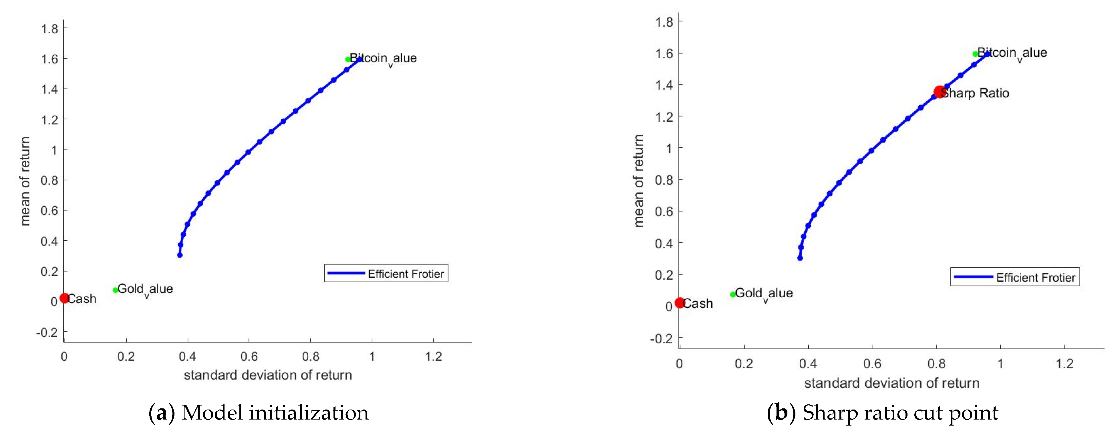
2.2.2. Mean-Variance Mode

In the actual investment process, investors need to measure the rate of return and consider the risk factor. So, in this paper, we introduce the concepts of the mean-variance model, Sharpe ratio, efficient frontier curve, etc. We consider an investor who owns three assets. Let the portfolio of three assets be p at timestamp t and the k-dimensional vector of asset returns of this portfolio be $X_t,t=1\dots n$. We ensure that the third-order nature of $X_t$ remains constant. The expected return and covariance matrix of the portfolio is denoted by ${\mu }_p$ and ${\sigma }_{p }$. The specific formulas are as follows.

$$\begin{gathered} r_p={\mathsf{\sum }}_{i=1}^n{\omega }_i{r}_i \\ {\mu }_p=E\left(r_p\right)=E\left({\mathsf{\sum }}_{i=1}^n{\omega }_i{r}_i\right) \\ {\sigma }^2=\mathrm{Var}\left(E\right(r_p\left)\right)=\mathrm{Var}{\left(E\right({\mathsf{\sum }}_{i=1}^n{\omega }_i{r}_i\left)\right)}^2 \\ {\sigma }_p^2=\pi r^2{\mathsf{\sum }}_i{\mathsf{\sum }}_j{\omega }_i{\omega }_j\mathrm{Cov}\left(r_i{r}_j\right) \end{gathered}$$

(7)

where $W_i$ is the weight of the assets in the portfolio, we have $W_1+\cdots +W_n=1$ (written in summation notation). That is, the assets are shared among the entire investor during the daily portfolio adjustment process.

According to Markovitz (1952), the weights of the optimal portfolio are found by minimizing the risk of the portfolio at a given level of expected return [32]. Figure 11 shows the cut point in frontier curves. The solution of the optimization problem leads to the set of optimal portfolios, which is called the efficient frontier. Figure 12 shows the efficient frontier after combining cash with risky assets.

However, in this paper, we match the optimal portfolio with different risks that the investor can bear as input values and the portfolio that maximizes the investment return at a given expected risk as output values.

So, we need to classify investors into three different types: aggressive, intermediate, and conservative, and the risk tolerance area is different for the three types of personalities. We set the risk tolerance of aggressive personalities at 0.7–0.9, intermediate personalities at 0.5–0.7, and conservative personalities at 0.3–0.5. By solving the model for different investor groups, we can derive the optimal asset portfolio for different groups of people and estimate and predict the future asset appreciation for different groups of people.

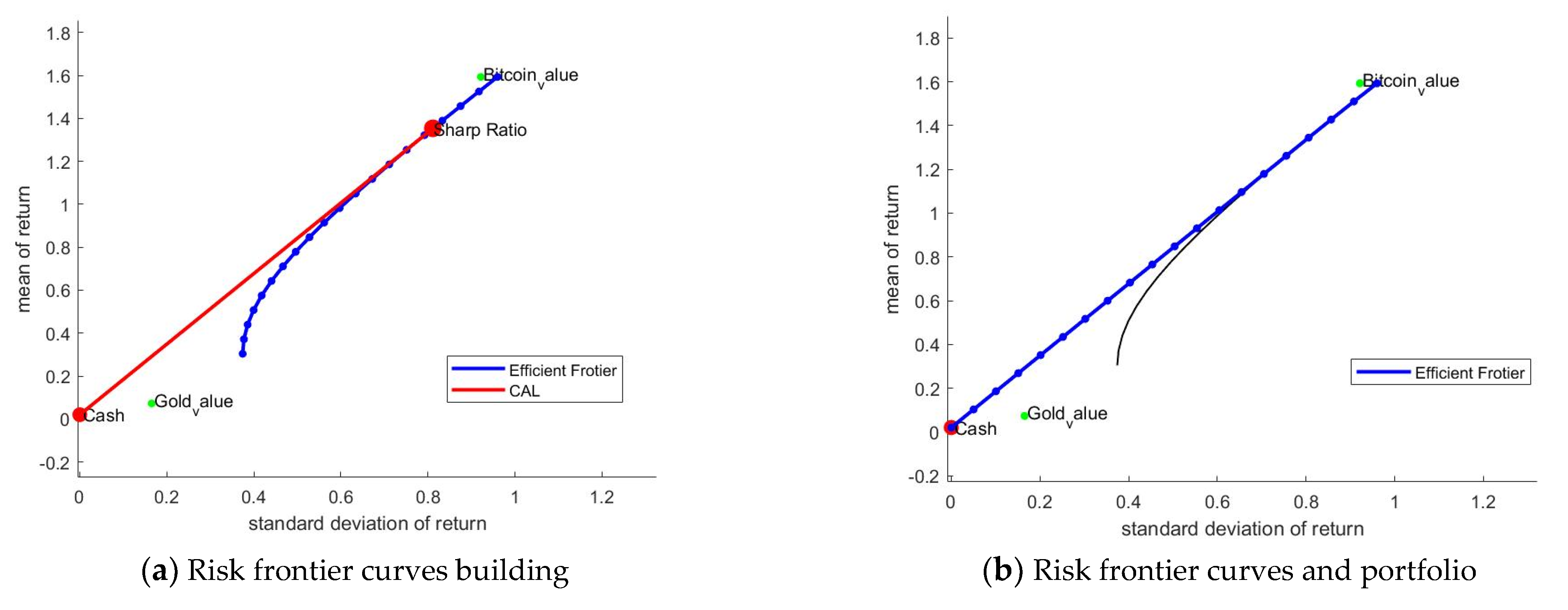
2.2.3. Combination of Effective Frontier and Sharpe Ratio

Merton (1972) proved that the efficient frontier in the mean-variance space is the upper part of the parabola [33].

We start with optimal portfolio planning for two risky assets, gold and bitcoin, and according to the theory proposed by Merton, we can derive an efficient frontier curve for the risky assets as shown in Figure 1, and the points on this efficient frontier curve have two characteristics:

• The point on the efficient frontier curve that maximizes the expected return for a given expected risk
• The point on the efficient frontier curve that minimizes risk given the expected return

However, this efficient frontier curve does not include the risk-free asset CASH, so to introduce the risk-free asset CASH into our portfolio, we introduce the concept of the Sharpe ratio. The Sharpe ratio captures the expected differential return per unit of risk associated with the differential return and considers the expected differential return between the two portfolios and the associated differential risk. The Sharpe ratio captures both risk and return. This is expressed as follows: an increase in return or a decrease in covariance (an increase in return and a decrease in risk) is considered a “good” event when the Sharpe ratio increases; a decrease in return or an increase in covariance (a decrease in return and an increase in risk) is considered a “bad” event when the Sharpe ratio decreases. In this case, the Sharpe ratio decreases [34]. Therefore, we hope that the higher the Sharpe ratio in the portfolio, the better. The formula for calculating the Sharpe ratio is as follows.

$$S{R}_p=\frac{E\left(r_p\right)-r_f}{{\sigma }_p}$$

(8)

The ex-ante Sharpe ratio is useful for decision-making (e.g., choosing an investment) because it gives an estimate of risk before the actual decision is made.

According to the Sharpe ratio formula, it can be learned that the slope of the line connecting the point on the efficient frontier curve of the risky asset to the point of the risk-free asset reflects the magnitude of the Sharpe ratio, and the slope is proportional to the Sharpe ratio. Thus, the objective is transformed from seeking the maximum Sharpe ratio to the maximum slope of the line between the point on the effective frontier curve of the risky asset and the point on the risk-free asset. Based on the graph, we know that the Sharpe ratio is maximized when the line is tangent to the efficient frontier curve [34], i.e., the optimal portfolio is achieved. This is shown in Figure 13. Ultimately, Figure 13 reflects the new efficient frontier curve after adding the risk-free assets, and each point on the line represents an optimal portfolio.

Eventually, the data is substituted into the established model. As shown in

Table 1. The ultimate return of different personalities.

	Aggressive	Intermediate	Conservative
Return	15,581.85	9869.34	3676.75

, after calculation, the initial $1000 will have different final returns under different investment personalities. Here, we set the maximum risk tolerance for the aggressive personality at 0.8, the maximum risk tolerance for the intermediate personality at 0.6, and the maximum risk tolerance for the conservative personality at 0.3.

The results are as follows: Aggressive investor ends up with 15,581.85 USD, Intermediate investor ends up with 8869.34 USD, and Conservative investor ends up with 3676.75 USD.

2.3. Analysis of the Advantages and Disadvantages of Prediction Models

Based on the known daily settlement prices of gold and bitcoin from September 2016 to September 2021, we apply ARIMA and quadratic exponential smoothing to forecast them, respectively, and we find that both forecasting methods can obtain more accurate forecasting data, and their forecasting curves almost overlap with the real values. To compare the advantages and disadvantages of the two forecasting methods more accurately, here we introduce three indicators such as MAPE (mean absolute error), RMSE (root mean square error), and residuals, to compare the errors of the two forecasting models with the actual values.

Table 2. The table comparing ARIMA with RMSE.

	MAPE	RMSE
ARIMA	0.026754	651,580.6
SEME	0.034827	742,891.6

shows that the ARIMA model is significantly better than the quadratic exponential smoothing model, and at the same time, the fit of the ARIMA model reaches 99.7%, which is already very close to the real data, indicating that it has very good prediction accuracy.

3. Improvement of the Optimization of the Model

3.1. Planning Strategy Model Improvement

3.1.1. Optimization of Sharpe Ratio

Since the assumed return of the traditional Sharpe ratio is not correlated with the rest of our portfolio. This is because when one of the assets is correlated with the rest, it affects the Sharpe ratio judgment. For example, when bitcoin has a lower Sharpe ratio than gold, the Sharpe ratio would guide us to choose gold over bitcoin. However, if bitcoin’s return is negatively correlated with the portion of our portfolio and gold’s return is positively correlated with our portfolio, then buying bitcoin will reduce the risk of the portfolio, while buying gold will increase the risk, and if we consider the riskiness, we may choose bitcoin over gold, which contradicts the judgment we made through the traditional Sharpe ratio [35]. We find that gold has a correlation of 0.68 with bitcoin in the current sample data.

$$R_A\ge R_p^{old}+\left[\frac{{\sigma }_{R_p}^{new}}{{\sigma }_{R_p}^{old}}-1\right]\frac{R_p^{old}}{a}$$

(9)

To solve this problem, we introduce the generalized Sharpe ratio with the following formula by constructing two Sharpe ratios, one for the current portfolio as a whole and the other for the new portfolio, and we choose the new portfolio if the Sharpe ratio of the new portfolio is higher than the Sharpe ratio of the old portfolio. Here, we bring the generalized Sharpe ratio into the planning model to derive the locally optimal solution for the current situation.

3.1.2. Particle Swarm Optimization Algorithm

Particle Swarm Optimization (PSO) is an intelligent optimization method that simulates the mechanism of cooperation in the foraging behavior of animal groups in the biological world to find the optimal solution to the problem for the population. The algorithm has a simple principle, is easy to implement, and has fewer control parameters. Firstly, the PSO algorithm initializes to generate a group of random particles with no volume and no mass, each particle has a displacement term and a velocity term, and each particle can be treated as a feasible solution, while the real good feasible solution must be determined by the fitness function.

Assume that the PSO algorithm searches in D-dimensional space and is a population of m particles. Each particle maintains two vectors in the evolution process, the velocity vector$V_i=\left(v_{i1},v_{i2},\dots ,v_{iD}\right)$ and the position vector $X_i=\left(x_{i1},x_{i2},\dots ,x_{iD}\right)$. The current searched individual optimal position is $p_i^t=\left(p_{i1}^t,p_{i2}^t,\dots ,p_{iD}^t\right)$ and the global optimal position is $P_g^t=\left(p_{g1}^t,p_{g2}^t,\dots ,p_g^{t}D\right)$, where $i=1,2,\dots ,m$.

For each particle $i$, the velocity and position in the dth dimension are updated according to the following equation:

$$v_{id}^{t+1}=w{v}_{id}^t+c_1{r}_1\left(p_{id}-x_{id}^t\right)+c_2{r}_2\left(p_{gd}-x_{id}^t\right)$$

(10)

$$x_{id}^{t+1}=x_{id}^t+v_{id}^{t+1}$$

(11)

where: t is the number of current iterations, w is the inertia weight, $r_1$, $r_2$ are the random numbers between [0,1].

The speed and direction of motion of each particle determine the next position of the particle and the historical optimal solution found by the particle itself so far and the historical optimal solution found by the whole population influence the speed and direction of motion of each particle next time, and each particle is regarded as a feasible solution of the objective function, and the position value of the particle is brought into the fitness function to calculate and evaluate the goodness of the solution. Finally, the global optimal solution is obtained.

3.1.3. Model Stability Testing

Combining each predicted value and replanning, our model makes the optimal strategy for that riskiness on the same day, resulting in the highest expectation. To prove that our planning model is arriving at the best strategy, we add certain perturbation terms to the best planning model. If the perturbed return expectations are all less than our maximum expectation, it means that our model does the best planning. Here, we adjust the original best model every 10 days, and eventually, we can find that the expected returns of the perturbed model are all lower than our original plan, which indicates that our original plan is a local optimal solution.

4. Stability Analysis of the Model

This question considers how the expected return, the number of trades in gold, and the number of trades in bitcoin change when the optimal portfolio strategy we solved for in Problem 1 changes in transaction costs. However, we also consider that different transaction cost rates may have different effects on expected return, number of trades in gold, and number of trades in bitcoin when facing different investment personalities. Thus, we conducted separate analyses on the impact of transaction costs for aggressive, intermediate, and conservative personalities. We set the risk tolerance index to 0.8 for the aggressive personality, 0.6 for the intermediate personality, and 0.3 for the conservative personality, respectively.

In the table, ratio_gold and ratio_bitcoin denote the percentage of fees for gold and bitcoin, respectively; return denotes the final benefit, g_times denotes the number of gold transactions, and b_times denotes the number of bitcoin transactions.

From

Table 3. The table of different personalities under the influence of different rates.

Aggressive	1	2	3	4	5	6	7
ratio_gold	1%	1.50%	0.50%	1%	1%	0.50%	2%
ratio_bitcoin	2%	2%	2%	1.50%	2.50%	1%	4%
return	15,581	15,181	15,992	19,051	12,740	23,901	6599
g_times	1189	1176	1297	1218	1214	1362	1183
b_times	1372	1302	1452	1414	1289	1501	1275
Intermediate
return	8869	8636	9108	10,427	7542	12,589	4395
g_times	378	314	498	354	318	458	245
b_times	923	892	956	1136	893	1013	769
Conservative
return	3676	3632	3721	3939	3431	4272	2722
g_times	112	59	248	126	102	272	53
b_times	654	631	642	712	521	852	383

, we can see that as the transaction fee of an asset increases, the number of transactions of that asset becomes significantly lower, which leads to a significant decrease in the value of the optimal asset portfolio. On the other hand, as the transaction fee for an asset decreases, the number of transactions for that asset increases significantly, resulting in a significant increase in the value of the optimal portfolio.

Moreover, we measure the impact of the change in transaction costs on different personalities by calculating the variance of the number of transactions corresponding to different personalities. It can be easily seen that the variance of both g_times and b_times for the aggressive personality is the smallest, followed by the middle personality, and the variance of g_times and b_times for the conservative personality is the largest. This suggests that: for relatively conservative investors, the increase in trading fees causes them to substantially adjust their number of trades, thus showing large volatility in the number of trades. For the relatively aggressive investors, the increase in trading fees does not deter them from trading to a large extent, so they show less volatility in the number of trades.

5. Model Evaluation

5.1. Strength

In this study, we propose an investor personality-based investment strategy model, which is a mixture of a forecasting model and an economic portfolio model. Compared to other studies, this study has the following advantages.

• Comprehensive consideration:

In solving for the optimal asset portfolio allocation, we consider investor personality factors, namely: aggressive, intermediate, and conservative. Aggressive personalities can withstand relatively high risk in pursuit of greater investment returns. Conservative personalities usually avoid risk, making investment returns protected. Therefore, for different types of investors, the model proposes different investment portfolio options and indicates the investment risks.

• Making the best use of information:

We fully used the data from the two tables given in the question for the training of the ARIMA model and performed data cleaning with SQL Server.

• Excellent robustness of the model:

Our model is robust, indicating that small changes in parameters do not lead to large differences in results. By substituting different fee rates, all ensure that the fees are apportioned to cash, gold, and bitcoin in a certain percentage, ensuring that the combination of cash, gold, and bitcoin remains the optimal portfolio allocation.

• Low time complexity:

By introducing the particle swarm algorithm, we make the calculation process of the optimal asset mix ratio optimized, which greatly improves the speed of computing.

• Improvements in data processing:

Using SQL Server to flag weekdays and days off in GOLD data with “flags” allows us to identify the freeze period of gold when making portfolio allocations quickly and accurately.

5.2. Weakness

Although the methodology of this paper proves its advantages in the portfolio field compared to the classical model, a review of previous studies shows that the above hybrid model has some drawbacks.

• Insufficient data:

You need to wait for at least one month before you can predict the market value of the next day based on the market value movement of this month, and the waiting time will cause a decrease in the final return.

• Subjective assumptions about personality:

We have used only the maximum risk that the investor can bear as the basis for judging personality, which is somewhat subjective.

6. Conclusions

In the world’s financial markets, there are various types of investments, such as gold, bitcoin, and stocks. Among them, gold and bitcoin have an extremely important position in the financial market as part of the capital market. It is well known that the gold and bitcoin markets have huge money-making benefits, and accurate predictions of the value of the financial markets represent an increasing profit for investors. Therefore, predictive analysis of capital markets has become a trend in the modern financial world. Nowadays, as the wave of artificial intelligence is sweeping the world, machine learning algorithms have been widely used in the field of financial investment as a key technology to achieve artificial intelligence. In this paper, we use machine learning algorithms combined with knowledge of finance to consider risks and maximize returns to solve the problem of optimal allocation of financial investments.

For this proposed optimal asset investment matching problem, we break it down into a prediction problem and a dynamic planning problem. In the prediction problem, we use the historical data of the value up to that date to predict the future value. Based on the time-series characteristics of the data, we measure the forecasting effectiveness by comparing the forecasting effectiveness of ARIMA and quadratic exponential smoothing models with three indicators: MAPE, RMSE, and residuals. Finally, the ARIMA model with a better prediction effect was chosen as our prediction model. In the dynamic programming problem, we recognize that any investor would like to maximize the return on investment, but the return is positively correlated with the risk. So, in this subproblem, we introduce the theory of the mean-variance model, Sharpe ratio, and efficient frontier to find the equilibrium point of risk and return.

However, the traditional Sharpe ratio cannot overcome the shortcomings due to asset correlation, so we introduce the concept of generalized Sharpe ratio and combine the Sharpe ratio with the efficient frontier and add the particle swarm algorithm to speed up the convergence. After the model is built, we divide the investment population into three categories: aggressive, intermediate, and conservative, and personalize the analysis for each of the three different investment populations to derive the best portfolio solution for each of the different populations and finally derive the total value after five years.

Then, we record the final return, the number of gold transactions, and the number of bitcoin transactions under the optimal investment scheme by changing the fee rate. Ultimately, we interpret the data from two perspectives. Horizontally, the number of trades for a given asset decreases as the fees for buying and selling that asset increase, which in turn decreases the final return, i.e., the number of trades for an asset is negatively correlated with the fees for that asset. Longitudinally, we find that investors with aggressive personalities adopt strategies that are least sensitive to transaction costs, while investors with conservative personalities are the most sensitive. This means that transaction costs do not dilute the investment enthusiasm of aggressive investors but can largely influence the investment decisions of conservative investors.

7. Future Research Direction

Future research is needed to determine the performance of the proposed model in European or Asian stock markets. Other machine learning models, such as deep reinforcement learning (DRL), transformer, etc., should be used and compared with the proposed ARIMA model. More exogenous variables should be applied in future research; for example, the behavior of the decision game between investors in the stock market can be further simulated by introducing a multi-party evolutionary game model. Another future direction would be to use the hybrid model to test and validate the investment scenarios for several fiscal years. Research indicators such as quantitative investor investment rationality can be analyzed in the broader context of regional stock exchange markets.

References

1. Kannan, K.S.; Sekar, P.S.; Sathik, M.; Arumugam, P. Financial stock market forecast using data mining techniques. Proc. Int. Multiconference Eng. Comput. Sci. 2010, 1, 4. [Google Scholar]
2. Tyson, E. Investing for Dummies, 6th ed.; John Wiley & Sons: Hoboken, NJ, USA, 2011. [Google Scholar]
3. Mulyadi, M.S.; Anwar, Y.; Khalid, K.; Shawa, K.C.; Singh, G.; Ashraf, S.W.A. Gold versus stock investment: An econometric analysis. Int. J. Dev. Sustain. 2012, 1, 1–7. [Google Scholar]
4. Ibrahim, M.H. Financial market risk and gold investment in an emerging market: The case of Malaysia. Int. J. Islam. Middle East. Financ. Manag. 2012, 4, 79–89. [Google Scholar]
5. Selgin, G. Synthetic commodity money. J. Financ. Stab. 2015, 17, 92–99. [Google Scholar]
6. Popper, N. Digital gold: Bitcoin and the inside story of the misfits and millionaires trying to reinvent money. HarperCollins 2016. [Google Scholar]
7. Yenidoğan, I.; Çayir, A.; Kozan, O.; Dağ, T.; Arslan, Ç. Bitcoin forecasting using ARIMA and PROPHET. In Proceedings of the 3rd international conference on computer science and engineering (UBMK), Sarajevo, Bosnia and Herzegovina, 20–23 September 2018; pp. 621–624. [Google Scholar]
8. Brusov, P.; Filatova, T.; Chang, S.I.; Lin, G. Innovative investment models with frequent payments of tax on income and of interest on debt. Mathematics 2021, 9.13, 1491. [Google Scholar]
9. Romigh, G.D.; Brungart, D.S.; Simpson, B.D. Free-field localization performance with a head-tracked virtual auditory display. IEEE J. Sel. Top. Signal Process. 2015, 9.5, 943–954. [Google Scholar]
10. Zhang, L.; Aggarwal, C.; Qi, G.-J. Stock price prediction via discovering multi-frequency trading patterns. In Proceedings of the 23rd ACM SIGKDD International Conference on Knowledge Discovery and Data Mining, Halifax, NS, Canada, 13–17 August 2017. [Google Scholar]
11. Brown, K.; Harlow, W.; Zhang, H. Investment Style Volatility and Mutual Fund Performance. J. Investig. Manag. 2021, 19, 78. [Google Scholar]
12. Cakici, N.; Zaremba, A. Size, Value, Profitability, and Investment Effects in International Stock Returns: Are They Really There? J. Investig. 2021, 30, 65–86. [Google Scholar]
13. Brusov, P.; Filatova, T. The Modigliani–Miller theory with arbitrary frequency of payment of tax on profit. Mathematics 2021, 9, 1198. [Google Scholar]
14. Modigliani, F.; Miller, M. The cost of capital, corporate finance, and the theory of investment. Am. Econ. Rev. 1958, 48, 261–297. [Google Scholar]
15. Modigliani, F.; Miller, M. Corporate income taxes and the cost of capital: A correction. Am. Econ. Rev. 1963, 53, 147–175. [Google Scholar]
16. Modigliani, F.; Miller, M. Some estimates of the cost of capital to the electric utility industry 1954–1957. Am. Econ. Rev. 1966, 56, 333–391. [Google Scholar]
17. Black, F.; Litterman, R. Global Portfolio Optimization.Financ. Anal. J. 1992, 48, 28–43. [Google Scholar]
18. Filatova, T.; Brusov, P.; Orekhova, N. Impact of advance payments of tax on profit on effectiveness of investments. Mathematics 2022, 10.4, 666. [Google Scholar]
19. Zolfaghari, M.; Gholami, S. A hybrid approach of adaptive wavelet transform, long short-term memory and ARIMA-GARCH family models for the stock index prediction. Expert Syst. Appl. 2021, 182, 115149. [Google Scholar]
20. Voulodimos, A.; Nikolaos, D.; Anastasios, D.; Eftychios, P. Deep learning for computer vision: A brief review. Comput. Intell. Neurosci. 2018, 2018, 7068349. [Google Scholar]
21. Rubesam, A. Machine learning portfolios with equal risk contributions: Evidence from the Brazilian market. Emerg. Mark. Rev. 2022, 51, 100891. [Google Scholar]
22. Wickham, H. ggplot2: Elegant Graphics for Data Analysis, 2nd ed.; Springer: Berlin/Heidelberg, Germany, 2016. [Google Scholar]
23. Dospinescu, O.; Dospinescu, N. A profitability regression model of Romanian stock exchange’s energy companies. In Proceedings of the 17th International Conference on Informatics in Economy Education, Research & Business Technologies, Iasi, Romania, 17–20 May 2018. [Google Scholar]
24. Brusov, P.; Filatova, T.; Orekhova, N.; Eskindarov, M. Modern Corporate Finance, Investments, Taxation and Ratings; Springer International Publishing: Berlin/Heidelberg, Germany, 2018. [Google Scholar]
25. Du, Y. Application and analysis of forecasting stock price index based on combination of ARIMA model and BP neural network. In Proceedings of the 2018 Chinese Control and Decision Conference (CCDC), Shenyang, China, 9–11 June 2018. [Google Scholar]
26. Garlapati, A.; Krishna, D.R.; Garlapati, K.; Yaswanth, N.m.S.; Rahul, U.; Narayanan, G. Stock Price Prediction Using Facebook Prophet and Arima Models. In Proceedings of the 2021 6th International Conference for Convergence in Technology (I2CT), Maharashtra, India, 2–4 April 2021. [Google Scholar]
27. Huang, K.Y.; Jane, C.J. A hybrid model for stock market forecasting and portfolio selection based on ARX, grey system and RS theories. Expert Syst. Appl. 2009, 36.3, 5387–5392. [Google Scholar]
28. Sadorsky, P. Forecasting solar stock prices using tree-based machine learning classification: How important are silver prices? N. Am. J. Econ. Financ. 2022, 61, 101705. [Google Scholar]
29. Stosic, D.; Stosic, D.; Ludermir, T.B.; Stosic, T. Collective behavior of cryptocurrency price changes. Phys. A: Stat. Mech. Appl. 2018, 507, 499–509. [Google Scholar]
30. Jain, P.; Jain, S. Can machine learning-based portfolios outperform traditional risk-based portfolios? The need to account for covariance misspecification. Risks 2019, 7, 74. [Google Scholar]
31. Wang, G.; Wang, X.; Wang, Z.; Ma, C.; Song, Z. A VMD–CISSA–LSSVM Based Electricity Load Forecasting Model. Mathematics 2022, 10, 28. [Google Scholar]
32. Munim, Z.H.; Shakil, M.H.; Alon, I. Next-day bitcoin price forecast. J. Risk Financ. Manag. 2019, 12, 103. [Google Scholar]
33. Maller, R.A.; Durand, R.B.; Jafarpour, H. Optimal portfolio choice using the maximum Sharpe ratio. J. Risk 2010, 12, 49. [Google Scholar]
34. Bodnar, T.; Schmid, W. Econometrical analysis of the sample efficient frontier. Eur. J. Financ. 2009, 15, 317–335. [Google Scholar]
35. Wang, Y.; Yuankai, G. Forecasting method of stock market volatility in time series data based on mixed model of ARIMA and XGBoost. China Commun. 2020, 17, 205–221. [Google Scholar]
Figure 1. Gold prices from January 2019 to September 2021.
Symmetry 14 02292 g001
Figure 2. Bitcoin price from January 2019 to September 2021.
Symmetry 14 02292 g002
Figure 3. The correlation between gold and bitcoin and time.
Symmetry 14 02292 g003
Figure 4. Correlation test between bitcoin and gold.
Symmetry 14 02292 g004
Figure 5. Smoothing test for daily settlement price of bitcoin.
Symmetry 14 02292 g005
Figure 6. Smoothing test for the first-order difference of the daily settlement price of bitcoin.
Symmetry 14 02292 g006
Figure 7. The first-order differential of the daily settlement price of bitcoin has smoothness.
Symmetry 14 02292 g007
Figure 8. ARIMA-based ACF and PACF images of Bitcoin.
Symmetry 14 02292 g008
Figure 9. SESM-based ACF and PACF images of Bitcoin.
Symmetry 14 02292 g009
Figure 10. Comparison of Gold and Bitcoin prediction data and actual data derived using ARIMA.
Symmetry 14 02292 g010
Figure 11. Risk frontier curves and their cut points.
Symmetry 14 02292 g011
Figure 12. Combining cash with risky assets and adding cash as a risk-free asset to the adjusted risk frontier curve.
Symmetry 14 02292 g012
Figure 13. Allocation percentages of each asset under different risks.
Symmetry 14 02292 g013