Certain Operations on Picture Fuzzy Graph with Application

Abstract

Fuzzy graphs (FGs) can play a useful role in natural and human-made structures, including process dynamics in physical, biological, and social systems. Since issues in everyday life are often uncertain due to inconsistent and ambiguous information, it is extremely difficult for an expert to model those difficulties using an FG. Indeterminate and inconsistent information related to real-valued problems can be studied through a picture of the fuzzy graph (PFG), while the FG does not provide mathematically acceptable information. In this regard, we are interested in reducing the limitations of FGs by introducing some new definitions and results for the PFG. This paper aims to describe and explore a few properties of PFGs, including the maximal product (MP), symmetric difference (SD), rejection (RJ), and residue product (RP). Furthermore, we also discuss the degree and total degree of nodes in a PFG. This study also demonstrates the application of a PFG in digital marketing and social networking.

1. Introduction

In 1965, Zadeh [1] presented the fuzzy set (FS) as an extension of the crisp set to deal with imprecise and unclear information in ambiguous situations, and it is effective and acceptable. It can be characterized by a true membership function similar to a probability function having ranges in [0, 1]. These concepts successfully depict complicated events that cannot be adequately stated using classical mathematics and are also useful to understand approximate reasoning problems. Rosenfeld [2] studied various fuzzy graph-theoretical ideas such as cycles, connectedness, and path. The FG has many applications in topological space and algebra, among other areas. Bhattacharya [3] discussed the association of the fuzzy group with fuzzy graphs. Bhutani [4] worked on automorphism in FGs. Gani and Latha [5] introduced the irregularity of FGs. Gani and Ahmad [6] defined the degree and size of FGs. Morderson and Peng [7] defined the join, Cartesian product, union, and composition of fuzzy subgraphs of graphs. Mathew and Sunitha [8] discussed the basic applications of FGs. It is not necessarily true that the membership degree is 1, as non-membership degrees also exist, and indeterminacy occurs in an intuitionistic fuzzy set. Shao et al. [9] described new concepts of the bondage number in the intuitionistic fuzzy graph (IFG). Rashmanlou et al. [10,11,12] studied a bipolar fuzzy graph. Rashmanlou et al. [13,14,15,16] also studied interval-valued fuzzy graphs. Gulzar et al. [17] described the novel application of a complex intuitionistic fuzzy set. Gulzar et al. [18] worked on the class of the t-intuitionistic fuzzy subgroup. Bhunia [19] briefly studied the algebraic characteristics of fuzzy sub-e-group. Smarandache [20] introduced the theory of the neutrosophic set involving indeterminacy and inconsistent data. Hassan and Malik [21] presented the classification of the bipolar single-valued neutrosophic graph.

Zuo et al. [22] introduced the idea of the PFG. Some operations on PFGs, namely, Cartesian product, composition, join, lexicographic product, strong product, and direct product, are discussed. The PFG is a generalization of the FG and IFG. The PFG is an efficient tool to handle uncertain issues in everyday life, in which an IFG may not provide exact answers. A PFG is very helpful in addressing uncertain problems that consist of multiple answers, such as no, yes, refusal, and abstain.

The main contributions of this paper are as follows:

• In this study, we establish some new properties of the PFG, including MP, SD, RP, and RJ, which may be suggestive of some aspects of network design because it contains the additional neutral grade, while the FG and IFG may fail in networking due to lack of information.
• We explore some of the properties of the resultant picture fuzzy graphs, especially the degree of vertices and total degree as a modification, acquired from the given picture fuzzy graphs using these operations.
• The picture fuzzy graph is more adaptive and generalized than the FG and IFG. The application of picture fuzzy graphs is widely applicable in networking and enables solving three-dimensional problems. We apply the concept of picture fuzzy graphs to a decision-making problem.

The layout of this paper is as follows:

We describe a few fundamental notions in Section 2 that are helpful for understanding this paper. Section 3 presents a few properties of the PFG, including MP, SD, RP, and RJ. We define the degree of a vertex and the total degree of a vertex with examples. In Section 4, we describe the application of a PFG in networking. Finally, we provide concluding remarks and some future directions in Section 5.

2. Preliminaries

This section involves some basic definitions. We recall some important definitions and discuss them in depth to illustrate the notion of the vertex degree. The symbols ∨ and ∧ represent max and min, respectively.

Definition 1

([22]). Picture fuzzy set (PFS) is defined as:

$$\begin{array}{c}\hfill U=<p:{\chi }_U\left(p\right),{\varphi }_U\left(p\right),{\psi }_U\left(p\right),p\in X>\end{array}$$

which follows:

$$\begin{array}{c}\hfill 0\le {\chi }_U\left(p\right)+{\varphi }_U\left(p\right)+{\psi }_U\left(p\right)\le 1\end{array}$$

where ${\chi }_U:V\to [0,1]$ represents the degree of the true membership function, ${\varphi }_U:V\to [0,1]$ represents the degree of the neutral membership function, and ${\psi }_U:V\to [0,1]$ represents the degree of the falsity membership function.

The refusal membership degree is defined as follows:

$$\begin{array}{c}\hfill {\pi }_U\left(p\right)=1-{\chi }_U\left(p\right)+{\varphi }_U\left(p\right)+{\psi }_U\left(p\right)\end{array}$$

Definition 2

([22]). A PFG on a non-empty set V is a pair $\mathbb{G}=(U,W)$, where U is a picture fuzzy set on V, and W is a picture fuzzy relation on V. It is expressed as follows:

$$\begin{array}{c}\hfill {\chi }_W\left(pq\right)\le \wedge \{{\chi }_U\left(p\right),{\chi }_U\left(q\right)\},\end{array}$$

$$\begin{array}{c}\hfill {\varphi }_W\left(pq\right)\le \wedge \{{\varphi }_U\left(p\right),{\varphi }_U\left(q\right)\},\end{array}$$

$$\begin{array}{c}\hfill {\psi }_W\left(pq\right)\ge \vee \{{\psi }_U\left(p\right),{\psi }_U\left(q\right)\}\end{array}$$

where ${\chi }_U$, ${\varphi }_U$, and ${\psi }_U$$:V\to [0,1]$ denote the degree of the truth membership function, neutral membership function, and falsity membership function of the element p ϵ V, respectively.

In the function ${\chi }_W$: E⊆ V×V→ [0, 1], ${\varphi }_W$: E⊆ V×V→ [0, 1], and ${\psi }_W$: E⊆ V×V→ [0, 1],

$$\begin{array}{c}\hfill 0\le {\chi }_U\left(p\right)+{\varphi }_U\left(p\right)+{\psi }_U\left(p\right)\le 1.\end{array}$$

∀ p ϵ V, and

$$\begin{array}{c}\hfill 0\le {\chi }_W\left(pq\right)+{\varphi }_W\left(pq\right)+{\psi }_W\left(pq\right)\le 1.\end{array}$$

Example 1.

Let a graph with three vertices p, q, and r and three edges pq, qr, and rp as shown in Figure 1 such that M = $<(\frac{p}{0.5},\frac{q}{0.2},\frac{r}{0.3}),(\frac{p}{0.3},\frac{q}{0.4},\frac{r}{0.5}),(\frac{p}{0.1},\frac{q}{0.2},\frac{r}{0.1})>$ be the picture fuzzy vertex set and N = $<(\frac{pq}{0.2},\frac{qr}{0.2},\frac{pr}{0.3}),$$(\frac{pq}{0.3},\frac{qr}{0.3},\left(\frac{pr}{0.3}\right),(\frac{pq}{0.2},\frac{qr}{0.2},\frac{pr}{0.2})>$ be the picture fuzzy edge set.

3. Operations on PFG

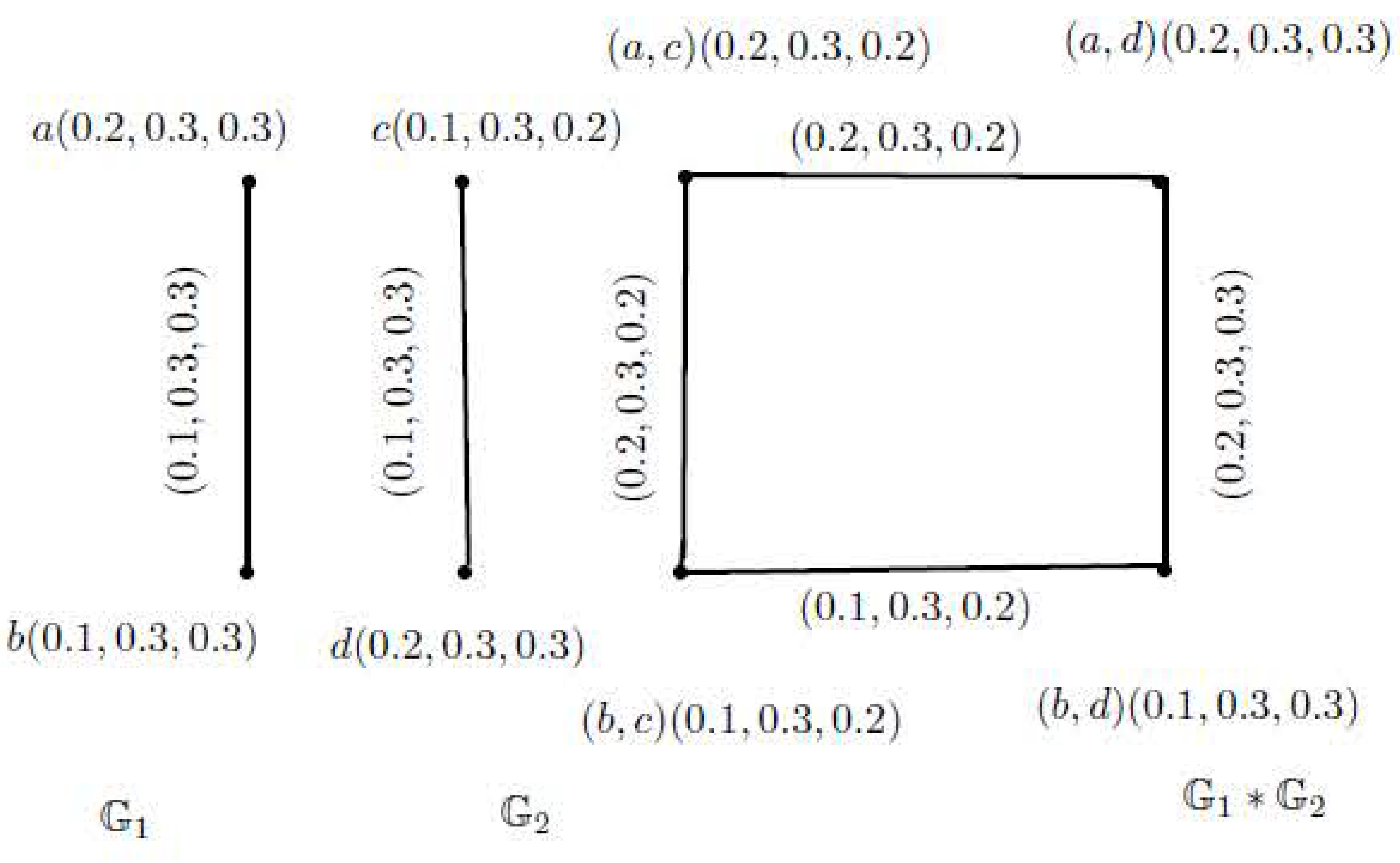
Definition 3.

A PFG $\mathbb{G}$ is said to be strong if

$$\begin{array}{c}\hfill {\chi }_W\left(uw\right)=\wedge \{{\chi }_U\left(u\right),{\chi }_U\left(w\right)\},\end{array}$$

$$\begin{array}{c}\hfill {\varphi }_W\left(uw\right)=\wedge \{{\varphi }_U\left(u\right),{\varphi }_U\left(w\right)\},\end{array}$$

$$\begin{array}{c}\hfill {\psi }_W\left(uw\right)=\vee \{{\psi }_U\left(u\right),{\psi }_U\left(w\right)\},\end{array}$$

∀ uw ∈ V.

Definition 4.

A PFG $\mathbb{G}$ is said to be complete if

$$\begin{array}{c}\hfill {\chi }_W\left(uw\right)=\wedge \{{\chi }_U\left(u\right),{\chi }_U\left(w\right)\},\end{array}$$

$$\begin{array}{c}\hfill {\varphi }_W\left(uw\right)=\wedge \{{\varphi }_U\left(u\right),{\varphi }_U\left(w\right)\},\end{array}$$

$$\begin{array}{c}\hfill {\psi }_W\left(uw\right)=\vee \{{\psi }_U\left(u\right),{\psi }_U\left(w\right)\},\end{array}$$

∀ u, w ∈ E.

Definition 5.

The MP ${\mathbb{G}}_1\ast {\mathbb{G}}_2=(U_1\ast U_2,W_1\ast W_2)$ of two PFGs ${\mathbb{G}}_1=(U_1,W_1)$ and ${\mathbb{G}}_2=(U_2,W_2)$ is defined as:

(i)

$$\begin{array}{c}\hfill ({\chi }_{U_1}\ast {\chi }_{U_2})(u_1,u_2)=\vee \{{\chi }_{U_1}\left(u_1\right),{\chi }_{U_2}\left(u_2\right)\},\end{array}$$

$$\begin{array}{c}\hfill ({\varphi }_{U_1}\ast {\varphi }_{U_2})(u_1,u_2)=\vee \{{\varphi }_{U_1}\left(u_1\right),{\varphi }_{U_2}\left(u_2\right)\},\end{array}$$

$$\begin{array}{c}\hfill ({\psi }_{U_1}\ast {\psi }_{U_2})(u_1,u_2)=\wedge \{{\psi }_{U_1}\left(u_1\right),{\psi }_{U_2}\left(u_2\right)\}\end{array}$$

$\forall (u_1,u_2)\in (V_1\times V_2)$.

(ii)

$$\begin{array}{c}\hfill ({\chi }_{U_1}\ast {\chi }_{U_2})\left((m,u_2)(m,w_2)\right)=\vee \{{\chi }_{U_1}\left(m\right),{\chi }_{W_2}\left(u_2{w}_2\right)\},\end{array}$$

$$\begin{array}{c}\hfill ({\varphi }_{U_1}\ast {\varphi }_{U_2})\left((m,u_2)(m,w_2)\right)=\vee \{{\varphi }_{U_1}\left(m\right),{\varphi }_{W_2}\left(u_2{w}_2\right)\},\end{array}$$

$$\begin{array}{c}\hfill ({\psi }_{U_1}\ast {\psi }_{U_2})\left((m,u_2)(m,w_2)\right)=\wedge \{{\psi }_{U_1}\left(m\right),{\psi }_{W_2}\left(u_2{w}_2\right)\}.\end{array}$$

$\forall m\in V_{1}and{u}_2{w}_2\in E_2$.

(iii)

$$\begin{array}{c}\hfill ({\chi }_{U_1}\ast {\chi }_{U_2})\left((u_1,z)(w_1,z)\right)=\vee \{{\chi }_{W_1}\left(u_1{w}_1\right),{\chi }_{U_2}\left(z\right)\},\end{array}$$

$$\begin{array}{c}\hfill ({\varphi }_{U_1}\ast {\varphi }_{U_2})\left((u_1,z)(w_1,z)\right)=\vee \{{\varphi }_{W_1}\left(u_1{w}_1\right),{\varphi }_{U_2}\left(z\right)\},\end{array}$$

$$\begin{array}{c}\hfill ({\psi }_{U_1}\ast {\psi }_{U_2})\left((u_1,z)(w_1,z)\right)=\wedge \{{\psi }_{W_1}\left(u_1{w}_1\right),{\psi }_{U_2}\left(z\right)\}.\end{array}$$

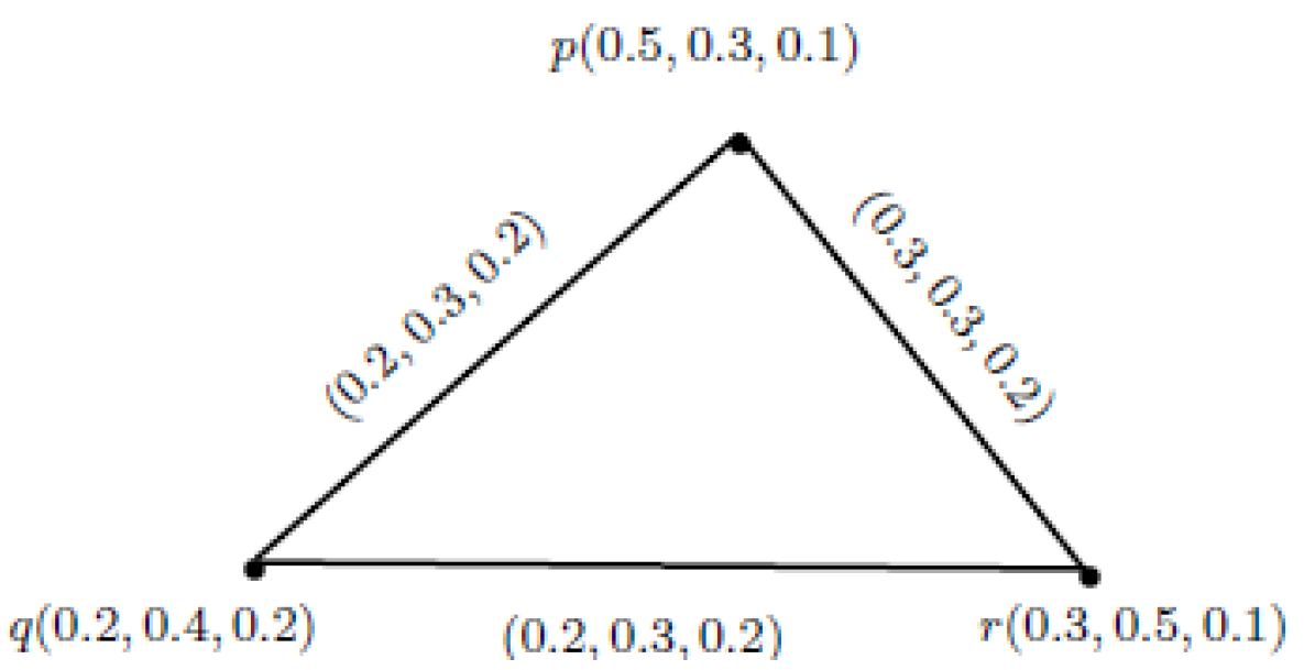
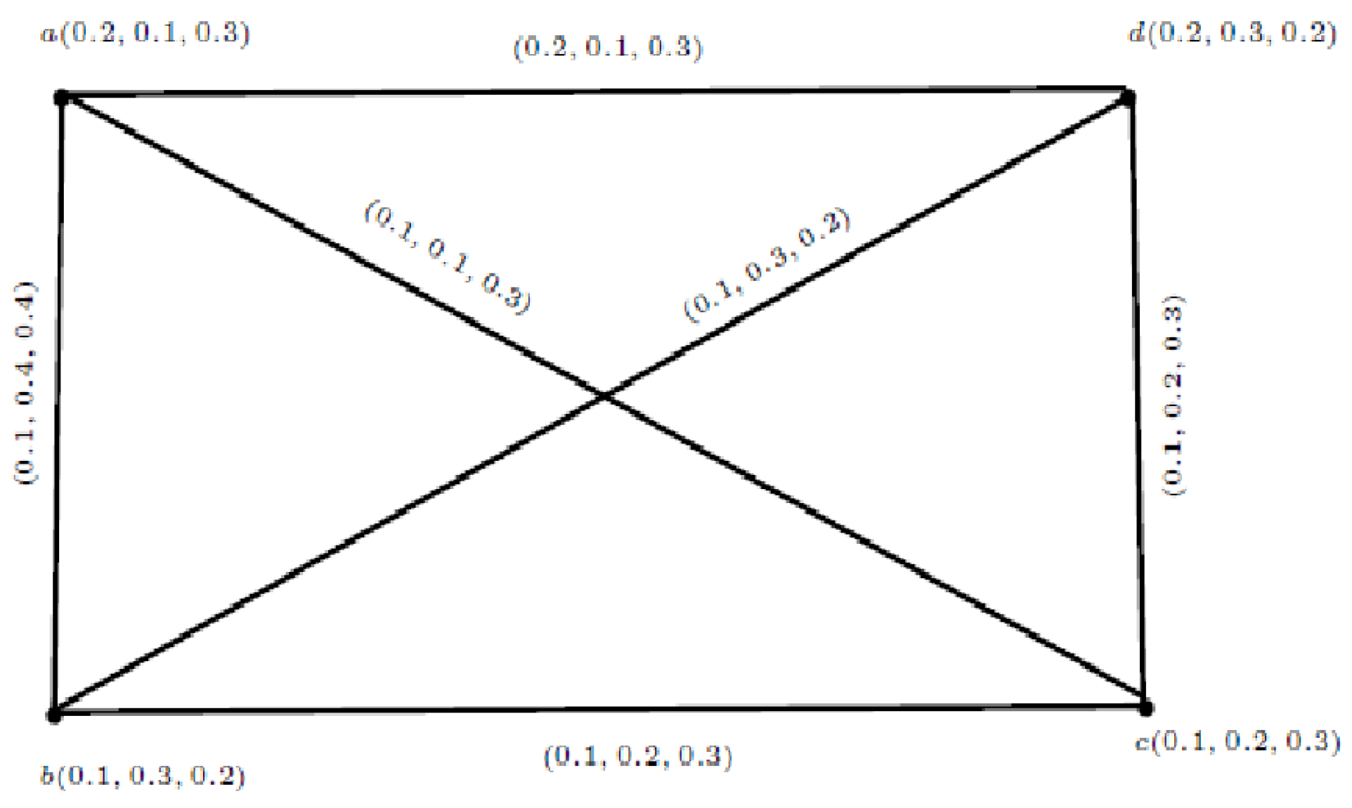
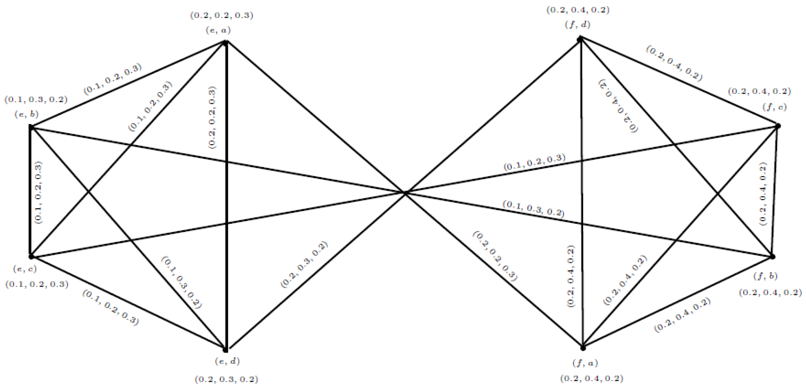
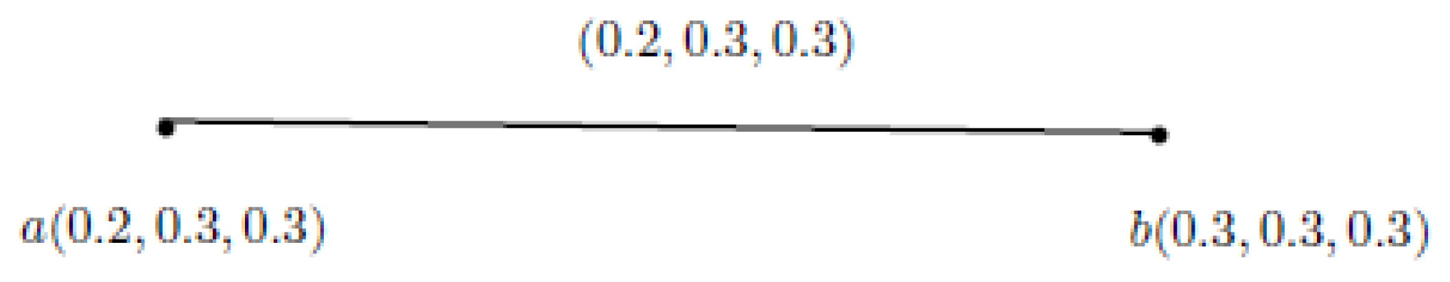
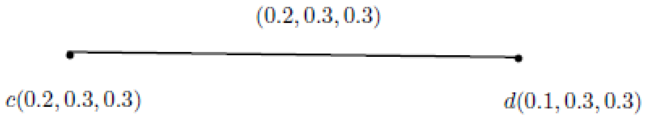
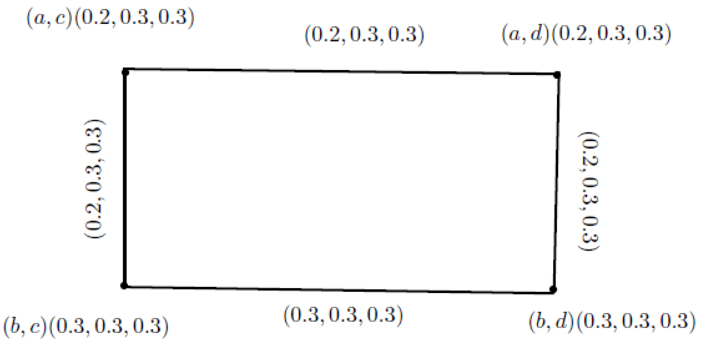
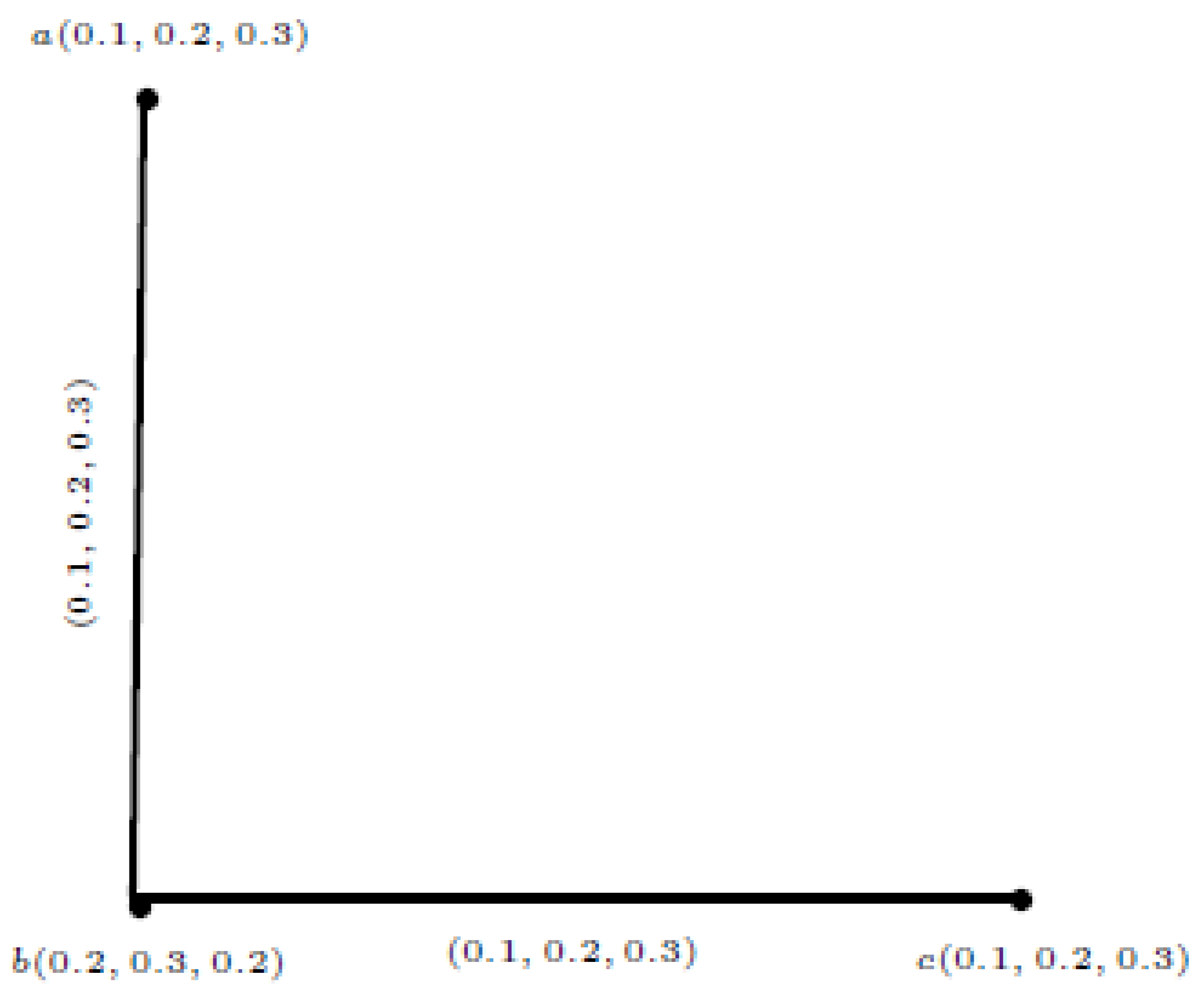
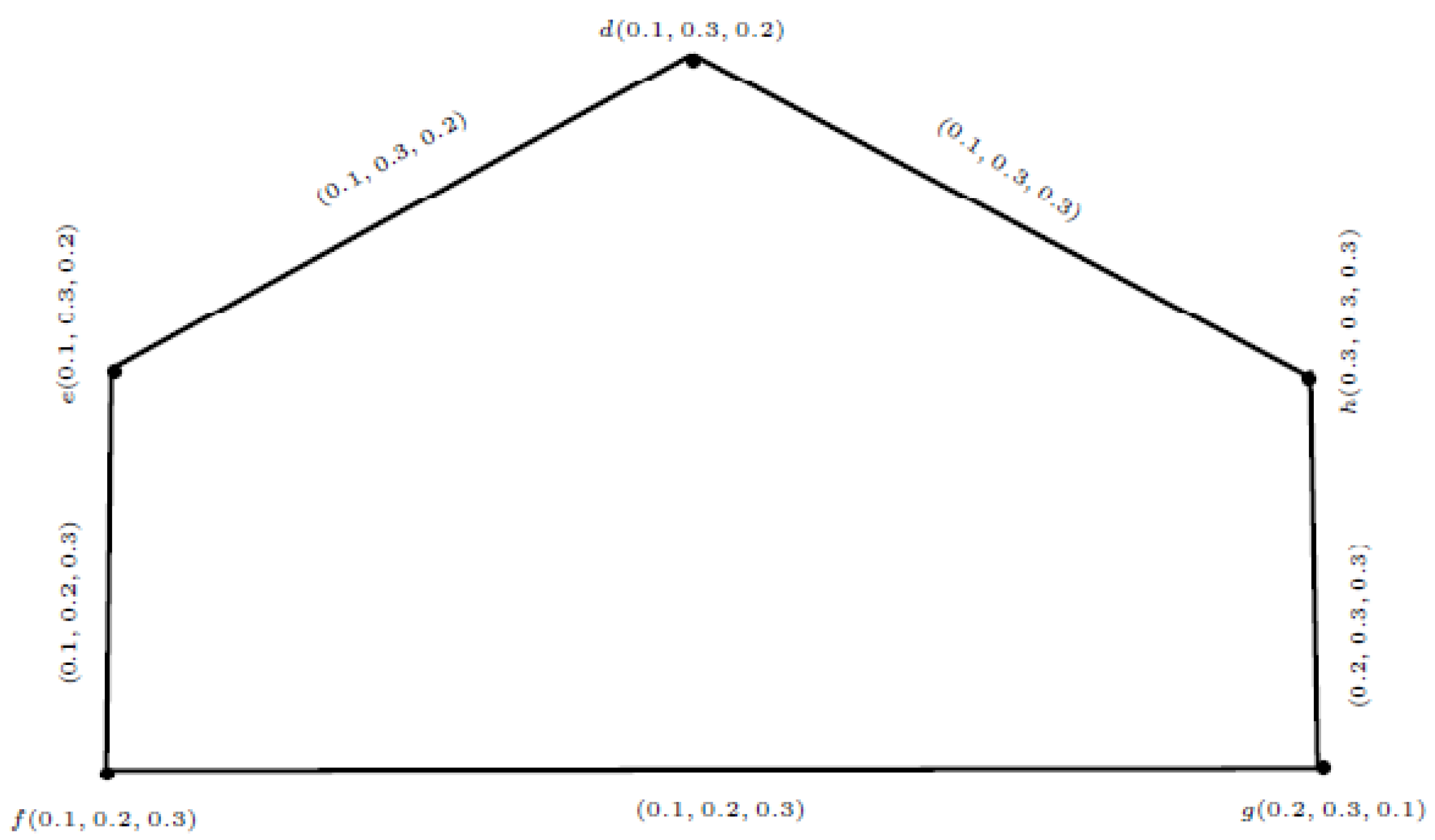
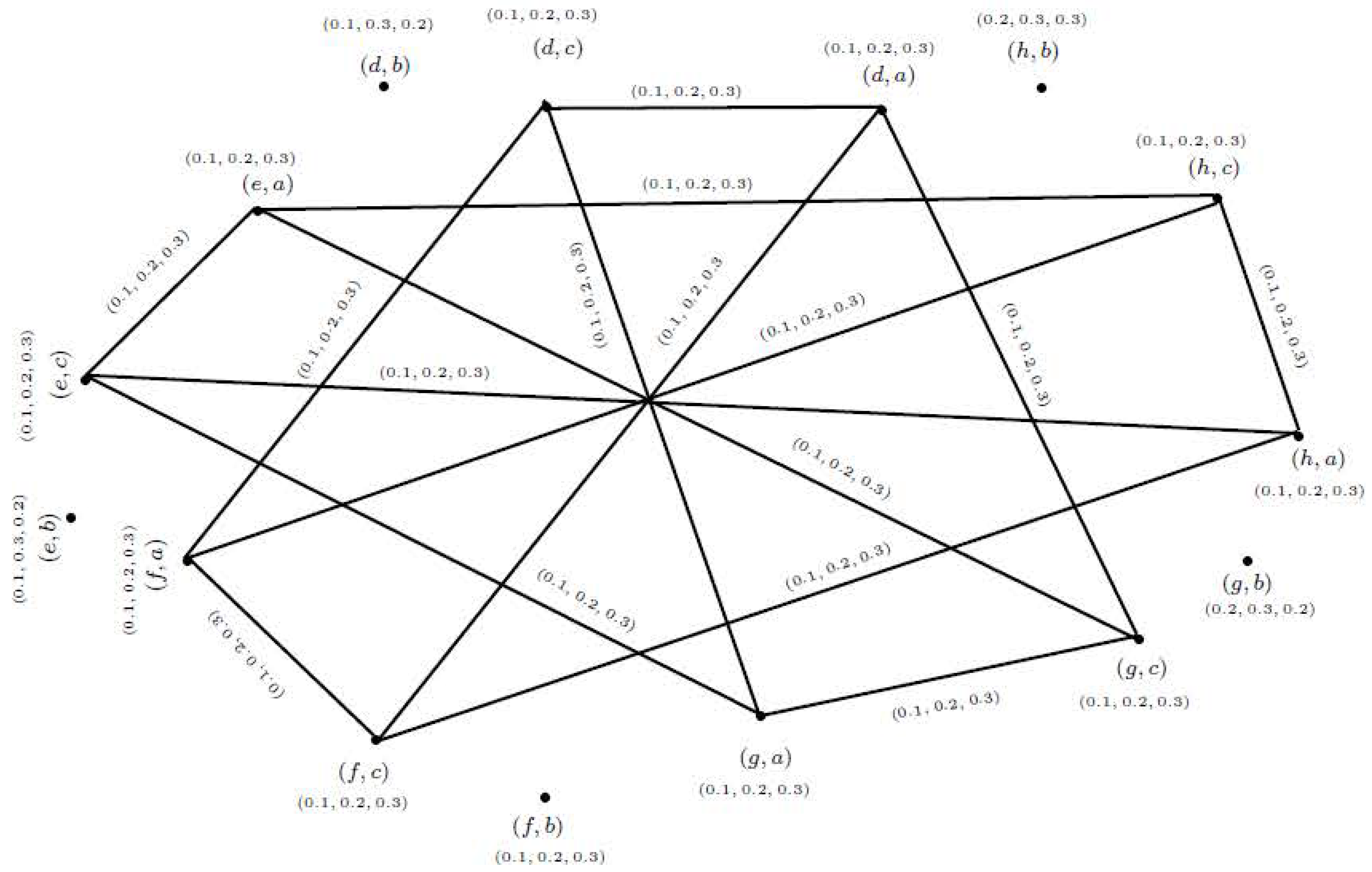
for all $z\in V_{2}and{u}_1{w}_1\in E_1$.

Example 2.

Suppose that ${\mathbb{G}}_1=(U_1,W_1)$ and ${\mathbb{G}}_2=(U_2,W_2)$ are two PFGs, which are shown in Figure 2 and Figure 3. Their MP ${\mathbb{G}}_1\ast {\mathbb{G}}_2$ is shown in Figure 4.

For vertex (e,a), we find the membership value (Mv), indeterminate value (IDv), and non-membership value (NMv) as follows:

$$\begin{array}{cc}\hfill ({\chi }_{U_1}\ast {\chi }_{U_2})(e,a)& =\vee \{{\chi }_{U_1}\left(e\right),{\chi }_{U_2}\left(a\right)\}\hfill \\ \hfill & =\vee \{0.1,0.2\}=0.2,\hfill \end{array}$$

$$\begin{array}{cc}\hfill ({\varphi }_{U_1}\ast {\varphi }_{U_2})(e,a)& =\vee \{{\varphi }_{U_1}\left(e\right),{\varphi }_{U_2}\left(a\right)\}\hfill \\ \hfill & =\vee \{0.2,0.1\}=0.2,\hfill \end{array}$$

$$\begin{array}{cc}\hfill ({\psi }_{U_1}\ast {\psi }_{U_2})(e,a)& =\wedge \{{\psi }_{U_1}\left(e\right),{\psi }_{U_2}\left(a\right)\}\hfill \\ \hfill & =\wedge \{0.3,0.3\}=0.3\hfill \end{array}$$

for $e\in V_1$ and $a\in V_2$.

For edge (e,a)(e,b), we find Mv, IDv, and NMv.

$$\begin{array}{cc}\hfill ({\chi }_{U_1}\ast {\chi }_{U_2})\left((e,a)(e,b)\right)& =\vee \{{\chi }_{U_1}\left(e\right),{\chi }_{W_2}\left(ab\right)\}\hfill \\ \hfill & =\vee \{0.1,0.1\}=0.1,\hfill \end{array}$$

$$\begin{array}{cc}\hfill ({\varphi }_{U_1}\ast {\varphi }_{U_2})\left((e,a)(e,b)\right)& =\vee \{{\varphi }_{U_1}\left(e\right),{\varphi }_{W_2}\left(ab\right)\}\hfill \\ \hfill & =\vee \{0.2,0.1\}=0.2,\hfill \end{array}$$

$$\begin{array}{cc}\hfill ({\psi }_{U_1}\ast {\psi }_{U_2})\left((e,a)(e,b)\right)& =\wedge \{{\psi }_{U_1}\left(e\right),{\psi }_{W_2}\left(ab\right)\}\hfill \\ \hfill & =\wedge \{0.3,0.3\}=0.3\hfill \end{array}$$

for $e\in V_1$ and $ab\in E_2$.

For edge $(e,a)(f,a)$:

$$\begin{array}{cc}\hfill ({\chi }_{U_1}\ast {\chi }_{U_2})\left((e,a)(f,a)\right)& =\vee \{{\chi }_{W_1}\left(ef\right),{\chi }_{U_2}\left(a\right)\}\hfill \\ \hfill & =\vee \{0.1,0.2\}=0.2,\hfill \end{array}$$

$$\begin{array}{cc}\hfill ({\varphi }_{U_1}\ast {\varphi }_{U_2})\left((e,a)(f,a)\right)& =\vee \{{\varphi }_{W_1}\left(ef\right),{\varphi }_{U_2}\left(a\right)\}\hfill \\ \hfill & =\vee \{0.2,0.1\}=0.2,\hfill \end{array}$$

$$\begin{array}{cc}\hfill ({\psi }_{U_1}\ast {\psi }_{U_2})\left((e,a)(f,a)\right)& =\wedge \{{\psi }_{W_1}\left(ef\right),{\psi }_{U_2}\left(a\right)\}\hfill \\ \hfill & =0.3\hfill \end{array}$$

for $a\in V_2$ and $ef\in E_1$.

Mv, IDv, and NMv can be similarly calculated for all other nodes and edges.

Proposition 1.

The MP of two PFGs ${\mathbb{G}}_1$ and ${\mathbb{G}}_2$ is a PFG.

Proof. 

Suppose that ${\mathbb{G}}_1=(U_1,W_1)$ and ${\mathbb{G}}_2=(U_2,W_2)$ are two PFGs on crisp graphs $G_1=(V_1,E_1)$ and $G_2=(V_2,E_2)$, respectively, and $\left((u_1,u_2)(w_1,w_2)\right)\in E_1\times E_2$.

By using Definition 5:

(i) If $u_1=w_1=m$,

$$\begin{array}{cc}\hfill ({\chi }_{W_1}\ast {\chi }_{W_2})\left((m,u_2)(m,w_2)\right)& =\vee \{{\chi }_{U_1}\left(m\right),{\chi }_{W_2}\left(u_2{w}_2\right)\}\hfill \\ \hfill & \le \vee \{{\chi }_{U_1}\left(m\right),\wedge \{{\chi }_{U_2}\left(u_2\right),{\chi }_{U_2}\left(w_2\right)\}\}\hfill \\ \hfill & =\wedge \{\vee \{{\chi }_{U_1}\left(m\right),{\chi }_{U_2}\left(u_2\right)\},\vee \{{\chi }_{U_1}\left(m\right),{\chi }_{U_2}\left(w_2\right)\}\}\hfill \\ \hfill & =\wedge \{({\chi }_{U_1}\ast {\chi }_{U_2})(m,u_2),({\chi }_{U_1}\ast {\chi }_{U_2})(m,w_2)\},\hfill \end{array}$$

$$\begin{array}{cc}\hfill ({\varphi }_{W_1}\ast {\varphi }_{W_2})\left((m,u_2)(m,w_2)\right)& =\vee \{{\varphi }_{U_1}\left(m\right),{\varphi }_{W_2}\left(u_2{w}_2\right)\}\hfill \\ \hfill & \le \vee \{{\varphi }_{U_1}\left(m\right),\wedge \{{\varphi }_{U_2}\left(u_2\right),{\varphi }_{U_2}\left(w_2\right)\}\}\hfill \\ \hfill & =\wedge \{\vee \{{\varphi }_{U_1}\left(m\right),{\varphi }_{U_2}\left(u_2\right)\},\vee \left\{{\varphi }_{U_1}\left(m\right),{\varphi }_{U_2}\left(w_2\right)\}\right\}\hfill \\ \hfill & =\wedge \{({\varphi }_{U_1}\ast {\varphi }_{U_2})(m,u_2),({\varphi }_{U_1}\ast {\varphi }_{U_2})(m,w_2)\},\hfill \end{array}$$

$$\begin{array}{cc}\hfill ({\psi }_{W_1}\ast {\psi }_{W_2})\left((m,u_2)(m,w_2)\right)& =\wedge \{{\psi }_{U_1}\left(m\right),{\psi }_{W_2}\left(u_2{w}_2\right)\}\hfill \\ \hfill & \ge \wedge \{{\psi }_{U_1}\left(m\right),\vee \{{\psi }_{U_2}\left(u_2\right),{\psi }_{U_2}\left(w_2\right)\}\}\hfill \\ \hfill & =\vee \{\wedge \{{\psi }_{U_1}\left(m\right),{\psi }_{U_2}\left(u_2\right)\},\wedge \left\{{\psi }_{U_1}\left(m\right),{\psi }_{U_2}\left(w_2\right)\}\right\}\hfill \\ \hfill & =\vee \{({\psi }_{U_1}\ast {\psi }_{U_2})(m,u_2),({\psi }_{U_1}\ast {\psi }_{U_2})(m,w_2)\}.\hfill \end{array}$$

(ii) If $u_2=w_2=z$,

$$\begin{array}{cc}\hfill ({\chi }_{W_1}\ast {\chi }_{W_2})\left((u_1,z)(w_1,z)\right)& =\vee \{{\chi }_{W_1}\left(u_1{w}_1\right),{\chi }_{U_2}\left(z\right)\}\hfill \\ \hfill & \le \vee \{\wedge \{{\chi }_{W_1}\left(u_1{w}_1\right),{\chi }_{U_2}\left(z\right)\}\hfill \\ \hfill & =\wedge \{\vee \{{\chi }_{W_1}\left(u_1\right),{\chi }_{U_2}\left(z\right)\},\vee \{{\chi }_{U_1}\left(w_1\right),{\chi }_{U_2}\left(z\right)\}\}\hfill \\ \hfill & =\wedge \{({\chi }_{U_1}\ast {\chi }_{U_2})(u_1,z),({\chi }_{U_1}\ast {\chi }_{U_2})(w_1,z)\},\hfill \end{array}$$

$$\begin{array}{cc}\hfill ({\varphi }_{W_1}\ast {\varphi }_{W_2})\left((u_1,z)(w_1,z)\right)& =\vee \{{\varphi }_{W_1}\left(u_1{w}_1\right),{\varphi }_{U_2}\left(z\right)\}\hfill \\ \hfill & \le \vee \{\wedge \{{\varphi }_{W_1}\left(u_1{w}_1\right),{\varphi }_{U_2}\left(z\right)\}\hfill \\ \hfill & =\wedge \{\vee \{{\varphi }_{U_1}\left(u_1\right),{\varphi }_{U_2}\left(z\right)\},\vee \{{\varphi }_{U_1}\left(w_1\right),{\varphi }_{U_2}\left(z\right)\}\}\hfill \\ \hfill & =\wedge \{({\varphi }_{U_1}\ast {\varphi }_{U_2})(u_1,z),({\varphi }_{U_1}\ast {\varphi }_{U_2})(w_1,z)\},\hfill \end{array}$$

$$\begin{array}{cc}\hfill ({\psi }_{W_1}\ast {\psi }_{W_2})\left((u_1,z)(w_1,z)\right)& =\wedge \{{\psi }_{W_1}\left(u_1{w}_1\right),{\psi }_{U_2}\left(z\right)\}\hfill \\ \hfill & \ge \wedge \{\vee \{{\psi }_{W_1}\left(u_1{w}_1\right),{\psi }_{U_2}\left(z\right)\}\hfill \\ \hfill & =\vee \{\wedge \{{\psi }_{U_1}\left(u_1\right),{\psi }_{U_2}\left(z\right)\},\wedge \{{\psi }_{U_1}\left(w_1\right),{\psi }_{U_2}\left(z\right)\}\}\hfill \\ \hfill & =\vee \{({\psi }_{U_1}\ast {\psi }_{U_2})(u_1,z),({\psi }_{U_1}\ast {\psi }_{U_2})(w_1,z)\}.\hfill \end{array}$$

We conclude that ${\mathbb{G}}_1\ast {\mathbb{G}}_2$ is a PFG. □

Theorem 1.

The MP of two strong PFGs ${\mathbb{G}}_1$ and ${\mathbb{G}}_2$ is a strong PFG.

Proof. 

Suppose that ${\mathbb{G}}_1=(U_1,W_1)$ and ${\mathbb{G}}_2=(U_2,W_2)$ are two strong PFGs on two crisp graphs and $\left((u_1,u_2)(w_1,w_2)\right)\in E_1\times E_2$.

By using Proposition 1, we obtain:

(i) If $u_1=w_1=m$,

$$\begin{array}{cc}\hfill ({\chi }_{W_1}\ast {\chi }_{W_2})\left((m,u_2)(m,w_2)\right)& =\vee \{{\chi }_{U_1}\left(m\right),{\chi }_{W_2}\left(u_2{w}_2\right)\}\hfill \\ \hfill & =\vee \{{\chi }_{U_1}\left(m\right),\wedge \{{\chi }_{U_2}\left(u_2\right),{\chi }_{U_2}\left(w_2\right)\}\}\hfill \\ \hfill & =\wedge \{\vee \{{\chi }_{U_1}\left(m\right),{\chi }_{U_2}\left(u_2\right)\},\vee \{{\chi }_{U_1}\left(m\right),{\chi }_{U_2}\left(w_2\right)\}\}\hfill \\ \hfill & =\wedge \{({\chi }_{U_1}\ast {\chi }_{U_2})(m,u_2),({\chi }_{U_1}\ast {\chi }_{U_2})(m,w_2)\},\hfill \end{array}$$

$$\begin{array}{cc}\hfill ({\varphi }_{W_1}\ast {\varphi }_{W_2})\left((m,u_2)(m,w_2)\right)& =\vee \{{\varphi }_{U_1}\left(m\right),{\varphi }_{W_2}\left(u_2{w}_2\right)\}\hfill \\ \hfill & =\vee \{{\varphi }_{U_1}\left(m\right),\wedge \{{\varphi }_{U_2}\left(u_2\right),{\varphi }_{U_2}\left(w_2\right)\}\}\hfill \\ \hfill & =\wedge \{\vee \{{\varphi }_{U_1}\left(m\right),{\varphi }_{U_2}\left(u_2\right)\},\vee \{{\varphi }_{U_1}\left(m\right),{\varphi }_{U_2}\left(w_2\right)\}\}\hfill \\ \hfill & =\wedge \{({\varphi }_{U_1}\ast {\varphi }_{U_2})(m,u_2),({\varphi }_{U_1}\ast {\varphi }_{U_2})(m,w_2)\},\hfill \end{array}$$

$$\begin{array}{cc}\hfill ({\psi }_{W_1}\ast {\psi }_{W_2})\left((m,u_2)(m,w_2)\right)& =\wedge \{{\psi }_{U_1}\left(m\right),{\psi }_{W_2}\left(u_2{w}_2\right)\}\hfill \\ \hfill & =\wedge \{{\psi }_{U_1}\left(m\right),\vee \{{\psi }_{U_2}\left(u_2\right),{\psi }_{U_2}\left(w_2\right)\}\}\hfill \\ \hfill & =\vee \{\wedge \{{\psi }_{U_1}\left(m\right),{\psi }_{U_2}\left(u_2\right)\},\wedge \{{\psi }_{U_1}\left(m\right),{\psi }_{U_2}\left(w_2\right)\}\}\hfill \\ \hfill & =\vee \{({\psi }_{U_1}\ast {\psi }_{U_2})(m,u_2),({\psi }_{U_1}\ast {\psi }_{U_2})(m,w_2)\}.\hfill \end{array}$$

(ii) If $u_2=w_2=z$,

$$\begin{array}{cc}\hfill ({\chi }_{W_1}\ast {\chi }_{W_2})\left((u_1,z)(w_1,z)\right)& =\vee \{{\chi }_{W_1}\left(u_1{w}_1\right),{\chi }_{U_2}\left(z\right)\}\hfill \\ \hfill & =\vee \{\wedge \{{\chi }_{W_1}\left(u_1{w}_1\right),{\chi }_{U_2}\left(z\right)\}\hfill \\ \hfill & =\wedge \{\vee \{{\chi }_{W_1}\left(u_1\right),{\chi }_{U_2}\left(z\right)\},\vee \{{\chi }_{U_1}\left(w_1\right),{\chi }_{U_2}\left(z\right)\}\}\hfill \\ \hfill & =\wedge \{({\chi }_{U_1}\ast {\chi }_{U_2})(u_1,z),({\chi }_{U_1}\ast {\chi }_{U_2})(w_1,z)\},\hfill \end{array}$$

$$\begin{array}{cc}\hfill ({\varphi }_{W_1}\ast {\varphi }_{W_2})\left((u_1,z)(w_1,z)\right)& =\vee \{{\varphi }_{W_1}\left(u_1{w}_1\right),{\varphi }_{U_2}\left(z\right)\}\hfill \\ \hfill & =\vee \{\wedge \{{\varphi }_{W_1}\left(u_1{w}_1\right),{\varphi }_{U_2}\left(z\right)\}\hfill \\ \hfill & =\wedge \{\vee \{{\varphi }_{U_1}\left(u_1\right),{\varphi }_{U_2}\left(z\right)\},\vee \{{\varphi }_{U_1}\left(w_1\right),{\varphi }_{U_2}\left(z\right)\}\}\hfill \\ \hfill & =\wedge \{({\varphi }_{U_1}\ast {\varphi }_{U_2})(u_1,z),({\varphi }_{U_1}\ast {\varphi }_{U_2})(w_1,z)\},\hfill \end{array}$$

$$\begin{array}{cc}\hfill ({\psi }_{W_1}\ast {\psi }_{W_2})\left((u_1,z)(w_1,z)\right)& =\wedge \{{\psi }_{W_1}\left(u_1{w}_1\right),{\psi }_{U_2}\left(z\right)\}\hfill \\ \hfill & =\wedge \{\vee \{{\psi }_{W_1}\left(u_1{w}_1\right),{\psi }_{U_2}\left(z\right)\}\hfill \\ \hfill & =\vee \{\wedge \{{\psi }_{U_1}\left(u_1\right),{\psi }_{U_2}\left(z\right)\},\wedge \{{\psi }_{U_1}\left(w_1\right),{\psi }_{U_2}\left(z\right)\}\}\hfill \\ \hfill & =\vee \{({\psi }_{U_1}\ast {\psi }_{U_2})(u_1,z),({\psi }_{U_1}\ast {\psi }_{U_2})(w_1,z)\}.\hfill \end{array}$$

Hence, ${\mathbb{G}}_1\ast {\mathbb{G}}_2$ is a strong PFG. □

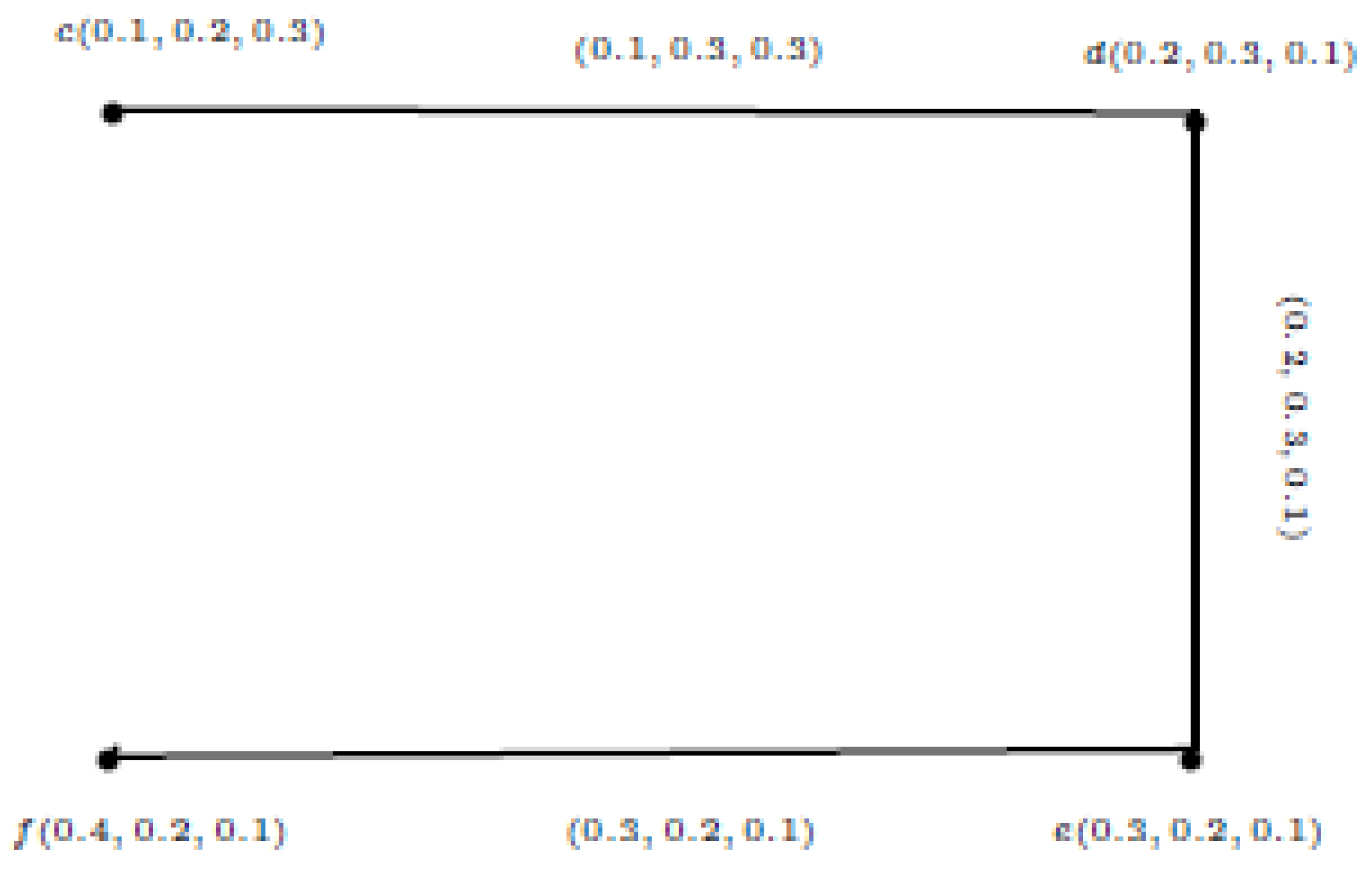
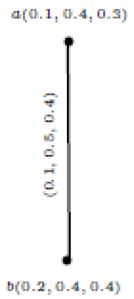
Example 3.

Suppose that ${\mathbb{G}}_1$ and ${\mathbb{G}}_2$ are two strong PFGs, as shown in Figure 5.

Hence, $G_1\ast G_2$ is also a strong PFG.

Remark 1.

If the MP of two PFGs ${\mathbb{G}}_1=(U_1,W_1)$ and ${\mathbb{G}}_2=(U_2,W_2)$ is strong, then ${\mathbb{G}}_1=(U_1,W_1)$ and ${\mathbb{G}}_2=(U_2,W_2)$ are not required to be strong, in general.

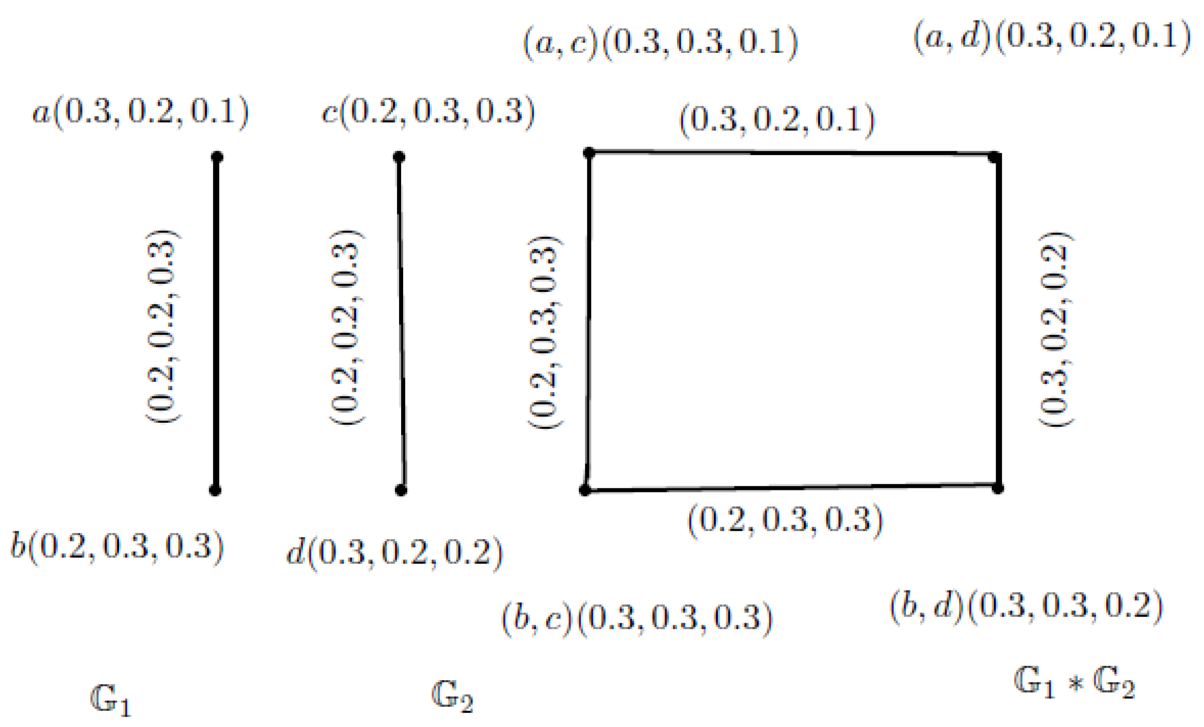
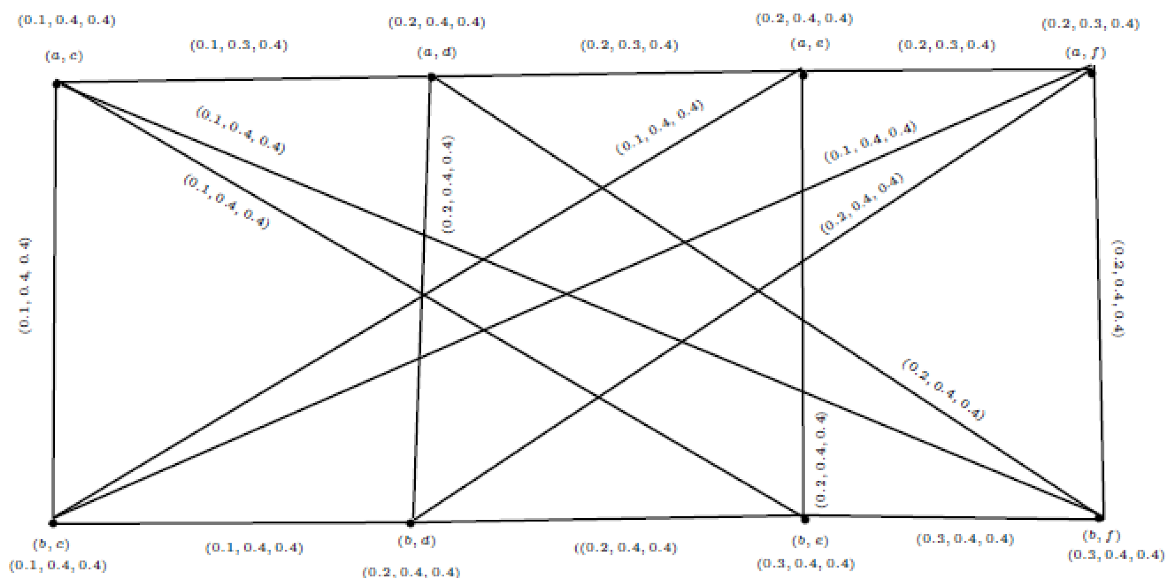
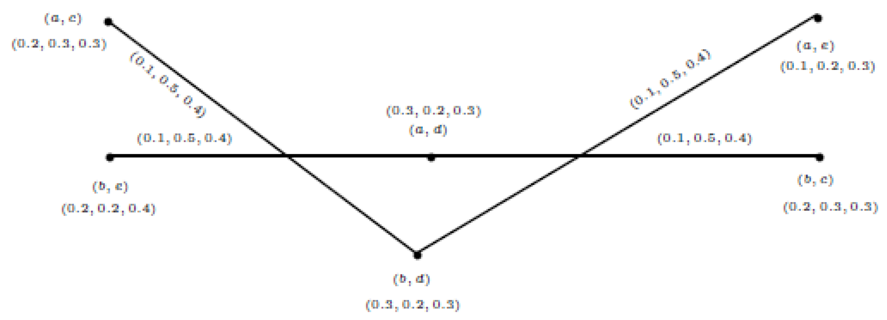
Example 4.

Suppose that ${\mathbb{G}}_1$ and ${\mathbb{G}}_2$ are two PFGs, as in Figure 6 and Figure 7. We can see the MP of the two PFGs ${\mathbb{G}}_1$ and ${\mathbb{G}}_2$, that is, ${\mathbb{G}}_1\ast {\mathbb{G}}_2$, in Figure 8.

Then, ${\mathbb{G}}_1$ and ${\mathbb{G}}_1\ast {\mathbb{G}}_2$ are strong PFGs, but ${\mathbb{G}}_2$ is not strong.

Since ${\chi }_{W_2}(u_2,w_2)$=0.2, on other hand, $\wedge \{{\chi }_{U_2}\left(u_2\right),{\chi }_{U_2}\left(w_2\right\}$=$\wedge \{0.2,0.1\}$=0.1.

Hence, ${\chi }_{W_2}(u_2,w_2)\ne \wedge \{{\chi }_{U_2}\left(u_2\right),{\chi }_{U_2}\left(w_2\right\}$.

Remark 2.

The MP of two complete PFGs may or may not be a complete PFG.

Definition 6.

Suppose that ${\mathbb{G}}_1=(U_1,W_1)$ and ${\mathbb{G}}_2=(U_2,W_2)$ are two PFGs. $\forall (u_1,u_2)\in V_1\times V_2$,

$$\begin{array}{cc}\hfill {\left(d_{\chi }\right)}_{{\mathbb{G}}_1\ast {\mathbb{G}}_2}(u_1,u_2)& =\sum _{(u_1,u_2)(w_1,w_2)\in E_1\times E_2.}({\chi }_{W_1}\ast {\chi }_{W_2})\left((u_1,u_2)(w_1,w_2)\right)\hfill \\ \hfill & =\sum _{u_1=w_1,u_2{w}_2\in E_2}\vee \{{\chi }_{U_1}\left(u_1\right),{\chi }_{W_2}\left(u_2{w}_2\right)\}\hfill \\ \hfill & +\sum _{u_1{w}_1\in E_1,u_2=w_2}\vee \{{\chi }_{W_1}\left(u_1{w}_1\right),{\chi }_{U_2}\left(u_2\right)\},\hfill \end{array}$$

$$\begin{array}{cc}\hfill {\left(d_{\varphi }\right)}_{{\mathbb{G}}_1\ast {\mathbb{G}}_2}(u_1,u_2)& =\sum _{(u_1,u_2)(w_1,w_2)\in E_1\times E_2.}({\varphi }_{W_1}\ast {\varphi }_{W_2})\left((u_1,u_2)(w_1,w_2)\right)\hfill \\ \hfill & =\sum _{u_1=w_1,u_2{w}_2\in E_2}\vee \{{\varphi }_{U_1}\left(u_1\right),{\varphi }_{W_2}\left(u_2{w}_2\right)\}\hfill \\ \hfill & +\sum _{u_1{w}_1\in E_1,u_2=w_2}\vee \{{\varphi }_{W_1}\left(u_1{w}_1\right),{\varphi }_{U_2}\left(u_2\right)\},\hfill \end{array}$$

$$\begin{array}{cc}\hfill {\left(d_{\psi }\right)}_{{\mathbb{G}}_1\ast {\mathbb{G}}_2}(u_1,u_2)& =\sum _{(u_1,u_2)(w_1,w_2)\in E_1\times E_2.}({\psi }_{W_1}\ast {\psi }_{W_2})\left((u_1,u_2)(w_1,w_2)\right)\hfill \\ \hfill & =\sum _{u_1=w_1,u_2{w}_2\in E_2}\wedge \{{\psi }_{U_1}\left(u_1\right),{\psi }_{W_2}\left(u_2{w}_2\right)\}\hfill \\ \hfill & +\sum _{u_1{w}_1\in E_1,u_2=w_2}\wedge \{{\psi }_{W_1}\left(u_1{w}_1\right),{\psi }_{U_2}\left(u_2\right)\}.\hfill \end{array}$$

Theorem 2.

Suppose that ${\mathbb{G}}_1=(U_1,W_1)$ and ${\mathbb{G}}_2=(U_2,W_2)$ are two PFGs. If ${\chi }_{U_1}\ge {\chi }_{W_2},{\varphi }_{U_1}\ge {\varphi }_{W_2},{\psi }_{U_1}\le {\psi }_{W_2}$ and ${\chi }_{U_2}\ge {\chi }_{W_1},{\varphi }_{U_2}\ge {\varphi }_{W_1},{\psi }_{U_2}\le {\psi }_{W_1}$, then for every $\forall (u_1,u_2)\in V_1\times V_2$,

$$\begin{array}{c}\hfill {\left(d_{\chi }\right)}_{{\mathbb{G}}_1\ast {\mathbb{G}}_2}(u_1,u_2)={\left(d\right)}_{G_2}\left(u_2\right){\chi }_{U_1}\left(u_1\right)+{\left(d\right)}_{G_1}\left(u_1\right){\chi }_{U_2}\left(u_2\right),\\ \hfill {\left(d_{\varphi }\right)}_{{\mathbb{G}}_1\ast {\mathbb{G}}_2}(u_1,u_2)={\left(d\right)}_{G_2}\left(u_2\right){\varphi }_{U_1}\left(u_1\right)+{\left(d\right)}_{G_1}\left(u_1\right){\varphi }_{U_2}\left(u_2\right),\\ \hfill {\left(d_{\psi }\right)}_{{\mathbb{G}}_1\ast {\mathbb{G}}_2}(u_1,u_2)={\left(d\right)}_{G_2}\left(u_2\right){\psi }_{U_1}\left(u_1\right)+{\left(d\right)}_{G_1}\left(u_1\right){\psi }_{U_2}\left(u_2\right).\end{array}$$

Proof. 

$$\begin{array}{cc}\hfill {\left(d_{\chi }\right)}_{{\mathbb{G}}_1\ast {\mathbb{G}}_2}(u_1,u_2)& =\sum _{(u_1,u_2)(w_1,w_2)\in E_1\times E_2.}({\chi }_{W_1}\ast {\chi }_{W_2})\left((u_1,u_2)(w_1,w_2)\right)\hfill \\ \hfill & =\sum _{u_1=w_1,u_2{w}_2\in E_2}\vee \{{\chi }_{U_1}\left(u_1\right),{\chi }_{W_2}\left(u_2{w}_2\right)\}\hfill \\ \hfill & +\sum _{u_1{w}_1\in E_1,u_2=w_2}\vee \{{\chi }_{W_1}\left(u_1{w}_1\right),{\chi }_{U_2}\left(u_2\right)\}\hfill \\ \hfill & =\sum _{u_2{w}_2\in E_2,u_1=w_1}{\chi }_{W_2}\left(u_2{w}_2\right)+\sum _{u_1{w}_1\in E_1,u_2=w_2}{\chi }_{W_1}\left(u_1{w}_1\right)\hfill \\ \hfill & ={\left(d\right)}_{G_2}\left(u_2\right){\chi }_{U_1}\left(u_1\right)+{\left(d\right)}_{G_1}\left(u_1\right){\chi }_{U_2}\left(u_2\right),\hfill \end{array}$$

$$\begin{array}{cc}\hfill {\left(d_{\varphi }\right)}_{{\mathbb{G}}_1\ast {\mathbb{G}}_2}(u_1,u_2)& =\sum _{(u_1,u_2)(w_1,w_2)\in E_1\times E_2.}({\varphi }_{W_1}\ast {\varphi }_{W_2})\left((u_1,u_2)(w_1,w_2)\right)\hfill \\ \hfill & =\sum _{u_1=w_1,u_2{w}_2\in E_2}\vee \{{\varphi }_{U_1}\left(u_1\right),{\varphi }_{W_2}\left(u_2{w}_2\right)\}\hfill \\ \hfill & +\sum _{u_1{w}_1\in E_1,u_2=w_2}\vee \{{\varphi }_{W_1}\left(u_1{w}_1\right),{\varphi }_{U_2}\left(u_2\right)\}\hfill \\ \hfill & =\sum _{u_2{w}_2\in E_2,u_1=w_1}{\varphi }_{W_2}\left(u_2{w}_2\right)+\sum _{u_1{w}_1\in E_1,u_2=w_2}{\varphi }_{W_1}\left(u_1{w}_1\right)\hfill \\ \hfill & ={\left(d\right)}_{G_2}\left(u_2\right){\varphi }_{U_1}\left(u_1\right)+{\left(d\right)}_{G_1}\left(u_1\right){\varphi }_{U_2}\left(u_2\right),\hfill \end{array}$$

$$\begin{array}{cc}\hfill {\left(d_{\psi }\right)}_{{\mathbb{G}}_1\ast {\mathbb{G}}_2}(u_1,u_2)& =\sum _{(u_1,u_2)(w_1,w_2)\in E_1\times E_2.}({\psi }_{W_1}\ast {\psi }_{W_2})\left((u_1,u_2)(w_1,w_2)\right)\hfill \\ \hfill & =\sum _{u_1=w_1,u_2{w}_2\in E_2}\wedge \{{\psi }_{U_1}\left(u_1\right),{\psi }_{W_2}\left(u_2{w}_2\right)\}\hfill \\ \hfill & +\sum _{u_1{w}_1\in E_1,u_2=w_2}\wedge \{{\psi }_{W_1}\left(u_1{w}_1\right),{\psi }_{U_2}\left(u_2\right)\}\hfill \\ \hfill & =\sum _{u_2{w}_2\in E_2,u_1=w_1}{\psi }_{W_2}\left(u_2{w}_2\right)+\sum _{u_1{w}_1\in E_1,u_2=w_2}{\psi }_{W_1}\left(u_1{w}_1\right)\hfill \\ \hfill & ={\left(d\right)}_{G_2}\left(u_2\right){\psi }_{U_1}\left(u_1\right)+{\left(d\right)}_{G_1}\left(u_1\right){\psi }_{U_2}\left(u_2\right).\hfill \end{array}$$

□

Example 5.

Taking PFGs ${\mathbb{G}}_1$, ${\mathbb{G}}_2$, and ${\mathbb{G}}_1\ast {\mathbb{G}}_2$, as in Figure 9, since ${\chi }_{U_1}\ge {\chi }_{W_2}$, ${\varphi }_{U_1}\ge {\varphi }_{W_2}$, ${\psi }_{U_1}\le {\psi }_{W_2}$, ${\chi }_{U_2}\ge {\chi }_{W_1}$${\varphi }_{U_2}\ge {\varphi }_{W_1}$, and ${\psi }_{U_2}\le {\psi }_{W_1}$, by Theorem 2, we have:

$$\begin{array}{ccc}& & {\left(d_{\chi }\right)}_{G_1\ast G_2}(a,d)={\left(d\right)}_{G_2}\left(d\right){\chi }_{U_1}\left(a\right)+{\left(d\right)}_{G_1}\left(a\right){\chi }_{U_2}\left(d\right)=1·\left(0.3\right)+1·\left(0.3\right)=0.6,\hfill \\ & & {\left(d_{\varphi }\right)}_{G_1\ast G_2}(a,d)={\left(d\right)}_{G_2}\left(d\right){\varphi }_{U_1}\left(a\right)+{\left(d\right)}_{G_1}\left(a\right){\varphi }_{U_2}\left(d\right)=1·\left(0.2\right)+1·\left(0.2\right)=0.4,\hfill \\ & & {\left(d_{\psi }\right)}_{G_1\ast G_2}(a,d)=0.3.\hfill \end{array}$$

From direct calculations:

$$\begin{array}{ccc}& & {\left(d_{\chi }\right)}_{G_1\ast G_2}(b,d)=0.2+0.3=0.5,\hfill \\ & & {\left(d_{\varphi }\right)}_{G_1\ast G_2}(b,d)=0.3+0.2=0.5,\hfill \\ & & {\left(d_{\psi }\right)}_{G_1\ast G_2}(b,d)=0.3+0.2=0.5,\hfill \\ & & {\left(d_{\chi }\right)}_{G_1\ast G_2}(a,c)=0.5,\hfill \\ & & {\left(d_{\varphi }\right)}_{G_1\ast G_2}(a,c)=0.5,\hfill \\ & & {\left(d_{\psi }\right)}_{G_1\ast G_2}(a,c)=0.4,\hfill \\ & & {\left(d_{\chi }\right)}_{G_1\ast G_2}(a,d)=0.6,\hfill \\ & & {\left(d_{\varphi }\right)}_{G_1\ast G_2}(a,d)=0.4,\hfill \\ & & {\left(d_{\psi }\right)}_{G_1\ast G_2}(a,d)=0.3,\hfill \\ & & {\left(d_{\chi }\right)}_{G_1\ast G_2}(b,c)=0.4,\hfill \\ & & {\left(d_{\varphi }\right)}_{G_1\ast G_2}(b,c)=0.6,\hfill \\ & & {\left(d_{\psi }\right)}_{G_1\ast G_2}(b,c)=0.6.\hfill \end{array}$$

We conclude from the above calculations that “the degrees of nodes determined by using the formula of the above theorem and by the direct method are equal”.

Definition 7.

Let ${\mathbb{G}}_1=(U_1,W_1)$ and ${\mathbb{G}}_2=(U_2,W_2)$ be two PFGs. $\forall (u_1,u_2)\in V_1\times V_2$,

$$\begin{array}{cc}\hfill {\left(t{d}_{\chi }\right)}_{{\mathbb{G}}_1\ast {\mathbb{G}}_2}(u_1,u_2)& =\sum _{(u_1,u_2)(w_1,w_2)\in E_1\times E_2.}({\chi }_{W_1}\ast {\chi }_{W_2})\left((u_1,u_2)(w_1,w_2)\right)+({\chi }_{U_1}\ast {\chi }_{U_2}(u_1,u_2))\hfill \\ \hfill & =\sum _{u_1=w_1,u_2{w}_2\in E_2}\vee \{{\chi }_{U_1}\left(u_1\right),{\chi }_{W_2}\left(u_2{w}_2\right)\}\hfill \\ \hfill & +\sum _{u_1{w}_1\in E_1,u_2=w_2}\vee \{{\chi }_{W_1}\left(u_1{w}_1\right),{\chi }_{U_2}\left(u_2\right)\}\hfill \\ \hfill & +\vee \{{\chi }_{U_1}\left(u_1\right),{\chi }_{U_2}\left(u_2\right)\},\hfill \end{array}$$

$$\begin{array}{cc}\hfill {\left(t{d}_{\varphi }\right)}_{{\mathbb{G}}_1\ast {\mathbb{G}}_2}(u_1,u_2)& =\sum _{(u_1,u_2)(w_1,w_2)\in E_1\times E_2.}({\varphi }_{W_1}\ast {\varphi }_{W_2})\left((u_1,u_2)(w_1,w_2)\right)+({\varphi }_{U_1}\ast {\varphi }_{U_2}(u_1,u_2))\hfill \\ \hfill & =\sum _{u_1=w_1,u_2{w}_2\in E_2}\vee \{{\varphi }_{U_1}\left(u_1\right),{\varphi }_{W_2}\left(u_2{w}_2\right)\}\hfill \\ \hfill & +\sum _{u_1{w}_1\in E_1,u_2=w_2}\vee \{{\varphi }_{W_1}\left(u_1{w}_1\right),{\varphi }_{U_2}\left(u_2\right)\}\hfill \\ \hfill & +\vee \{{\varphi }_{U_1}\left(u_1\right),{\varphi }_{U_2}\left(u_2\right)\},\hfill \end{array}$$

$$\begin{array}{cc}\hfill {\left(t{d}_{\psi }\right)}_{{\mathbb{G}}_1\ast {\mathbb{G}}_2}(u_1,u_2)& =\sum _{(u_1,u_2)(w_1,w_2)\in E_1\times E_2.}({\psi }_{W_1}\ast {\psi }_{W_2})\left((u_1,u_2)(w_1,w_2)\right)+({\psi }_{U_1}\ast {\psi }_{U_2}(u_1,u_2))\hfill \\ \hfill & =\sum _{u_1=w_1,u_2{w}_2\in E_2}\wedge \{{\psi }_{U_1}\left(u_1\right),{\psi }_{W_2}\left(u_2{w}_2\right)\}\hfill \\ \hfill & +\sum _{u_1{w}_1\in E_1,u_2=w_2}\wedge \{{\psi }_{W_1}(u_1{w}_1,{\psi }_{U_2}\left(u_2\right)\}\hfill \\ \hfill & +\wedge \{{\psi }_{U_1}\left(u_1\right),{\psi }_{U_2}\left(u_2\right)\}.\hfill \end{array}$$

Theorem 3.

Suppose that ${\mathbb{G}}_1=(U_1,W_1)$ and ${\mathbb{G}}_2=(U_2,W_2)$ are two PFGs. If ${\chi }_{U_1}\ge {\chi }_{W_2},{\varphi }_{U_1}\ge {\varphi }_{W_2},{\psi }_{U_1}\le {\psi }_{W_2}$ and ${\chi }_{U_2}\ge {\chi }_{W_1},{\varphi }_{U_2}\ge {\varphi }_{W_1},{\psi }_{U_2}\le {\psi }_{W_1}$, then for every $\forall (u_1,u_2)\in V_1\times V_2$,

$$\begin{array}{c}\hfill {\left(t{d}_{\chi }\right)}_{{\mathbb{G}}_1\ast {\mathbb{G}}_2}(u_1,u_2)={\left(d\right)}_{G_2}\left(u_2\right){\chi }_{U_1}\left(u_1\right)+{\left(d\right)}_{G_1}\left(u_1\right){\chi }_{U_2}\left(u_2\right)+\vee \{{\chi }_{U_1}\left(u_1\right),{\chi }_{U_2}\left(u_2\right)\},\\ \hfill {\left(t{d}_{\varphi }\right)}_{{\mathbb{G}}_1\ast {\mathbb{G}}_2}(u_1,u_2)={\left(d\right)}_{G_2}\left(u_2\right){\varphi }_{U_1}\left(u_1\right)+{\left(d\right)}_{G_1}\left(u_1\right){\varphi }_{U_2}\left(u_2\right)+\vee \{{\varphi }_{U_1}\left(u_1\right),{\varphi }_{U_2}\left(u_2\right)\},\\ \hfill {\left(t{d}_{\psi }\right)}_{{\mathbb{G}}_1\ast {\mathbb{G}}_2}(u_1,u_2)={\left(d\right)}_{G_2}\left(u_2\right){\psi }_{U_1}\left(u_1\right)+{\left(d\right)}_{G_1}\left(u_1\right){\psi }_{U_2}\left(u_2\right)+\wedge \{{\psi }_{U_1}\left(u_1\right),{\psi }_{U_2}\left(u_2\right)\}.\end{array}$$

Proof. 

$$\begin{array}{cc}\hfill {\left(t{d}_{\chi }\right)}_{{\mathbb{G}}_1\ast {\mathbb{G}}_2}(u_1,u_2)& =\sum _{(u_1,u_2)(w_1,w_2)\in E_1\times E_2.}({\chi }_{W_1}\ast {\chi }_{W_2})\left((u_1,u_2)(w_1,w_2)\right)+({\chi }_{U_1}\ast {\chi }_{U_2})(u_1,u_2)\hfill \\ \hfill & =\sum _{u_1=w_1,u_2{w}_2\in E_2}\vee \{{\chi }_{U_1}\left(u_1\right),{\chi }_{W_2}\left(u_2{w}_2\right)\}\hfill \\ \hfill & +\sum _{u_1{w}_1\in E_1,u_2=w_2}\vee \{{\chi }_{W_1}\left(u_1{w}_1\right),{\chi }_{U_2}\left(u_2\right)\}\hfill \\ \hfill & +\vee \{{\chi }_{U_1}\left(u_1\right),{\chi }_{U_2}\left(u_2\right)\}\hfill \\ \hfill & =\sum _{u_2{w}_2\in E_2,u_1=w_1}{\chi }_{W_2}\left(u_2{w}_2\right)+\sum _{u_1{w}_1\in E_1,u_2=w_2}{\chi }_{W_1}\left(u_1{w}_1\right)\hfill \\ \hfill & +max\{{\chi }_{U_1}\left(u_1\right),{\chi }_{U_2}\left(u_2\right)\}\hfill \\ \hfill & ={\left(d\right)}_{G_2}\left(u_2\right){\chi }_{U_1}\left(u_1\right)+{\left(d\right)}_{G_1}\left(u_1\right){\chi }_{U_2}\left(u_2\right)+max\{{\chi }_{U_1}\left(u_1\right),{\chi }_{U_2}\left(u_2\right)\}\hfill \end{array}$$

$$\begin{array}{cc}\hfill {\left(t{d}_{\varphi }\right)}_{{\mathbb{G}}_1\ast {\mathbb{G}}_2}(u_1,u_2)& =\sum _{(u_1,u_2)(w_1,w_2)\in E_1\times E_2.}({\varphi }_{W_1}\ast {\varphi }_{W_2})\left((u_1,u_2)(w_1,w_2)\right)+({\varphi }_{U_1}\ast {\varphi }_{U_2})(u_1,u_2)\hfill \\ \hfill & =\sum _{u_1=w_1,u_2{w}_2\in E_2}\vee \{{\varphi }_{U_1}\left(u_1\right),{\varphi }_{W_2}\left(u_2{w}_2\right)\}\hfill \\ \hfill & +\sum _{u_1{w}_1\in E_1,u_2=w_2}\vee \{{\varphi }_{W_1}\left(u_1{w}_1\right),{\varphi }_{U_2}\left(u_2\right)\}\hfill \\ \hfill & +\vee \{{\varphi }_{U_1}\left(u_1\right),{\varphi }_{U_2}\left(u_2\right)\}\hfill \\ \hfill & =\sum _{u_2{w}_2\in E_2,u_1=w_1}{\varphi }_{W_2}\left(u_2{w}_2\right)+\sum _{u_1{w}_1\in E_1,u_2=w_2}{\varphi }_{W_1}\left(u_1{w}_1\right)\hfill \\ \hfill & +\vee \{{\varphi }_{U_1}\left(u_1\right),{\varphi }_{U_2}\left(u_2\right)\}\hfill \\ \hfill & ={\left(d\right)}_{G_2}\left(u_2\right){\varphi }_{U_1}\left(u_1\right)+{\left(d\right)}_{G_1}\left(u_1\right){\varphi }_{U_2}\left(u_2\right)\hfill \\ \hfill & +\vee \{{\varphi }_{U_1}\left(u_1\right),{\varphi }_{U_2}\left(u_2\right)\}\hfill \end{array}$$

$$\begin{array}{cc}\hfill {\left(t{d}_{\psi }\right)}_{{\mathbb{G}}_1\ast {\mathbb{G}}_2}(u_1,u_2)& =\sum _{(u_1,u_2)(w_1,w_2)\in E_1\times E_2.}({\psi }_{W_1}\ast {\psi }_{W_2})\left((u_1,u_2)(w_1,w_2)\right)+({\psi }_{U_1}\ast {\psi }_{U_2})(u_1,u_2)\hfill \\ \hfill & =\sum _{u_1=w_1,u_2{w}_2\in E_2}\wedge \{{\psi }_{U_1}\left(u_1\right),{\psi }_{W_2}\left(u_2{w}_2\right)\}\hfill \\ \hfill & +\sum _{u_1{w}_1\in E_1,u_2=w_2}\wedge \{{\psi }_{W_1}\left(u_1{w}_1\right),{\psi }_{U_2}\left(u_2\right)\}\hfill \\ \hfill & +\wedge \{{\psi }_{U_1}\left(u_1\right),{\psi }_{U_2}\left(u_2\right)\}\hfill \\ \hfill & =\sum _{u_2{w}_2\in E_2,u_1=w_1}{\psi }_{W_2}\left(u_2{w}_2\right)+\sum _{u_1{w}_1\in E_1,u_2=w_2}{\psi }_{W_1}\left(u_1{w}_1\right)\hfill \\ \hfill & +\wedge \{{\psi }_{U_1}\left(u_1\right),{\psi }_{U_2}\left(u_2\right)\}\hfill \\ \hfill & ={\left(d\right)}_{G_2}\left(u_2\right){\psi }_{U_1}\left(u_1\right)+{\left(d\right)}_{G_1}\left(u_1\right){\psi }_{U_2}\left(u_2\right)\hfill \\ \hfill & +\wedge \{{\psi }_{U_1}\left(u_1\right),{\psi }_{U_2}\left(u_2\right)\}\hfill \end{array}$$

□

Example 6.

Let ${\mathbb{G}}_1=(U_1,W_1)$ and ${\mathbb{G}}_2=(U_2,W_2)$ be two PFGs, with ${\chi }_{U_1}\ge {\chi }_{W_2},{\varphi }_{U_1}\ge {\varphi }_{W_2},{\psi }_{U_1}\le {\psi }_{W_2}$ and ${\chi }_{U_2}\ge {\chi }_{W_1},{\varphi }_{U_2}\ge {\varphi }_{W_1},{\psi }_{U_2}\le {\psi }_{W_1}$.

In Example 2, we calculate the total degree of nodes of ${\mathbb{G}}_1\ast {\mathbb{G}}_2$ by using Figure 6, Figure 7 and Figure 8. We calculate the total degree of nodes in MP for node (e,a).

$$\begin{array}{cc}\hfill {\left(t{d}_{\chi }\right)}_{{\mathbb{G}}_1\ast {\mathbb{G}}_2}(e,a)& ={\left(d\right)}_{G_2}\left(e\right){\chi }_{U_1}\left(a\right)+{\left(d\right)}_{G_1}\left(a\right){\chi }_{U_2}\left(e\right)+\vee \{{\chi }_{U_1}\left(e\right),{\chi }_{U_2}\left(a\right)\}\hfill \\ \hfill & =1\left(0.1\right)+3\left(0.2\right)+\vee (0.2,0.1)=0.1+0.6+0.2=0.9,\hfill \end{array}$$

$$\begin{array}{cc}\hfill {\left(t{d}_{\varphi }\right)}_{{\mathbb{G}}_1\ast {\mathbb{G}}_2}(e,a)& ={\left(d\right)}_{G_2}\left(e\right){\varphi }_{U_1}\left(a\right)+{\left(d\right)}_{G_1}\left(a\right){\varphi }_{U_2}\left(e\right)+\wedge \{{\varphi }_{U_1}\left(e\right),{\varphi }_{U_2}\left(a\right)\}\hfill \\ \hfill & =1\left(0.2\right)+3\left(0.1\right)+\vee (0.1,0.2)=0.2+0.3+0.2=0.7,\hfill \end{array}$$

$$\begin{array}{cc}\hfill {\left(t{d}_{\psi }\right)}_{{\mathbb{G}}_1\ast {\mathbb{G}}_2}(e,a)& ={\left(d\right)}_{G_2}\left(e\right){\psi }_{U_1}\left(a\right)+{\left(d\right)}_{G_1}\left(a\right){\psi }_{U_2}\left(e\right)+\wedge \{{\psi }_{U_1}\left(e\right),{\psi }_{U_2}\left(a\right)\}\hfill \\ \hfill & =1\left(0.3\right)+3\left(0.3\right)+\wedge (0.3,0.3)=0.3+0.9+0.3=1.5.\hfill \end{array}$$

We can calculate it similarly for other nodes.

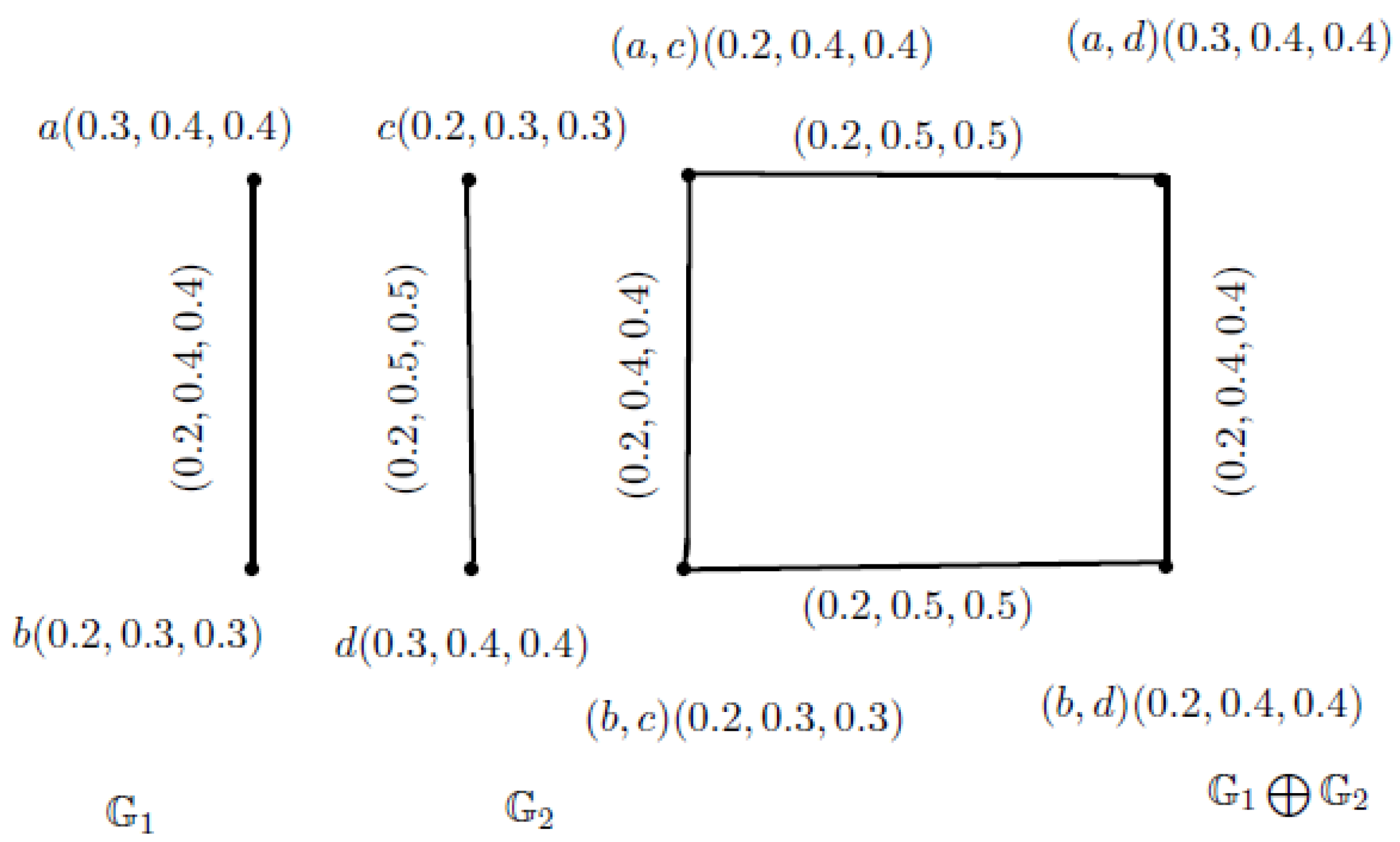
Definition 8.

The RJ ${\mathbb{G}}_1|{\mathbb{G}}_2=(U_1|U_2,W_1\left|W_2\right)$ of two PFGs ${\mathbb{G}}_1=(U_1,W_1)$ and ${\mathbb{G}}_2=(U_2,W_2)$ is defined as:

(i)

$$\begin{array}{cc}\hfill & \left({\chi }_{U_1}\right|{\chi }_{U_2})\left((u_1,u_2)\right)=\wedge \{{\chi }_{U_1}\left(u_1\right),{\chi }_{U_2}\left(u_2\right)\},\hfill \end{array}$$

$$\begin{array}{cc}\hfill & \left({\varphi }_{U_1}\right|{\varphi }_{U_2})\left((u_1,u_2)\right)=\wedge \{{\varphi }_{U_1}\left(u_1\right),{\varphi }_{U_2}\left(u_2\right)\},\hfill \end{array}$$

$$\begin{array}{cc}\hfill & \left({\psi }_{U_1}\right|{\psi }_{U_2})\left((u_1,u_2)\right)=\vee \{{\psi }_{U_1}\left(u_1\right),{\psi }_{U_2}\left(u_2\right)\}.\hfill \end{array}$$

$\forall (u_1,u_2)\in (V_1\times V_2)$,

(ii)

$$\begin{array}{cc}\hfill & \left({\chi }_{W_1}\right|{\chi }_{W_2})\left((m,u_2)(m,w_2)\right)=\wedge \{{\chi }_{U_1}\left(m\right),{\chi }_{U_2}\left(u_2\right),{\chi }_{U_2}\left(w_2\right)\},\hfill \end{array}$$

$$\begin{array}{cc}\hfill & \left({\varphi }_{W_1}\right|{\varphi }_{W_2})\left((m,u_2)(m,w_2)\right)=\wedge \{{\varphi }_{U_1}\left(m\right),{\varphi }_{U_2}\left(u_2\right),{\varphi }_{U_2}\left(w_2\right)\},\hfill \end{array}$$

$$\begin{array}{cc}\hfill & \left({\psi }_{W_1}\right|{\psi }_{W_2})\left((m,u_2)(m,w_2)\right)=\vee \{{\psi }_{U_1}\left(m\right),{\psi }_{U_2}\left(u_2\right),{\psi }_{U_2}\left(w_2\right)\},\hfill \end{array}$$

$\forall m\in V_{2}and{u}_2{w}_2\notin E_2$.

(iii)

$$\begin{array}{cc}\hfill & \left({\chi }_{W_1}\right|{\chi }_{W_2})\left((m,u_2)(m,w_2)\right)=\wedge \{{\chi }_{U_1}\left(m\right),{\chi }_{U_2}\left(u_2\right),{\chi }_{U_2}\left(w_2\right)\},\hfill \end{array}$$

$$\begin{array}{cc}\hfill & \left({\varphi }_{W_1}\right|{\varphi }_{W_2})\left((m,u_2)(m,w_2)\right)=\wedge \{{\varphi }_{U_1}\left(m\right),{\varphi }_{U_2}\left(u_2\right),{\varphi }_{U_2}\left(w_2\right)\},\hfill \end{array}$$

$$\begin{array}{cc}\hfill & \left({\psi }_{W_1}\right|{\psi }_{W_2})\left((m,u_2)(m,w_2)\right)=\vee \{{\psi }_{U_1}\left(m\right),{\psi }_{U_2}\left(u_2\right),{\psi }_{U_2}\left(w_2\right)\},\hfill \end{array}$$

$\forall z\in V_{2}and{u}_1{w}_1\notin E_1$.

(iv)

$$\begin{array}{cc}\hfill & \left({\chi }_{W_1}\right|{\chi }_{W_2})\left((u_1,u_2)(w_1,w_2)\right)=\wedge \{{\chi }_{U_1}\left(u_1\right),{\chi }_{U_1}\left(w_1\right),{\chi }_{U_2}\left(u_2\right),{\chi }_{U_2}\left(w_2\right)\},\hfill \end{array}$$

$$\begin{array}{cc}\hfill & \left({\varphi }_{W_1}\right|{\varphi }_{W_2})\left((u_1,u_2)(w_1,w_2)\right)=\wedge \{{\varphi }_{U_1}\left(u_1\right),{\varphi }_{U_1}\left(w_1\right),{\varphi }_{U_2}\left(u_2\right),{\varphi }_{W_2}\left(w_2\right)\},\hfill \end{array}$$

$$\begin{array}{cc}\hfill & \left({\psi }_{W_1}\right|{\psi }_{W_2})\left((u_1,u_2)(w_1,w_2)\right)=\vee \{{\psi }_{U_1}\left(u_1\right),{\psi }_{U_1}\left(w_1\right),{\psi }_{U_2}\left(u_2\right),{\psi }_{U_2}\left(w_2\right)\},\hfill \end{array}$$

$\forall u_1{w}_1\notin E_1$ and $u_2{w}_2\notin E_2$.

Example 7.

Suppose that ${\mathbb{G}}_1$ and ${\mathbb{G}}_2$ are two PFGs, as in Figure 10 and Figure 11. We can see the RJ of the two PFGs ${\mathbb{G}}_1$ and ${\mathbb{G}}_2$, that is, ${\mathbb{G}}_1|{\mathbb{G}}_2$, in Figure 12.

For node $(e,a)$, we calculate Mv, IDv, and NMv as follows:

$$\begin{array}{ccc}& & \left({\chi }_{U_1}\right|{\chi }_{U_2})(e,a)=\wedge \{{\chi }_{U_1}\left(e\right),{\chi }_{U_2}\left(a\right)\}\hfill \\ & & =\wedge \{0.1,0.1\}=0.1,\hfill \\ & & \left({\varphi }_{U_1}\right|{\varphi }_{U_2})(e,a)=\wedge \{{\varphi }_{U_1}\left(e\right),{\varphi }_{U_2}\left(a\right)\}\hfill \\ & & =\wedge \{0.3,0.2\}=0.2,\hfill \\ & & \left({\psi }_{U_1}\right|{\psi }_{U_2})(e,a)=\vee \{{\psi }_{U_1}\left(e\right),{\psi }_{U_2}\left(a\right)\}\hfill \\ & & =\vee \{0.2,0.3\}=0.3\hfill \end{array}$$

for $a\in V_1$ and $e\in V_2$.

For arc $(e,c)(e,a)$, we calculate Mv, IDv, and NMv as follows.

$$\begin{array}{ccc}& & \left({\chi }_{W_1}\right|{\chi }_{W_2})\left((e,c)(e,a)\right)=\wedge \{{\chi }_{U_1}\left(e\right),{\chi }_{U_2}\left(c\right),{\chi }_{U_2}\left(a\right)\}\hfill \\ & & =\wedge \{0.1,0.1,0.1\}=0.1,\hfill \\ & & \left({\varphi }_{W_1}\right|{\varphi }_{W_2})\left((e,c)(e,a)\right)=\wedge \{{\varphi }_{U_1}\left(e\right),{\varphi }_{U_2}\left(c\right),{\varphi }_{U_2}\left(a\right)\}\hfill \\ & & =\wedge \{0.3,0.2,0.2\}=0.2,\hfill \\ & & \left({\psi }_{W_1}\right|{\psi }_{W_2})\left((e,c)(e,a)\right)=\vee \{{\psi }_{U_1}\left(e\right),{\psi }_{U_2}\left(c\right),{\psi }_{U_2}\left(a\right)\}\hfill \\ & & =\vee \{0.2,0.3,0.3\}=0.3\hfill \end{array}$$

for $e\in V_2$ and $ac\notin E_1$.

We can calculate Mv, IDv, and NMv for all other nodes and edges.

Proposition 2.

The RJ of two PFGs ${\mathbb{G}}_1$ and ${\mathbb{G}}_2$ is a PFG.

Proof. 

Suppose that ${\mathbb{G}}_1=(U_1,W_1)$ and ${\mathbb{G}}_2=(U_2,W_2)$ are two PFGs on crisp graphs $G_1=(V_1,E_1)$ and $G_2=(V_2,E_2)$, respectively, and $\left((u_1,u_2)(w_1,w_2)\right)\in E_1\times E_2$. Then, by Definition 8, we have:

(i) If $u_1=w_1,u_2{w}_2\notin E_2$,

$$\begin{array}{cc}\hfill \left({\chi }_{W_1}\right|{\chi }_{W_2})\left((u_1,u_2)(w_1,w_2)\right)& =\wedge \{{\chi }_{U_1}\left(u_1\right),{\chi }_{U_2}\left(u_2\right),{\chi }_{U_2}\left(w_2\right)\}\hfill \\ \hfill & =\wedge \{\wedge \{{\chi }_{U_1}\left(u_1\right),{\chi }_{U_2}\left(u_2\right)\},\wedge \{{\chi }_{U_1}\left(w_1\right),{\chi }_{U_2}\left(w_2\right)\}\}\hfill \\ \hfill & =\wedge \{\left({\chi }_{U_1}\right|{\chi }_{U_2})(u_1,u_2),\left({\chi }_{U_1}\right|{\chi }_{U_2})(w_1,w_2)\},\hfill \end{array}$$

$$\begin{array}{cc}\hfill \left({\varphi }_{W_1}\right|{\varphi }_{W_2})\left((u_1,u_2)(w_1,w_2)\right)& =\wedge \{{\varphi }_{U_1}\left(u_1\right),{\varphi }_{U_2}\left(u_2\right),{\varphi }_{U_2}\left(w_2\right)\}\hfill \\ \hfill & =\wedge \{\wedge \{{\varphi }_{U_1}\left(u_1\right),{\varphi }_{U_2}\left(u_2\right)\},\wedge \{{\varphi }_{U_1}\left(w_1\right),{\varphi }_{U_2}\left(w_2\right)\}\}\hfill \\ \hfill & =\wedge \{\left({\varphi }_{U_1}\right|{\varphi }_{U_2})(u_1,u_2),\left({\varphi }_{U_1}\right|{\varphi }_{U_2})(w_1,w_2)\},\hfill \end{array}$$

$$\begin{array}{cc}\hfill \left({\psi }_{W_1}\right|{\psi }_{W_2})\left((u_1,u_2)(w_1,w_2)\right)& =\vee \{{\psi }_{U_1}\left(u_1\right),{\psi }_{U_2}\left(u_2\right),{\psi }_{U_2}\left(w_2\right)\}\hfill \\ \hfill & =\vee \{\vee \{{\psi }_{U_1}\left(u_1\right),{\psi }_{U_2}\left(u_2\right)\},\vee \{{\psi }_{U_1}\left(w_1\right),{\psi }_{U_2}\left(w_2\right)\}\}\hfill \\ \hfill & =\vee \{\left({\psi }_{U_1}\right|{\psi }_{U_2})(u_1,u_2),\left({\psi }_{U_1}\right|{\psi }_{U_2})(w_1,w_2)\}.\hfill \end{array}$$

(ii) If $u_2=w_2,u_1{w}_1\notin E_1$,

$$\begin{array}{cc}\hfill \left({\chi }_{W_1}\right|{\chi }_{W_2})\left((u_1,u_2)(w_1,w_2)\right)& =\wedge \{{\chi }_{U_1}\left(u_1\right),{\chi }_{U_1}\left(w_1\right),{\chi }_{U_2}\left(u_2\right)\}\hfill \\ \hfill & =\wedge \{\wedge \{{\chi }_{U_1}\left(u_1\right),{\chi }_{U_2}\left(u_2\right)\},\wedge \{{\chi }_{U_1}\left(w_1\right),{\chi }_{U_2}\left(w_2\right)\}\}\hfill \\ \hfill & =\wedge \{\left({\chi }_{U_1}\right|{\chi }_{U_2})(u_1,u_2),\left({\chi }_{U_1}\right|{\chi }_{U_2})(w_1,w_2)\},\hfill \end{array}$$

$$\begin{array}{cc}\hfill \left({\varphi }_{W_1}\right|{\varphi }_{W_2})\left((u_1,u_2)(w_1,w_2)\right)& =\wedge \{{\varphi }_{U_1}\left(u_1\right),{\varphi }_{U_1}\left(w_1\right),{\varphi }_{U_2}\left(u_2\right)\}\hfill \\ \hfill & =\wedge \{\wedge \{{\varphi }_{U_1}\left(u_1\right),{\varphi }_{U_2}\left(u_2\right)\},\wedge \{{\varphi }_{U_1}\left(w_1\right),{\varphi }_{U_2}\left(w_2\right)\}\}\hfill \\ \hfill & =\wedge \{\left({\varphi }_{U_1}\right|{\varphi }_{U_2})(u_1,u_2),\left({\varphi }_{U_1}\right|{\varphi }_{U_2})(w_1,w_2)\},\hfill \end{array}$$

$$\begin{array}{cc}\hfill \left({\psi }_{W_1}\right|{\psi }_{W_2})\left((u_1,u_2)(w_1,w_2)\right)& =\vee \{{\psi }_{U_1}\left(u_1\right),{\psi }_{U_1}\left(w_1\right),{\psi }_{U_2}\left(u_2\right)\}\hfill \\ \hfill & =\vee \{\vee \{{\psi }_{U_1}\left(u_1\right),{\psi }_{U_2}\left(u_2\right)\},\vee \{{\psi }_{U_1}\left(w_1\right),{\psi }_{U_2}\left(w_2\right)\}\}\hfill \\ \hfill & =\vee \{\left({\psi }_{U_1}\right|{\psi }_{U_2})(u_1,u_2),\left({\psi }_{U_1}\right|{\psi }_{U_2})(w_1,w_2)\}.\hfill \end{array}$$

(iii) If $u_1{w}_1\notin E_{1}and{u}_2{w}_2\notin E_2$,

$$\begin{array}{cc}\hfill \left({\chi }_{W_1}\right|{\chi }_{W_2})\left((u_1,u_2)(w_1,w_2)\right)& =\wedge \{{\chi }_{U_1}\left(u_1\right),{\chi }_{U_1}\left(w_1\right),{\chi }_{U_2}\left(u_2\right),{\chi }_{U_2}\left(w_2\right)\}\hfill \\ \hfill & =\wedge \{\wedge \{{\chi }_{U_1}\left(u_1\right),{\chi }_{U_2}\left(u_2\right)\},\wedge \{{\chi }_{U_1}\left(w_1\right),{\chi }_{U_2}\left(w_2\right)\}\}\hfill \\ \hfill & =\wedge \{\left({\chi }_{U_1}\right|{\chi }_{U_2})(u_1,u_2),\left({\chi }_{U_1}\right|{\chi }_{U_2})(w_1,w_2)\},\hfill \end{array}$$

$$\begin{array}{cc}\hfill \left({\varphi }_{W_1}\right|{\varphi }_{W_2})\left((u_1,u_2)(w_1,w_2)\right)& =\wedge \{{\varphi }_{U_1}\left(u_1\right),{\varphi }_{U_1}\left(w_1\right),{\varphi }_{U_2}\left(u_2\right),{\chi }_{U_2}\left(w_2\right)\}\hfill \\ \hfill & =\wedge \{\wedge \{{\varphi }_{U_1}\left(u_1\right),{\varphi }_{U_2}\left(u_2\right)\},\wedge \{{\varphi }_{U_1}\left(w_1\right),{\varphi }_{U_2}\left(w_2\right)\}\}\hfill \\ \hfill & =\wedge \{\left({\varphi }_{U_1}\right|{\varphi }_{U_2})(u_1,u_2),\left({\varphi }_{U_1}\right|{\varphi }_{U_2})(w_1,w_2)\},\hfill \end{array}$$

$$\begin{array}{cc}\hfill \left({\psi }_{W_1}\right|{\psi }_{W_2})\left((u_1,u_2)(w_1,w_2)\right)& =\vee \{{\psi }_{U_1}\left(u_1\right),{\psi }_{U_1}\left(w_1\right),{\psi }_{U_2}\left(u_2\right),{\psi }_{U_2}\left(w_2\right)\}\hfill \\ \hfill & =\vee \{\vee \{{\psi }_{U_1}\left(u_1\right),{\psi }_{U_2}\left(u_2\right)\},\vee \{{\psi }_{U_1}\left(w_1\right),{\psi }_{U_2}\left(w_2\right)\}\}\hfill \\ \hfill & =\vee \{\left({\psi }_{U_1}\right|{\psi }_{U_2})(u_1,u_2),\left({\psi }_{U_1}\right|{\psi }_{U_2})(w_1,w_2)\}.\hfill \end{array}$$

Therefore, ${\mathbf{G}}_1|{\mathbf{G}}_2=(U_1|U_2,W_1\left|W_2\right)$ is a PFG. □

Remark 3.

The RJ of two complete PFGs ${\mathbf{G}}_1=(U_1,W_1)$ and ${\mathbf{G}}_2=(U_2,W_2)$ is a complete PFG.

Definition 9.

Suppose that ${\mathbf{G}}_1=(U_1,W_1)$ and ${\mathbf{G}}_2=(U_2,W_2)$ are two PFGs. For any node $(u_1,u_2)\in V_1\times V_2$, we have:

$$\begin{array}{cc}\hfill {\left(d_{\chi }\right)}_{{\mathbb{G}}_1|{\mathbb{G}}_2}(u_1,u_2)& =\sum _{(u_1,u_2)(w_1,w_2)\in E_1\times E_2.}\left({\chi }_{W_1}\right|{\chi }_{W_2})\left((u_1,u_2)(w_1,w_2)\right)\hfill \\ \hfill & =\sum _{u_1=w_1,u_2{w}_2\notin E_2}\wedge \{{\chi }_{U_1}\left(u_1\right),{\chi }_{U_2}\left(u_2\right),{\chi }_{U_2}\left(w_2\right)\}\hfill \\ \hfill & +\sum _{u_2=w_2,u_1{w}_1\notin E_1}\wedge \{{\chi }_{U_1}\left(u_1\right),{\chi }_{U_1}\left(w_1\right),{\chi }_{U_2}\left(u_2\right)\}\hfill \\ \hfill & +\sum _{u_1{w}_1\notin E_{1}and{u}_2{w}_2\notin E_2}\wedge \{{\chi }_{U_1}\left(u_1\right),{\chi }_{U_1}\left(w_1\right),{\chi }_{U_2}\left(u_2\right),{\chi }_{U_2}\left(w_2\right)\},\hfill \end{array}$$

$$\begin{array}{cc}\hfill {\left(d_{\varphi }\right)}_{{\mathbb{G}}_1|{\mathbb{G}}_2}(u_1,u_2)& =\sum _{(u_1,u_2)(w_1,w_2)\in E_1\times E_2.}\left({\varphi }_{W_1}\right|{\varphi }_{W_2})\left((u_1,u_2)(w_1,w_2)\right)\hfill \\ \hfill & =\sum _{u_1=w_1,u_2{w}_2\notin E_2}\wedge \{{\varphi }_{U_1}\left(u_1\right),{\varphi }_{U_2}\left(u_2\right),{\varphi }_{U_2}\left(w_2\right)\}\hfill \\ \hfill & +\sum _{u_2=w_2,u_1{w}_1\notin E_1}\wedge \{{\varphi }_{U_1}\left(u_1\right),{\varphi }_{U_1}\left(w_1\right),{\varphi }_{U_2}\left(u_2\right)\}\hfill \\ \hfill & +\sum _{u_1{w}_1\notin E_{1}and{u}_2{w}_2\notin E_2}\wedge \{{\varphi }_{U_1}\left(u_1\right),{\varphi }_{U_1}\left(w_1\right),{\varphi }_{U_2}\left(u_2\right),{\varphi }_{U_2}\left(w_2\right)\},\hfill \end{array}$$

$$\begin{array}{cc}\hfill {\left(d_{\psi }\right)}_{{\mathbb{G}}_1|{\mathbb{G}}_2}(u_1,u_2)& =\sum _{(u_1,u_2)(w_1,w_2)\in E_1\times E_2.}\left({\psi }_{W_1}\right|{\psi }_{W_2})\left((u_1,u_2)(w_1,w_2)\right)\hfill \\ \hfill & =\sum _{u_1=w_1,u_2{w}_2\notin E_2}\vee \{{\psi }_{U_1}\left(u_1\right),{\psi }_{U_2}\left(u_2\right),{\psi }_{U_2}\left(w_2\right)\}\hfill \\ \hfill & +\sum _{u_2=w_2,u_1{w}_1\notin E_1}\vee \{{\psi }_{U_1}\left(u_1\right),{\psi }_{U_1}\left(w_1\right),{\psi }_{U_2}\left(u_2\right)\}\hfill \\ \hfill & +\sum _{u_1{w}_1\notin E_{1}and{u}_2{w}_2\notin E_2}\vee \{{\psi }_{U_1}\left(u_1\right),{\psi }_{U_1}\left(w_1\right),{\psi }_{U_2}\left(u_2\right),{\psi }_{U_2}\left(w_2\right)\}.\hfill \end{array}$$

Definition 10.

Suppose that ${\mathbb{G}}_1=(U_1,W_1)$ and ${\mathbb{G}}_2=(U_2,Y_2)$ are two PFGs. $\forall (u_1,u_2)\in V_1\times V_2$,

$$\begin{array}{cc}\hfill {\left(t{d}_{\chi }\right)}_{{\mathbb{G}}_1|{\mathbb{G}}_2}(u_1,u_2)& =\sum _{(u_1,u_2)(w_1,w_2)\in E_1\times E_2.}\left({\chi }_{W_1}\right|{\chi }_{W_2})\left((u_1,u_2)(w_1,w_2)\right)+\left({\chi }_{U_1}\right|{\chi }_{U_2})(u_1,u_2)\hfill \\ \hfill & =\sum _{u_1=w_1,u_2{w}_2\notin E_2}\wedge \{{\chi }_{U_1}\left(u_1\right),{\chi }_{U_2}\left(u_2\right),{\chi }_{U_2}\left(w_2\right)\}\hfill \\ \hfill & +\sum _{u_2=w_2,u_1{w}_1\notin E_1}\wedge \{{\chi }_{U_1}\left(u_1\right),{\chi }_{U_1}\left(w_1\right),{\chi }_{U_2}\left(u_2\right)\}\hfill \\ \hfill & +\sum _{u_1{w}_1\notin E_{1}and{u}_2{w}_2\notin E_2}\wedge \{{\chi }_{U_1}\left(u_1\right),{\chi }_{U_1}\left(w_1\right),{\chi }_{U_2}\left(u_2\right),{\chi }_{U_2}\left(w_2\right)\},\hfill \end{array}$$

$$\begin{array}{cc}\hfill {\left(t{d}_{\varphi }\right)}_{{\mathbb{G}}_1|{\mathbb{G}}_2}(u_1,u_2)& =\sum _{(u_1,u_2)(w_1,w_2)\in E_1\times E_2.}\left({\varphi }_{W_1}\right|{\varphi }_{W_2})\left((u_1,u_2)(w_1,w_2)\right)+\left({\varphi }_{U_1}\right|{\varphi }_{U_2})(u_1,u_2)\hfill \\ \hfill & =\sum _{u_1=w_1,u_2{w}_2\notin E_2}\wedge \{{\varphi }_{U_1}\left(u_1\right),{\varphi }_{U_2}\left(u_2\right),{\varphi }_{U_2}\left(w_2\right)\}\hfill \\ \hfill & +\sum _{u_2=w_2,u_1{w}_1\notin E_1}\wedge \{{\varphi }_{U_1}\left(u_1\right),{\varphi }_{U_1}\left(w_1\right),{\varphi }_{U_2}\left(u_2\right)\}\hfill \\ \hfill & +\sum _{u_1{w}_1\notin E_{1}and{u}_2{w}_2\notin E_2}\wedge \{{\varphi }_{U_1}\left(u_1\right),{\varphi }_{U_1}\left(w_1\right),{\varphi }_{U_2}\left(u_2\right),{\varphi }_{U_2}\left(w_2\right)\},\hfill \end{array}$$

$$\begin{array}{cc}\hfill {\left(t{d}_{\psi }\right)}_{{\mathbb{G}}_1|{\mathbb{G}}_2}(u_1,u_2)& =\sum _{(u_1,u_2)(w_1,w_2)\in E_1\times E_2.}\left({\psi }_{W_1}\right|{\psi }_{W_2})\left((u_1,u_2)(w_1,w_2)\right)+\left({\psi }_{U_1}\right|{\psi }_{U_2})(u_1,u_2)\hfill \\ \hfill & =\sum _{u_1=w_1,u_2{w}_2\notin E_2}\vee \{{\psi }_{U_1}\left(u_1\right),{\psi }_{U_2}\left(u_2\right),{\psi }_{U_2}\left(w_2\right)\}\hfill \\ \hfill & +\sum _{u_2=w_2,u_1{w}_1\notin E_1}\vee \{{\psi }_{U_1}\left(u_1\right),{\psi }_{U_1}\left(w_1\right),{\psi }_{U_2}\left(u_2\right)\}\hfill \\ \hfill & +\sum _{u_1{w}_1\notin E_{1}and{u}_2{w}_2\notin E_2}\vee \{{\psi }_{U_1}\left(u_1\right),{\psi }_{U_1}\left(w_1\right),{\psi }_{U_2}\left(u_2\right),{\psi }_{U_2}\left(w_2\right)\}.\hfill \end{array}$$

Example 8.

We calculate the degree and the total degree of node $(d,a)$ in Example 7.

$$\begin{array}{cc}\hfill {\left(d_{\chi }\right)}_{{\mathbb{G}}_1|{\mathbb{G}}_2}(d,a)& =\wedge \{{\chi }_{U_2}\left(d\right),{\chi }_{U_1}\left(a\right),{\chi }_{U_1}\left(c\right)\}+\wedge \{{\chi }_{U_2}\left(d\right),{\chi }_{U_1}\left(a\right),{\chi }_{U_2}\left(f\right),{\chi }_{U_1}\left(c\right)\}\hfill \\ \hfill & +\wedge \{{\chi }_{U_2}\left(d\right),{\chi }_{U_1}\left(a\right),{\chi }_{U_2}\left(g\right),{\chi }_{U_1}\left(c\right)\}\hfill \\ \hfill & =\wedge \{0.1,0.1,0.1\}+\wedge \{0.1,0.1,0.2,0.1\}+\wedge \{0.1,0.1,0.1,0.1\}\hfill \\ \hfill & =0.1+0.1+0.1\hfill \\ \hfill & =0.3,\hfill \end{array}$$

$$\begin{array}{cc}\hfill {\left(d_{\varphi }\right)}_{{\mathbb{G}}_1|{\mathbb{G}}_2}(d,a)& =\wedge \{{\varphi }_{U_2}\left(d\right),{\varphi }_{U_1}\left(a\right),{\varphi }_{U_1}\left(c\right)\}+\wedge \{{\varphi }_{U_2}\left(d\right),{\varphi }_{U_1}\left(a\right),{\varphi }_{U_2}\left(f\right),{\varphi }_{U_1}\left(c\right)\}\hfill \\ \hfill & +\wedge \{{\varphi }_{U_2}\left(d\right),{\varphi }_{U_1}\left(a\right),{\varphi }_{U_2}\left(g\right),{\varphi }_{U_1}\left(c\right)\}\hfill \\ \hfill & =\wedge \{0.2,0.2,0.2\}+\wedge \{0.2,0.2,0.2,0.2\}+\wedge \{0.2,0.2,0.3,0.2\}\hfill \\ \hfill & =0.2+0.2+0.2\hfill \\ \hfill & =0.6,\hfill \end{array}$$

$$\begin{array}{cc}\hfill {\left(d_{\psi }\right)}_{{\mathbb{G}}_1|{\mathbb{G}}_2}(d,a)& =\vee \{{\psi }_{U_2}\left(d\right),{\psi }_{U_1}\left(a\right),{\psi }_{U_1}\left(c\right)\}+\vee \{{\psi }_{U_2}\left(d\right),{\psi }_{U_1}\left(a\right),{\psi }_{U_2}\left(f\right),{\psi }_{U_1}\left(c\right)\}\hfill \\ \hfill & +\vee \{{\psi }_{U_2}\left(d\right),{\psi }_{U_1}\left(a\right),{\psi }_{U_2}\left(g\right),{\psi }_{U_1}\left(c\right)\}\hfill \\ \hfill & =\vee \{0.2,0.3,0.3\}+\vee \{0.2,0.3,0.3,0.3\}+\vee \{0.2,0.3,0.3,0.3\}\hfill \\ \hfill & =0.3+0.3+0.3\hfill \\ \hfill & =1.3.\hfill \end{array}$$

Hence, $d_{{\mathbb{G}}_1|{\mathbb{G}}_2}(a,c)$= (0.3,1.0, 1.3).

For the total vertex degree,

$$\begin{array}{cc}\hfill {\left(t{d}_{\chi }\right)}_{{\mathbb{G}}_1|{\mathbb{G}}_2}(d,a)& =\wedge \{{\chi }_{U_2}\left(d\right),{\chi }_{U_1}\left(a\right),{\chi }_{U_1}\left(c\right)\}+\wedge \{{\chi }_{U_2}\left(d\right),{\chi }_{U_1}\left(a\right),{\chi }_{U_2}\left(f\right),{\chi }_{U_1}\left(c\right)\}\hfill \\ \hfill & +\wedge \{{\chi }_{U_2}\left(d\right),{\chi }_{U_1}\left(a\right),{\chi }_{U_2}\left(g\right),{\chi }_{U_1}\left(c\right)\}+\wedge \{{\chi }_{U_2}\left(d\right),{\chi }_{U_1}\left(a\right)\}\hfill \\ \hfill & =\wedge \{0.1,0.1,0.1\}+\wedge \{0.1,0.1,0.2,0.1\}+\wedge \{0.1,0.1,0.1,0.1\}+\wedge \{0.1,0.1\}\hfill \\ \hfill & =0.1+0.1+0.1+0.1\hfill \\ \hfill & =0.4,\hfill \end{array}$$

$$\begin{array}{cc}\hfill {\left(t{d}_{\varphi }\right)}_{{\mathbb{G}}_1|{\mathbb{G}}_2}(d,a)& =\vee \{{\varphi }_{U_2}\left(d\right),{\varphi }_{U_1}\left(a\right),{\varphi }_{U_1}\left(c\right)\}+\vee \{{\varphi }_{U_2}\left(d\right),{\varphi }_{U_1}\left(a\right),{\varphi }_{U_2}\left(f\right),{\varphi }_{U_1}\left(c\right)\}\hfill \\ \hfill & +\vee \{{\varphi }_{U_2}\left(d\right),{\varphi }_{U_1}\left(a\right),{\varphi }_{U_2}\left(g\right),{\varphi }_{U_1}\left(c\right)\}+\vee \{{\varphi }_{U_2}\left(d\right),{\varphi }_{U_1}\left(a\right)\}\hfill \\ \hfill & =\vee \{0.2,0.2,0.2\}+\vee \{0.2,0.2,0.2,0.2\}+\vee \{0.2,0.2,0.3,0.2\}+\vee \{0.2,0.2\}\hfill \\ \hfill & =0.2+0.2+0.2+0.2\hfill \\ \hfill & =0.8,\hfill \end{array}$$

$$\begin{array}{cc}\hfill {\left(t{d}_{\psi }\right)}_{{\mathbb{G}}_1|{\mathbb{G}}_2}(d,a)& =\vee \{{\psi }_{U_2}\left(d\right),{\psi }_{U_1}\left(a\right),{\psi }_{U_1}\left(c\right)\}+\vee \{{\psi }_{U_2}\left(d\right),{\psi }_{U_1}\left(a\right),{\psi }_{U_2}\left(f\right),{\psi }_{U_1}\left(c\right)\}\hfill \\ \hfill & +\vee \{{\psi }_{U_2}\left(d\right),{\psi }_{U_1}\left(a\right),{\psi }_{U_2}\left(g\right),{\psi }_{U_1}\left(c\right)\}+\vee \{{\psi }_{U_2}\left(d\right),{\psi }_{U_1}\left(a\right)\}\hfill \\ \hfill & =\vee \{0.2,0.3,0.3\}+\vee \{0.2,0.3,0.3,0.3\}+\vee \{0.2,0.3,0.3,0.3\}+\vee \{0.2,0.3\}\hfill \\ \hfill & =0.3+0.3+0.3+0.3\hfill \\ \hfill & =1.2.\hfill \end{array}$$

Hence, $t{d}_{{\mathbb{G}}_1|{\mathbb{G}}_2}(a,c)$= (0.4, 1.3, 1.7).

We can calculate the degree and the total degree of all nodes in ${\mathbb{G}}_1|{\mathbb{G}}_2$ in the same way.

Definition 11.

The SD ${\mathbb{G}}_1\oplus {\mathbb{G}}_2=(U_1\oplus U_2,W_1\oplus W_2)$ of two PFGs ${\mathbb{G}}_1=(U_1,W_1)$ and ${\mathbb{G}}_2=(U_2,W_2)$ is defined as:

(i)

$$\begin{array}{cc}\hfill & ({\chi }_{U_1}\oplus {\chi }_{U_2})(u_1,u_2)=\wedge \{{\chi }_{U_1}\left(u_1\right),{\chi }_{U_2}\left(u_2\right)\},\hfill \end{array}$$

$$\begin{array}{cc}\hfill & ({\varphi }_{U_1}\oplus {\varphi }_{U_2})(u_1,u_2)=\wedge \{{\varphi }_{U_1}\left(u_1\right),{\varphi }_{U_2}\left(u_2\right)\},\hfill \end{array}$$

$$\begin{array}{cc}\hfill & ({\psi }_{U_1}\oplus {\psi }_{U_2})(u_1,u_2)=\vee \{{\psi }_{U_1}\left(u_1\right),{\psi }_{U_2}\left(u_2\right)\}.\hfill \end{array}$$

$\forall (u_1,u_2)\in (V_1\times V_2)$.

(ii)

$$\begin{array}{cc}\hfill & ({\chi }_{W_1}\oplus {\chi }_{W_2})\left((m,u_2)(m,w_2)\right)=\wedge \{{\chi }_{U_1}\left(m\right),{\chi }_{W_2}\left(u_2{w}_2\right)\},\hfill \end{array}$$

$$\begin{array}{cc}\hfill & ({\varphi }_{W_1}\oplus {\varphi }_{W_2})\left((m,u_2)(m,w_2)\right)=\wedge \{{\varphi }_{U_1}\left(m\right),{\varphi }_{W_2}\left(u_2{w}_2\right)\},\hfill \end{array}$$

$$\begin{array}{cc}\hfill & ({\psi }_{W_1}\oplus {\psi }_{W_2})\left((m,u_2)(m,w_2)\right)=\vee \{{\psi }_{U_1}\left(m\right),{\psi }_{W_2}\left(u_2{w}_2\right)\}.\hfill \end{array}$$

$\forall m\in V_{1}and{u}_2{w}_2\in E_2$.

(iii)

$$\begin{array}{cc}\hfill & ({\chi }_{W_1}\oplus {\chi }_{W_2})\left((u_1,z)(w_1,z)\right)=\wedge \{{\chi }_{W_1}\left(u_1{w}_1\right),{\chi }_{U_2}\left(z\right)\},\hfill \end{array}$$

$$\begin{array}{cc}\hfill & ({\varphi }_{W_1}\oplus {\varphi }_{W_2})\left((u_1,z)(w_1,z)\right)=\wedge \{{\varphi }_{W_1}\left(u_1{w}_1\right),{\varphi }_{U_2}\left(z\right)\},\hfill \end{array}$$

$$\begin{array}{cc}\hfill & ({\psi }_{W_1}\oplus {\psi }_{W_2})\left((u_1,z)(w_1,z)\right)=\vee \{{\psi }_{W_1}\left(u_1{w}_1\right),{\psi }_{U_2}\left(z\right)\}.\hfill \end{array}$$

$\forall z\in V_{2}and{u}_1{w}_1\in E_1$.

(iv)

$$\begin{array}{cc}\hfill ({\chi }_{W_1}\oplus {\chi }_{W_2})\left((u_1,u_2)(w_1,w_2)\right)& =\wedge \{{\chi }_{U_1}\left(u_1\right),{\chi }_{U_1}\left(w_1\right),{\chi }_{W_2}\left(u_2{w}_2\right)\}\hfill \\ \hfill for all{u}_1{w}_1\notin E_{1}and{u}_2{w}_2\in E_2,\\ \hfill & or\hfill \\ \hfill & =\wedge \{{\chi }_{U_2}\left(u_2\right),{\chi }_{U_2}\left(w_2\right),{\chi }_{W_1}\left(u_1{w}_1\right)\}\hfill \\ \hfill for all{u}_1{w}_1\in E_{1}and{u}_2{w}_2\notin E_2.\end{array}$$

$$\begin{array}{cc}\hfill ({\varphi }_{W_1}\oplus {\varphi }_{W_2})\left((u_1,u_2)(w_1,w_2)\right)& =\wedge \{{\varphi }_{U_1}\left(u_1\right),{\varphi }_{U_1}\left(w_1\right),{\varphi }_{W_2}\left(u_2{w}_2\right)\}\hfill \\ \hfill for all{u}_1{w}_1\notin E_{1}and{u}_2{w}_2\in E_2,\\ \hfill & or\hfill \\ \hfill & =\wedge \{{\varphi }_{U_2}\left(u_2\right),{\varphi }_{U_2}\left(w_2\right),{\varphi }_{W_1}\left(u_1{w}_1\right)\}\hfill \\ \hfill for all{u}_1{w}_1\in E_{1}and{u}_2{w}_2\notin E_2.\end{array}$$

$$\begin{array}{cc}\hfill ({\psi }_{W_1}\oplus {\psi }_{W_2})\left((u_1,u_2)(w_1,w_2)\right)& =\vee \{{\psi }_{U_1}\left(u_1\right),{\psi }_{U_1}\left(w_1\right),{\psi }_{W_2}\left(u_2{w}_2\right)\}\hfill \\ \hfill for all{u}_1{w}_1\notin E_{1}and{u}_2{w}_2\in E_2,\\ \hfill & or\hfill \\ \hfill & =\vee \{{\psi }_{U_2}\left(u_2\right),{\psi }_{U_2}\left(w_2\right),{\psi }_{W_2}\left(u_1{w}_1\right)\}\hfill \\ \hfill for all{u}_1{w}_1\in E_{1}and{u}_2{w}_2\notin E_2.\end{array}$$

Example 9.

Taking ${\mathbb{G}}_1$ and ${\mathbb{G}}_2$ as PFGs, as shown in Figure 13 and Figure 14, we can see the SD of the two PFGs ${\mathbb{G}}_1$ and ${\mathbb{G}}_2$, that is, ${\mathbb{G}}_1\oplus {\mathbb{G}}_2$, in Figure 15.

For node $(a,f)$, we calculate Mv, IDv, and NMv as follows:

$$\begin{array}{ccc}& & ({\chi }_{U_1}\oplus {\chi }_{U_2})(a,f)=\wedge \{{\chi }_{U_1}\left(a\right),{\chi }_{U_2}\left(f\right)\}\hfill \\ & & =\wedge \{0.2,0.4\}=0.2,\hfill \\ & & ({\varphi }_{U_1}\oplus {\varphi }_{U_2})(a,f)=\vee \{{\varphi }_{U_1}\left(a\right),{\varphi }_{U_2}\left(f\right)\}\hfill \\ & & =\vee \{0.3,0.2\}=0.3,\hfill \\ & & ({\psi }_{U_1}\oplus {\psi }_{U_2})(a,f)=\vee \{{\psi }_{U_1}\left(a\right),{\psi }_{U_2}\left(f\right)\}\hfill \\ & & =\vee \{0.4,0.1\}=0.4\hfill \end{array}$$

for $a\in V_1$ and $f\in V_2$.

For arc/edge $(a,d)(a,e)$, we calculate Mv, IDv, and NMv.

$$\begin{array}{ccc}& & ({\chi }_{W_1}\oplus {\chi }_{W_2})\left((a,d)(a,e)\right)=\wedge \{{\chi }_{U_1}\left(a\right),{\chi }_{W_2}\left(de\right)\}\hfill \\ & & =\wedge \{0.2,0.2\}=0.2,\hfill \\ & & ({\varphi }_{W_1}\oplus {\varphi }_{W_2})\left((a,d)(a,e)\right)=\vee \{{\varphi }_{U_1}\left(a\right),{\varphi }_{W_2}\left(de\right)\}\hfill \\ & & =\vee \{0.3,0.3\}=0.3,\hfill \\ & & ({\psi }_{W_1}\oplus {\psi }_{W_2})\left((a,d)(a,e)\right)=\vee \{{\psi }_{U_1}\left(a\right),{\psi }_{W_2}\left(de\right)\}\hfill \\ & & =\vee \{0.4,0.1\}=0.4\hfill \end{array}$$

for $a\in V_1$ and $de\in E_2$.

Now, for edge $(a,d)(b,d)$, we have:

$$\begin{array}{ccc}& & ({\chi }_{W_1}\oplus {\chi }_{W_2})\left((a,d)(b,d)\right)=\wedge \{{\chi }_{W_1}\left(ab\right),{\chi }_{U_2}\left(d\right)\}\hfill \\ & & =\wedge \{0.2,0.2\}=0.2,\hfill \\ & & ({\varphi }_{W_1}\oplus {\varphi }_{W_2})\left((a,d)(b,d)\right)=\vee \{{\varphi }_{W_1}\left(ab\right),{\varphi }_{U_2}\left(d\right)\}\hfill \\ & & =\vee \{0.4,0.3\}=0.4,\hfill \\ & & ({\psi }_{W_1}\oplus {\psi }_{W_2})\left((a,d)(b,d)\right)=\vee \{{\psi }_{W_1}\left(ab\right),{\psi }_{U_2}\left(d\right)\}\hfill \\ & & =\vee \{0.4,0.1\}=0.4\hfill \end{array}$$

for $ab\in E_1$ and $d\in V_2$.

Finally, for edge $(a,c)(b,f)$, we find Mv, IDv, and NMv as follows:

$$\begin{array}{ccc}& & ({\chi }_{W_1}\oplus {\chi }_{W_2})\left((a,c)(b,f)\right)=\wedge \{{\chi }_{U_2}\left(c\right),{\chi }_{U_2}\left(f\right),{\chi }_{W_1}\left(ab\right)\}\hfill \\ & & =\wedge \{0.1,0.4,0.2\}=0.1,\hfill \\ & & ({\varphi }_{W_1}\oplus {\varphi }_{W_2})\left((a,c)(b,f)\right)=\vee \{{\varphi }_{U_2}\left(c\right),{\psi }_{U_2}\left(f\right),{\varphi }_{W_1}\left(ab\right)\}\hfill \\ & & =\vee \{0.2,0.2,0.4\}=0.4,\hfill \\ & & ({\psi }_{W_1}\oplus {\psi }_{W_2})\left((a,c)(b,f)\right)=\vee \{{\psi }_{U_2}\left(c\right),{\psi }_{U_2}\left(f\right),{\psi }_{W_1}\left(ab\right)\}\hfill \\ & & =\vee \{0.3,0.4,0.4\}=0.4.\hfill \end{array}$$

for $ab\in E_1$ and $cf\notin E_2$.

We can calculate Mv, IDv, and NMv for all other nodes and edges in the same way.

Proposition 3.

The SD of two PFGs ${\mathbb{G}}_1$ and ${\mathbb{G}}_2$ is a PFG.

Proof. 

Suppose that ${\mathbb{G}}_1=(U_1,W_1)$ and ${\mathbb{G}}_2=(U_2,W_2)$ are two PFGs on two crisp graphs, and $\left((u_1,u_2)(w_1,w_2)\right)\in E_1\times E_2$. Then, by Definition 11:

(i) If $u_1=w_1=m$,

$$\begin{array}{cc}\hfill ({\chi }_{W_1}\oplus {\chi }_{W_2})\left((m,u_2)(m,w_2)\right)& =\wedge \{{\chi }_{U_1}\left(m\right),{\chi }_{W_2}\left(u_2{w}_2\right)\}\hfill \\ \hfill & \le \wedge \{{\chi }_{U_1}\left(m\right),min\{{\chi }_{U_2}\left(u_2\right),{\chi }_{U_2}\left(w_2\right)\}\}\hfill \\ \hfill & =\wedge \{\wedge \{{\chi }_{U_1}\left(m\right),{\chi }_{U_2}\left(u_2\right)\},\wedge \{{\chi }_{U_1}\left(m\right),{\chi }_{U_2}\left(w_2\right)\}\}\hfill \\ \hfill & =\wedge \{({\chi }_{U_1}\oplus {\chi }_{U_2})(m,u_2),({\chi }_{U_1}\oplus {\chi }_{U_2})(m,w_2)\},\hfill \end{array}$$

$$\begin{array}{cc}\hfill ({\varphi }_{W_1}\oplus {\varphi }_{W_2})\left((m,u_2)(m,w_2)\right)& =\wedge \{{\varphi }_{U_1}\left(m\right),{\varphi }_{W_2}\left(u_2{w}_2\right)\}\hfill \\ \hfill & \ge \wedge \{{\varphi }_{U_1}\left(m\right),\wedge \{{\varphi }_{U_2}\left(u_2\right),{\varphi }_{U_2}\left(w_2\right)\}\}\hfill \\ \hfill & =\wedge \{\wedge \{{\varphi }_{U_1}\left(m\right),{\varphi }_{U_2}\left(u_2\right)\},\wedge \{{\varphi }_{U_1}\left(m\right),{\varphi }_{U_2}\left(w_2\right)\}\}\hfill \\ \hfill & =\wedge \{({\varphi }_{U_1}\oplus {\varphi }_{U_2})(m,u_2),({\varphi }_{U_1}\oplus {\varphi }_{U_2})(m,w_2)\},\hfill \end{array}$$

$$\begin{array}{cc}\hfill ({\psi }_{W_1}\oplus {\psi }_{W_2})\left((m,u_2)(m,w_2)\right)& =\vee \{{\psi }_{U_1}\left(m\right),{\psi }_{W_2}\left(u_2{w}_2\right)\}\hfill \\ \hfill & \ge \vee \{{\psi }_{U_1}\left(m\right),\vee \{{\psi }_{U_2}\left(u_2\right),{\psi }_{U_2}\left(w_2\right)\}\}\hfill \\ \hfill & =\vee \{\vee \{{\psi }_{U_1}\left(m\right),{\psi }_{U_2}\left(u_2\right)\},\vee \{{\psi }_{U_1}\left(m\right),{\psi }_{U_2}\left(w_2\right)\}\}\hfill \\ \hfill & =\vee \{({\psi }_{U_1}\oplus {\psi }_{U_2})(m,u_2),({\psi }_{U_1}\oplus {\psi }_{U_2})(m,w_2)\}.\hfill \end{array}$$

(ii) If $u_2=w_2=z$,

$$\begin{array}{cc}\hfill ({\chi }_{W_1}\oplus {\chi }_{W_2})\left((u_1,z)(w_1,z)\right)& =\wedge \{{\chi }_{W_1}\left(u_1{w}_1\right),{\chi }_{U_2}\left(z\right)\}\hfill \\ \hfill & \le \wedge \{\wedge \{{\chi }_{W_1}\left(u_1{w}_1\right),{\chi }_{U_2}\left(z\right)\}\hfill \\ \hfill & =\wedge \{\wedge \{{\chi }_{U_1}\left(u_1\right),{\chi }_{U_2}\left(z\right)\},\wedge \{{\chi }_{U_1}\left(w_1\right),{\chi }_{U_2}\left(z\right)\}\}\hfill \\ \hfill & =\wedge \{({\chi }_{U_1}\oplus {\chi }_{U_2})(u_1,z),({\chi }_{U_1}\oplus {\chi }_{U_2})(w_1,z)\},\hfill \end{array}$$

$$\begin{array}{cc}\hfill ({\varphi }_{W_1}\oplus {\varphi }_{W_2})\left((u_1,z)(w_1,z)\right)& =\wedge \{{\varphi }_{W_1}\left(u_1{w}_1\right),{\varphi }_{U_2}\left(z\right)\}\hfill \\ \hfill & \ge \wedge \{\wedge \{{\varphi }_{W_1}\left(u_1{w}_1\right),{\varphi }_{U_2}\left(z\right)\}\hfill \\ \hfill & =\wedge \{\wedge \{{\varphi }_{U_1}\left(u_1\right),{\varphi }_{U_2}\left(z\right)\},\wedge \{{\varphi }_{U_1}\left(w_1\right),{\varphi }_{U_2}\left(z\right)\}\}\hfill \\ \hfill & =\wedge \{({\varphi }_{U_1}\oplus {\varphi }_{U_2})(u_1,z),({\varphi }_{U_1}\oplus {\varphi }_{U_2})(w_1,z)\},\hfill \end{array}$$

$$\begin{array}{cc}\hfill ({\psi }_{W_1}\oplus {\psi }_{W_2})\left((u_1,z)(w_1,z)\right)& =\vee \{{\psi }_{W_1}\left(u_1{w}_1\right),{\psi }_{U_2}\left(z\right)\}\hfill \\ \hfill & \ge \vee \{\vee \{{\psi }_{W_1}\left(u_1{w}_1\right),{\chi }_{U_2}\left(z\right)\}\hfill \\ \hfill & =\vee \{\vee \{{\psi }_{U_1}\left(u_1\right),{\psi }_{U_2}\left(z\right)\},\vee \{{\psi }_{U_1}\left(w_1\right),{\psi }_{U_2}\left(z\right)\}\}\hfill \\ \hfill & =\vee \{({\psi }_{U_1}\oplus {\psi }_{U_2})(u_1,z),({\psi }_{U_1}\oplus {\psi }_{U_2})(w_1,z)\}.\hfill \end{array}$$

(iii) If $u_1{w}_1\notin E_1 and u_2{w}_2\in E_2$,

$$\begin{array}{cc}\hfill ({\chi }_{W_1}\oplus {\chi }_{W_2})\left((u_1,u_2)(w_1,w_2)\right)& =\wedge \{{\chi }_{U_1}\left(u_1\right),{\chi }_{U_1}\left(w_1\right),{\chi }_{W_2}\left(u_2{w}_2\right)\}\hfill \\ \hfill & \le \wedge \{{\chi }_{U_1}\left(u_1\right),{\chi }_{U_1}\left(w_1\right),min\left\{{\chi }_{U_2}\left(u_2\right){\chi }_{U_2}\left(w_2\right)\right\}\}\hfill \\ \hfill & =\wedge \{\wedge \{{\chi }_{U_1}\left(u_1\right),{\chi }_{U_2}\left(u_2\right)\},\{{\chi }_{U_1}\left(u_1\right),{\chi }_{U_2}\left(w_2\right)\}\}\hfill \\ \hfill & =\wedge \{({\chi }_{U_1}\oplus {\chi }_{U_2})(u_1,u_2),({\chi }_{U_1}\oplus {\chi }_{U_2})(w_1,w_2)\},\hfill \end{array}$$

$$\begin{array}{cc}\hfill ({\varphi }_{W_1}\oplus {\varphi }_{W_2})\left((u_1,u_2)(w_1,w_2)\right)& =\wedge \{{\varphi }_{U_1}\left(u_1\right),{\varphi }_{U_1}\left(w_1\right),{\varphi }_{W_2}\left(u_2{w}_2\right)\}\hfill \\ \hfill & \ge \wedge \{{\varphi }_{U_1}\left(u_1\right),{\varphi }_{U_1}\left(w_1\right),\wedge \left\{{\varphi }_{U_2}\left(u_2\right){\varphi }_{U_2}\left(w_2\right)\right\}\}\hfill \\ \hfill & =\wedge \{\wedge \{{\varphi }_{U_1}\left(u_1\right),{\varphi }_{U_2}\left(u_2\right)\},\{{\varphi }_{U_1}\left(u_1\right),{\varphi }_{U_2}\left(w_2\right)\}\}\hfill \\ \hfill & =\wedge \{({\varphi }_{U_1}\oplus {\varphi }_{U_2})(u_1,u_2),({\varphi }_{U_1}\oplus {\varphi }_{U_2})(w_1,w_2)\},\hfill \end{array}$$

$$\begin{array}{cc}\hfill ({\psi }_{W_1}\oplus {\psi }_{W_2})\left((u_1,u_2)(w_1,w_2)\right)& =\vee \{{\psi }_{U_1}\left(u_1\right),{\psi }_{U_1}\left(w_1\right),{\psi }_{W_2}\left(u_2{w}_2\right)\}\hfill \\ \hfill & \ge \vee \{{\psi }_{U_1}\left(u_1\right),{\psi }_{U_1}\left(w_1\right),\vee \left\{{\psi }_{U_2}\left(u_2\right){\psi }_{U_2}\left(w_2\right)\right\}\}\hfill \\ \hfill & =\vee \{\vee \{{\psi }_{U_1}\left(u_1\right),{\psi }_{U_2}\left(u_2\right)\},\{{\psi }_{U_1}\left(u_1\right),{\psi }_{U_2}\left(w_2\right)\}\}\hfill \\ \hfill & =\vee \{({\psi }_{U_1}\oplus {\psi }_{U_2})(u_1,u_2),({\psi }_{U_1}\oplus {\psi }_{U_2})(w_1,w_2)\}.\hfill \end{array}$$

(iv) If $u_1{w}_1\in E_{1}and{u}_2{w}_2\notin E_2$,

$$\begin{array}{cc}\hfill ({\chi }_{W_1}\oplus {\chi }_{W_2})\left((u_1,u_2)(w_1,w_2)\right)& =\wedge \{{\chi }_{U_2}\left(u_2\right),{\chi }_{U_2}\left(w_2\right),{\chi }_{W_1}\left(u_1{w}_1\right)\}\hfill \\ \hfill & \le \wedge \{{\chi }_{U_2}\left(u_2\right),{\chi }_{U_2}\left(w_2\right),\wedge \left\{{\chi }_{U_1}\left(u_1\right){\chi }_{U_1}\left(w_1\right)\right\}\}\hfill \\ \hfill & =\wedge \{\wedge \{{\chi }_{U_1}\left(u_1\right),{\chi }_{U_2}\left(u_2\right)\},\{{\chi }_{U_1}\left(w_1\right),{\chi }_{U_2}\left(w_2\right)\}\}\hfill \\ \hfill & =\wedge \{({\chi }_{U_1}\oplus {\chi }_{U_2})(u_1,u_2),({\chi }_{U_1}\oplus {\chi }_{U_2})(w_1,w_2)\},\hfill \end{array}$$

$$\begin{array}{cc}\hfill ({\varphi }_{W_1}\oplus {\varphi }_{W_2})\left((u_1,u_2)(w_1,w_2)\right)& =\wedge \{{\varphi }_{U_2}\left(u_2\right),{\varphi }_{U_2}\left(w_2\right),{\varphi }_{W_1}\left(u_1{w}_1\right)\}\hfill \\ \hfill & \ge \wedge \{{\varphi }_{U_2}\left(u_2\right),{\varphi }_{U_2}\left(w_2\right),\wedge \left\{{\varphi }_{U_1}\left(u_1\right){\varphi }_{U_1}\left(w_1\right)\right\}\}\hfill \\ \hfill & =\wedge \{\wedge \{{\varphi }_{U_2}\left(u_2\right),{\varphi }_{U_1}\left(u_1\right)\},\{{\varphi }_{U_2}\left(u_2\right),{\varphi }_{U_1}\left(w_1\right)\}\}\hfill \\ \hfill & =\wedge \{({\varphi }_{U_1}\oplus {\varphi }_{U_2})(u_1,u_2),({\varphi }_{U_1}\oplus {\varphi }_{U_2})(w_1,w_2)\},\hfill \end{array}$$

$$\begin{array}{cc}\hfill ({\psi }_{W_1}\oplus {\psi }_{W_2})\left((u_1,u_2)(w_1,w_2)\right)& =\vee \{{\psi }_{U_2}\left(u_2\right),{\psi }_{U_2}\left(w_2\right),{\psi }_{W_1}\left(u_1{w}_1\right)\}\hfill \\ \hfill & \ge \vee \{{\psi }_{U_2}\left(u_2\right),{\psi }_{U_2}\left(w_2\right),\vee \left\{{\psi }_{U_1}\left(u_1\right){\psi }_{U_1}\left(w_1\right)\right\}\}\hfill \\ \hfill & =\vee \{\vee \{{\psi }_{U_2}\left(u_2\right),{\psi }_{U_1}\left(u_1\right)\},\{{\psi }_{U_2}\left(u_2\right),{\psi }_{U_1}\left(w_1\right)\}\}\hfill \\ \hfill & =\vee \{({\psi }_{U_1}\oplus {\psi }_{U_2})(u_1,u_2),({\psi }_{U_1}\oplus {\psi }_{U_2})(w_1,w_2)\}.\hfill \end{array}$$

Hence, ${\mathbb{G}}_1⨁{\mathbb{G}}_2$ is a PFG. □

Remark 4.

The SD of two connected PFGs ${\mathbf{G}}_1=(U_1,W_1)$ and ${\mathbf{G}}_2=(U_2,W_2)$ is connected. The main reason is that we include the cases $(m_1,m_2)\in E_1$ and $(n_1,n_2)\in E_2$ in the definition of the SD of two PFGs.

Definition 12.

Suppose that ${\mathbf{G}}_1=(U_1,W_1)$ and ${\mathbf{G}}_2=(U_2,W_2)$ are two PFGs. For any node $(u_1,u_2)\in V_1\times V_2$, we have:

$$\begin{array}{cc}\hfill {\left(d_{\chi }\right)}_{{\mathbb{G}}_1⨁{\mathbb{G}}_2}(u_1,u_2)& =\sum _{(u_1,u_2)(w_1,w_2)\in E_1\times E_2.}({\chi }_{W_1}⨁{\chi }_{W_2})\left((u_1,u_2)(w_1,w_2)\right)\hfill \\ \hfill & =\sum _{u_1=w_1,u_2{w}_2\in E_2}\wedge \{{\chi }_{U_1}\left(u_1\right),{\chi }_{W_2}\left(u_2{w}_2\right)\}\hfill \\ \hfill & +\sum _{u_1{w}_1\in E_1,u_2=w_2}\wedge \{{\chi }_{W_1}(u_1{w}_1,{\chi }_{U_2}\left(u_2\right)\}\hfill \\ \hfill & +\sum _{u_1{w}_1\notin E_{1}and{u}_2{w}_2\in E_2}\wedge \{{\chi }_{U_1}\left(u_1\right),{\chi }_{U_1}\left(w_1\right),{\chi }_{W_2}\left(u_2{w}_2\right)\}\hfill \\ \hfill & +\sum _{u_1{w}_1\in E_{1}and{u}_2{w}_2\notin E_2}\wedge \{{\chi }_{W_1}\left(u_1{w}_1\right),{\chi }_{U_2}\left(u_2\right),{\chi }_{U_2}\left(w_2\right)\},\hfill \end{array}$$

$$\begin{array}{cc}\hfill {\left(d_{\varphi }\right)}_{{\mathbb{G}}_1⨁{\mathbb{G}}_2}(u_1,u_2)& =\sum _{(u_1,u_2)(w_1,w_2)\in E_1\times E_2.}({\varphi }_{W_1}⨁{\varphi }_{W_2})\left((u_1,u_2)(w_1,w_2)\right)\hfill \\ \hfill & =\sum _{u_1=w_1,u_2{w}_2\in E_2}\wedge \{{\varphi }_{U_1}\left(u_1\right),{\varphi }_{W_2}\left(u_2{w}_2\right)\}\hfill \\ \hfill & +\sum _{u_1{w}_1\in E_1,u_2=w_2}\wedge \{{\varphi }_{W_1}(u_1{w}_1,{\varphi }_{U_2}\left(u_2\right)\}\hfill \\ \hfill & +\sum _{u_1{w}_1\notin E_{1}and{u}_2{w}_2\in E_2}\wedge \{{\varphi }_{U_1}\left(u_1\right),{\varphi }_{U_1}\left(w_1\right),{\varphi }_{W_2}\left(u_2{w}_2\right)\}\hfill \\ \hfill & +\sum _{u_1{w}_1\in E_{1}and{u}_2{w}_2\notin E_2}\wedge \{{\varphi }_{W_1}\left(u_1{w}_1\right),{\varphi }_{U_2}\left(u_2\right),{\varphi }_{U_2}\left(w_2\right)\},\hfill \end{array}$$

$$\begin{array}{cc}\hfill {\left(d_{\psi }\right)}_{{\mathbb{G}}_1⨁{\mathbb{G}}_2}(u_1,u_2)& =\sum _{(u_1,u_2)(w_1,w_2)\in E_1\times E_2.}({\psi }_{W_1}⨁{\psi }_{W_2})\left((u_1,u_2)(w_1,w_2)\right)\hfill \\ \hfill & =\sum _{u_1=w_1,u_2{w}_2\in E_2}\vee \{{\psi }_{U_1}\left(u_1\right),{\psi }_{W_2}\left(u_2{w}_2\right)\}\hfill \\ \hfill & +\sum _{u_1{w}_1\in E_1,u_2=w_2}\vee \{{\psi }_{W_1}(u_1{w}_1,{\psi }_{U_2}\left(u_2\right)\}\hfill \\ \hfill & +\sum _{u_1{w}_1\notin E_{1}and{u}_2{w}_2\in E_2}\vee \{{\psi }_{U_1}\left(u_1\right),{\psi }_{U_1}\left(w_1\right),{\psi }_{W_2}\left(u_2{w}_2\right)\}\hfill \\ \hfill & +\sum _{u_1{w}_1\in E_{1}and{u}_2{w}_2\notin E_2}\vee \{{\psi }_{W_1}\left(u_1{w}_1\right),{\psi }_{U_2}\left(u_2\right),{\psi }_{U_2}\left(w_2\right)\}.\hfill \end{array}$$

Theorem 4.

Suppose that ${\mathbb{G}}_1=(U_1,W_1)$ and ${\mathbb{G}}_2=(U_2,Y_2)$ are two PFGs. If ${\chi }_{U_1}\ge {\chi }_{W_2},{\varphi }_{U_1}\le {\varphi }_{W_2},{\psi }_{U_1}\le {\psi }_{W_2}$ and ${\chi }_{U_2}\ge {\chi }_{W_1},{\varphi }_{U_2}\le {\varphi }_{W_1},{\psi }_{U_2}\le {\psi }_{W_1}$, then $\forall (u_1,u_2)\in V_1\times V_2$, ${\left(d\right)}_{{\mathbb{G}}_1⨁{\mathbb{G}}_2}(u_1,u_2)$ = q ${\left(d\right)}_{{\mathbb{G}}_1}\left(u_1\right)+s{\left(d\right)}_{{\mathbb{G}}_2}\left(u_2\right)$, where s = $\mid V_1\mid$ $-{\left(d\right)}_{G_1}\left(u_1\right)$ and q = $\mid V_2\mid$−${\left(d\right)}_{G_2}\left(u_2\right)$.

Proof. 

$$\begin{array}{cc}\hfill {\left(d_{\chi }\right)}_{{\mathbb{G}}_1⨁{\mathbb{G}}_2}(u_1,u_2)& =\sum _{(u_1,u_2)(w_1,w_2)\in E_1\times E_2.}({\chi }_{W_1}⨁{\chi }_{W_2})\left((u_1,u_2)(w_1,w_2)\right)\hfill \\ \hfill & =\sum _{u_1=w_1,u_2{w}_2\in E_2}\wedge \{{\chi }_{U_1}\left(u_1\right),{\chi }_{W_2}\left(u_2{w}_2\right)\}\hfill \\ \hfill & +\sum _{u_1{w}_1\in E_1,u_2=w_2}\wedge \{{\chi }_{W_1}\left(u_1{w}_1\right),{\chi }_{U_2}\left(u_2\right)\}\hfill \\ \hfill & +\sum _{u_1{w}_1\notin E_{1}and{u}_2{w}_2\in E_2}\wedge \{{\chi }_{U_1}\left(u_1\right),{\chi }_{U_1}\left(w_1\right),{\chi }_{W_2}\left(u_2{w}_2\right)\}\hfill \\ \hfill & +\sum _{u_1{w}_1\in E_{1}and{u}_2{w}_2\notin E_2}\wedge \{{\chi }_{W_1}\left(u_1{w}_1\right),{\chi }_{U_2}\left(u_2\right),{\chi }_{U_2}\left(w_2\right)\}\hfill \\ \hfill & =\sum _{u_2{w}_2\in E_2}{\chi }_{W_2}\left(u_2{w}_2\right)+\sum _{u_1{w}_1\in E_1}{\chi }_{W_1}\left(u_1{w}_1\right)\hfill \\ \hfill & +\sum _{u_1{w}_1\notin E_{1}and{u}_2{w}_2\in E_2}{\chi }_{W_2}\left(u_2{w}_2\right)+\sum _{u_1{w}_1\in E_{1}and{u}_2{w}_2\notin E_2}{\chi }_{W_1}\left(u_1{w}_1\right)\hfill \\ \hfill & =q{\left(d_{\chi }\right)}_{{\mathbb{G}}_1}\left(u_1\right)+s{\left(d_{\chi }\right)}_{{\mathbb{G}}_2}\left(u_2\right),\hfill \end{array}$$

$$\begin{array}{cc}\hfill {\left(d_{\varphi }\right)}_{{\mathbb{G}}_1⨁{\mathbb{G}}_2}(u_1,u_2)& =\sum _{(u_1,u_2)(w_1,w_2)\in E_1\times E_2.}({\varphi }_{W_1}⨁{\varphi }_{W_2})\left((u_1,u_2)(w_1,w_2)\right)\hfill \\ \hfill & =\sum _{u_1=w_1,u_2{w}_2\in E_2}\wedge \{{\varphi }_{U_1}\left(u_1\right),{\varphi }_{W_2}\left(u_2{w}_2\right)\}\hfill \\ \hfill & +\sum _{u_1{w}_1\in E_1,u_2=w_2}\wedge \{{\varphi }_{W_1}\left(u_1{w}_1\right),{\varphi }_{U_2}\left(u_2\right)\}\hfill \\ \hfill & +\sum _{u_1{w}_1\notin E_{1}and{u}_2{w}_2\in E_2}\wedge \{{\varphi }_{U_1}\left(u_1\right),{\varphi }_{U_1}\left(w_1\right),{\varphi }_{W_2}\left(u_2{w}_2\right)\}\hfill \\ \hfill & +\sum _{u_1{w}_1\in E_{1}and{u}_2{w}_2\notin E_2}\wedge \{{\varphi }_{W_1}\left(u_1{w}_1\right),{\varphi }_{U_2}\left(u_2\right),{\varphi }_{U_2}\left(w_2\right)\}\hfill \\ \hfill & =\sum _{u_2{w}_2\in E_2}{\varphi }_{W_2}\left(u_2{w}_2\right)+\sum _{u_1{w}_1\in E_1}{\varphi }_{W_1}\left(u_1{w}_1\right)\hfill \\ \hfill & +\sum _{u_1{w}_1\notin E_{1}and{u}_2{w}_2\in E_2}{\varphi }_{W_2}\left(u_2{w}_2\right)+\sum _{u_1{w}_1\in E_{1}and{u}_2{w}_2\notin E_2}{\varphi }_{W_1}\left(u_1{w}_1\right)\hfill \\ \hfill & =q{\left(d_{\varphi }\right)}_{{\mathbb{G}}_1}\left(u_1\right)+s{\left(d_{\varphi }\right)}_{{\mathbb{G}}_2}\left(u_2\right),\hfill \end{array}$$

$$\begin{array}{cc}\hfill {\left(d_{\psi }\right)}_{{\mathbb{G}}_1⨁{\mathbb{G}}_2}(u_1,u_2)& =\sum _{(u_1,u_2)(w_1,w_2)\in E_1\times E_2.}({\psi }_{W_1}⨁{\psi }_{W_2})\left((u_1,u_2)(w_1,w_2)\right)\hfill \\ \hfill & =\sum _{u_1=w_1,u_2{w}_2\in E_2}\vee \{{\psi }_{U_1}\left(u_1\right),{\psi }_{W_2}\left(u_2{w}_2\right)\}\hfill \\ \hfill & +\sum _{u_1{w}_1\in E_1,u_2=w_2}\vee \{{\psi }_{W_1}\left(u_1{w}_1\right),{\psi }_{U_2}\left(u_2\right)\}\hfill \\ \hfill & +\sum _{u_1{w}_1\notin E_{1}and{u}_2{w}_2\in E_2}\vee \{{\psi }_{U_1}\left(u_1\right),{\psi }_{U_1}\left(w_1\right),{\psi }_{W_2}\left(u_2{w}_2\right)\}\hfill \\ \hfill & +\sum _{u_1{w}_1\in E_{1}and{u}_2{w}_2\notin E_2}\vee \{{\psi }_{W_1}\left(u_1{w}_1\right),{\psi }_{U_2}\left(u_2\right),{\psi }_{U_2}\left(w_2\right)\}\hfill \\ \hfill & =\sum _{u_2{w}_2\in E_2}{\psi }_{W_2}\left(u_2{w}_2\right)+\sum _{u_1{w}_1\in E_1}{\psi }_{W_1}\left(u_1{w}_1\right)\hfill \\ \hfill & +\sum _{u_1{w}_1\notin E_{1}and{u}_2{w}_2\in E_2}{\psi }_{W_2}\left(u_2{w}_2\right)+\sum _{u_1{w}_1\in E_{1}and{u}_2{w}_2\notin E_2}{\psi }_{W_1}\left(u_1{w}_1\right)\hfill \\ \hfill & =q{\left(d_{\psi }\right)}_{{\mathbb{G}}_1}\left(u_1\right)+s{\left(d_{\psi }\right)}_{{\mathbb{G}}_2}\left(u_2\right).\hfill \end{array}$$

We conclude that ${\left(d\right)}_{{\mathbb{G}}_1⨁{\mathbb{G}}_2}(u_1,u_2)$ = $q{\left(d\right)}_{{\mathbb{G}}_1}\left(u_1\right)+s{\left(d\right)}_{{\mathbb{G}}_2}\left(u_2\right)$, where s = $\mid V_1\mid$−${\left(d\right)}_{G_1}\left(u_1\right)$ and q = $\mid V_2\mid$−${\left(d\right)}_{G_2}\left(u_2\right)$. □

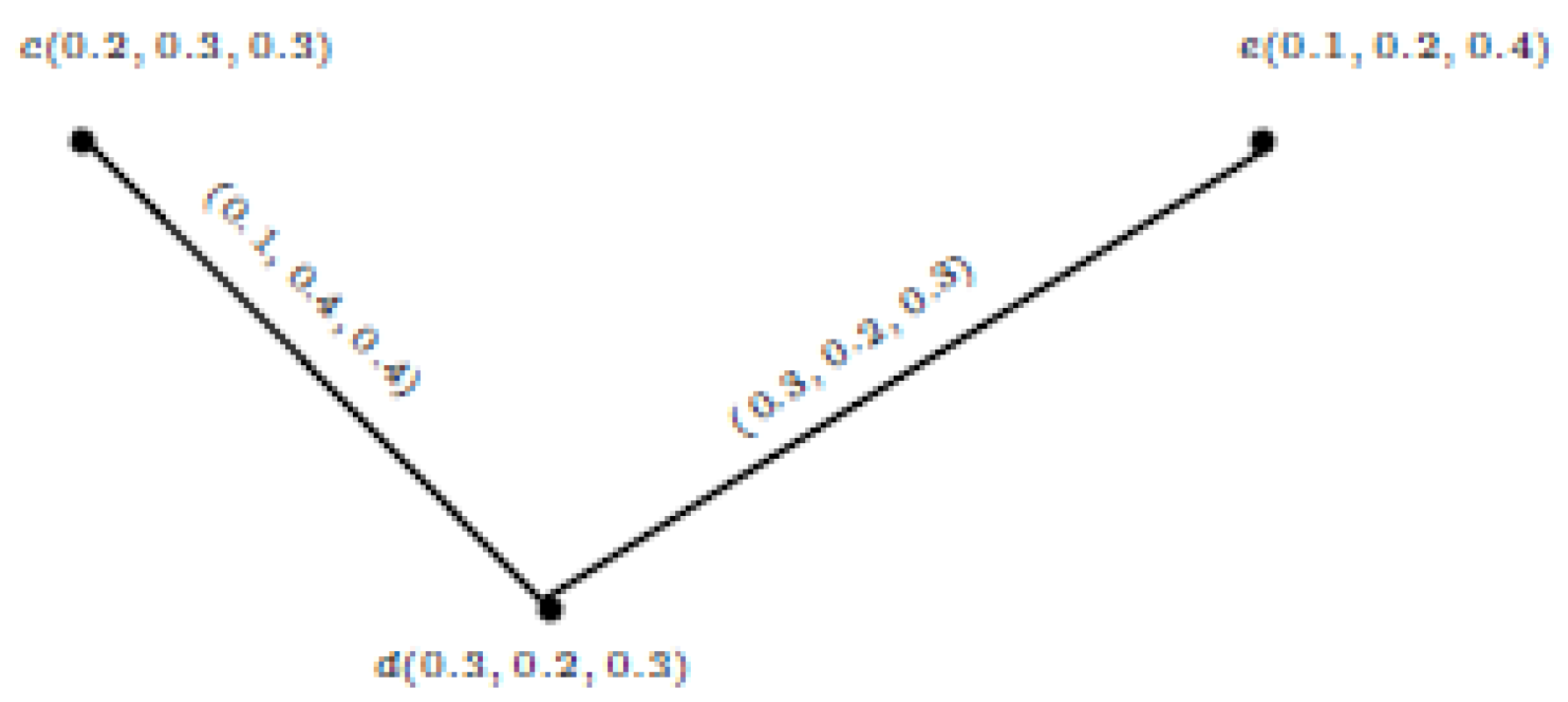
Example 10.

In Figure 16, ${\chi }_{U_1}\ge {\chi }_{W_2}$, ${\psi }_{U_1}\le {\psi }_{W_2}$, ${\chi }_{U_2}\ge {\chi }_{W_1}$, and ${\psi }_{U_2}\le {\psi }_{W_1}$. Then, the total degree of the vertex in SD is calculated by using the following formula:

$$\begin{array}{ccc}& & {\left(d_T\right)}_{G_1\oplus G_2}(m_1,m_2)=q{\left(d_T\right)}_{G_1}\left(m_1\right)+s{\left(d_T\right)}_{G_2}\left(m_2\right),\hfill \\ & & {\left(d_I\right)}_{G_1\oplus G_2}(m_1,m_2)=q{\left(d_I\right)}_{G_1}\left(m_1\right)+s{\left(d_I\right)}_{G_2}\left(m_2\right),\hfill \\ & & {\left(d_F\right)}_{G_1\oplus G_2}(m_1,m_2)=q{\left(d_F\right)}_{G_1}\left(m_1\right)+s{\left(d_F\right)}_{G_2}\left(m_2\right).\hfill \end{array}$$

$$\begin{array}{ccc}& & {\left(d_T\right)}_{G_1\oplus G_2}(a,c)=1·\left(0.2\right)+1·\left(0.2\right)=0.4,\hfill \\ & & {\left(d_I\right)}_{G_1\oplus G_2}(a,c)=1·\left(0.4\right)+1·\left(0.5\right)=0.9,\hfill \\ & & {\left(d_F\right)}_{G_1\oplus G_2}(a,c)=1·\left(0.4\right)+1·\left(0.5\right)=0.9,\hfill \\ & & {\left(d_T\right)}_{G_1\oplus G_2}(a,d)=1·\left(0.2\right)+1·\left(0.2\right)=0.4,\hfill \\ & & {\left(d_I\right)}_{G_1\oplus G_2}(a,d)=1·\left(0.4\right)+1·\left(0.5\right)=0.9,\hfill \\ & & {\left(d_F\right)}_{G_1\oplus G_2}(a,d)=1·\left(0.4\right)+1·\left(0.5\right)=0.9.\hfill \end{array}$$

Thus, ${\left(d\right)}_{G_1\oplus G_2}(a,c)=(0.4,0.9,0.9)$ and ${\left(d\right)}_{G_1\oplus G_2}(a,d)=(0.4,0.9,0.9)$.

Applying the same technique, we can obtain ${\left(d\right)}_{G_1\oplus G_2}(b,c)={\left(d\right)}_{G_1\oplus G_2}(b,d)=(0.4,0.9,0.9)$. Now, from direct calculations, we have:

$$\begin{array}{ccc}& & {\left(d_T\right)}_{G_1\oplus G_2}(a,c)=0.2+0.2=0.4,\hfill \\ & & {\left(d_I\right)}_{G_1\oplus G_2}(a,c)=0.4+0.5=0.9,\hfill \\ & & {\left(d_F\right)}_{G_1\oplus G_2}(a,c)=0.4+0.5=0.9,\hfill \\ & & {\left(d_T\right)}_{G_1\oplus G_2}(a,d)=0.2+0.2=0.4,\hfill \\ & & {\left(d_I\right)}_{G_1\oplus G_2}(a,d)=0.4+0.5=0.9,\hfill \\ & & {\left(d_F\right)}_{G_1\oplus G_2}(a,d)=0.4+0.5=0.9,\hfill \\ & & {\left(d_T\right)}_{G_1\oplus G_2}(b,c)=0.2+0.2=0.4,\hfill \\ & & {\left(d_I\right)}_{G_1\oplus G_2}(b,c)=0.4+0.5=0.9,\hfill \\ & & {\left(d_F\right)}_{G_1\oplus G_2}(b,c)=0.4+0.5=0.9,\hfill \\ & & {\left(d_T\right)}_{G_1\oplus G_2}(b,d)=0.2+0.2=0.4,\hfill \\ & & {\left(d_I\right)}_{G_1\oplus G_2}(b,d)=0.4+0.5=0.9,\hfill \\ & & {\left(d_F\right)}_{G_1\oplus G_2}(b,d)=0.4+0.5=0.9.\hfill \end{array}$$

From the calculated degree of nodes, we conclude that there is no difference in the answer when utilizing the formula or the direct technique.

Definition 13.

Let ${\mathbb{G}}_1=(U_1,W_1)$ and ${\mathbb{G}}_2=(U_2,W_2)$ be two PFGs. For any vertex $(u_1,u_2)\in$$V_1\times V_2$, we have:

$$\begin{array}{cc}\hfill {\left(t{d}_{\chi }\right)}_{{\mathbb{G}}_1⨁{\mathbb{G}}_2}(u_1,u_2)& =\sum _{(u_1,u_2)(w_1,w_2)\in E_1\times E_2.}({\chi }_{W_1}⨁{\chi }_{W_2})\left((u_1,u_2)(w_1,w_2)\right)+({\chi }_{U_1}⨁{\chi }_{U_2}(u_1,u_2)\hfill \\ \hfill & =\sum _{u_1=w_1,u_2{w}_2\in E_2}\wedge \{{\chi }_{U_1}\left(u_1\right),{\chi }_{W_2}\left(u_2{w}_2\right)\}\hfill \\ \hfill & +\sum _{u_1{w}_1\in E_1,u_2=w_2}\wedge \{{\chi }_{W_1}(u_1{w}_1,{\chi }_{U_2}\left(u_2\right)\}\hfill \\ \hfill & +\sum _{u_1{w}_1\notin E_{1}and{u}_2{w}_2\in E_2}\wedge \{{\chi }_{U_1}\left(u_1\right),{\chi }_{U_1}\left(w_1\right),{\chi }_{W_2}\left(u_2{w}_2\right)\}\hfill \\ \hfill & +\sum _{u_1{w}_1\in E_{1}and{u}_2{w}_2\notin E_2}\wedge \{{\chi }_{W_1}\left(u_1{w}_1\right),{\chi }_{U_2}\left(u_2\right),{\chi }_{U_2}\left(w_2\right)\}\hfill \\ \hfill & +\wedge \{{\chi }_{U_1}\left(u_1\right),{\chi }_{U_2}\left(u_2\right)\},\hfill \end{array}$$

$$\begin{array}{cc}\hfill {\left(t{d}_{\varphi }\right)}_{{\mathbb{G}}_1⨁{\mathbb{G}}_2}(u_1,u_2)& =\sum _{(u_1,u_2)(w_1,w_2)\in E_1\times E_2.}({\varphi }_{W_1}⨁{\varphi }_{W_2})\left((u_1,u_2)(w_1,w_2)\right)+({\varphi }_{U_1}⨁{\varphi }_{U_2}(u_1,u_2)\hfill \\ \hfill & =\sum _{u_1=w_1,u_2{w}_2\in E_2}\wedge \{{\varphi }_{U_1}\left(u_1\right),{\varphi }_{W_2}\left(u_2{w}_2\right)\}\hfill \\ \hfill & +\sum _{u_1{w}_1\in E_1,u_2=w_2}\wedge \{{\varphi }_{W_1}(u_1{w}_1,{\varphi }_{U_2}\left(u_2\right)\}\hfill \\ \hfill & +\sum _{u_1{w}_1\notin E_{1}and{u}_2{w}_2\in E_2}\wedge \{{\varphi }_{U_1}\left(u_1\right),{\varphi }_{U_1}\left(w_1\right),{\varphi }_{W_2}\left(u_2{w}_2\right)\}\hfill \\ \hfill & +\sum _{u_1{w}_1\in E_{1}and{u}_2{w}_2\notin E_2}\wedge \{{\varphi }_{W_1}\left(u_1{w}_1\right),{\varphi }_{U_2}\left(u_2\right),{\varphi }_{U_2}\left(w_2\right)\}\hfill \\ \hfill & +\wedge \{{\varphi }_{U_1}\left(u_1\right),{\varphi }_{U_2}\left(u_2\right)\},\hfill \end{array}$$

$$\begin{array}{cc}\hfill {\left(t{d}_{\psi }\right)}_{{\mathbb{G}}_1⨁{\mathbb{G}}_2}(u_1,u_2)& =\sum _{(u_1,u_2)(w_1,w_2)\in E_1\times E_2.}({\psi }_{W_1}⨁{\psi }_{W_2})\left((u_1,u_2)(w_1,w_2)\right)+({\psi }_{U_1}⨁{\psi }_{U_2}(u_1,u_2)\hfill \\ \hfill & =\sum _{u_1=w_1,u_2{w}_2\in E_2}\vee \{{\psi }_{U_1}\left(u_1\right),{\psi }_{W_2}\left(u_2{w}_2\right)\}\hfill \\ \hfill & +\sum _{u_1{w}_1\in E_1,u_2=w_2}\vee \{{\psi }_{W_1}(u_1{w}_1,{\psi }_{U_2}\left(u_2\right)\}\hfill \\ \hfill & +\sum _{u_1{w}_1\notin E_{1}and{u}_2{w}_2\in E_2}\vee \{{\psi }_{U_1}\left(u_1\right),{\psi }_{U_1}\left(w_1\right),{\psi }_{W_2}\left(u_2{w}_2\right)\}\hfill \\ \hfill & +\sum _{u_1{w}_1\in E_{1}and{u}_2{w}_2\notin E_2}\vee \{{\psi }_{W_1}\left(u_1{w}_1\right),{\psi }_{U_2}\left(u_2\right),{\psi }_{U_2}\left(w_2\right)\}\hfill \\ \hfill & +\vee \{{\psi }_{U_1}\left(u_1\right),{\psi }_{U_2}\left(u_2\right)\}.\hfill \end{array}$$

Theorem 5.

Suppose that ${\mathbb{G}}_1=(U_1,W_1)$ and ${\mathbb{G}}_2=(U_2,Y_2)$ are two PFGs. If

(i) ${\chi }_{U_1}\ge {\chi }_{W_2} and {\chi }_{U_2}\ge {\chi }_{W_1}$, then $\forall (u_1,u_2)\in V_1\times V_2$

$$\begin{array}{cc}\hfill {\left(t{d}_{\chi }\right)}_{{\mathbb{G}}_1⨁{\mathbb{G}}_2}(u_1,u_2)& =q{\left(t{d}_{\chi }\right)}_{{\mathbb{G}}_1}\left(u_1\right)+s{\left(t{d}_{\chi }\right)}_{{\mathbb{G}}_2}\left(u_2\right)\hfill \\ \hfill & -(q-1){\chi }_{{\mathbb{G}}_1}\left(u_1\right)-\vee \{{\chi }_{{\mathbb{G}}_1}\left(u_1\right),{\chi }_{{\mathbb{G}}_1}\left(u_1\right)\},\hfill \end{array}$$

(ii) ${\varphi }_{U_1}\le {\varphi }_{W_2} and {\varphi }_{U_2}\le {\varphi }_{W_1}$, then $\forall (u_1,u_2)\in V_1\times V_2$

$$\begin{array}{cc}\hfill {\left(t{d}_{\varphi }\right)}_{{\mathbb{G}}_1⨁{\mathbb{G}}_2}(u_1,u_2)& =q{\left(t{d}_{\varphi }\right)}_{{\mathbb{G}}_1}\left(u_1\right)+s{\left(t{d}_{\varphi }\right)}_{{\mathbb{G}}_2}\left(u_2\right)\hfill \\ \hfill & -(q-1){\varphi }_{{\mathbb{G}}_1}\left(u_1\right)-\vee \{{\varphi }_{{\mathbb{G}}_1}\left(u_1\right),{\varphi }_{{\mathbb{G}}_1}\left(u_1\right)\},\hfill \end{array}$$

(iii) ${\psi }_{U_1}\le {\psi }_{W_2} and {\psi }_{U_2}\ge {\psi }_{W_1}$, then $\forall (u_1,u_2)\in V_1\times V_2$

$$\begin{array}{cc}\hfill {\left(t{d}_{\psi }\right)}_{{\mathbb{G}}_1⨁{\mathbb{G}}_2}(u_1,u_2)& =q{\left(t{d}_{\psi }\right)}_{{\mathbb{G}}_1}\left(u_1\right)+s{\left(t{d}_{\psi }\right)}_{{\mathbb{G}}_2}\left(u_2\right)\hfill \\ \hfill & -(q-1){\psi }_{{\mathbb{G}}_1}\left(u_1\right)-\wedge \{{\psi }_{{\mathbb{G}}_1}\left(u_1\right),{\psi }_{{\mathbb{G}}_1}\left(u_1\right)\},\hfill \end{array}$$

$\forall (u_1,u_2)\in V_1\times V_2$, s = $\mid V_1\mid$$-{\left(d\right)}_{G_1}\left(u_1\right)$ and q = $\mid V_2\mid$$-{\left(d\right)}_{G_2}\left(u_2\right)$.

Proof. 

$\forall (u_1,u_2)\in V_1\times V_2$,

$$\begin{array}{cc}\hfill \left(t{d}_{\chi }\right)& {}_{{\mathbb{G}}_1⨁{\mathbb{G}}_2}(u_1,u_2)\hfill \\ \hfill & =\sum _{(u_1,u_2)(w_1,w_2)\in E_1\times E_2.}({\chi }_{W_1}⨁{\chi }_{W_2})\left((u_1,u_2)(w_1,w_2)\right)+({\chi }_{U_1}⨁{\chi }_{U_2})(u_1,u_2)\hfill \\ \hfill & =\sum _{u_1=w_1,u_2{w}_2\in E_2}\wedge \{{\chi }_{U_1}\left(u_1\right),{\chi }_{W_2}\left(u_2{w}_2\right)\}\hfill \\ \hfill & +\sum _{u_1{w}_1\in E_1,u_2=w_2}\wedge \{{\chi }_{W_1}\left(u_1{w}_1\right),{\chi }_{U_2}\left(u_2\right)\}\hfill \\ \hfill & +\sum _{u_1{w}_1\notin E_{1}and{u}_2{w}_2\in E_2}\wedge \{{\chi }_{U_1}\left(u_1\right),{\chi }_{U_1}\left(w_1\right),{\chi }_{W_2}\left(u_2{w}_2\right)\}\hfill \\ \hfill & +\sum _{u_1{w}_1\in E_{1}and{u}_2{w}_2\notin E_2}\wedge \{{\chi }_{W_1}\left(u_1{w}_1\right),{\chi }_{U_2}\left(u_2\right),{\chi }_{U_2}\left(w_2\right)\}\hfill \\ \hfill & +\vee \{{\chi }_{U_1}\left(u_1\right),{\chi }_{U_2}\left(u_2\right)\}\hfill \\ \hfill & =\sum _{u_2{w}_2\in E_2}{\chi }_{W_2}\left(u_2{w}_2\right)+\sum _{u_1{w}_1\in E_1}{\chi }_{W_1}\left(u_1{w}_1\right)\hfill \\ \hfill & +\sum _{u_1{w}_1\notin E_{1}and{u}_2{w}_2\in E_2}{\chi }_{W_2}\left(u_2{w}_2\right)+\sum _{u_1{w}_1\in E_{1}and{u}_2{w}_2\notin E_2}{\chi }_{W_1}\left(u_1{w}_1\right)\hfill \\ \hfill & +\vee \{{\chi }_{U_1}\left(u_1\right),{\chi }_{U_2}\left(u_2\right)\}\hfill \\ \hfill & =\sum _{u_2{w}_2\in E_2}{\chi }_{W_2}\left(u_2{w}_2\right)+\sum _{u_1{w}_1\in E_1}{\chi }_{W_1}\left(u_1{w}_1\right)+\sum _{u_1{w}_1\notin E_{1}and{u}_2{w}_2\in E_2}{\chi }_{W_2}\left(u_2{w}_2\right)\hfill \\ \hfill & +\sum _{u_1{w}_1\in E_{1}and{u}_2{w}_2\notin E_2}{\chi }_{W_1}\left(u_1{w}_1\right)+{\chi }_{U_1}\left(u_1\right)+{\chi }_{U_2}\left(u_2\right)-\vee \{{\chi }_{U_1}\left(u_1\right),{\chi }_{U_2}\left(u_2\right)\}\hfill \\ \hfill & =q{\left(t{d}_{\chi }\right)}_{{\mathbb{G}}_1}\left(u_1\right)+s{\left(t{d}_{\chi }\right)}_{{\mathbb{G}}_2}\left(u_2\right)\hfill \\ \hfill & -(q-1){\chi }_{{\mathbb{G}}_1}\left(u_1\right)-\vee \{{\chi }_{{\mathbb{G}}_1}\left(u_1\right),{\chi }_{{\mathbb{G}}_1}\left(u_1\right)\},\hfill \end{array}$$

$$\begin{array}{cc}\hfill \left(t{d}_{\varphi }\right)& {}_{{\mathbb{G}}_1⨁{\mathbb{G}}_2}(u_1,u_2)\hfill \\ \hfill & =\sum _{(u_1,u_2)(w_1,w_2)\in E_1\times E_2.}({\varphi }_{W_1}⨁{\varphi }_{W_2})\left((u_1,u_2)(w_1,w_2)\right)+({\varphi }_{U_1}⨁{\varphi }_{U_2})(u_1,u_2)\hfill \\ \hfill & =\sum _{u_1=w_1,u_2{w}_2\in E_2}\wedge \{{\varphi }_{U_1}\left(u_1\right),{\varphi }_{W_2}\left(u_2{w}_2\right)\}\hfill \\ \hfill & +\sum _{u_1{w}_1\in E_1,u_2=w_2}\wedge \{{\varphi }_{W_1}\left(u_1{w}_1\right),{\varphi }_{U_2}\left(u_2\right)\}\hfill \\ \hfill & +\sum _{u_1{w}_1\notin E_{1}and{u}_2{w}_2\in E_2}\wedge \{{\varphi }_{U_1}\left(u_1\right),{\varphi }_{U_1}\left(w_1\right),{\varphi }_{W_2}\left(u_2{w}_2\right)\}\hfill \\ \hfill & +\sum _{u_1{w}_1\in E_{1}and{u}_2{w}_2\notin E_2}\wedge \{{\varphi }_{W_1}\left(u_1{w}_1\right),{\varphi }_{U_2}\left(u_2\right),{\varphi }_{U_2}\left(w_2\right)\}\hfill \\ \hfill & +\wedge \{{\varphi }_{U_1}\left(u_1\right),{\varphi }_{U_2}\left(u_2\right)\hfill \\ \hfill & =\sum _{u_2{w}_2\in E_2}{\varphi }_{W_2}\left(u_2{w}_2\right)+\sum _{u_1{w}_1\in E_1}{\varphi }_{W_1}\left(u_1{w}_1\right)\hfill \\ \hfill & +\sum _{u_1{w}_1\notin E_{1}and{u}_2{w}_2\in E_2}{\varphi }_{W_2}\left(u_2{w}_2\right)\}+\sum _{u_1{w}_1\in E_{1}and{u}_2{w}_2\notin E_2}{\varphi }_{W_1}\left(u_1{w}_1\right)\hfill \\ \hfill & +\wedge \{{\varphi }_{U_1}\left(u_1\right),{\varphi }_{U_2}\left(u_2\right)\}\hfill \\ \hfill & =\sum _{u_2{w}_2\in E_2}{\varphi }_{W_2}\left(u_2{w}_2\right)+\sum _{u_1{w}_1\in E_1}{\varphi }_{W_1}\left(u_1{w}_1\right)+\sum _{u_1{w}_1\notin E_{1}and{u}_2{w}_2\in E_2}{\varphi }_{W_2}\left(u_2{w}_2\right)\hfill \\ \hfill & +\sum _{u_1{w}_1\in E_{1}and{u}_2{w}_2\notin E_2}{\varphi }_{W_1}\left(u_1{w}_1\right)+{\varphi }_{U_1}\left(u_1\right)+{\varphi }_{U_2}\left(u_2\right)-\vee \{{\varphi }_{U_1}\left(u_1\right),{\varphi }_{U_2}\left(u_2\right)\}\hfill \\ \hfill & =q{\left(t{d}_{\varphi }\right)}_{{\mathbb{G}}_1}\left(u_1\right)+s{\left(t{d}_{\varphi }\right)}_{{\mathbb{G}}_2}\left(u_2\right)\hfill \\ \hfill & -(q-1){\varphi }_{{\mathbb{G}}_1}\left(u_1\right)-\vee \{{\varphi }_{{\mathbb{G}}_1}\left(u_1\right),{\varphi }_{{\mathbb{G}}_1}\left(u_1\right)\},\hfill \end{array}$$

$$\begin{array}{cc}\hfill \left(t{d}_{\psi }\right)& {}_{{\mathbb{G}}_1⨁{\mathbb{G}}_2}(u_1,u_2)\hfill \\ \hfill & =\sum _{(u_1,u_2)(w_1,w_2)\in E_1\times E_2.}({\psi }_{W_1}⨁{\psi }_{W_2})\left((u_1,u_2)(w_1,w_2)\right)+({\psi }_{U_1}⨁{\psi }_{U_2})(u_1,u_2)\hfill \\ \hfill & =\sum _{u_1=w_1,u_2{w}_2\in E_2}\vee \{{\psi }_{U_1}\left(u_1\right),{\psi }_{W_2}\left(u_2{w}_2\right)\}\hfill \\ \hfill & +\sum _{u_1{w}_1\in E_1,u_2=w_2}\vee \{{\psi }_{W_1}\left(u_1{w}_1\right),{\psi }_{U_2}\left(u_2\right)\}\hfill \\ \hfill & +\sum _{u_1{w}_1\notin E_{1}and{u}_2{w}_2\in E_2}\vee \{{\psi }_{U_1}\left(u_1\right),{\psi }_{U_1}\left(w_1\right),{\psi }_{W_2}\left(u_2{w}_2\right)\hfill \\ \hfill & +\sum _{u_1{w}_1\in E_{1}and{u}_2{w}_2\notin E_2}\vee \{{\psi }_{W_1}\left(u_1{w}_1\right),{\psi }_{U_2}\left(u_2\right),{\psi }_{U_2}\left(w_2\right)\}\hfill \\ \hfill & +\wedge \{{\psi }_{U_1}\left(u_1\right),{\psi }_{U_2}\left(u_2\right)\}\hfill \\ \hfill & =\sum _{u_2{w}_2\in E_2}{\psi }_{W_2}\left(u_2{w}_2\right)+\sum _{u_1{w}_1\in E_1}{\psi }_{W_1}\left(u_1{w}_1\right)\hfill \\ \hfill & +\sum _{u_1{w}_1\notin E_{1}and{u}_2{w}_2\in E_2}{\psi }_{W_2}\left(u_2{w}_2\right)\}+\sum _{u_1{w}_1\in E_{1}and{u}_2{w}_2\notin E_2}{\psi }_{W_1}\left(u_1{w}_1\right)\hfill \\ \hfill & +\wedge \{{\psi }_{U_1}\left(u_1\right),{\psi }_{U_2}\left(u_2\right)\}\hfill \\ \hfill & =\sum _{u_2{w}_2\in E_2}{\psi }_{W_2}\left(u_2{w}_2\right)+\sum _{u_1{w}_1\in E_1}{\psi }_{W_1}\left(u_1{w}_1\right)+\sum _{u_1{w}_1\notin E_{1}and{u}_2{w}_2\in E_2}{\psi }_{W_2}\left(u_2{w}_2\right)\}\hfill \\ \hfill & +\sum _{u_1{w}_1\in E_{1}and{u}_2{w}_2\notin E_2}{\psi }_{W_1}\left(u_1{w}_1\right)+{\psi }_{U_1}\left(u_1\right)+{\psi }_{U_2}\left(u_2\right)-\wedge \{{\psi }_{U_1}\left(u_1\right),{\psi }_{U_2}\left(u_2\right)\}\hfill \\ \hfill & =q{\left(t{d}_{\psi }\right)}_{{\mathbb{G}}_1}\left(u_1\right)+s{\left(t{d}_{\psi }\right)}_{{\mathbb{G}}_2}\left(u_2\right)\hfill \\ \hfill & -(q-1){\psi }_{{\mathbb{G}}_1}\left(u_1\right)-\wedge \{{\psi }_{{\mathbb{G}}_1}\left(u_1\right),{\psi }_{{\mathbb{G}}_1}\left(u_1\right)\},\hfill \end{array}$$

where the values of s and q are as follows: s = $\mid V_1\mid$−${\left(d\right)}_{G_1}\left(u_1\right)$ and q = $\mid V_2\mid$−${\left(d\right)}_{G_2}\left(u_2\right)$ □

Example 11.

We find the total degree of nodes by using Example 9.

$$\begin{array}{c}\hfill {\left(d_{\chi }\right)}_{{\mathbb{G}}_1⨁{\mathbb{G}}_2}(a,e)=q{\left(d_{\chi }\right)}_{{\mathbb{G}}_1}\left(a\right)+s{\left(d_{\chi }\right)}_{{\mathbb{G}}_2}\left(e\right)\end{array}$$

$$\begin{array}{cc}\hfill s& =\mid V_1\mid -{\left(d\right)}_{G_1}\left(a\right)\hfill \\ \hfill & =2-1=1\hfill \end{array}$$

Now,

$$\begin{array}{cc}\hfill q& =\mid V_2\mid -{\left(d\right)}_{G_2}\left(e\right)\hfill \\ \hfill & =4-2=2\hfill \end{array}$$

$$\begin{array}{cc}\hfill {\left(t{d}_{\chi }\right)}_{{\mathbb{G}}_1⨁{\mathbb{G}}_2}(a,e)& =q{\left(t{d}_{\chi }\right)}_{{\mathbb{G}}_1}\left(a\right)+s{\left(t{d}_{\chi }\right)}_{{\mathbb{G}}_2}\left(e\right)\hfill \\ \hfill & -(s-1){\chi }_{{\mathbb{G}}_2}\left(e\right)-(q-1){\chi }_{{\mathbb{G}}_1}\left(a\right)-\vee \{{\chi }_{{\mathbb{G}}_1}\left(a\right),{\chi }_{{\mathbb{G}}_2}\left(e\right)\}\hfill \\ \hfill & =2(0.2+0.2)+1(0.3+0.3+0.2)-(1-1)\left(0.3\right)-(2-1)\left(0.2\right)-\vee \{0.2,0.3\}\hfill \\ \hfill & =2\left(0.4\right)+0.8-0.2-0.3=1.1,\hfill \end{array}$$

$$\begin{array}{c}\hfill {\left(t{d}_{\varphi }\right)}_{{\mathbb{G}}_1⨁{\mathbb{G}}_2}(a,e)=1.6,\end{array}$$

$$\begin{array}{cc}\hfill {\left(t{d}_{\psi }\right)}_{{\mathbb{G}}_1⨁{\mathbb{G}}_2}(a,e)& =0.6,\hfill \end{array}$$

$$\begin{array}{c}\hfill {\left(td\right)}_{{\mathbb{G}}_1⨁{\mathbb{G}}_2}(a,e)=(1.1,1.6,0.6).\end{array}$$

We conclude from the calculations that the total degrees of nodes calculated by the formula of the above theorem and by the direct method are equal.

Definition 14.

The RP ${\mathbb{G}}_1•{\mathbb{G}}_2=(U_1•U_2,W_1•W_2)$ of two PFGs ${\mathbb{G}}_1=(U_1,W_1)$ and ${\mathbb{G}}_2=(U_2,W_2)$ is defined as:

(i)

$$\begin{array}{c}\hfill ({\chi }_{U_1}•{\chi }_{U_2})(u_1,u_2)=\vee \{{\chi }_{U_1}\left(u_1\right),{\chi }_{U_2}\left(u_2\right)\},\end{array}$$

$$\begin{array}{c}\hfill ({\varphi }_{U_1}•{\varphi }_{U_2})(u_1,u_2)=\vee \{{\varphi }_{U_1}\left(u_1\right),{\varphi }_{U_2}\left(u_2\right)\},\end{array}$$

$$\begin{array}{c}\hfill ({\psi }_{U_1}•{\psi }_{U_2})(u_1,u_2)=\wedge \{{\psi }_{U_1}\left(u_1\right),{\psi }_{U_2}\left(u_2\right)\},\end{array}$$

$\forall (u_1,u_2)\in (V_1\times V_2)$.

(ii)

$$\begin{array}{c}\hfill ({\chi }_{W_1}•{\chi }_{W_2})\left((u_1,u_2)(w_1,w_2)\right)={\chi }_{W_1}\left(u_1{w}_1\right),\end{array}$$

$$\begin{array}{c}\hfill ({\varphi }_{W_1}•{\varphi }_{W_2})\left((u_1,u_2)(w_1,w_2)\right)={\varphi }_{W_1}\left(u_1{w}_1\right),\end{array}$$

$$\begin{array}{c}\hfill ({\psi }_{W_1}•{\psi }_{W_2})\left((u_1,u_2)(w_1,w_2)\right)={\psi }_{W_1}\left(u_1{w}_1\right),\end{array}$$

$\forall u_1{w}_1\in E_1,u_2\ne w_2$.

Example 12.

Taking two PFGs ${\mathbb{G}}_1$ and ${\mathbb{G}}_2$, as in Figure 17 and Figure 18, we can see the RP of two PFGs ${\mathbb{G}}_1$ and ${\mathbb{G}}_2$, that is, ${\mathbb{G}}_1•{\mathbb{G}}_2$, in Figure 19.

For node $(b,e)$, we find Mv, IDv, and NMv as follows:

$$\begin{array}{ccc}& & ({\chi }_{U_1}•{\chi }_{U_2})(b,e)=\vee \{{\chi }_{U_1}\left(b\right),{\chi }_{U_2}\left(e\right)\}\hfill \\ & & =\vee \{0.2,0.1\}=0.2,\hfill \\ & & ({\varphi }_{U_1}•{\varphi }_{U_2})(b,e)=\wedge \{{\varphi }_{U_1}\left(b\right),{\varphi }_{U_2}\left(e\right)\}\hfill \\ & & =\wedge \{0.4,0.2\}=0.2,\hfill \\ & & ({\psi }_{U_1}•{\psi }_{U_2})(b,e)=\wedge \{{\psi }_{U_1}\left(b\right),{\psi }_{U_2}\left(e\right)\}\hfill \\ & & =\wedge \{0.4,0.4\}=0.4\hfill \end{array}$$

for $b\in V_1$ and $e\in V_2$.

For arc $(a,c)(b,d)$, we find Mv, IDv, and NMv.

$$\begin{array}{ccc}& & ({\chi }_{W_1}•{\chi }_{W_2})\left((a,c)(b,d)\right)={\chi }_{W_1}\left(ab\right)=0.1,\hfill \\ & & ({\psi }_{W_1}•{\psi }_{W_2})\left((a,c)(b,d)\right)={\psi }_{W_1}\left(ab\right)=0.5,\hfill \\ & & ({\psi }_{W_1}•{\psi }_{W_2})\left((a,c)(b,d)\right)={\psi }_{W_1}\left(ab\right)=0.4\hfill \end{array}$$

for $ab\in E_1$ and $c\ne d$.

Hence, we can calculate Mv, IDv, and NMv for other nodes and arcs.

Proposition 4.

The RP of two PFGs ${\mathbb{G}}_1$ and ${\mathbb{G}}_2$ is a PFG.

Proof. 

Suppose that ${\mathbb{G}}_1=(U_1,W_1)$ and ${\mathbb{G}}_2=(U_2,W_2)$ are two PFGs on crisp graphs $G_1=(V_1,E_1)$ and $G_2=(V_2,E_2)$, respectively, and $\left((u_1,u_2)(w_1,w_2)\right)\in E_1\times E_2$. If $u_1{w}_1\in E_{1}and{u}_2\ne w_2$, then we have:

$$\begin{array}{cc}\hfill ({\chi }_{W_1}•{\chi }_{W_2})\left((u_1,u_2)(w_1,w_2)\right)& ={\chi }_{W_1}\left(u_1{w}_1\right)\hfill \\ \hfill & \le \wedge \{{\chi }_{U_1}\left(u_1\right),{\chi }_{U_1}\left(w_1\right)\}\hfill \\ \hfill & \le \vee \{\wedge \{{\chi }_{U_1}\left(u_1\right),{\chi }_{U_1}\left(w_1\right)\},\wedge \{{\chi }_{U_2}\left(u_2\right),{\chi }_{U_2}\left(w_2\right)\}\}\hfill \\ \hfill & =\wedge \{\vee \{{\chi }_{U_1}\left(u_1\right),{\chi }_{U_1}\left(w_1\right)\},\vee \{{\chi }_{U_2}\left(u_2\right),{\chi }_{U_2}\left(w_2\right)\}\}\hfill \\ \hfill & =\wedge \{({\chi }_{U_1}•{\chi }_{U_2})(u_1,u_2),({\chi }_{U_1}•{\chi }_{U_2})(w_1,w_2)\},\hfill \end{array}$$

$$\begin{array}{cc}\hfill ({\varphi }_{W_1}•{\varphi }_{W_2})\left((u_1,u_2)(w_1,w_2)\right)& ={\varphi }_{W_1}\left(u_1{w}_1\right)\hfill \\ \hfill & \ge \wedge \{{\varphi }_{U_1}\left(u_1\right),{\varphi }_{U_1}\left(w_1\right)\}\hfill \\ \hfill & \ge \vee \{\wedge \{{\varphi }_{U_1}\left(u_1\right),{\varphi }_{U_1}\left(w_1\right)\},\wedge \{{\varphi }_{U_2}\left(u_2\right),{\varphi }_{U_2}\left(w_2\right)\}\}\hfill \\ \hfill & =\wedge \{\vee \{{\varphi }_{U_1}\left(u_1\right),{\varphi }_{U_1}\left(w_1\right)\},\vee \{{\varphi }_{U_2}\left(u_2\right),{\varphi }_{U_2}\left(w_2\right)\}\}\hfill \\ \hfill & =\wedge \{({\varphi }_{U_1}•{\varphi }_{U_2})(u_1,u_2),({\varphi }_{U_1}•{\varphi }_{U_2})(w_1,w_2)\},\hfill \end{array}$$

$$\begin{array}{cc}\hfill ({\psi }_{W_1}•{\psi }_{W_2})\left((u_1,u_2)(w_1,w_2)\right)& ={\psi }_{W_1}\left(u_1{w}_1\right)\hfill \\ \hfill & \ge \vee \{{\psi }_{U_1}\left(u_1\right),{\psi }_{U_1}\left(w_1\right)\}\hfill \\ \hfill & \ge \wedge \{\vee \{{\psi }_{U_1}\left(u_1\right),{\psi }_{U_1}\left(w_1\right)\},\vee \{{\psi }_{U_2}\left(u_2\right),{\psi }_{U_2}\left(w_2\right)\}\}\hfill \\ \hfill & =\vee \{\wedge \{{\psi }_{U_1}\left(u_1\right),{\psi }_{U_1}\left(w_1\right)\},\wedge \{{\psi }_{U_2}\left(u_2\right),{\psi }_{U_2}\left(w_2\right)\}\}\hfill \\ \hfill & =\vee \{({\psi }_{U_1}•{\psi }_{U_2})(u_1,u_2),({\psi }_{U_1}•{\psi }_{U_2})(w_1,w_2)\}.\hfill \end{array}$$

□

Definition 15.

Suppose that ${\mathbb{G}}_1=(U_1,W_1)$ and ${\mathbb{G}}_2=(U_2,W_2)$ are two PFGs. For any node $(u_1,u_2)\in V_1\times V_2$, we have:

$$\begin{array}{cc}\hfill {\left(d_{\chi }\right)}_{{\mathbb{G}}_1•{\mathbb{G}}_2}(u_1,u_2)& =\sum _{(u_1,u_2)(w_1,w_2)\in E_1\times E_2.}({\chi }_{W_1}•{\chi }_{W_2})\left((u_1,u_2)(w_1,w_2)\right)\hfill \\ \hfill & =\sum _{u_1{w}_1\in E_1,u_2\ne w_2}{\chi }_{W_1}\left(u_1{w}_1\right)\hfill \\ \hfill & ={\left(d_{\chi }\right)}_{{\mathbb{G}}_1}\left(u_1\right),\hfill \end{array}$$

$$\begin{array}{cc}\hfill {\left(d_{\varphi }\right)}_{{\mathbb{G}}_1•{\mathbb{G}}_2}(u_1,u_2)& =\sum _{(u_1,u_2)(w_1,w_2)\in E_1\times E_2.}({\varphi }_{W_1}•{\varphi }_{W_2})\left((u_1,u_2)(w_1,w_2)\right)\hfill \\ \hfill & =\sum _{u_1{w}_1\in E_1,u_2\ne w_2}{\varphi }_{W_1}\left(u_1{w}_1\right)\hfill \\ \hfill & ={\left(d_{\varphi }\right)}_{{\mathbb{G}}_1}\left(u_1\right),\hfill \end{array}$$

$$\begin{array}{cc}\hfill {\left(d_{\psi }\right)}_{{\mathbb{G}}_1•{\mathbb{G}}_2}(u_1,u_2)& =\sum _{(u_1,u_2)(w_1,w_2)\in E_1\times E_2.}({\psi }_{W_1}•{\psi }_{W_2})\left((u_1,u_2)(w_1,w_2)\right)\hfill \\ \hfill & =\sum _{u_1{w}_1\in E_1,u_2\ne w_2}{\psi }_{W_1}\left(u_1{w}_1\right)\hfill \\ \hfill & ={\left(d_{\psi }\right)}_{{\mathbb{G}}_1}\left(u_1\right).\hfill \end{array}$$

Definition 16.

Suppose that ${\mathbb{G}}_1=(U_1,W_1)$ and ${\mathbb{G}}_2=(U_2,W_2)$ are two PFGs. For any node $(u_1,u_2)\in V_1\times V_2$, we have:

$$\begin{array}{cc}\hfill {\left(t{d}_{\chi }\right)}_{{\mathbb{G}}_1•{\mathbb{G}}_2}(u_1,u_2)& =\sum _{(u_1,u_2)(w_1,w_2)\in E_1\times E_2.}({\chi }_{W_1}•{\chi }_{W_2})\left((u_1,u_2)(w_1,w_2)\right)+({\chi }_{U_1}•{\chi }_{U_2})(u_1,u_2)\hfill \\ \hfill & =\sum _{u_1{w}_1\in E_1,u_2\ne w_2}{\chi }_{W_1}\left(u_1{w}_1\right)+\wedge \{{\chi }_{U_1}\left(u_1\right),{\chi }_{U_2}\left(u_2\right)\}\hfill \\ \hfill & =\sum _{u_1{w}_1\in E_1,u_2\ne w_2}{\chi }_{W_1}\left(u_1{w}_1\right)+{\chi }_{U_1}\left(u_1\right)+{\chi }_{U_2}\left(u_2\right)-\vee \{{\chi }_{U_1}\left(u_1\right),{\chi }_{U_2}\left(u_2\right)\}\hfill \\ \hfill & ={\left(t{d}_{\chi }\right)}_{{\mathbb{G}}_1}\left(u_1\right)+{\chi }_{U_2}\left(u_2\right)-\vee \{{\chi }_{U_1}\left(u_1\right),{\chi }_{U_2}\left(u_2\right)\},\hfill \end{array}$$

$$\begin{array}{cc}\hfill {\left(t{d}_{\varphi }\right)}_{{\mathbb{G}}_1•{\mathbb{G}}_2}(u_1,u_2)& =\sum _{(u_1,u_2)(w_1,w_2)\in E_1\times E_2.}({\varphi }_{W_1}•{\varphi }_{W_2})\left((u_1,u_2)(w_1,w_2)\right)+({\varphi }_{U_1}•{\varphi }_{U_2}(u_1,u_2))\hfill \\ \hfill & =\sum _{u_1{w}_1\in E_1,u_2\ne w_2}{\varphi }_{W_1}\left(u_1{w}_1\right)+\wedge \{{\varphi }_{U_1}\left(u_1\right),{\varphi }_{U_2}\left(u_2\right)\}\hfill \\ \hfill & =\sum _{u_1{w}_1\in E_1,u_2\ne w_2}{\varphi }_{W_1}\left(u_1{w}_1\right)+{\varphi }_{U_1}\left(u_1\right)+{\varphi }_{U_2}\left(u_2\right)-\vee \{{\varphi }_{U_1}\left(u_1\right),{\varphi }_{U_2}\left(u_2\right)\}\hfill \\ \hfill & ={\left(t{d}_{\varphi }\right)}_{{\mathbb{G}}_1}\left(u_1\right)+{\varphi }_{U_2}\left(u_2\right)-\vee \{{\varphi }_{U_1}\left(u_1\right),{\varphi }_{U_2}\left(u_2\right)\},\hfill \end{array}$$

$$\begin{array}{cc}\hfill {\left(t{d}_{\psi }\right)}_{{\mathbb{G}}_1•{\mathbb{G}}_2}(u_1,u_2)& =\sum _{(u_1,u_2)(w_1,w_2)\in E_1\times E_2.}({\psi }_{W_1}•{\psi }_{W_2})\left((u_1,u_2)(w_1,w_2)\right)+({\psi }_{U_1}•{\psi }_{U_2}(u_1,u_2))\hfill \\ \hfill & =\sum _{u_1{w}_1\in E_1,u_2\ne w_2}{\psi }_{W_1}\left(u_1{w}_1\right)+\vee \{{\psi }_{U_1}\left(u_1\right),{\psi }_{U_2}\left(u_2\right)\}\hfill \\ \hfill & =\sum _{u_1{w}_1\in E_1,u_2\ne w_2}{\psi }_{W_1}\left(u_1{w}_1\right)+{\psi }_{U_1}\left(u_1\right)+{\psi }_{U_2}\left(u_2\right)-\wedge \{{\psi }_{U_1}\left(u_1\right),{\psi }_{U_2}\left(u_2\right)\}\hfill \\ \hfill & ={\left(t{d}_{\psi }\right)}_{{\mathbb{G}}_1}\left(u_1\right)+{\psi }_{U_2}\left(u_2\right)-\wedge \{{\psi }_{U_1}\left(u_1\right),{\psi }_{U_2}\left(u_2\right)\}.\hfill \end{array}$$

Example 13.

We calculate the degree and the total degree of node $(b,e)$ by using Example 12.

$$\begin{array}{cc}\hfill {\left(d_{\chi }\right)}_{{\mathbb{G}}_1•{\mathbb{G}}_2}(b,e)& ={\left(d_{\chi }\right)}_{{\mathbb{G}}_1}\left(b\right)\hfill \\ \hfill & =0.1,\hfill \end{array}$$

$$\begin{array}{cc}\hfill {\left(d_{\varphi }\right)}_{{\mathbb{G}}_1•{\mathbb{G}}_2}(b,e)& ={\left(d_{\varphi }\right)}_{{\mathbb{G}}_1}\left(b\right)\hfill \\ \hfill & =0.5,\hfill \end{array}$$

$$\begin{array}{cc}\hfill {\left(d_{\psi }\right)}_{{\mathbb{G}}_1•{\mathbb{G}}_2}(b,e)& ={\left(d_{\psi }\right)}_{{\mathbb{G}}_1}\left(b\right)\hfill \\ \hfill & =0.4.\hfill \end{array}$$

Therefore,

$$\begin{array}{cc}\hfill {\left(d\right)}_{{\mathbb{G}}_1•{\mathbb{G}}_2}(b,e)& =(0.1,0.5,0.4)\hfill \end{array}$$

Additionally, the total degree of vertex (a,e) can be determined as follows:

$$\begin{array}{cc}\hfill & {\left(t{d}_{\chi }\right)}_{{\mathbb{G}}_1•{\mathbb{G}}_2}(a,e)\hfill \\ \hfill & ={\left(t{d}_{\chi }\right)}_{{\mathbb{G}}_1}\left(a\right)+{\chi }_{U_2}\left(e\right)-\vee \{{\chi }_{U_1}\left(a\right),{\chi }_{U_2}\left(e\right)\}\hfill \\ \hfill & =(0.2+0.1)+0.1-\vee (0.2,0.1)\hfill \\ \hfill & =0.2,\hfill \end{array}$$

$$\begin{array}{cc}\hfill & {\left(t{d}_{\varphi }\right)}_{{\mathbb{G}}_1•{\mathbb{G}}_2}(a,e)\hfill \\ \hfill & ={\left(t{d}_{\varphi }\right)}_{{\mathbb{G}}_1}\left(a\right)+{\varphi }_{U_2}\left(e\right)-\wedge \{{\varphi }_{U_1}\left(a\right),{\varphi }_{U_2}\left(e\right)\}\hfill \\ \hfill & =(0.4+0.5)+0.2-\wedge (0.4,0.2)\hfill \\ \hfill & =0.9,\hfill \end{array}$$

$$\begin{array}{cc}\hfill & {\left(t{d}_{\psi }\right)}_{{\mathbb{G}}_1•{\mathbb{G}}_2}(a,e)\hfill \\ \hfill & ={\left(t{d}_{\psi }\right)}_{{\mathbb{G}}_1}\left(a\right)+{\psi }_{U_2}\left(e\right)-\wedge \{{\psi }_{U_1}\left(a\right),{\psi }_{U_2}\left(e\right)\}\hfill \\ \hfill & =(0.4+0.4)+0.4-\wedge (0.4,0.4)\hfill \\ \hfill & =0.8.\hfill \end{array}$$

Thus,

$$\begin{array}{c}\hfill {\left(td\right)}_{{\mathbb{G}}_1•{\mathbb{G}}_2}(a,e)=(0.2,0.9,0.8)\end{array}$$

We can calculate these for all other nodes.

4. Application of PFG in Networking

Definition 17

([23]). Let X, Y ∈ R be a universal set; then,

$$\begin{array}{c}\hfill R=\{((x,y),{\chi }_R(x,y),{\varphi }_R(x,y),{\psi }_R(x,y)):(x,y)\in X\times Y\}\end{array}$$

is called a picture fuzzy relation from X to Y, where

$$\begin{array}{c}\hfill {\chi }_R(x,y):X\times Y,\end{array}$$

$$\begin{array}{c}\hfill {\varphi }_R(x,y):X\times Y,\end{array}$$

$$\begin{array}{c}\hfill {\psi }_R(x,y):X\times Y\end{array}$$

satisfy the condition $0\le {\chi }_R(x,y)+{\varphi }_R(x,y)+{\psi }_R(x,y)\le 1$ for every (x,y) ∈ X × Y.

A picture fuzzy relation (PFR) is called a directed picture fuzzy relation (directed PFR) if the ties are oriented from one vertex to another vertex.

Marketing comprises the activities and processes for creating, delivering, communicating, and exchanging offerings that are important to clients and partners. Digital marketing is a component of marketing that uses the internet and online-based digital technologies, such as mobile phones, desktop computers, and other digital media and platforms, to promote products and services. The popularity of social networks such as Google, YouTube, Facebook, Twitter, WhatsApp, and Research Gate is growing daily. They have widely used business platforms. In social networks, we commonly exchange many types of information and problems. These exchanges facilitate online business (e-commerce and e-business), political campaigns, future developments, and customer interaction. Digital marketing plays an important role in raising public awareness by rapidly communicating information about natural disasters and terrorist/criminal attacks to a crowd. The development of digital marketing is effectively a result of technology development. The first key event happened in 1971 when Ray Tomlison sent the first email, and his technology continues to help people to send or receive files through different machines. Digital marketing is online marketing. A social network is a collection of vertices and edges. The vertices are used to represent cities, groups, countries, institutions, places, etc., and edges are used to describe the relationships between vertices. A social network is represented by a classical graph, in which actors are represented by vertices and connections between nodes are represented by edges. Fuzzy graphs, on the other hand, can correctly model social networks. Since all nodes in a classical graph have the same importance, all social units in history’s social networks are equally represented. Moreover, in actuality, not all social units are of equal importance. In other words, in a classical graph, all edges have the same strength. In all existing social networks, the strength of the relationship between two social units is assumed to be the same, but this may be false in real life.

In a picture fuzzy social network (PFSN), an account of an individual or company, i.e., a social unit, is defined by nodes, and if two social units have a relationship, they are joined by a single arrow. In reality, each vertex, i.e., a social unit, engages in some negative, neutral, and positive activities. The bad, neutral, and good membership values of the vertices are used to demonstrate the bad, neutral, and satisfactory initiatives, and the bad, neutral, and good membership degrees of the edges can be used to describe the strength of the relationship between two vertices. For example, three people have an extensive understanding of educational activities and teaching methods. We can describe these three types of vertex and edge membership degrees using PFS, which has three membership values for each element. This form of social network is a functional example of a PFG. The centrality of a vertex is more central than that of another vertex. A central person is closer than another person and can convey or access more information. The diameter of a social network is defined as the largest distance between two vertices in the network.

Let $G_{mn}^{\prime }$ = $(V,E_{mi}^{\prime })$ represent an undirected PFG. We can define an undirected PFSN as a picture fuzzy relational structure $G_{mi}^{\prime }$ = $(V,E_{mi}^{\prime })$, where $V=\{v_1,v_2,...,v_i\}$ denotes non-empty picture fuzzy vertices, and $E_{mi}^{\prime }$=$\left(\begin{array}{ccccc}{e}_{11}^{\prime }& .& .& .& e_{1i}^{\prime }\\ .& .& & & .\\ .& & .& & .\\ .& & & .& .\\ e_{i1}^{\prime }& .& .& .& e_{ii}^{\prime }\end{array}\right)$ denotes an undirected picture fuzzy relation on V. An example of an undirected PFSN is shown in Figure 20. For an undirected PFSN, arcs are simply an absent or present undirected PFR, with no other information attached.

Let $G_{hi}^{\prime }$ = $(V,E_{hi}^{\prime })$ represent a directed PFG. We can describe a directed PFSN as a PFRal structure $G_{hi}^{\prime }$ = $(V,E_{hi}^{\prime })$, where $V=\{v_1,v_2,...,v_i\}$ denotes non-empty picture fuzzy vertices, and $E_{mn}^{\prime }$ = $\left(\begin{array}{ccccc}{e}_{11}^{\prime }& .& .& .& e_{1i}^{\prime }\\ .& .& & & .\\ .& & .& & .\\ .& & & .& .\\ e_{i1}^{\prime }& .& .& .& e_{ii}^{\prime }\end{array}\right)$ represents an undirected PFR on V.

The directed PFR is considered in a directed PFSN. A directed PFG is more efficient for modeling the social network because arcs that are considered with a directed PFR contain more information. The values of $e_{jk}^{\prime }$ and $e_{kj}^{\prime }$ are equal in an undirected PFSN. However, $e_{jk}^{\prime }$ and $e_{kj}^{\prime }$ are not equal in a directed PFSN.

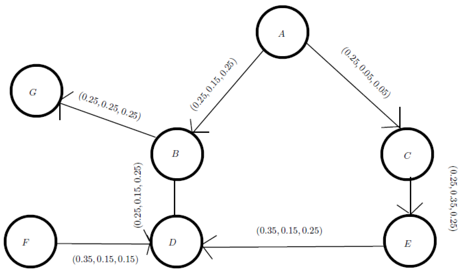
A small example of a directed PFSN is shown in Figure 21. Let $G_{hi}^{\prime }$ =$(V,E_{hi}^{\prime })$ be a directed PFSN, and PFS is used to describe the arc lengths of $G_{hi}^{\prime }$. The sum of the lengths of the arcs that are adjacent to social vertex $v_j$ is called the picture fuzzy in-degree centrality (PFIDC) of node $v_j$. The PFIDC of node $v_j$,$d_I^{\prime }\left(vi\right)$ is described as:

$$\begin{array}{cc}\hfill d_I^{\prime }\left(v_j\right)& =\sum _{k=1,...n,k\ne j}{e}_{kj}^{\prime }\hfill \end{array}$$

The sum of the lengths of the arcs that are adjacent to social vertex $v_j$ is called the picture fuzzy out-degree centrality (PFODC) of node $v_j$. The PFODC of node $v_j$,$d_I^{\prime }\left(vi\right)$ is described as:

$$\begin{array}{cc}\hfill d_o^{\prime }\left(v_j\right)& =\sum _{k=1,...n,k\ne j}{e}_{kj}^{\prime }\hfill \end{array}$$

The symbol ∑ represents the addition operation of PFS. $e_{kj}^{\prime }$ is a PFS associated with arc (j,k). The sum of PFIDC and PFODC of vertex $v_j$ is called the picture degree centrality (PDC) of $v_j$.

$$\begin{array}{c}\hfill d^{\prime }\left(v_j\right)=d_I^{\prime }\left(v_j\right)\oplus d_o^{\prime }\left(v_j\right)\end{array}$$

where ⊕ is an addition operation of PFS.

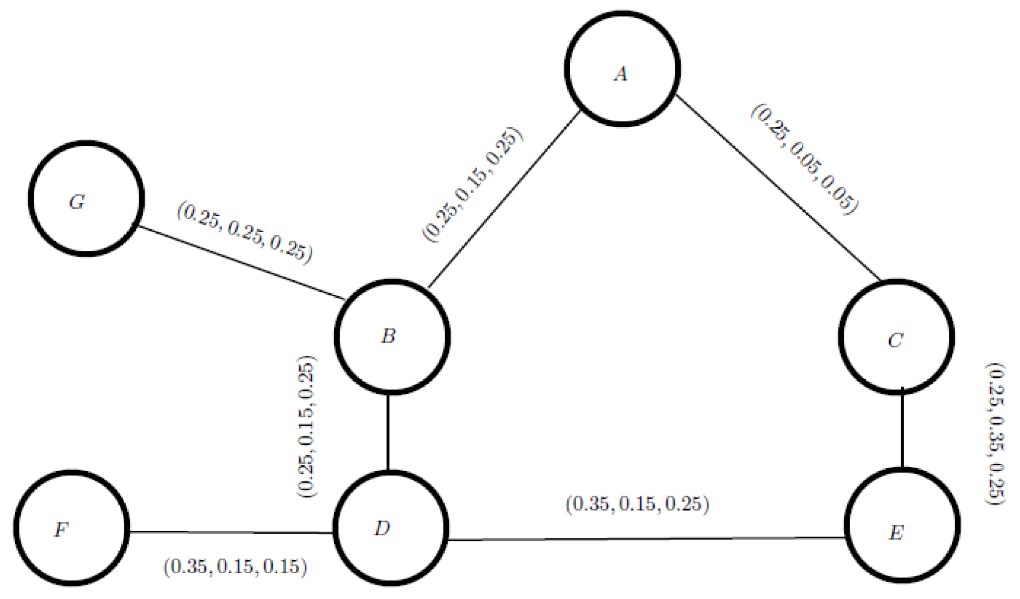
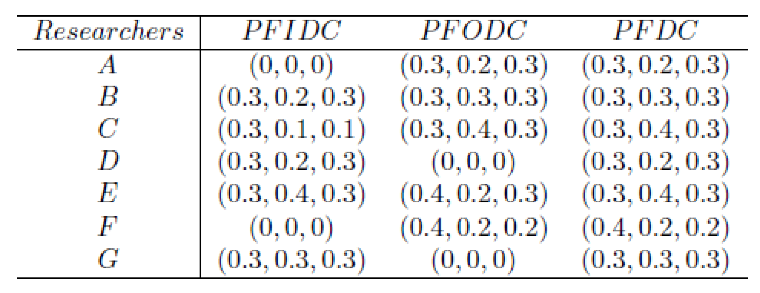
Let $G_{h7}^{\prime }$ = $(V,E_{h7}^{\prime })$ be a directed PFSN of a research team, where V = $\{v_1,v_2,...,v_7\}$ denotes a group of items of seven researchers, and $E_{h8}^{\prime }$ represents a directed PFR between the seven researchers. This social network is shown in Figure 21. Directed PFSN is shown in Figure 22. We determine the PFIDC, PFODC, and PFDC of the researchers. The three-degree values are listed in the table below. To compare the different degree values, we apply PFS’s ranking methods [24,25]. According to the PFS ranking, researcher (node) 4 has the highest PFIDC score value. In the network, this suggests that researcher 4 has a greater level of acceptance and a positive interpersonal relationship. PFODC’s score value for researcher 2 is the highest. This indicates that node 2 can nominate many other researchers.

5. Conclusions

PFG is a generalization of the FG and IFG. The flexibility and comparability of PFGs are much higher than those of FGs and IFGs. A PFG can deal with uncertain problems, whereas an FG and IFG may not be effective in such contexts. In this paper, we describe and explore the MP, SD, RJ, and RP of the PFG. Furthermore, we also discuss the degree and total degree of nodes in the PFG. We present the application of a PFG in digital marketing and social networks. In future work, we will define the following concepts associated with PFGs:

(1)

Lower and upper truncation;

(2)

The degree of lower and upper truncation.