A Study on Nonlinear Dynamic Response of the Large-Span Roof Structure with Suspended Substructure

Abstract

Nowadays, it is common to see large public buildings, e.g., stadiums, with some equipment or substructure suspended from the center of the roof. These substructures will tend to be larger and heavier the more gear is needed, which may have negative impacts on the dynamic performance of the roof structures. In this paper, to explore the dynamic response of a large-span roof structure with a suspended substructure, a real structure model is simplified into a two-degrees-of-freedom system. The essential consideration of nonlinear vibration is elaborated in the equations of motions. Approximate analytical solutions for free and forced vibrations are derived using perturbation methods, while numerical analysis is carried out to validate the solutions. The ratio of linear to nonlinear amplitude is proposed to represent the nonlinear effect of the primary structure, and the nonlinear effect, varying with structural parameters of frequency ratio, mass ratio, excitation ratio, and external force to the primary structure, is investigated. It is shown that internal resonance occurs when the structural frequency ratio is close to 1:2 and that secondary resonance takes place due to certain external excitations; internal resonance and secondary resonance will magnify the amplitude of the primary structure during vibration. Finally, a case of a designed practical dome with a suspended substructure is studied to verify the outcomes from the above research. According to these findings, some design proposals for this type of structure are provided.

1. Introduction

The innovative configuration that some researchers may call a mega-substructure has been proposed to reduce the dynamic response of tall buildings to winds and earthquakes. The concept is that kinetic energy transferred from the primary structure to the substructure is dissipated during oscillation [1]. On the other hand, the tuning mass method is utilized to allow the substructure and primary structure to move in opposite directions so that the vibration of the primary structure is attenuated. Furthermore, optimized parameters of damping and mass ratio could give the structure superior performance [2]. Based on this principle, a suspended floor system is investigated and developed for its simple and effective configuration for earthquake mitigation, which has made it common in the design of high-rise buildings. The famous construction case is the Westcoast Transmission Building in Vancouver (Canada), in which steel cables are used to suspend the main structure as a precaution against seismic effects. Mahmoud et al. [3] discussed the forms of suspension and their seismic performance, arriving at the finding that the frame with a suspended floor outperforms the conventional design. Nakamura et al. [4] proposed a new type of suspension and conducted a shaking table test to verify that the system could have better seismic performance. Engle et al. [5] developed a self-centering isolation floor system, showing that the response of the structure can be reduced by up to 40% by optimizing the design of support and friction. Tatemichi et al. [6] investigated the behavior of suspended floor slabs using hangar rods in high-rise structures, both analytically and experimentally, for the purpose of seismic isolation. Ye et al. [7,8] applied the suspended floor in modular building, studied its dynamic response both numerically and experimentally, and optimized the structure to verify its robustness and aseismic performance. It is to be noted that the aforementioned studies focus mainly on horizontal vibration mitigation, while the literature deals rarely with the vertical performance of suspended structures and their application in large-span roof structures.

For large-span structures, dynamic topics are always popular, especially seismic performance or collapse due to the failure of components. Kato et al. [9,10] investigated the dynamic response of the dome structures, revealing that significant vertical displacement would contribute to the seismic collapse of the large-span domes. Gao et al. [11] also made calculations for a roof structure subjected to an earthquake, and the results showed that the vertical displacement response of the structure is greater than the horizontal displacement response under earthquake. Based on these results, some researchers have sought to employ Tuned Mass Dampers (TMDs) in large-span roof structure design to offer protection against seismic or wind effects. Tang et al. [12] studied the vibration dissipation of a roof structure using multiple TMDs (MTMDs). It was shown that optimum values of frequency width, damping ratio, and mass ratio exist, and those values were determined. Zhou et al. [13] explored the characteristics of MTMDs in a roof structure subjected to wind load, indicating that optimized MTMDs exhibit good dynamic characteristics. Fan [14] introduced the viscous damper system for a braced dome to investigate vibration reduction theoretically and experimentally, the results showing that the vibration-reducing effect of the viscous damper, when incorporated into a braced dome, is significant. Zhou [15] discussed the spring fatigue effect on MTMD optimization, the conclusion of the study indicating that an MTMDs’ control system will reduce its optimal damping performance to meet the spring constraint conditions. From the above studies, additional dampers or devices could improve the performance significantly if the proper parameters are set. In other words, an unfavorable response may occur due to inappropriate parameters.

With the promotion of building functions, roof structures with suspended substructures have become increasingly common. Some stadiums or theatres have lighting equipment or large screens suspended beneath the center of a roof structure, as shown in Figure 1.

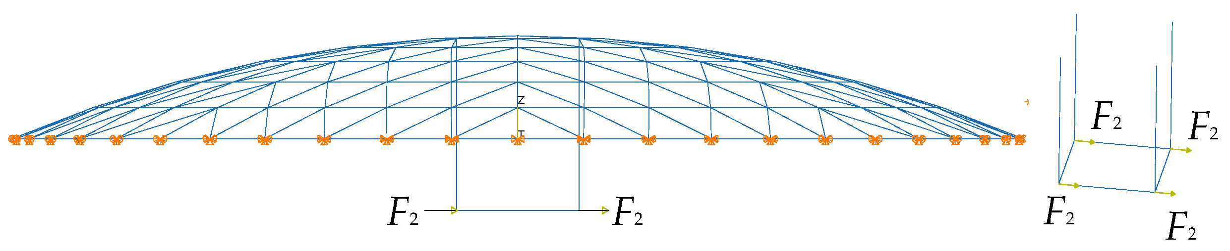
To ensure better views for the audience in some theatres, platform structures are suspended from the center of the roof. For instance, a large-scale circus is being built in Zhangjiajie City, Hunan Province, China. A cable truss system is employed for its large span of 132 m, and it is unusual in having a large heavy stage suspended beneath the roof, as shown in Figure 2. The primary structure is designed to be symmetrical for aesthetic reasons and for reasonable force. As is known from previous studies on large-span structures, the dynamic response especially about the vertical of this kind of structure is critical for estimating the effects of the substructure on the structure of the roof.

As is already known, the roof structure with a substructure functions according to a principle similar to that of a pendulum tuned mass damper (PTMD). Hanging rods provide periodic force for the substructure, the configuration of which is considered simpler than that of a traditional TMD. During analysis, these rods are usually replaced by springs, and the substructure can be regarded as a normal TMD. Gerges [16] made the assumption that the pendulum angle was negligibly small in the equation of motion, and optimal parameters of PTMD were determined under random white noise excitation. Deraemaeker and Soltani [17] applied the equal peak method to derive the optimum length and damping of the pendulum. Chulahwat and Mahmoud [3,18] explored the dynamic response of a steel frame with a suspended floor, with hanger rods simplified into springs representing stiffness of the substructure. In the same way, Ye [7,8] used an equivalent spring to simulate connections between the primary structure and modular substructure when conducting seismic performance analysis. There are other forms of TMDs derived from PTMDs. Matta [19,20] studied the rolling PTMD analytically for its practical application in roof gardens, with results showing that the rolling PTMD can be a good alternative to traditional TMDs on account of its advantages in terms of flexibility and multitasking.

In general, linear models of PTMDs always have enough accuracy at negligibly small pendulum angles. In fact, nonlinear effects of PTMDs exist where severe oscillations take place. Roffel [21] explored three-dimensional motions of PTMDs coupled nonlinearly with flexible primary structure. Nonlinear 3D and planar models were established and studied. It was shown that the planar model has errors of 9% relative to the 3D model with low mass ratios, and that maximum error reaches up to 20% between the two models when mass ratios increase. Yurchenko [22] concluded that motions of the primary structure could excite suspension points that may cause nonlinear parametric vibration of PTMDs, and hence considered it a parametrically excited system. Bajaj [23] investigated a two-degrees-of-freedom autoparametric nonlinear vibration absorber system, whose complex nonlinear vibrations, such as bifurcations and chaos, might happen at some excitation frequencies and forcing amplitudes. Song [24] used the harmonic balance method to analytically explore the characteristics and stabilities of the vibration response of a parametrically excited pendulum system. Areas of stable and unstable solutions were obtained. Majcher [25] studied the parametric vibration of PTMD in high-rise structures numerically, with results indicating the vertical ground motion transmitted to pendulum suspension points may lead to parametric resonance in the system. It can be appreciated from the aforementioned studies that it is necessary to nonlinearly analyze large-span roof structures with suspended substructures that vibrate vertically to obtain more exact results.

Few current studies are focused on large-span roof structures with large and heavy suspended substructures and on the dynamic performance of this kind of structure, which is here discussed analytically for its nonlinearity. This research is the first to investigate the nonlinear dynamic characteristics of large-span roof structures with suspended substructures, by simplifying the model from a real complex structure into a two-degrees-of-freedom system to establish the equations of motions. The distinction between nonlinear and linear vibrations is explored in the equations, and nonlinear analysis is shown to be necessary and then carried out in the analysis that follows. Analytical solutions of free and forced vibrations are obtained using multiscale perturbation methods, and some structural frequency parameters which may lead to amplified vibration of the primary structure are discussed. A nonlinear effect represented in terms of the ratio of nonlinear to linear amplitude is discussed using parametric analysis. Lastly, nonlinear free and forced vibration analysis of a roof structure with a substructure is conducted to verify the conclusions obtained above. Based on these studies, some suggestions are provided for this kind of structure.

2. Simplified Model and Dynamic Equations

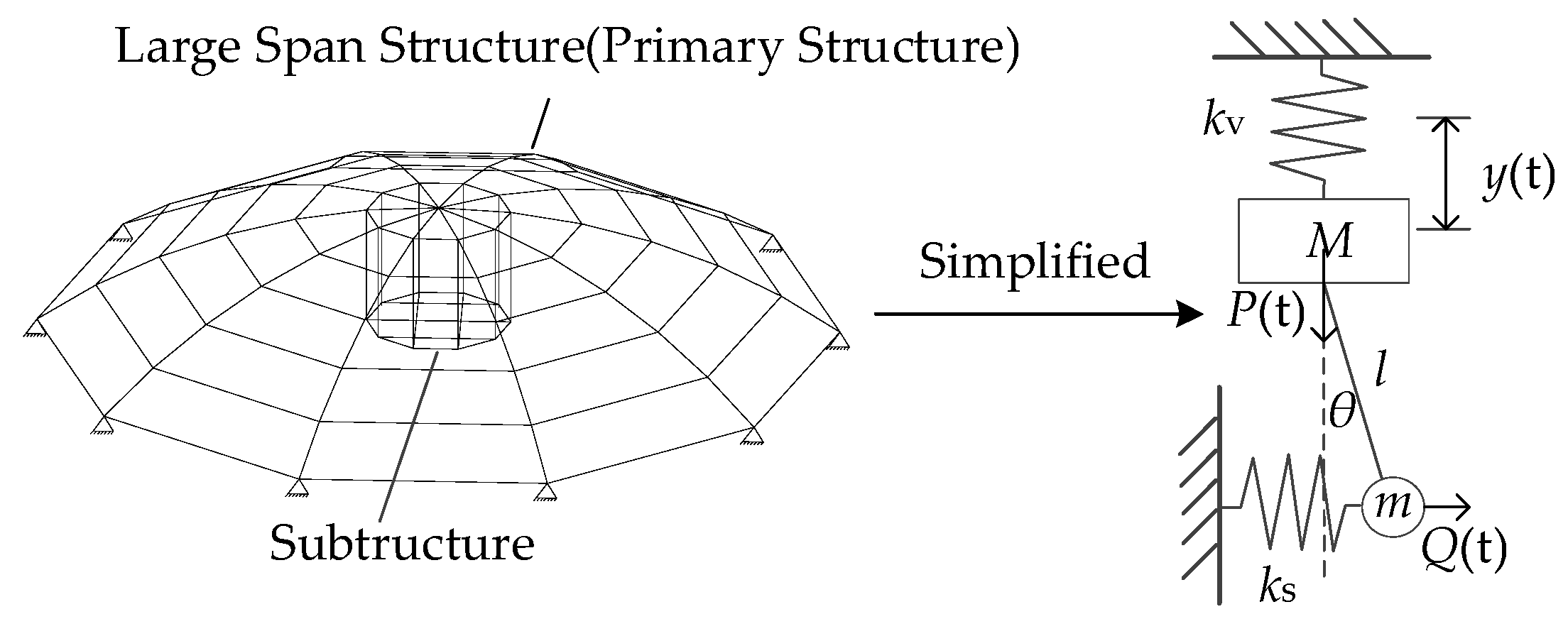
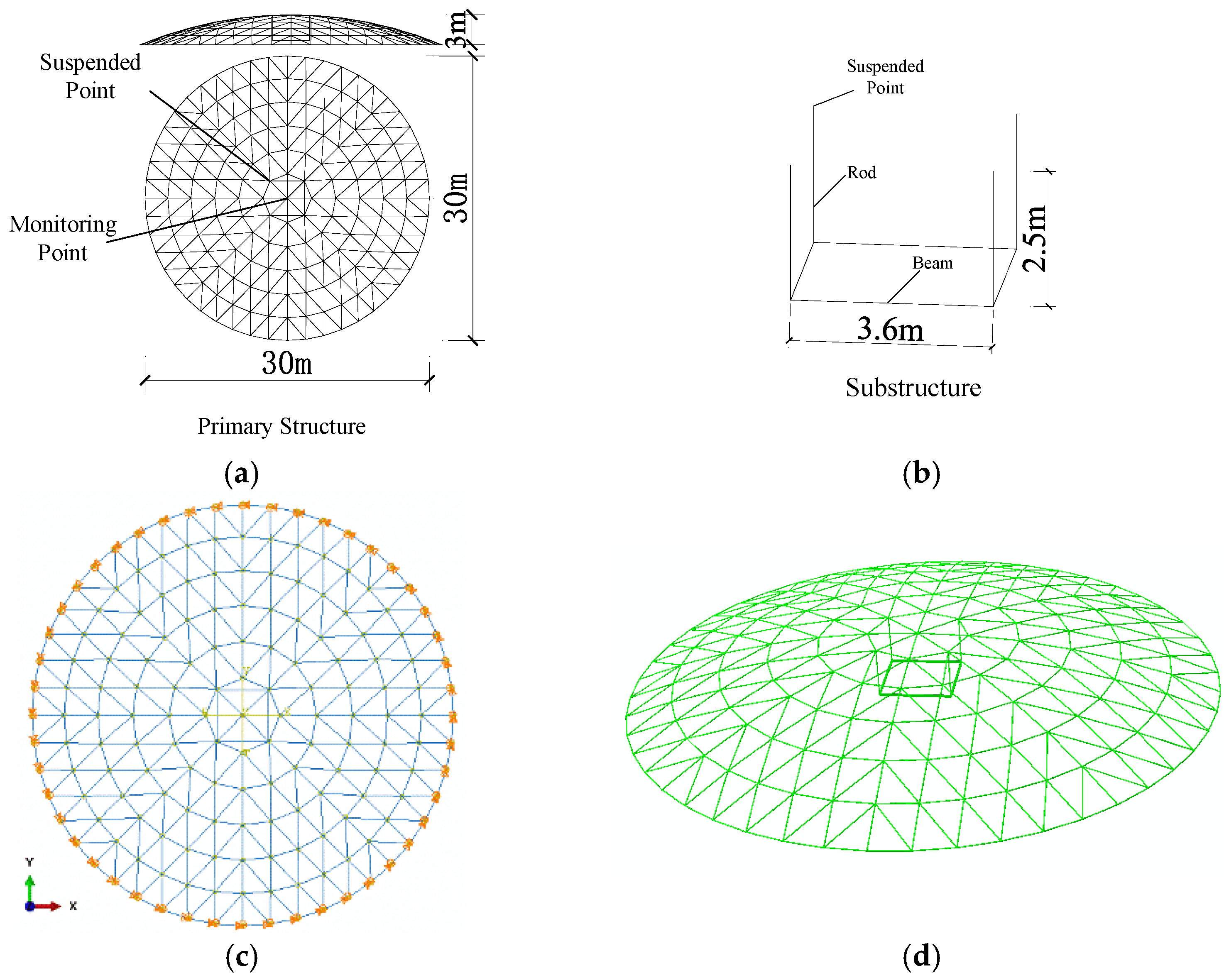
As has been discussed in the aforementioned publications, large-span structures are always vulnerable to vertical excitations. In the analyses of large-span structures, more attention has been paid to the vertical response. Moreover, analytical solutions and inside regulations of nonlinear vibrations may not be obtained when considering the practical models with multiple degrees of freedom. For these reasons, a simplified model of a large-span roof structure with a suspended substructure is proposed, as is diagramed in Figure 3. The roof structure denoted by a lattice is the primary structure. It can be simplified into a pendulum-type model with two degrees of freedom when only the vertical vibration of the primary structure and the swing of the substructure are taken into consideration.

According to Lagrange’s equation [26], undamped equations of motions with nonlinear terms at the right-hand side can be written as:

$$\begin{array}{l}M\ddot{y}+k_{v}y=-ml\ddot{\theta }\sin \theta -ml{\dot{\theta }}^2\cos \theta -m\ddot{y}+P(t)\\ ml\ddot{\theta }+\left(mg+k_{\mathrm{s}}l\right)\sin \theta =-m\ddot{y}\sin \theta +Q(t)\end{array}$$

(1)

where M, m = mass of the primary structure and the substructure, respectively; k_v = total vertical stiffness of the primary structure; y = vertical displacement of the primary structure; θ, l = angle and length of the pendulum, respectively; k_s = total lateral stiffness of the hanger rods; P(t), Q(t) = external excitations to the primary structure and substructure, respectively.

Taylor expansion is carried out for the trigonometric terms ignoring higher-order terms, so that sin θ and cos θ can be approximated by θ and 1, respectively. Nonlinear terms are multiplied by the perturbation parameter ε [27], indicating that the linear system is disturbed by the nonlinear terms. The equations become:

$$\begin{array}{l}\left(M+m\right)\ddot{y}+k_{v}y=\epsilon \left(-ml\ddot{\theta }\theta -ml{\dot{\theta }}^2\right)+P(t)\\ ml\ddot{\theta }+\left(mg+k_{\mathrm{s}}l\right)\theta =-\epsilon m\ddot{y}\theta +Q(t)\end{array}$$

(2)

Terms at the left-hand side of Equation (2) are linear. For the simplified model, if vibration is regarded as linear, the equations reduce to Equation (3) (ε = 0):

$$\begin{array}{l}\left(M+m\right)\ddot{y}+k_{v}y=P(t)\\ ml\ddot{\theta }+\left(mg+k_{\mathrm{s}}l\right)\theta =Q(t)\end{array}$$

(3)

It can be found that in Equation (3), interaction between the primary structure and substructure is eliminated when the nonlinear terms are ignored, so that vibrations are independent of each other, which means that the substructure has no effect on the primary structure. In fact, the nonlinear terms in Equation (2) are a secondary excitation to the original linear system, such that some dynamic properties can be ignored during linear analysis of the structure. The dynamic problem of the large-span roof with a suspended substructure is nonlinear in essence. This nonlinearity is exactly what is investigated in this paper.

3. Free Vibration Characteristics Analysis

Free vibration is nonlinear according to the studies above. Let P(t), Q(t) = 0 in Equation (2). Then, free vibration can be quantified by the following equation:

$$\begin{array}{l}\left(M+m\right)\ddot{y}+k_{v}y=\epsilon \left(-ml\ddot{\theta }\theta -ml{\dot{\theta }}^2\right)\\ ml\ddot{\theta }+\left(mg+k_{\mathrm{s}}l\right)\theta =-\epsilon m\ddot{y}\theta \end{array}$$

(4)

Vertical frequency of the primary structure and swing frequency of the substructure, respectively, are:

$${\omega }_{10}=\sqrt{\frac{k_v}{M+m}}$$

(5a)

$${\omega }_{20}=\sqrt{\frac{g}{l}+\frac{k_s}{m}}$$

(5b)

Substitute Equation (5a,b) into Equation (4) and reduce them to:

$$\begin{array}{l}\ddot{y}+{\omega }_{10}^{2}y=\epsilon \left(-\mu l\ddot{\theta }\theta -\mu l{\dot{\theta }}^2\right)\\ \ddot{\theta }+{\omega }_{20}^2\theta =-\epsilon \frac{m\ddot{y}\theta }{l}\end{array}$$

(6)

where $\mu =\frac{m}{M+m}$.

The multiscale perturbation method [20] is applied to solve Equation (6). The multiscale method is a significant perturbation method for solving nonlinear dynamic problems analytically. The vibrations of the structure are assumed to consist of the original linear solution and the nonlinear solution, and the nonlinear solution is multiplied by the perturbation parameters which represent the perturbation of the nonlinearity. This perturbation performs at different time scales related to the perturbation parameter. Equations can be solved in each time scale.

Assuming that y and θ consist of the original linear solution (y₀, θ₀) and nonlinear solution (y₁, θ₁):

$$\begin{array}{l}y=y_0(T_0,T_1)+\epsilon y_1(T_0,T_1)\\ \theta ={\theta }_0(T_0,T_1)+\epsilon {\theta }_1(T_0,T_1)\end{array}$$

(7)

where y₀, θ₀, y₁, and θ₁ can be considered as functions of T₀, T₁. Scales of time T₀, T₁ and real time t can be related as follows:

$$T_n={\epsilon }^{n}t,n=0,1$$

(8)

Substitute Equations (7) and (8) into Equation (6) to derive the below equations in each time scale:

$$\begin{array}{ll}{\epsilon }^0:& D_0^2{y}_0+{\omega }_{{}_{10}}^2{y}_0=0\\ & D_0^2{\theta }_0+{\omega }_{{}_{20}}^2{\theta }_0=0\end{array}$$

(9a)

$$\begin{array}{ll}{\epsilon }^1:& D_0^2{y}_1+{\omega }_{{}_{10}}^2{y}_1=-2D_0{D}_1{y}_0-l\mu \left({\theta }_0{D}_0^2{\theta }_0+{\left(D_0{\theta }_0\right)}^2\right)\\ & D_0^2{\theta }_1+{\omega }_{{}_{20}}^2{\theta }_1=-2D_0{D}_1{\theta }_0-{\theta }_0{D}_0^2{y}_0/l\end{array}$$

(9b)

where $D_i=\frac{\partial }{\partial T_i}$ is the (first order) differential operator.

Solutions of y₀ and θ₀ in Equation (9a) can be assumed as:

$$\begin{array}{l}{y}_0=A{e}^{i{\omega }_{10}{T}_0}+\overline{A}{e}^{-i{\omega }_{10}{T}_0}\\ {\theta }_0=B{e}^{i{\omega }_{20}{T}_0}+\overline{B}{e}^{-i{\omega }_{20}{T}_0}\end{array}$$

(10)

where A and B are complex amplitudes; $\overline{A}$ and $\overline{B}$ are conjugative amplitudes of A and B, respectively; all of them are functions of T₁; i is the imaginary unit.

Substitute Equation (10) into Equation (9b):

$$\begin{array}{l}{D}_0^2{y}_1+{\omega }_{{}_{10}}^2{y}_1=-2\mathrm{i}{\omega }_{10}{A}^{\prime }{\mathrm{e}}^{\mathrm{i}{T}_0{\omega }_{10}}+2B^2{\mathrm{e}}^{2\mathrm{i}{T}_0{\omega }_{20}}l\mu {\omega }_{20}^2+cc\\ D_0^2{\theta }_1+{\omega }_{{}_{20}}^2{\theta }_1=-2\mathrm{i}{\omega }_{20}{B}^{\prime }{\mathrm{e}}^{\mathrm{i}{T}_0{\omega }_{20}}+\frac{AB{\mathrm{e}}^{\mathrm{i}{T}_0\left({\omega }_{10}+{\omega }_{20}\right)}{\omega }_{10}^2}{l}+\frac{\overline{B}{\mathrm{e}}^{-\mathrm{i}{T}_0\left({\omega }_{10}-{\omega }_{20}\right)}A{\omega }_{10}^2}{l}+cc\end{array}$$

(11)

where A′ and B′ are derivatives of A and B, respectively, with respect to time scale T₁; cc denotes the conjugation of the previous items; $-2\mathrm{i}{\omega }_{10}{A}^{\prime }{\mathrm{e}}^{\mathrm{i}{T}_0{\omega }_{10}}+cc$ and $-2\mathrm{i}{\omega }_{20}{B}^{\prime }{\mathrm{e}}^{\mathrm{i}{T}_0{\omega }_{20}}+cc$ are secular terms.

As shown in Equation (11), except for the secular terms, y₁ is driven by the term with a frequency of 2ω₂₀, and θ₁ is excited at frequencies of ω₁₀ − ω₂₀ and ω₁₀ + ω₂₀. Notice that as ω₁₀ approaches 2ω₂₀, the secondary excitation frequency gets close to the original linear frequency, leading to internal resonance of y₁ and θ₁. The internal resonance relation is shown as:

$${\omega }_{10}\approx 2{\omega }_{20}$$

(12)

Solutions of Equation (11) can be separated into resonance solutions and general solutions. However, the latter are given in this study. Let the secular terms equal zero. Then A and B are obtained to solve y₀, θ₀, y₁, and θ₁ subsequently. The final solutions are:

$$\begin{array}{l}y=\left(u_0-\frac{\mu v_0^{2}l{\omega }_{20}^2}{\left({\omega }_{10}^2-4{\omega }_{20}^2\right)}\right)\cos \left({\omega }_{10}t\right)+\frac{\mu v_0^{2}l{\omega }_{20}^2}{\left({\omega }_{10}^2-4{\omega }_{20}^2\right)}\cos \left(2{\omega }_{20}t\right)\\ \theta =\left(v_0-\frac{u_0{v}_0{\omega }_{10}^2}{2l\left({\omega }_{20}^2-{\left({\omega }_{20}-{\omega }_{10}\right)}^2\right)}-\frac{u_0{v}_0{\omega }_{10}^2}{2l\left({\omega }_{20}^2-{\left({\omega }_{20}+{\omega }_{10}\right)}^2\right)}\right)\cos \left({\omega }_{20}t\right)\\ +\frac{u_0{v}_0{\omega }_{10}^2}{2l\left({\omega }_{20}^2-{\left({\omega }_{20}-{\omega }_{10}\right)}^2\right)}\cos \left(\left({\omega }_{20}-{\omega }_{10}\right)t\right)+\frac{u_0{v}_0{\omega }_{10}^2}{2l\left({\omega }_{20}^2-{\left({\omega }_{20}+{\omega }_{10}\right)}^2\right)}\cos \left(\left({\omega }_{20}+{\omega }_{10}\right)t\right)\end{array}$$

(13)

where u₀ and v₀ are initial displacement and pendulum angle of the primary structure and substructure, respectively.

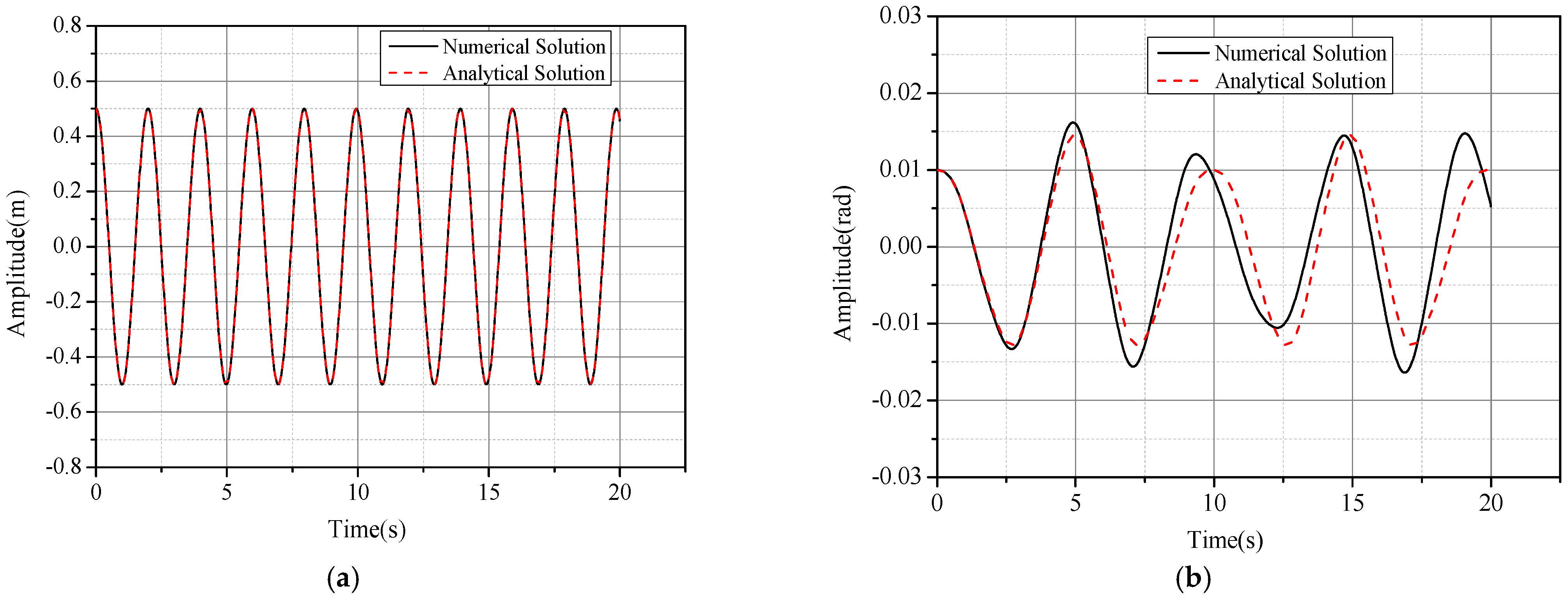
From Equation (13), higher-order harmonics in nonlinear solutions can be derived. Numerical solution is obtained using the Runge–Kutta method for integration. Comparison between the numerical and analytical solutions is displayed in Figure 4, which indicates that time history curves of both solutions for the primary structure have high coincidence, while there is a small deviation for the substructure. The solutions obtained above can be proven to be valid.

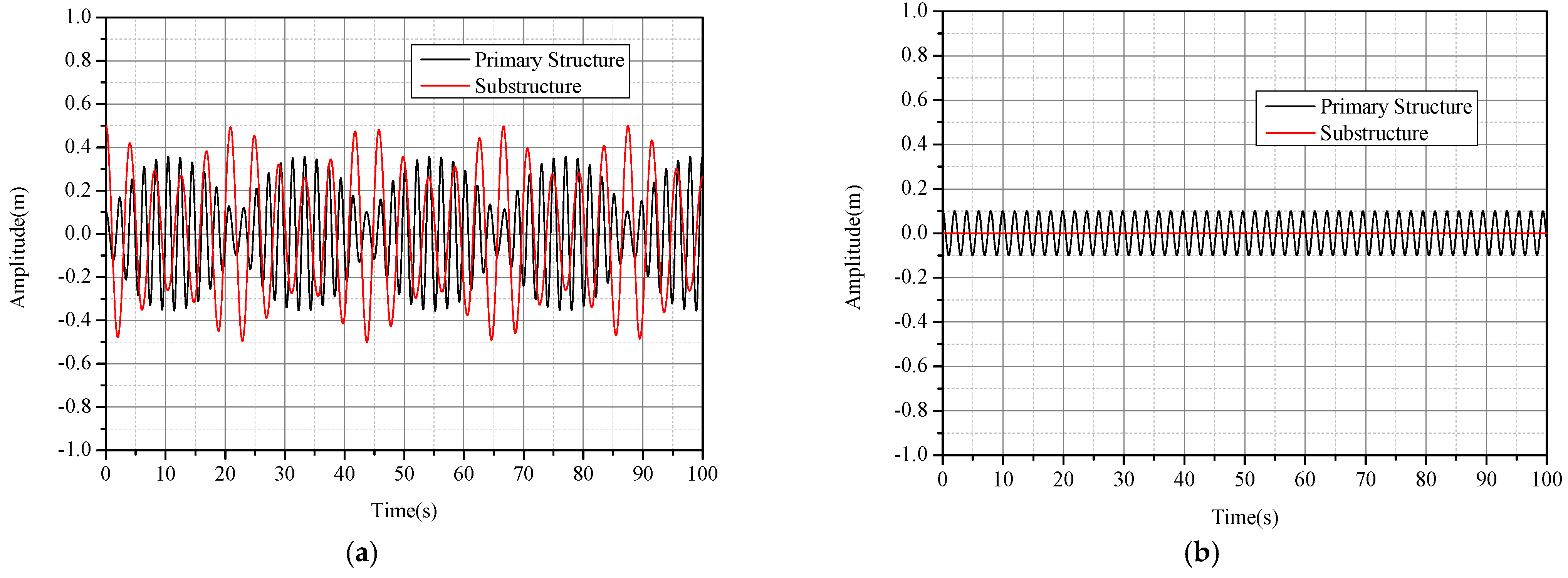
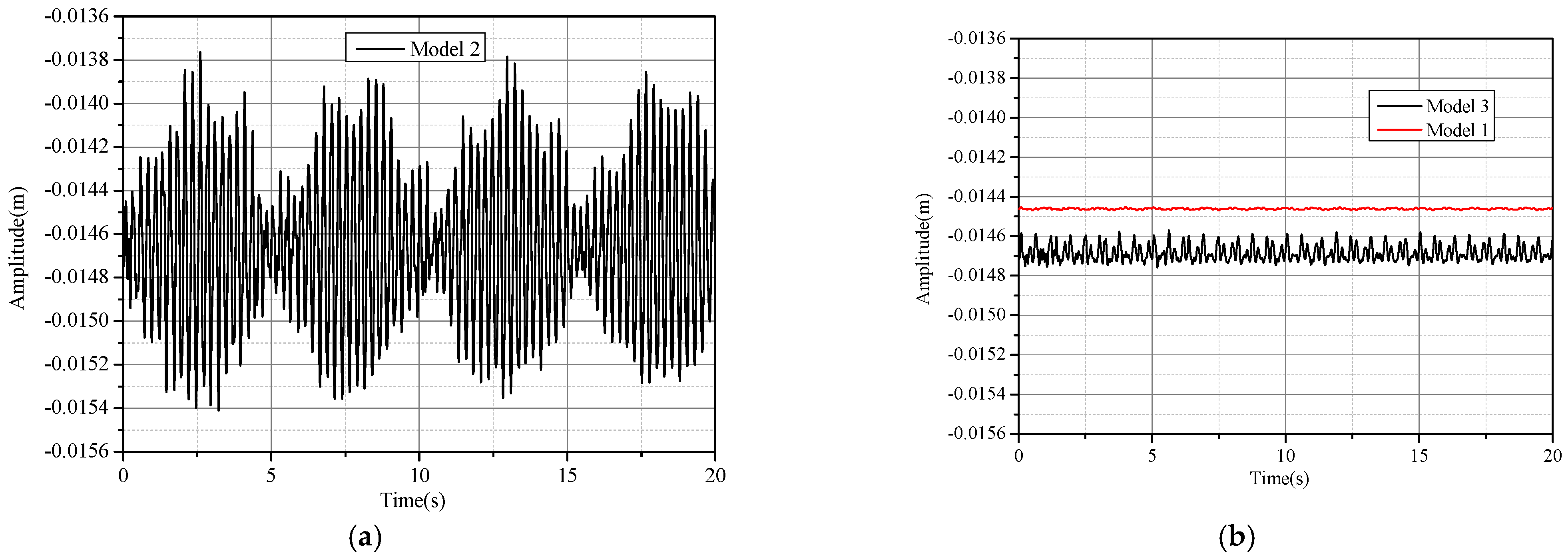
The time history response of the structure with structural parameters set up for ω₁₀ ≈ 2ω₂₀ is shown in Figure 5a. It can be seen that as the vertical displacement of the primary structure increases from an initial displacement of 0.1 m to 0.3 m within about 10 s, the pendulum angle of the substructure decreases, that is, the vertical vibration of the primary structure strengthens, while the swing of the substructure weakens, which manifests internal resonance as energy is transmitted between these two vibration modes. Notice that when v₀ = 0 in Equation (13) vibrations reduce to the linear form of Equation (14). As shown in Figure 5b, vibrations of the substructure have come to a full stop, while vibration of the primary structure continues undisturbed with an amplitude much smaller than that of the nonlinear vibration. Conclusions can be drawn that the swing of the substructure is vital to nonlinearity.

$$\begin{array}{l}y=u_0\cos \left({\omega }_{10}t\right)\\ \theta =0\end{array}$$

(14)

4. Nonlinear Analysis in Forced Vibration

Evidently, nonlinearity makes the vibration more complicated; some frequencies critical to structure, which may strengthen the vibration of the primary structure, are ignorable when linear vibration is considered alone. In this section, the structural response to external excitations is studied.

Harmonic excitations P(t) and Q(t) are adopted herein and are converted into complex forms:

$$\begin{array}{l}P(t)=F_1{e}^{i{\mathrm{\Omega }}_{1}t}\\ Q(t)=F_2{e}^{i{\mathrm{\Omega }}_{2}t}\end{array}$$

(15)

where Ω₁ and Ω₂ are (radian) frequencies of excitations to the primary structure and substructure, respectively; F₁ and F₂ are corresponding forcing amplitudes.

For brevity, a similar procedure is omitted to give the following equations with external excitations in each time scale:

$$\begin{array}{ll}{\epsilon }^0:& D_0^2{y}_0+{\omega }_{{}_{10}}^2{y}_0=f_1{e}^{j{\mathrm{\Omega }}_{1}t}\\ & D_0^2{\theta }_0+{\omega }_{{}_{20}}^2{\theta }_0=f_2{e}^{j{\mathrm{\Omega }}_{2}t}\end{array}$$

(16a)

$$\begin{array}{ll}{\epsilon }^1:& D_0^2{y}_1+{\omega }_{{}_{10}}^2{y}_1=-2D_0{D}_1{y}_0-l\mu \left({\theta }_0{D}_0^2{\theta }_0+{\left(D_0{\theta }_0\right)}^2\right)\\ & D_0^2{\theta }_1+{\omega }_{{}_{20}}^2{\theta }_1=-2D_0{D}_1{\theta }_0-{\theta }_0{D}_0^2{y}_0/l\end{array}$$

(16b)

where $f_1=\frac{F_1}{M+m}$; $f_2=\frac{F_2}{ml}$.

As displayed in Equation (16a), the primary resonant frequencies in the linear vibration for y₀ and θ₀ can be derived as:

$${\mathrm{\Omega }}_1\approx {\omega }_{10}$$

(17a)

$${\mathrm{\Omega }}_2\approx {\omega }_{20}$$

(17b)

Solutions of y₀ and θ₀ in Equation (16a) can be assumed as:

$$\begin{array}{l}{y}_0=A{e}^{i{\omega }_{10}{T}_0}+\overline{A}{e}^{-i{\omega }_{10}{T}_0}+P_1{e}^{i{\mathrm{\Omega }}_1{T}_0}+{\overline{P}}_1{e}^{-i{\mathrm{\Omega }}_1{T}_0}\\ {\theta }_0=B{e}^{i{\omega }_{20}{T}_0}+\overline{B}{e}^{-i{\omega }_{20}{T}_0}+Q_1{e}^{i{\mathrm{\Omega }}_2{T}_0}+{\overline{Q}}_1{e}^{-i{\mathrm{\Omega }}_2{T}_0}\end{array}$$

(18)

where $P_1=\frac{f_1}{2\left({\omega }_{10}^2-{\mathrm{\Omega }}_1^2\right)}$; $Q_1=\frac{f_2}{2\left({\omega }_{20}^2-{\mathrm{\Omega }}_2^2\right)}$; A, B, $\overline{A}$, $\overline{B}$ can all be deemed as functions of T₁.

Substitute Equation (18) into Equation (16b):

$$\begin{array}{l}{D}_0^2{y}_1+{\omega }_{10}^2{y}_1=-2\mathrm{i}{\omega }_{10}{A}^{\prime }{\mathrm{e}}^{\mathrm{i}{T}_0{\omega }_{10}}+2B^{2}l\mu {\omega }_{20}^2{\mathrm{e}}^{2\mathrm{i}{T}_0{\omega }_{20}}\\ +Bl{Q}_1\mu {\left({\omega }_{20}+{\mathrm{\Omega }}_2\right)}^2{\mathrm{e}}^{\mathrm{i}\left({\mathrm{\Omega }}_2+{\omega }_{20}\right)T_0}+\overline{B}l{Q}_1\mu {\left({\omega }_{20}-{\mathrm{\Omega }}_2\right)}^2{\mathrm{e}}^{\mathrm{i}\left({\mathrm{\Omega }}_2-{\omega }_{20}\right)T_0}\\ +2l{Q}_1^2\mu {\mathrm{\Omega }}_2^2{\mathrm{e}}^{2\mathrm{i}{\mathrm{\Omega }}_2{T}_0}+cc\\ D_0^2{\theta }_1+{\omega }_{20}^2{\theta }_1=-2\mathrm{i}{\omega }_{20}{B}^{\prime }{\mathrm{e}}^{\mathrm{i}{T}_0{\omega }_{20}}+\frac{AB{\omega }_{10}^2}{l}{\mathrm{e}}^{\mathrm{i}\left({\omega }_{10}+{\omega }_{20}\right)T_0}+\frac{A\overline{B}{\omega }_{10}^2}{l}{\mathrm{e}}^{\mathrm{i}\left({\omega }_{10}-{\omega }_{20}\right)T_0}\\ +\frac{\overline{A}{Q}_1{\omega }_{10}^2}{l}{\mathrm{e}}^{\mathrm{i}\left({\mathrm{\Omega }}_2-{\omega }_{10}\right)T_0}+\frac{A{Q}_1{\omega }_{10}^2}{l}{\mathrm{e}}^{\mathrm{i}\left({\mathrm{\Omega }}_2+{\omega }_{10}\right)T_0}+\frac{\overline{B}{P}_1{\mathrm{\Omega }}_1^2}{l}{\mathrm{e}}^{\mathrm{i}\left({\mathrm{\Omega }}_1-{\omega }_{20}\right)T_0}\\ +\frac{B{P}_1{\mathrm{\Omega }}_1^2}{l}{\mathrm{e}}^{\mathrm{i}\left({\mathrm{\Omega }}_1+{\omega }_{20}\right)T_0}+\frac{P_1{Q}_1{\mathrm{\Omega }}_1^2}{l}{\mathrm{e}}^{\mathrm{i}\left({\mathrm{\Omega }}_2+{\mathrm{\Omega }}_1\right)T_0}+\frac{{\overline{P}}_1{Q}_1{\mathrm{\Omega }}_1^2}{l}{\mathrm{e}}^{\mathrm{i}\left({\mathrm{\Omega }}_2-{\mathrm{\Omega }}_1\right)T_0}+cc\end{array}$$

(19)

It is found that the external excitations make the equations more complicated. Except for the secular terms $-2\mathrm{i}{\omega }_{10}{A}^{\prime }{\mathrm{e}}^{\mathrm{i}{T}_0{\omega }_{10}}+cc$, the frequencies resulting in resonance for y₁ from Equation (19) can be expressed, respectively, as:

$${\omega }_{10}\approx 2{\omega }_{20}$$

(20a)

$${\mathrm{\Omega }}_2\approx {\omega }_{10}+{\omega }_{20}\mathrm{or}{\mathrm{\Omega }}_2\approx \left|{\omega }_{20}-{\omega }_{10}\right|$$

(20b)

$${\mathrm{\Omega }}_2\approx {\omega }_{10}/2$$

(20c)

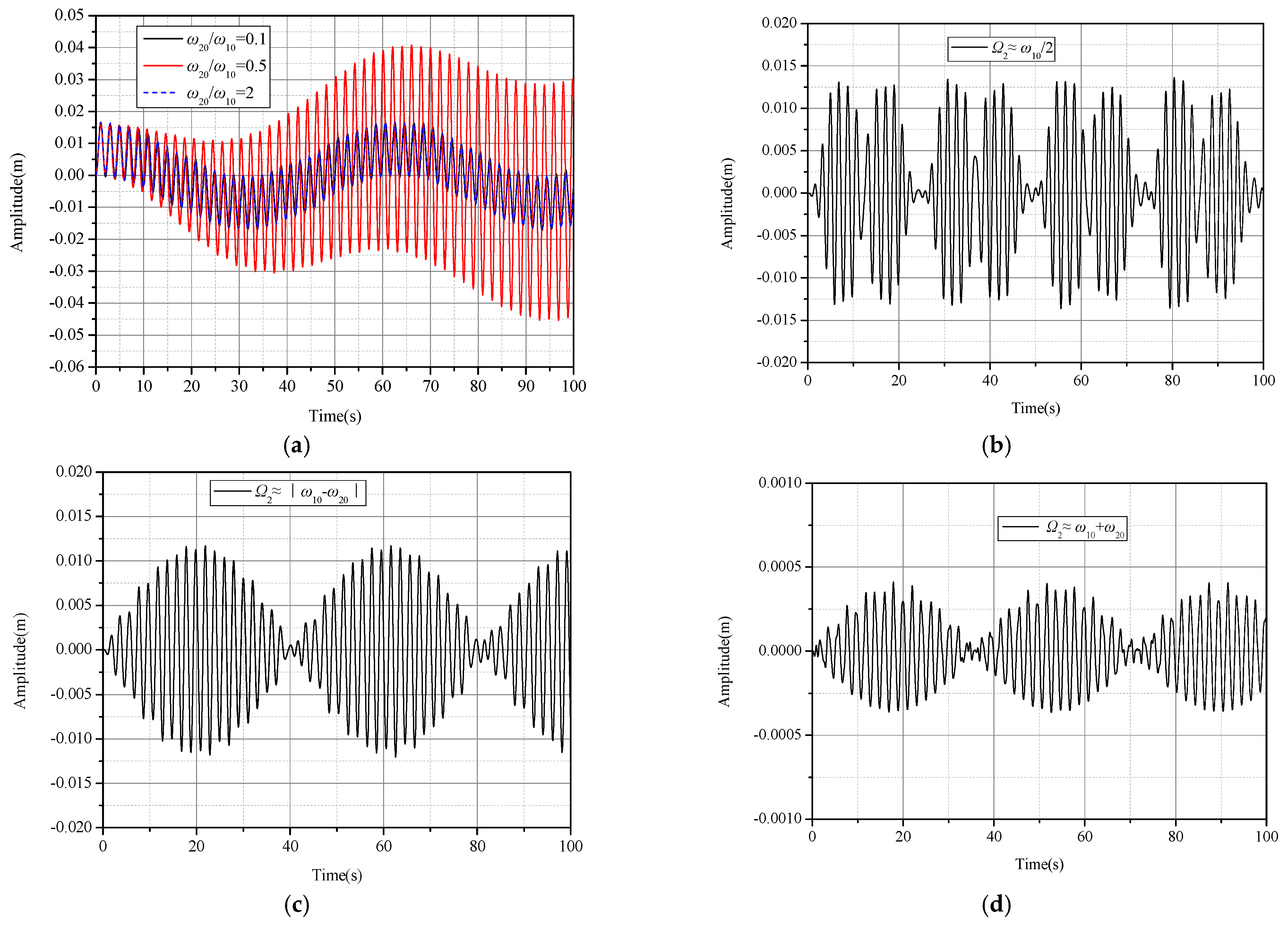
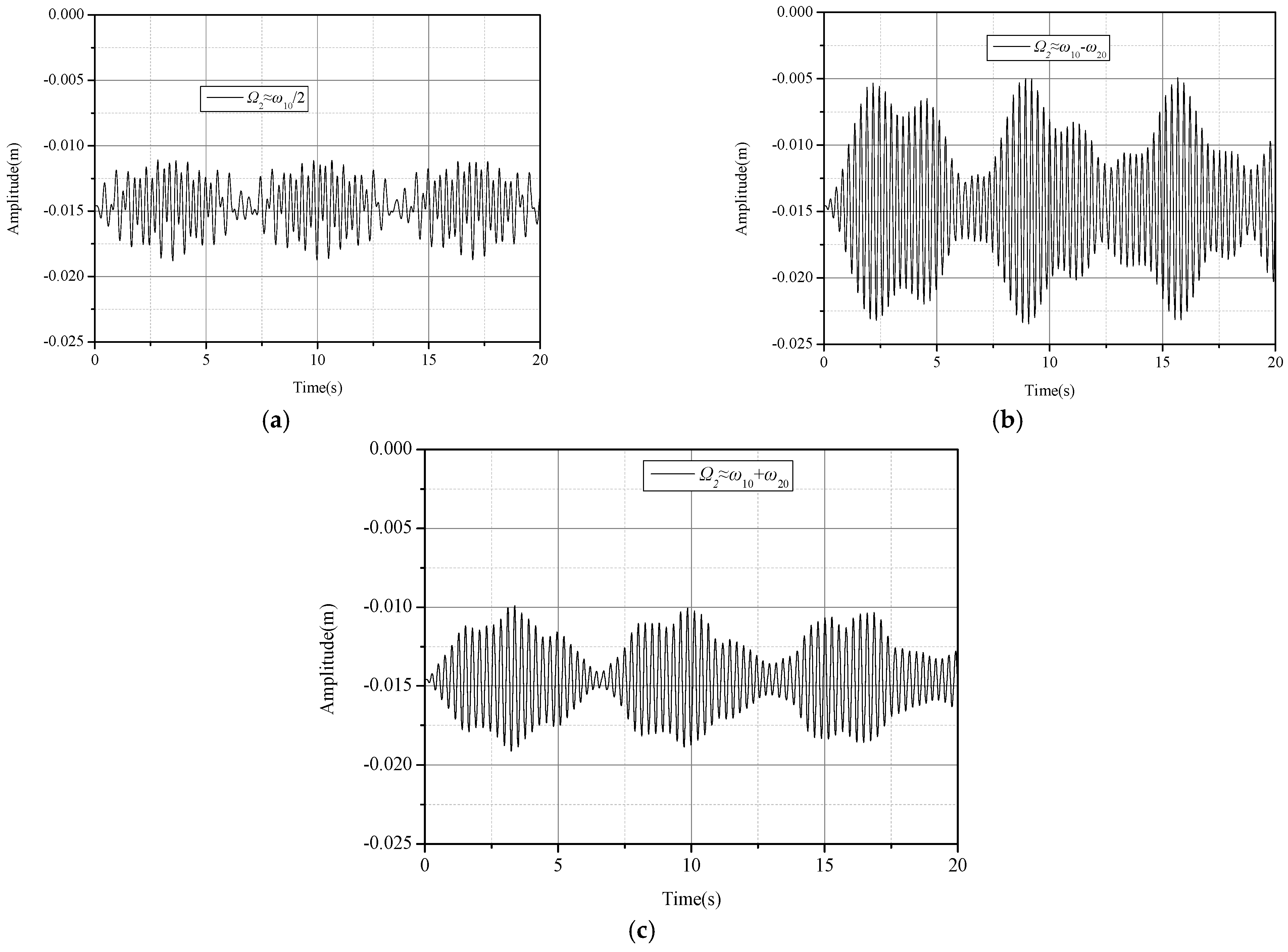
Equation (20a) reflects the frequency relation of internal resonance as in a previous study. Equation (20b,c) reflect the secondary resonance relation for y₁. Time history results of the primary structure subjected to specific excitations are shown in Figure 6a. When the frequency ratio of substructure to primary structure is near 0.5, the vertical displacement of the primary structure, which is amplified during the vibration, is unstable and divergent, while the other structural frequency ratio coincides with steady-state vibration. As frequencies of excitations to the substructure approach the secondary resonance frequency referred to in Equation (20b,c), amplitudes of vibration of the primary structure are augmented to different degrees. As illustrated in Figure 6b, the frequency of excitations to the substructure in Equation (20c) presents the amplitude of the primary structure as a “beat” oscillation [28], which means that the external frequency is close to the structural frequency. As is shown in Figure 6d, the excitation frequency of the substructure, ω₁₀ + ω₂₀, in Equation (20b) shows the minimum amplification of vibration, since the excitation frequency is too high relative to the linear frequency of the substructure, which is hardly excited, making the final result small.

Finally, the general solution is:

$$\begin{array}{l}y=c_1\cos {\omega }_{10}t+c_2\cos {\mathrm{\Omega }}_{1}t+c_3\cos 2{\omega }_{20}t+c_4\cos \left({\mathrm{\Omega }}_2+{\omega }_{20}\right)t+c_5\cos \left({\mathrm{\Omega }}_2-{\omega }_{20}\right)t\\ +c_6\cos 2{\mathrm{\Omega }}_{2}t\\ \theta =d_1\cos {\omega }_{20}t+d_2\cos {\mathrm{\Omega }}_{2}t+d_3\cos \left({\omega }_{10}+{\omega }_{20}\right)t+d_4\cos \left({\omega }_{10}-{\omega }_{20}\right)t+d_5\cos \left({\mathrm{\Omega }}_2-{\omega }_{10}\right)t\\ +d_6\cos \left({\mathrm{\Omega }}_2+{\omega }_{10}\right)t+d_7\cos \left({\mathrm{\Omega }}_1-{\omega }_{20}\right)t+d_8\cos \left({\mathrm{\Omega }}_1+{\omega }_{20}\right)t+d_9\cos \left({\mathrm{\Omega }}_2+{\mathrm{\Omega }}_1\right)t\\ +d_{10}\cos \left({\mathrm{\Omega }}_2-{\mathrm{\Omega }}_1\right)t\end{array}$$

(21)

where c₁, c₂, … c₆, d₁, d₂, … d₁₀ are coefficients of the harmonic terms referred to in Appendix A.

The linear solutions of the structure subjected to the same excitation are given as:

$$\begin{array}{l}y=e_1\cos {\omega }_{10}t+e_2\cos {\mathrm{\Omega }}_{1}t\\ \theta =f_1\cos {\omega }_{20}t+f_2\cos {\mathrm{\Omega }}_{2}t\end{array}$$

(22)

where e₁, e₂, f₁, and f₂ are referred to in Appendix A.

It is revealed that the external force can introduce more harmonics into the nonlinear system, which is different from the linear forced vibration. Secondary frequencies should be taken into account for forced vibration analysis.

To assess the validity of solutions subjected to different excitations, the amplitude ratio of numerical to analytical results is discussed. Parameters of the calculation model refer to the practical engineering structure, as shown in

Table 1. Parameters of practical model.

M (kg)	m (kg)	kv (N/m)	l (m)	ks (N/m)	ω10 (rad/s)	m/M	ω20/ω10	Time (s)
105	5000	5.5 × 106	3.29	104	7.25	0.05	0.3	100

.

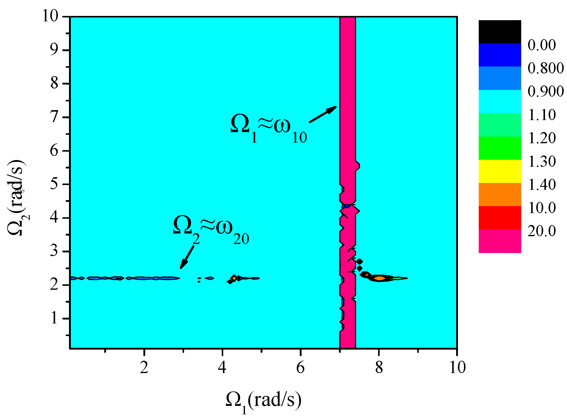
The contour of the amplitude ratio to distinct frequencies of excitation is pictured in Figure 7. It is shown that the ratio ranges almost between 0.9 and 1.1; as excitation frequencies approach the resonant frequency of the primary structure or substructure, deviation becomes obvious. The conclusion can be drawn that the analytical solution is accurate enough, and hence has a high efficiency for general excitation frequencies except for resonant frequencies.

5. Nonlinear Effect Analysis

As shown in the above studies, nonlinear solutions of the structure are more complicated, with many additional harmonics included in the final solutions. However, it can be found that nonlinearity is obviously affected by structural parameters, among which excitations to the primary structure and substructure are critical factors for nonlinearity. External forcing amplitude also accounts markedly for the nonlinearity of the structure. Furthermore, as excitations to the primary structure are strengthened, the nonlinearity due to the same amplitude of external force on the substructure will be weakened significantly.

Therefore, the term amplification coefficient in Equation (23) is proposed to describe and measure the unfavorable nonlinear effect on the primary structure; moreover, the relative excitation ratio can be expressed as the forcing amplitude ratio of the primary structure to the substructure, as in Equation (24). Parametric analysis is conducted in the following studies to give mass ratios, frequency ratios, relative excitation ratios, and the external forces of the primary structure, respectively.

$$\mathrm{Amplification}\mathrm{coefficient}=\left|\frac{{\max (\mathrm{A}}_{\mathrm{nonlinear}})}{{\max (\mathrm{A}}_{\mathrm{linear}})}\right|=\frac{y_{\mathrm{nonlinear}}}{y_{\mathrm{linear}}}$$

(23)

where y_nonlinear = maximum nonlinear amplitude; y_linear = maximum linear amplitude.

$$\mathrm{Relative}\mathrm{excitation}\mathrm{ratio}=\frac{F_1}{F_2}$$

(24)

where F₁ = forcing amplitude to the primary structure; F₂ = forcing amplitude to the substructure.

The analysis is carried out for the simplified model; the parameters of the model are adopted as a base model from the one in Table 1. In this section, parameters are chosen for different mass ratio, frequency ratio and excitation situations; detailed information is shown in

Table 2. Calculation models.

Model	M (kg)	m (kg)	kv (N/m)	l (m)	ks (N/m)	m/M	ω20/ω10
Base model	105	5000	5.5 × 106	3.29	0	0.05	0.23
Mass ratio	105		5.5 × 106	3.29	0	0.05~0.2	0.23
Frequency ratio	105	5000	5.5 × 106		0	0.05	0.1~10

.

5.1. Effect from Mass Ratio

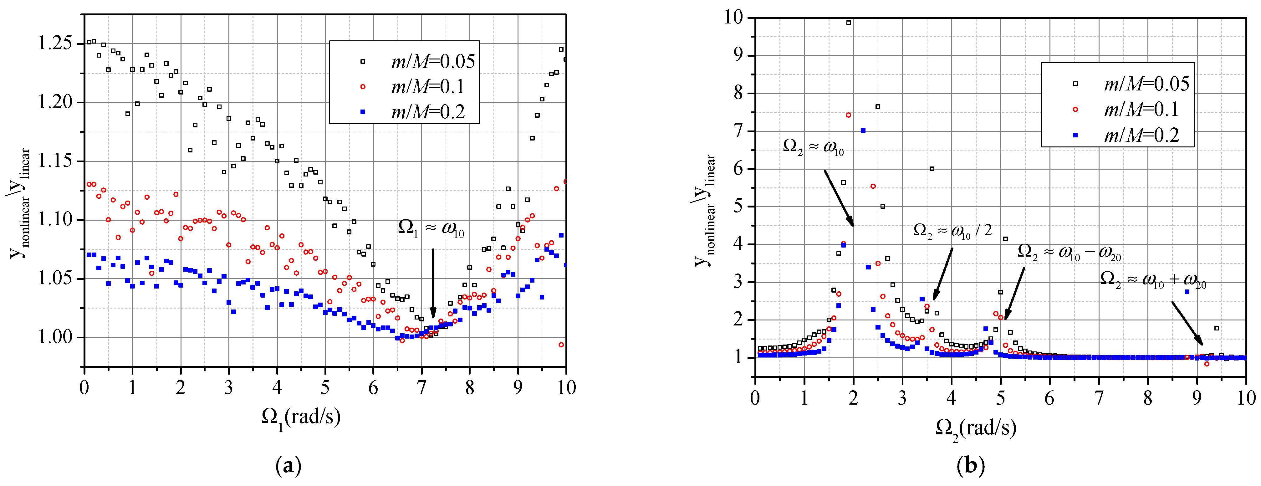
The structural frequency ratio is set to 0.3. As shown in Figure 8a, as excitation frequency to the primary structure approaches the primary resonant frequency, the nonlinear amplification coefficient gets close to 1.0, which exhibits weak nonlinearity of the primary structure; the primary structure shows a significant nonlinear effect as excitations deviate from the resonant frequency. Furthermore, the coefficient is larger at smaller mass ratios, which means that the structural nonlinear effect is strong at a small mass ratio. However, what is different is that the response of the primary structure is obviously amplified when the substructure is excited at not only the primary but also the secondary resonant frequencies, and that coefficients in some cases could reach up to three at the secondary resonance, as shown in Figure 8b. A nonlinear effect appears obvious when the substructure is excited at the secondary resonance.

5.2. Effect from Frequency Ratio

Amplification coefficients in different cases at distinct structural frequency ratios are given in four excitation combinations:

(1)

Low frequency excitation to the primary structure (Ω₁ = 0.1 rad/s), and low frequency excitation to the substructure (Ω₂ = 0.1 rad/s).

(2)

High frequency excitation to the primary structure (Ω₁ = 10 rad/s), and low frequency excitation to the substructure (Ω₂ = 0.1 rad/s).

(3)

Low frequency excitation to the primary structure (Ω₁ = 0.1 rad/s), and high frequency excitation to the substructure (Ω₂ = 10 rad/s).

(4)

High frequency excitation to the primary structure (Ω₁ = 10 rad/s), and high frequency excitation to the substructure (Ω₂ = 10 rad/s).

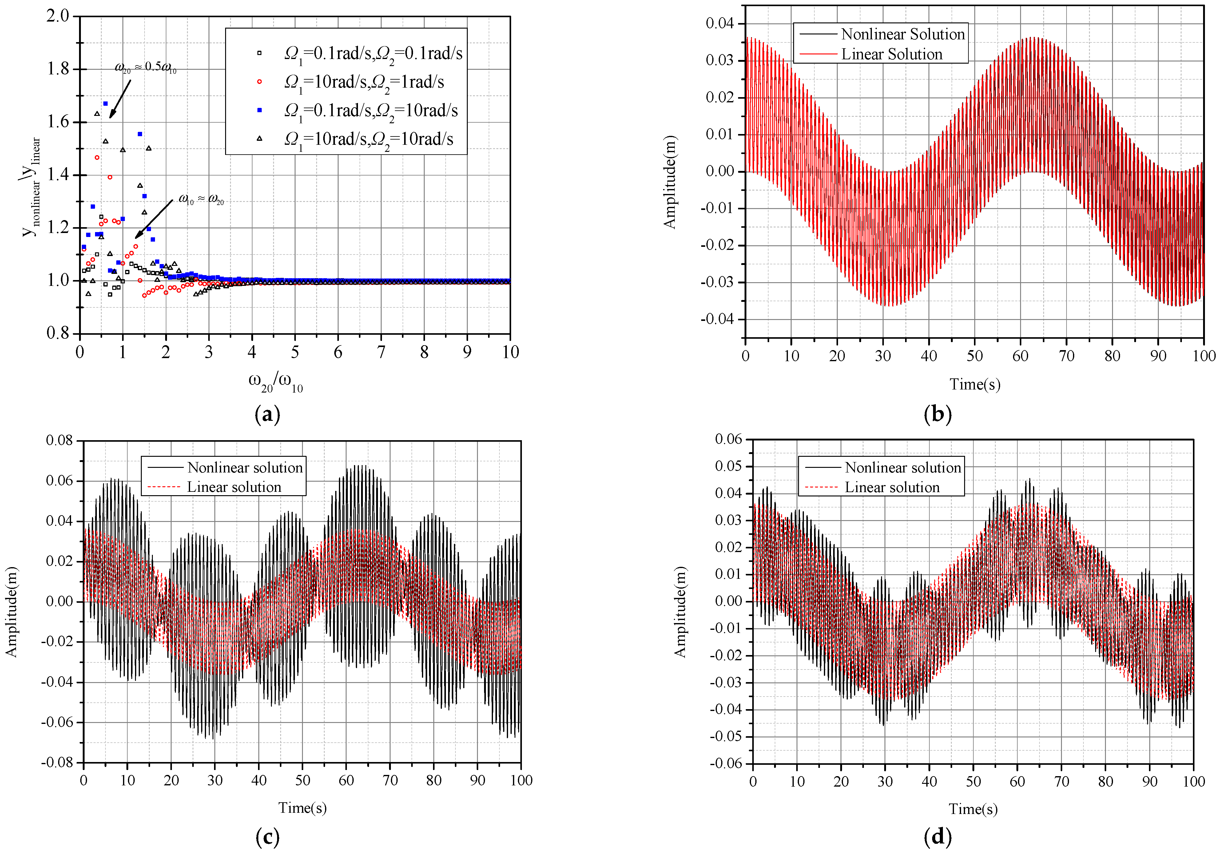
It is revealed in Figure 9a that amplification coefficients increase significantly to above 1.6 when the frequency ratio is around 0.5. It can be noticed that when the structural frequency ratio is near 1.0 and the substructure is excited at a low frequency, the response of the primary structure is also amplified, since it may cause the frequency (Ω₂ − ω₂₀ or Ω₂ + ω₂₀) of excitations to y₁ to approach the vertical frequency (ω₁₀), as referred to in Equation (15c).

As the frequency ratio exceeds 3.0, amplification coefficients tend to 1.0 gradually, which means that the nonlinear effect disappears at a high structural frequency ratio. In fact, as the frequency of the substructure gets higher, the connections between the primary structure and the substructure can be deemed stronger, and thus the substructure can be considered fixed to the primary structure to the extent that the nonlinear vibration is almost equivalent to the linear vibration. As shown in Figure 9b, when the structural frequency ratio reaches 10, the nonlinear time history curve almost coincides with the linear one.

When the frequency ratio is near 0.5, as shown in Figure 9c, the nonlinear vibration shows the “beat” oscillation along the specific path, which can explain the internal resonance in the free vibration, with the resonant vibration superimposed on the forced vibration.

It can be seen that when the frequency ratio reaches 1.0, a similar vibration with internal resonance occurs, and amplitude of the primary structure is augmented, as depicted in Figure 9d.

5.3. Effect from Relative Excitation

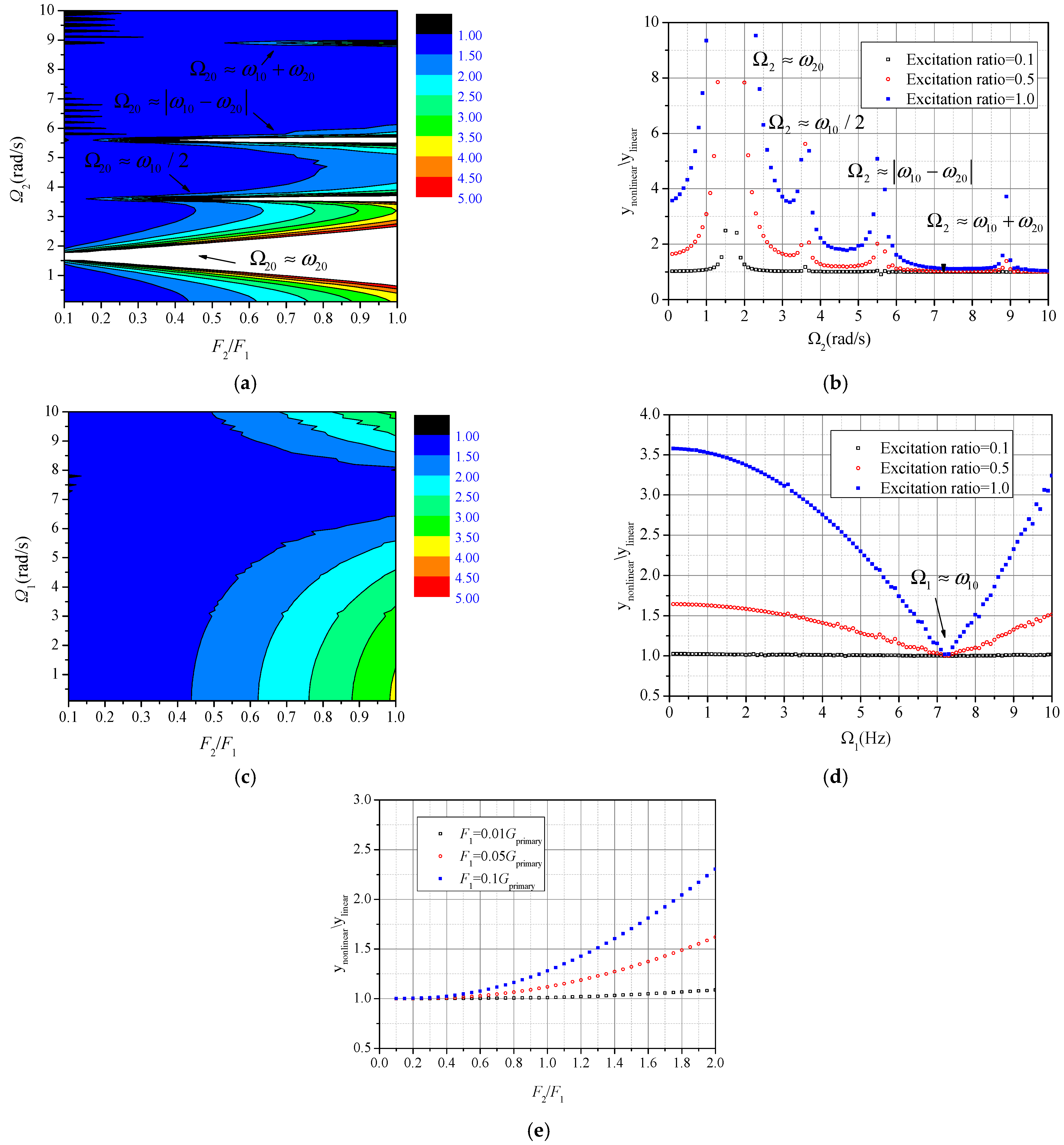
As mentioned above, excitation ratio and forcing amplitude are critical factors for the nonlinearity of the primary structure. Therefore, these two factors are analyzed parametrically at a mass ratio of 0.05 and a frequency ratio of 0.3. As depicted in Figure 10a,b, amplification of the primary structure becomes more severe as the excitation ratio increases from 0.1 to 1.0. Whenever the excitation frequency is around the primary or secondary resonant frequency, the nonlinearity of the primary structure appears significant. It can be found that excitations, when applied only to the primary structure, make the nonlinear effect negligible near the primary resonant frequency rather than at other frequencies, as displayed in Figure 10c,d.

Figure 10e illustrates the tendency of the amplification coefficients varying with the excitation ratio of distinct external forcing amplitudes of the primary structure, and the ratio of forcing amplitude to the gravity of the primary structure, which represents the relative force level, is discussed. It can be observed that when the forcing amplitude is about 0.01 times (1 percent) the gravity of the primary structure, the nonlinearity of the structure is not sensitive to the excitation ratio, and that the nonlinear effect grows rapidly with the excitation ratio when the force on the primary structure equals 0.1 times (10 percent) the gravity.

6. Case Study

In this section, a large-span roof structure with a suspended substructure is designed, and free and forced vibrations of the model are analyzed to validate the conclusions drawn above. ABAQUS/CAE (Version: 2020, ABAQUS Inc., Palo Alto, CA, USA) is adopted for the analysis.

6.1. Modeling

The primary structure is designed as a Kiewitte single-layer reticulated shell with a span of 30 m and a rise of 3 m. The diagram is shown in Figure 11a. The section of the dome member adopts steel pipes of φ 30 × 4. The live loads of about 0.08 kN/m are converted into nodal mass. There is a substructure suspended through the center of the dome structure by four hanging rods. The substructure consists of the rods and the beams. Sections of the rods are also pipes of φ 30 × 4, and a square section of 80 × 80 × 8 is adopted for the beams. The substructure is depicted in Figure 11b. Sliding bearings with constraints freedom released in a radial direction are set at the outer circle of the structure, as shown in Figure 11c.

The models with three distinct lengths of the rods are analyzed.

Table 3. Substructure parameters of different models.

Model	L (m)	f20 (Hz)	v0 (m)	θ0 (rad)	ω20 (rad/s)	ω20/ω10	m/M	Remarks
1	1	0.13	0.04	0.04	3.13	0.12	0.06	Hinged
2	2.5	2.06	0.1	0.04	12.93	0.5	0.06	Rigid
3	5	0.22	0.2	0.04	1.4	0.05	0.06	Hinged

displays specific parameters of two types of connections to the primary structure that are hinged and rigid. A diagram of the entire three-dimensional model is displayed in Figure 11d.

6.2. Modal Analysis

Modal and nonlinear time history analyses are conducted. The results of modal analysis are obtained to determine the vertical frequency of the dome structure (the primary structure) and the swing frequency of the substructure.

Modal information about model 2 is given in Figure 12, with the frequency of the vertical vibration being 3.98 Hz (ω₁₀ = 25.05 rad/s) and the swing frequency of the substructure being 2.03 Hz (ω₂₀ = 12.93 rad/s). It can be found that ω₂₀ ≈ 0.5ω₁₀, coinciding with the relation for internal resonance in Equation (11). Swing frequency information about the other models is listed in Table 2.

6.3. Nonlinear Analysis of Free Vibration

In the time history analysis, the distinct initial displacements listed in Table 2 are set up for the substructure at the same angle. As depicted in Figure 13, when initial lateral displacement of the substructure is 0.1 m, the corresponding angle is calculated to be about 0.04 rad. Geometric nonlinearity is considered in the analysis. The process of the analysis lasts for 20 s.

Time history vertical displacements of the dome at the monitoring point are illustrated in Figure 14. The results reveal that the structural frequency ratio of 0.5 contributes to the resonant vibration of the dome structure, which can be depicted as the “beat” oscillation, as shown in Figure 14a. Instead, dome structures of the other models continue vibrating at smaller amplitudes, as shown in Figure 14b. It can be demonstrated that the internal resonance has exactly amplified the response of the structure.

6.4. Nonlinear Analysis of Forced Vibration

Model 3 is taken for the forced vibration analysis. External forces applied to the substructure are shown in Figure 15. Three frequencies of excitations to the substructure are analyzed for the secondary resonance studied above. Information about excitation parameters is shown in

Table 4. Excitation parameters at different excitation frequencies.

Model	F2	Ω2 (rad/s)	Remarks
3-1	2000	12.12	Ω2 ≈ ω10/2
3-2	2000	22.84	Ω2 ≈ ω10 − ω20
3-3	2000	25.64	Ω2 ≈ ω10 + ω20

.

Figure 16a–c shows the vertical displacements at the monitoring point. According to these, when excitation frequencies reach the secondary resonant frequency, vertical displacements of the primary structure present the “beat” oscillation. As shown in Figure 16b,c, the time history curves are not standard for “beat” oscillation, probably because of the geometric nonlinearity of the structure such that the stiffness of the primary structure varies during vibration. In fact, the secondary resonance takes place exactly.

To sum up, the nonlinear vibration characteristics of the large-span suspended substructure deduced in Section 2 and Section 3 for the simplified model are demonstrated in the multiple-degrees-of-freedom system. Although vibration forms of the long-span suspended substructure are numerous and complicated, the vibration regulations obtained from the two-degrees-of-freedom model are proven valid, and these outcomes could guide the analysis of a multiple-degrees-of-freedom model when considering vertical vibration of the primary structure.

7. Conclusions

The large-span roof structure with a suspended structure has been investigated, nonlinear free and forced vibration equations for simplified models of the large-span structure with a suspended substructure have been set up, and nonlinear dynamic characteristics with different structural parameters have been explored by comparing linear and nonlinear results in this study. Conclusions can be drawn as follows:

(1)

Amplitude of the primary structure tends to be augmented at internal resonance if the structural frequency ratio nears 1:2. Vertical vibration of the primary structure and swing of the substructures could excite each other.

(2)

When frequencies at which excitations are applied to the substructure satisfy the conditions ${\mathrm{\Omega }}_2\approx {\omega }_{10}+{\omega }_{20}$, ${\mathrm{\Omega }}_2\approx \left|{\omega }_{20}-{\omega }_{10}\right|$ or ${\mathrm{\Omega }}_2\approx {\omega }_{10}/2$, amplitude of the primary structure may be augmented due to the secondary resonance.

(3)

A nonlinear effect on the structure is obvious as vertical excitations deviate from the vertical resonant frequencies, while excitations to the substructure gets close to the swing resonance. Frequency ratios and mass ratios have been identified as key factors for the primary structure’s nonlinearity, and the nonlinear effect appears weaker as mass ratios increase.

(4)

The substructure can be considered attached to the primary structure when connections between them are strong enough to reduce the nonlinear effect. The structure can be analyzed linearly for frequency ratios and mass ratios exceeding 3.0 and 0.1, respectively, according to the above studies.

(5)

In the design of this kind of structure, structural frequency ratios should be prevented from approaching 0.5, and external frequencies of ${\mathrm{\Omega }}_2\approx {\omega }_{10}+{\omega }_{20}$, ${\mathrm{\Omega }}_2\approx \left|{\omega }_{20}-{\omega }_{10}\right|$ or ${\mathrm{\Omega }}_2\approx {\omega }_{10}/2$ to the substructure should be taken into consideration as an additional check to ensure the safety of the structure.

These studies focusing especially on forced vibrations here are expected to lay a foundation for further ground motion analysis.