Article

Hesitant Fuzzy Linear Regression Model for Decision Making

1
Department of Statistics, Lahore Campus, COMSATS University Islamabad, Islamabad 45550, Pakistan
2
Research Team on Intelligent Decision Support Systems, Department of Artificial Intelligence and Applied Mathematics, Faculty of Computer Science and Information Technology, West Pomeranian University of Technology in Szczecin, ul. Żołnierska 49, 71-210 Szczecin, Poland
3
Department of Mathematics, Virtual University of Pakistan, Lahore 54000, Pakistan
*
Author to whom correspondence should be addressed.
Symmetry 2021, 13(10), 1846; https://doi.org/10.3390/sym13101846
Submission received: 1 August 2021 / Revised: 24 September 2021 / Accepted: 28 September 2021 / Published: 2 October 2021
(This article belongs to the Special Issue Uncertain Multi-Criteria Optimization Problems II)

Abstract

:
An expert may experience difficulties in decision making when evaluating alternatives through a single assessment value in a hesitant environment. A fuzzy linear regression model (FLRM) is used for decision-making purposes, but this model is entirely unreasonable in the presence of hesitant fuzzy information. In order to overcome this issue, in this paper, we define a hesitant fuzzy linear regression model (HFLRM) to account for multicriteria decision-making (MCDM) problems in a hesitant environment. The HFLRM provides an alternative approach to statistical regression for modelling situations where input–output variables are observed as hesitant fuzzy elements (HFEs). The parameters of HFLRM are symmetric triangular fuzzy numbers (STFNs) estimated through solving the linear programming (LP) model. An application example is presented to measure the effectiveness and significance of our proposed methodology by solving a MCDM problem. Moreover, the results obtained employing HFLRM are compared with the MCDM tool called technique for order preference by similarity to ideal solution (TOPSIS). Finally, Spearman’s rank correlation test is used to measure the significance for two sets of ranking.

1. Introduction

The fuzzy set theory introduced by Zadeh [1] provides an excellent base to work in uncertain and ambiguous situations with incomplete information. The fuzzy set theory has been applied in different research areas to handle uncertainty, such as medical and life sciences [2,3], management sciences [4,5], social sciences [6], engineering [7], statistics, artificial intelligence [8], robotics, computer networks, and decision making [8,9,10,11,12]. As an important extension of fuzzy set theory, Torra [13] introduced a hesitant fuzzy set (HFS) which allows a set of possible values and takes the degrees of membership it can express the hesitant information more comprehensively. HFS attracted many researchers in a short period because of its frequent usage in hesitant situations in real-world problems. Recently, many researchers have shown great attention to work with the decision-making problems in the framework of hesitant fuzzy information [14]. For example, Mardani et al. [15] proposed an extended approach under HFSs for assessing the key challenges of digital health intervention adoption during the COVID-19 pandemic, Narayanamoorthy et al. [16] suggested an approach for the site selection of underground hydrogen storage based on normal wiggly dual HFSs, Dong and Ma [17] developed an enhanced fuzzy time series model based on hesitant differential fuzzy sets and error learning, and so on.
It is a tedious process to seek out the most straightforward alternative among the available choices. An outsized number of techniques are being used to facilitate the decision makers (DMs) for ranking alternatives in decision-making problems. Since 1960, MCDM has been an active research area, and there are several methods that DMs frequently use for decision making such as TOPSIS [18], Best Worth Method [19] (and its extension [20]), Evaluation based on Distance from the Average Solution [21], and so on. In the current era, several professionals have employed MCDM methods and strategies to deal with the problems of the modern age. For example, Wang et al. [22] proposed a three-way decision method for MCDM problems based on hesitant fuzzy information, and Farhadinia and Herrera-Viedma [23] proposed several new forms of distance and similarity measures and an extended TOPSIS method for dealing with MCDM problems in the context of dual HFS.
For several years, regression analysis has been used to determine the relationship between the output variable (dependent variable) and one or more than one input variable (independent variables). Traditionally, regression modelling examined crisp data and relationships; however, we can assume a fuzzy relationship between an output variable and input variables is more practical if the phenomenon under study is imprecise. Initially, a possibilistic approach for fuzzy regression analysis was proposed by Tanaka et al. [24]. They introduced a linear system for solving the FLRM. Further, Tanaka [25] improved the possibilistic approach and introduced fuzzy interval analysis in which possibilistic linear models were proposed with non-fuzzy inputs and fuzzy outputs. These approaches were criticized due to having non-interactive possibilistic parameters by Celmins [26] who described the fuzzy least square method as a fuzzy vector and also illustrated the least square fitting for fuzzy models when data are available in n-component vectors. Diamond [27] introduced fuzzy least square models as well as normal equations that are similar to classical least squares. Tanaka and Watada [28] developed linear programming using possibilistic measures and estimated the parameters of the FLRM.
To answer the criticism about non-interactive possibilistic parameters, Tanaka and Ishibuchi [29] presented an identification method for the interactive fuzzy parameters in which they used quadratic membership functions in the possibilistic linear systems. Sakawa and Yano [30] developed a group of FLRMs that use indices about the equality of two fuzzy numbers. Peters [31] elaborated a general form of Tanaka’s approach [24] into fuzzy intervals with fuzzy linear programming. Kim and Chen [32] presented comprehensive research between non-parametric linear regression and FLRMs. Yen et al. [33] improved the fuzzy regression model with symmetric triangular parameters. This approach helped in reducing inflexibility, which was present in the earlier developed models. Chen [34] presented a study to handle the outliers in a case when data are available in the form of non-fuzzy input and fuzzy output with some more constraints so that the effect of outliers can be reduced. Kocadagli [35] addressed the problem of the h-cut level with a constrained non-linear programming method and developed effective solutions for fuzzy regression. Choi and Buckley [36] proposed a fuzzy least absolute approach to estimate the fuzzy parameters and to examine the performance of fuzzy regression models with the help of specific error measures. Recently, Cerny and Rada [37] derived a possibilistic generalization technique for the linear regression model using censored/rounded data. In decision making for robot selection, Karsak et al. [38] used a FLRM for alternatives ranking in the robot selection. Several issues concerning fuzzy regression analysis have been discussed in recent years. For example, Icen and Dermirhan [39] used a Monte Carlo simulation to the error measurements in the FLRM, Choi et al. [40] determined an algorithm to address the problem of multicollinearity by combining the approaches of ridge regression and fuzzy regression model, Chakravarty et al. [41] proposed robust fuzzy regression functions based on fuzzy k-means clusters against the outliers, Wang et al. [42] helped in the approximation Bayesian computation of FLRM and used a likelihood-free function for generating samples from the posterior distribution, Hesamian and Akbari [43] proposed a fuzzy additive regression model using kernel smoothing for estimating a fuzzy smooth function, and Boukezzoula and Coquin [44] redefined interval-valued type-1 and type-2 fuzzy regression models in terms of philosophy and methodology.
From the above literature review, we can see the work performed in the field of fuzzy regression analysis over the last few decades and how gradually this field has evolved and is still evolving. We found from the research examined that most of the work has been performed using FLRM. However, the FLRM does not address the situations where input variables and output variables are observed in a hesitant environment. This paper thus extends the work [31] in a hesitant environment and observes input–output variables as HFEs. We introduce the concept of HFLRM such that the coefficients of the model are STFNs. Practically, we have used this model to facilitate an organization in generating revenue, and several variables (goods and services) are taken into account when calculating revenue generation. A large organization contains many experts and wishes to utilize their expertise in their respective fields to come to a more plausible decision. Therefore, experts may advise different values (between 0 and 1) when analyzing certain variables. For example, one expert may suggest 0.2, the second may suggest 0.4, and the third 0.5, which can be represented by an HFE such as 0.2, 0.4, 0.5, which is the basic form of the HFS. Thus, motivated by HFS, the HFLRM incorporates these HFEs into the regression analysis and estimates the HFLRM parameters using the LP model. Furthermore, the alternatives are ranked using the residual values of the proposed HFLRM. To validate the proposed method, the HFLRM findings are compared to those of the most widely used MCDM technique, TOPSIS.
This paper is organized as follows: Section 2 defines some preliminary concepts related to the research work. Section 3 presents the idea of HFLRM and then proposes a decision-making algorithm with HFLRM in the framework of a hesitant environment. In Section 4, we present the TOPSIS method and Spearman rank correlation test and some popular similarity coefficients. An application example using the proposed HFLRM is presented in Section 5. Results and discussions are provided in Section 6. Finally, concluding remarks are given in Section 7.

2. Preliminaries

This section introduces the basic knowledge that is necessary to understand the proposed study.
Torra [13] defined HFS in terms of a function that returns a set of membership values for each element in the domain as follows:
Definition 1
([45]). Let Z be a reference set, a HFS A on Z in terms of a function h ( z ) that when applied to Z returns a finite subset of [ 0 , 1 ] , which can be represented as the following mathematical symbol:
A = z , h ( z ) z | z Z
where h ( z ) is a set of some values in [ 0 , 1 ] , denoting the hesitant membership degrees of the element z Z to the set A. For convenience, h ( z ) or simply h, is called a hesitant fuzzy element (HFE).
Example 1.
If Z = { z 1 , z 2 , z 3 } is the reference set, h ( z 1 ) = { 0.4 , 0.5 , 0.6 } , h ( z 2 ) = { 0.1 , 0.2 , 0.3 } and h ( z 3 ) = { 0.7 , 0.8 } are the possible membership degrees of z i ( i = 1 , 2 , 3 ) to a set A, respectively. Then the HFS A can be represented as follows:
A = { z 1 , { 0.4 , 0.5 , 0.6 } , z 2 , { 0.1 , 0.2 , 0.3 } , z 3 , { 0.7 , 0.8 } } .
Definition 2
([46]). Let h be a HFE as mentioned above. The score function of h can be defined as:
S c ( h ) = 1 # ( h ) γ h γ
For two HFEs h 1 and h 2 , if S c ( h 1 ) > S c ( h 2 ) , then h 2 h 1 , if S c ( h 1 ) = S c ( h 2 ) , then h 1 h 2 .
Definition 3
([47]). Let h , h 1 , and h 2 be three HFEs, then the following operational laws always hold for λ > 0 .
1 . h λ = γ h γ λ ; 2 . λ h = γ h 1 1 γ λ ; 3 . h 1 h 2 = γ 1 h 1 , γ 2 h 2 { γ 1 γ 2 } ; 4 . h 1 h 2 = γ 1 h 1 , γ 2 h 2 { γ 1 + γ 2 γ 1 γ 2 } .
Definition 4
([48]). The membership function for a fuzzy number, F n is as follows:
μ F n z = L t m z c L t , z m , c L t 0 R t z m c R t , z m , c R t 0
where z R , L t and R t are left and right reference functions of the membership function, respectively. The c L t and c R t are the left and right spreads, respectively, and m is the mode of the fuzzy number. The distance from the left end-point to the mode and the distance from mode to the right end-point is represented by c L t and c R t , respectively. A special form of L t and R t type fuzzy number is known as the triangular fuzzy number (TFN) when its membership function has the following form.
Definition 5
([48]). The TFN denoted by ( a , m , b ) can be defined as:
μ t z ; a , m , b = 1 m z m a , a z m , 1 z m b m , m < z b , 0 , elsewhere .
Moreover, if c L t = c R t then the TFN is known as a symmetrical triangular fuzzy number (STFN). Some particular fuzzy arithmetic that is used in this study is described as follows:
Definition 6
([48]). Suppose, F n 1 = ( a 1 , m 1 , b 1 ) and F n 2 = ( a 2 , m 2 , b 2 ) are two TFNs; addition, subtraction, and scalar multiplication of TFNs are defined as:
F n 1 + F n 2 = a 1 + a 2 , m 1 + m 2 , b 1 + b 2 F n 1 F n 2 = a 1 a 2 , m 1 m 2 , b 1 b 2 s F n 1 = ( s a 1 , s m 1 , s b 1 ) , s 0

3. Decision Making Based on Hesitant Fuzzy Linear Regression Model

In this section, we define the concept of HFLRM from the statistical point of view on the basis of hesitant fuzzy information. However, before this, it is necessary to provide a brief review of existing regression models which are available in the literature.

3.1. Linear Regression Model

A multiple linear regression model with output variable Y i ( i = 1 , 2 , 3 , , M ) and the input variables X 1 , , X N is defined as
Y i = A 0 + A 1 X i 1 + A 2 X i 2 + A 3 X i 3 + + A N X i N + ε i ,
where parameters A 0 , A 1 , , A N are crisp numbers, and ε i is the random error of the model. In the linear regression model, errors are assumed normally distributed with zero mean and constant variance.

3.2. Fuzzy Linear Regression Model

Tanaka et al. [24] proposed FLRM, which measures the relationship between the variables where the relationship among the variables is vague and regression residuals (the difference between observed and predicted values) are assumed to be due to the imprecise nature of the system. The FLRM model is defined as:
Y ^ i = A ˜ 0 + A ˜ 1 X i 1 + A ˜ 2 X i 2 + A ˜ 3 X i 3 + + A ˜ N X i N ,
where fuzzy parameters A ˜ j = ( α j , c j ) are STFNs, and α j and c j represent center and spread of STFNs, respectively. The FLRM addresses the problem of the determination of fuzzy parameter estimates A ˜ j such that the membership value of Y i to its fuzzy estimate Y ^ i is at least H, where H [ 0 , 1 ) , also known as a measure of the goodness-of-fit, is provided by the decision maker [49]. The objective of the FLRM is to minimize the uncertainty by minimizing the spreads of the fuzzy numbers. This problem leads to following LP model [28]:
min j = 0 N c j i = 0 M x i j
subject to the constraints
j = 0 N α j x i j + L 1 ( H ) j = 0 N c j x i j y i , j = 0 N α j x i j L 1 ( H ) j = 0 N c j x i j y i , x i 0 = 1 , c j 0
where L is the membership function of a standardized fuzzy parameter [38].
Peters [31] modified Tanak’s model by compensating good and bad data (outliers) within estimated intervals as it was not able to handle bad data. Peters [31] introduced a new variable λ (a membership degree which conforms to a set of good solutions) and used arithmetic mean [50] as the aggregation operator. It is defined as:
max λ ¯ = 1 M i = 1 M λ i
subject to the constraints
1 λ ¯ p 0 i = 0 M j = 0 N c j x i j d 0 , 1 λ i p i + j = 0 N α j x i j + j = 0 N c j x i j y i , 1 λ i p i j = 0 N α j x i j + j = 0 N c j x i j y i , L 1 ( H ) = 1 , 0 λ i 1 , x i 0 = 1 , c j 0 ,
The width of the estimated interval depends on the selection of the parameters d 0 , p 0 , p i which are chosen according to the nature of problem. The parameter p i represents the width of the tolerance interval of the output variable. A permissive condition for spread minimization leads in a wide interval, i.e., a large value of p 0 and a small value of p i . On the other hand, strict conditions for minimizing the spread results in a small interval, i.e., a small p 0 and a large p i . The parameter d 0 represents the desired value of an objective function. Since the purpose of FLRM is to minimize the total spread, it is suggested that parameter d 0 is selected as 0 (Peters [31]).

3.3. Hesitant Fuzzy Linear Regression Model

Motivated by Peters’ model [31], we propose the concept of HFLRM which can be used further in solving the decision-making problems. We will take the output variable Y i ( i = 1 , 2 , , M ) and the input variables X j ( j = 0 , 1 , 2 , , N ) as HFEs. The HFLRM is defined as:
Y i = β ˜ 0 X 0 β ˜ 1 X 1 β ˜ 2 X 2 β ˜ 3 X 3 β ˜ N X N
where, Y i = { y i k | 1 < i < M , 1 < k < P } and X j = { x i j k | 1 < i < M , 0 < j < N , 1 < k < P } . The parameters β ˜ j = α j k , c j k , 0 < j < N and 1 < k < P are STFNs which are estimated with the help of the following LP model:
max λ k ¯ = 1 M i = 1 M λ i k
subject to the constraints
1 λ k ¯ p 0 i = 1 M j = 0 N c j k x i j k d 0 , 1 λ i k p i + j = 0 N α j k x i j k + j = 0 N c j k x i j k y i k , 1 λ i k p i j = 0 N α j k x i j k + j = 0 N c j k x i j k y i k , λ i k 1 , x i 0 k = 1 , c j k 0 .
where k determines several values assigned by P DMs for the output variable Y i and input variables X j .

3.4. Decision-Making Algorithm Based on HFLRM

Assume that A = { A 1 , A 2 , , A M } is a set of alternatives and D = { d l , 1 < l < P } is a set of DMs who provide their evaluations in the form of HFEs about alternatives A i under some input variables X j ( j = 0 , 1 , 2 , , N ) and output variable Y i   ( i = 1 , 2 , , M ) . Let H 1 = [ X i j ] M × N be an input variable decision matrix, and H 2 = [ Y i ] M × 1 be an output variable decision matrix, where X i j = { x i j k , k = 1 , 2 , , # ( X i j ) } and Y i = { y i k , k = 1 , 2 , , # ( Y i ) } are HFEs.
Step 1. 
Let H = [ Z i j ] M × ( N + 1 ) be a connected input–output variable decision matrix provided by the DMs, where Z i j = { z i j k , k = 1 , 2 , , # ( Z i j ) } are HFEs.
Step 2. 
For two finite HFEs, h 1 and h 2 , there are two opposite principles for normalization. The first one is α -normalization in which we remove some elements of h 1 and h 2 which have more elements than the others. The second one is β -normalization in which we add some elements to h 1 and h 2 which have fewer elements than the other. In this paper, we use the principle of β -normalization [51] to make all HFEs equal in the matrix H. Let H ¯ = [ Z ¯ i j ] M × ( N + 1 ) be the normalized matrix where Z ¯ i j = { z ¯ i j k , k = 1 , 2 , , P } are HFEs.
Step 3. 
Again normalize the matrix H ¯ by using the following equation:
Z ^ i j = z ¯ i j k min ( Z ¯ i j ) max ( Z ¯ i j ) min ( Z ¯ i j )
Let H ^ = [ Z ^ i j ] M × ( N + 1 ) be a normalized decision matrix where Z ^ i j = { z ^ i j k , k = 1 , 2 , , P } are HFEs.
Step 4. 
By estimating the parameters with the help of a linear programming model, the HFLRM is obtained using the normalized decision matrix H ^ .
Step 5. 
Rank the alternatives using residual values obtained from the score values of Y i ( i = 1 , 2 , , M ) and Y i ( i = 1 , 2 , , M ) , i.e., e i = S c ( Y i ) S c ( Y i ) , where Y i are predicted values which are calculated by using Definitions 2, 3 and 6.
Step 6. 
Finally, the alternatives are ranked according to the values of e i ( i = 1 , 2 , , M ) . The alternative with the least residual is identified as the best choice.
A multiple linear regression model (Section 3.1) is a very effective and reliable technique for determining the effect of one or more input variables on an output variable. It is the most extensively used statistical technique and has a wide variety of practical applications. It is based on precise data and a precise relationship between the output variables and input variables. However, despite the widespread use of the model (Section 3.1) in everyday activities, there exists uncertainty in variables. In real life, there are several situations in which data are not provided as a precise quantity but rather as incomplete, ambiguous, linguistically imperfect, and imprecise. The FLRM (Section 3.2) was introduced to deal with such uncertainty and ambiguity. Recently, many researchers have presented statistical regression analysis in the framework of fuzzy set theory. The HFS is an extension of fuzzy set theory that has drawn the attention of many researchers in a short period because we can observe hesitation in a variety of real-world scenarios, and this novel technique helps us deal with the ambiguity caused by hesitation. This is why we have extended the idea of FLRM (Section 3.2) to HFLRM (Section 3.3) where input–output variables are observed as HFEs, which is a basic form of HFS.

4. The TOPSIS Method under Hesitant Environment

Hwang and Yoon [18] developed an MCDM technique, TOPSIS, which is based on the belief that the alternative solution that is selected (solution) should have the shortest distance to the ideal solution (alternative) and the farthest distance from the negative ideal solution for all the available alternatives [52]. When criteria values are HFEs then the mathematical formulation of the TOPSIS method will be as follows:
Step 1. 
Take the decision matrices H and H ¯ , the same as mentioned in Steps 1 and 2 of Section 3.4.
Step 2. 
Normalize the decision matrix H ¯ with the help of the following formula:
Z ^ i j = z ¯ i j k z ¯ i j k 2
Let H ^ = [ Z ^ i j ] M × ( N + 1 ) be the normalized decision matrix where, Z ^ i j = { z ^ i j k , k = 1 , 2 , , P } are HFEs.
Step 3. 
Weighted normalized decision matrix is calculated by multiplying the normalized decision matrix with its associated weights, i.e., V i j = Z ^ i j × W j .
Step 4. 
Determine the positive ideal solution A + and negative ideal solution A
A + = { ( max i V i j | j J b ) , ( min i V i j | j J c | i = 1 , 2 , , N ) } = { A 1 + , A 2 + , , A J + , , A N + 1 } A = { ( max i V i j | j J b ) , ( min i V i j | j J c | i = 1 , 2 , , N ) } = { A 1 , A 2 , , A J , , A N + 1 }
where J b and J c represent the set of benefit and cost criteria, respectively.
Step 5. 
Calculate the Euclidean distance of each alternative A i from the positive ideal solution A + and negative ideal solution A , respectively.
D i + = j = 1 N + 1 V i j A j + 2 D i = j = 1 N + 1 V i j A j 2 where i = 1 , 2 , , M .
Step 6. 
Calculate the relative closeness P i of each alternative to the ideal solution where
P i = D i D i + D i + , i = 1 , 2 , , M .
Step 7. 
Rank the alternatives A i ( i = 1 , 2 , , M ) according to relative closeness values P i in the descending order.

Spearman’s Rank Correlation Coefficient

Spearman’s rank correlation is a method for analyzing the relationship between ordinal measurement level variables. It is high when observations have a similar rank and low when observations have a different rank between the two sets of values. Spearman’s rank correlation coefficient, r s , is defined as follows:
r s = 1 6 d 2 M 2 M 1
where d i = R i 1 R i 2 is the ranking difference while R i 1 and R i 2 indicate the two sets of ranking. The rank correlation coefficient ranges from + 1 to 1 . The r s = ± 1 indicates a perfect positive ( r s = + 1 ) and perfect negative ( r s = 1 ) relationship between the two sets of ranking.
We often want to know whether or not a significant relationship exists between two sets of ranking. Therefore, we state the null hypothesis ( H 0 ) and alternative hypothesis ( H 1 ) as:
H 0 : There is no significant relationship between the two sets of ranking.
H 1 : There is a significant relationship between the two sets of ranking.
The null hypothesis is evaluated using the following test statistic provided that the sample size is not too small, i.e., M > 10 .
Z c = r s M 1
If the Z c statistic value exceeds the critical value Z α (usually, α = 0.05 ), then the null hypothesis is rejected, and we conclude that there is a significant relationship between the two sets of ranking.

5. An Application Example

Revenue is essential for nearly every structure of organization. Any organization must generate revenue in order to cover the gross and net operating costs. The owner of a well-known business chain wants to determine which outlet made the most revenue throughout the month of holy Ramadan. The revenue generated by a store is determined by the sale of goods ( X 1 ) , production expenditures ( X 2 ) , operational costs ( X 3 ) , and the profit margin ( Y ) . In this study, 20 store outlets A i ( i = 1 , 2 , , 20 ) are given in the form of alternatives. These alternatives are evaluated by the output variable Y i ( i = 1 , 2 , , 20 ) and input variables X j + 1 ( j = 0 , 1 , 2 ) . Three experts/DMs from senior management have made their judgements on the input and output variables. The solution to the given problem comprises the following steps:
Step 1. 
The connected input–output variable decision matrix provided by the DMs by using HFEs is shown in Table 1.
Step 2. 
To make all HFEs equal in the decision matrix H, we use the principle of β -normalization and obtained matrix H ¯ which can be seen in Table 2.
Step 3. 
We further normalize the data of matrix H ¯ to make all of its elements lie between 0 and 1 for a common scale. The normalized decision matrix H ^ is shown in Table 3.
Step 4. 
Now, we estimate the parameters using the LP model by taking d 0 = 0 , p 0 = 1000 and p i = 1 , which is formulated as follows:
For k = 1
M a x λ 1 ¯ = i = 1 M λ i 1 M
Subject to the constraints
λ 1 1 + λ 2 1 + . . + λ 20 1 + 20 1000 20 c 0 1 + 18.2893 c 1 1 + 11.2411 c 2 1 + 0.409 c 3 1 20
and
λ 1 1 α 0 1 + 0.8434 α 1 1 + 0.5783 α 2 1 + 0.0361 α 3 1 c 0 1 + 0.8434 c 1 1 + 0.5783 c 2 1 + 0.0361 c 3 1 0 λ 2 1 α 0 1 + 0.9036 α 1 1 + 0.5663 α 2 1 + 0.0241 α 3 1 c 0 1 + 0.9036 c 1 1 + 0.5663 c 2 1 + 0.0241 c 3 1 0.988 λ 3 1 α 0 1 + 0.9518 α 1 1 + 0.5542 α 2 1 + 0.0120 α 3 1 c 0 1 + 0.9518 c 1 1 + 0.5542 c 2 1 + 0.0120 c 3 1 0.9639 λ 20 1 α 0 1 + 0.8795 α 1 1 + 0.5783 α 2 1 + 0.0361 α 3 1 c 0 1 + 0.8795 c 1 1 + 0.5783 c 2 1 + 0.0361 c 3 1 0
λ 1 1 + α 0 1 + 0.8434 α 1 1 + 0.5783 α 2 1 + 0.0361 α 3 1 c 0 1 + 0.8434 c 1 1 + 0.5783 c 2 1 + 0.0361 c 3 1 1 λ 2 1 + α 0 1 + 0.9036 α 1 1 + 0.5663 α 2 1 + 0.0241 α 3 1 c 0 1 + 0.9036 c 1 1 + 0.5663 c 2 1 + 0.0241 c 3 1 1.012 λ 3 1 + α 0 1 + 0.9518 α 1 1 + 0.5542 α 2 1 + 0.0120 α 3 1 c 0 1 + 0.9518 c 1 1 + 0.5542 c 2 1 + 0.0120 c 3 1 1.0361 λ 20 1 + α 0 1 + 0.8795 α 1 1 + 0.5783 α 2 1 + 0.0361 α 3 1 c 0 1 + 0.8795 c 1 1 + 0.5783 c 2 1 + 0.0361 c 3 1 1
After solving the LP model as mentioned above, we get the values of λ i 1 ( i = 1 , 2 , , 20 ) , α j 1 ( j = 1 , 2 , 3 , 4 ) , and c j 1 ( j = 1 , 2 , 3 , 4 ) for k = 1 , which are shown in Table 4. In the same way, we can also obtain the results for k = 2 and k = 3 which are given in the same table.
We can see in Table 4 that the estimated values λ i k obtained through solving a LP model are either equal to 1 or very close to 1. It indicates that there is no outlier present in the given data. Now, the fuzzy linear regression models for k = 1 , 2 , 3 are given as follows:
y 1 = ( 0.05474 , 0 ) + ( 0.1548 , 0.005296 ) x 1 1 + ( 0.1049 , 0 ) x 2 1 + ( 0.4456 , 0.108200 ) x 3 1
y 2 = ( 0.35570 , 0 ) + ( 0.2530 , 0.004056 ) x 1 2 + ( 0.001166 , 0 ) x 2 2 + ( 0.5682 , 0.004408 ) x 3 2
y 3 = ( 0.2978 , 0.0006209 ) + ( 0.2301 , 0 ) x 1 3 + ( 0.2282 , 2.5294 e 12 ) x 2 3 + ( 0.6463 , 0.1822 ) x 3 3
Finally, the resultant estimated HFLRM in this case is given as
Y = ( 0.2360 , 0.0002070 ) ( 0.2126 , 0.003117 ) X 1 ( 0.1355 , 8.4316 e 13 ) X 2 ( 0.5534 , 0.09827 ) X 3 .
Steps 5 and 6. 
Now, we will find the estimated values of all the alternatives in the form of HFEs with the help of HFLRM Y . For the sake of paper length, we omit the calculation of the estimated values of all alternatives and keep ourselves fixed to calculate the estimated value of the first alternative A 1 only. By using Definitions 3 and 6, the HFE Y 1 corresponding to first alternative A 1 is computed as follows:
Y 1 = { 0.2437, 0.2564, 0.2701, 0.2452, 0.2579, 0.2715, 0.2467, 0.2594, 0.2730, 0.2412, 0.2539, 0.2677, 0.2427, 0.2554, 0.2691, 0.2442, 0.2569, 0.2705, 0.2387, 0.2515, 0.2652, 0.2401, 0.2529, 0.2667, 0.2417, 0.2544, 0.2681}
The score value of Y 1 is then calculated by using Definition 2 which is S c ( Y 1 ) = 0.2557 . Similarly, we can find the score values of all Y i ( i = 2 , , 20 ) which can be seen in Table 5. Finally, the alternatives are ranked with the help of residual values e i = S c ( Y i ) S c ( Y i ) , i = 1 , 2 , , 20 , where S c ( Y i ) ( i = 1 , 2 , , 20 ) are score values of HFEs corresponding to all alternatives in Table 1. The final ranking order of alternatives is shown in Table 5. We can see outlet 9 has the smallest residual value, i.e., e 9 = 0.8119 while outlet 12 has the largest residual value, i.e., e 12 = 0.2452 . Therefore, A 9 is considered the best alternative and the worst alternative is A 12 .

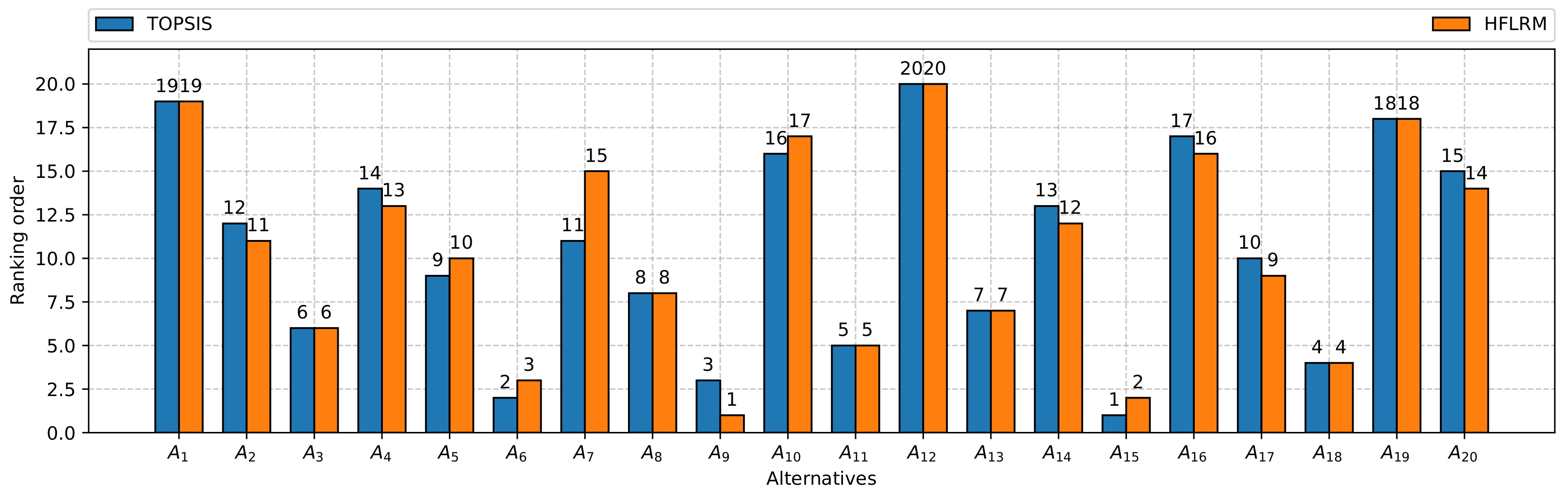
6. Results and Discussion

To check the validity and feasibility of our proposed approach, a MCDM tool called the TOPSIS method is applied to solve the same problem and we compare the results of the proposed approach with the results obtained in the TOPSIS method. Among the four criteria, we take the sale of goods ( X 1 ) and the profit margin ( Y ) as benefit criteria, while production expenditures ( X 2 ) and operational costs ( X 3 ) are considered cost criteria. After normalizing the matrix H ¯ according to step 2 of the TOPSIS algorithm, the PIS ( A + ) and NIS ( A ) are as follows:
A + = { { 0.243288 , 0.24311 , 0.243275 } , { 0.238388 , 0.238494 , 0.236583 } , { 0.217587 , 0.217382 , 0.217604 } , { 0.200482 , 0.201767 , 0.202947 } } A = { { 0.20274 , 0.20369 , 0.204863 } , { 0.208896 , 0.209291 , 0.207614 } , { 0.228466 , 0.228161 , 0.228306 } , { 0.240578 , 0.240819 , 0.240999 } }
Now we calculate the Euclidean distances D i + and D i of each alternative A i from A + and A along with its relative closeness P i to the ideal solution by using Step 5 and Step 6 of Section 4. The values of D i + , D i , P i and the ranking of alternatives ( R T o p s i s ) can be seen in Table 6.
In Table 6, we can see alternative 15, with the largest value of P i , is the best alternative, while alternative 12, with the smallest value of P i , is generating the lowest revenue among the stores. Additionally, we have compared the two sets of ranking R H F L R and R T o p s i s through a bar chart given in Figure 1.
Figure 1 illustrates a visual representation of the alternative ranking approach using the HFLRM and TOPSIS methods. We can see outlet number 9 is at the top of the list for generating the most revenue employing HFLRM during the holy month of Ramadan, and it is also the third best earning outlet according to the TOPSIS technique. Similarly, store 15 generates the second highest revenue when HFLRM is used and the highest revenue when TOPSIS is used. Likewise, all other outlets have the same ranking or very similar ranking for both HFLRM and TOPSIS.
Whereas the graphical representation provides a quick summary of the performance of two ranking sets R H F L R and R T o p s i s , it is not conclusive. As a result, the Spearman rank correlation coefficient is calculated to determine the statistical significance of the two sets of ranking, as shown in Table 7.
The Spearman rank correlation coefficient is calculated as r s = 1 6 ( 30 ) 7600 = 0.98 .
The coefficient r s = 0.98 is close to + 1 in Table 8, indicating that there is a very strong positive correlation between two sets of ranking, R H F L R and R T o p s i s . In order to evaluate whether the result is meaningful or merely down to chance, we performed a test of the null hypothesis that there is no very strong positive relationship between two sets of ranking, versus the alternative that there is a very strong positive relationship between two sets of ranking at a 5 % level of significance. The value of test statistics, Z c = r s M 1 = 0.97 20 1 = 4.22 falls within the critical region, Z 0.05 = 1.645 (derived from the statistical table of cumulative normal distribution); therefore, our null hypothesis would be rejected. We conclude that there is a very strong positive correlation between the two sets of ranking. In addition, we determined the values of the similarity coefficients of the two final rankings using r w and W S , which are described more extensively in [53,54]. The value of the weighted Spearman coefficient was 0.9781, and for the weighted similarity, the value was 0.9258. Thus, both coefficients determine a very strong relationship between the two final rankings. In addition, the proposed approach has the following advantages over the TOPSIS method:
  • The HFLRM can identify outliers (i.e., λ i ) that may be included in the data set; if these are not identified, it may result in an inaccurate solution. However, the data presented in the application example of this paper have no outlier.
  • The HFLRM provides results by solving a simple LP model to obtain the ranking for the decision-making problem which provides results quickly with less computational time as compared to TOPSIS.
  • In comparison with TOPSIS, the complexity of the proposed methodology does not increase by inserting more criteria and alternatives to the given MCDM problem.

7. Conclusions

This paper provides a multi-criteria decision-making approach for fuzzy linear regression models that incorporates hesitant information. This concept has not been explored previously and is a novel alternative to statistical regression in resolving MCDM challenges. We have implemented our proposed methodology to choose the best store outlet for the most revenue in a certain month. We have evaluated 20 alternative store outlets nationwide in the context of four criteria that have a major impact on the revenue generation for a chain of stores. Similarly, we may include more criteria and alternatives, but computing becomes more complicated as the number of alternatives or criteria examined increases. Finally, the suggested methodology’s outcomes are compared to those of a widely used decision-making technique, TOPSIS. In the future, we will further investigate the applications of HFLRM in decision making with hesitant fuzzy linguistic term sets and the probabilistic hesitant fuzzy linguistic sets.

Author Contributions

Conceptualization, A.S., W.S., S.F. and M.I.; methodology, A.S., W.S., S.F. and M.I.; software, A.S., S.F. and M.I.; validation, W.S. and S.F.; formal analysis, S.F.; investigation, A.S., W.S., S.F. and M.I.; resources, A.S. and M.I.; data curation, S.F. and M.I.; writing—original draft preparation, A.S., S.F. and M.I.; writing—review and editing, W.S. and S.F.; visualization, A.S. and W.S.; supervision, W.S. and S.F.; project administration, W.S.; funding acquisition, W.S. All authors have read and agreed to the published version of the manuscript.

Funding

The work was supported by the National Science Centre, Decision number UMO-2018/29/B/HS4/02725 (W.S.).

Institutional Review Board Statement

Not applicable.

Informed Consent Statement

Not applicable.

Data Availability Statement

Not applicable.

Acknowledgments

The authors would like to thank the editor and the anonymous reviewers, whose insightful comments and constructive suggestions helped us to significantly improve the quality of this paper.

Conflicts of Interest

The authors declare no conflict of interest.

Abbreviations

The following abbreviations are used in this manuscript:
TOPSISTechnique for Order of Preference by Similarity to Ideal Solution
FLRMFuzzy Linear Regression Model
HFSHesitant Fuzzy Set
HFLRMHesitant Fuzzy Linear Regression Model
MCDMMulti-Criteria Decision Making
HFEHesitant Fuzzy Element

References

  1. Zadeh, L. Fuzzy Sets. Inf. Control 1965, 8, 338–353. [Google Scholar] [CrossRef] [Green Version]
  2. La Scalia, G.; Aiello, G.; Rastellini, C.; Micale, R.; Cicalese, L. Multi-criteria decision making support system for pancreatic islet transplantation. Expert Syst. Appl. 2011, 38, 3091–3097. [Google Scholar] [CrossRef]
  3. Sałabun, W.; Piegat, A. Comparative analysis of MCDM methods for the assessment of mortality in patients with acute coronary syndrome. Artif. Intell. Rev. 2017, 48, 557–571. [Google Scholar] [CrossRef]
  4. Dimić, S.; Pamučar, D.; Ljubojević, S.; Đorović, B. Strategic transport management models—The case study of an oil industry. Sustainability 2016, 8, 954. [Google Scholar] [CrossRef] [Green Version]
  5. Kizielewicz, B.; Więckowski, J.; Shekhovtsov, A.; Wątróbski, J.; Depczyński, R.; Sałabun, W. Study Towards The Time-based MCDA Ranking Analysis—A Supplier Selection Case Study. Facta Univ. Ser. Mech. Eng. 2021, 19, 381–399. [Google Scholar] [CrossRef]
  6. Bączkiewicz, A.; Kizielewicz, B.; Shekhovtsov, A.; Wątróbski, J.; Sałabun, W. Methodical Aspects of MCDM Based E-Commerce Recommender System. J. Theor. Appl. Electron. Commer. Res. 2021, 16, 122. [Google Scholar] [CrossRef]
  7. Bączkiewicz, A.; Kizielewicz, B.; Shekhovtsov, A.; Yelmikheiev, M.; Kozlov, V.; Sałabun, W. Comparative Analysis of Solar Panels with Determination of Local Significance Levels of Criteria Using the MCDM Methods Resistant to the Rank Reversal Phenomenon. Energies 2021, 14, 5727. [Google Scholar] [CrossRef]
  8. Shekhovtsov, A.; Kizielewicz, B.; Sałabun, W. Intelligent Decision Making Using Fuzzy Logic: Comparative Analysis of Using Different Intersection and Union Operators. In Proceedings of the International Conference on Intelligent and Fuzzy Systems, Istanbul, Turkey, 24–26 August 2021; Springer: Berlin/Heidelberg, Germany, 2021; pp. 192–199. [Google Scholar]
  9. Pamucar, D.; Ecer, F. Prioritizing the weights of the evaluation criteria under fuzziness: The fuzzy full consistency method–FUCOM-F. Facta Univ. Ser. Mech. Eng. 2020, 18, 419–437. [Google Scholar]
  10. Ye, J. Multicriteria group decision-making method using vector similarity measures for trapezoidal intuitionistic fuzzy numbers. Group Decis. Negot. 2012, 21, 519–530. [Google Scholar] [CrossRef]
  11. Sałabun, W.; Shekhovtsov, A.; Pamučar, D.; Wątróbski, J.; Kizielewicz, B.; Więckowski, J.; Bozanić, D.; Urbaniak, K.; Nyczaj, B. A Fuzzy Inference System for Players Evaluation in Multi-Player Sports: The Football Study Case. Symmetry 2020, 12, 2029. [Google Scholar] [CrossRef]
  12. Wątróbski, J.; Jankowski, J.; Ziemba, P.; Karczmarczyk, A.; Zioło, M. Generalised framework for multi-criteria method selection. Omega 2019, 86, 107–124. [Google Scholar] [CrossRef]
  13. Torra, V. Hesitant fuzzy sets. Int. J. Intell. Syst. 2010, 25, 529–539. [Google Scholar] [CrossRef]
  14. Faizi, S.; Rashid, T.; Sałabun, W.; Zafar, S.; Wątróbski, J. Decision making with uncertainty using hesitant fuzzy sets. Int. J. Fuzzy Syst. 2018, 20, 93–103. [Google Scholar] [CrossRef] [Green Version]
  15. Mardani, A.; Saraji, M.K.; Mishra, A.R.; Rani, P. A novel extended approach under hesitant fuzzy sets to design a framework for assessing the key challenges of digital health interventions adoption during the COVID-19 outbreak. Appl. Soft Comput. 2020, 96, 106613. [Google Scholar] [CrossRef]
  16. Narayanamoorthy, S.; Ramya, L.; Baleanu, D.; Kureethara, J.V.; Annapoorani, V. Application of normal wiggly dual hesitant fuzzy sets to site selection for hydrogen underground storage. Int. J. Hydrogen Energy 2019, 44, 28874–28892. [Google Scholar] [CrossRef]
  17. Dong, Q.; Ma, X. Enhanced fuzzy time series forecasting model based on hesitant differential fuzzy sets and error learning. Expert Syst. Appl. 2021, 166, 114056. [Google Scholar] [CrossRef]
  18. Tzeng, G.H.; Huang, J.J. Multiple Attribute Decision Making: Methods and Applications; CRC Press: Boca Raton, FL, USA, 2011. [Google Scholar]
  19. Rezaei, J. Best-worst multi-criteria decision-making method. Omega 2015, 53, 49–57. [Google Scholar] [CrossRef]
  20. Faizi, S.; Sałabun, W.; Nawaz, S.; ur Rehman, A.; Wątróbski, J. Best-Worst method and Hamacher aggregation operations for intuitionistic 2-tuple linguistic sets. Expert Syst. Appl. 2021, 181, 115088. [Google Scholar] [CrossRef]
  21. Keshavarz Ghorabaee, M.; Zavadskas, E.K.; Olfat, L.; Turskis, Z. Multi-criteria inventory classification using a new method of evaluation based on distance from average solution (EDAS). Informatica 2015, 26, 435–451. [Google Scholar] [CrossRef]
  22. Wang, J.; Ma, X.; Xu, Z.; Zhan, J. Three-way multi-attribute decision making under hesitant fuzzy environments. Inf. Sci. 2021, 552, 328–351. [Google Scholar] [CrossRef]
  23. Farhadinia, B.; Herrera-Viedma, E. Multiple criteria group decision making method based on extended hesitant fuzzy sets with unknown weight information. Appl. Soft Comput. 2019, 78, 310–323. [Google Scholar] [CrossRef]
  24. Asai, H.; Tanaka, S.; Uegima, K. Linear regression analysis with fuzzy model. IEEE Trans. Syst. Man Cybern 1982, 12, 903–907. [Google Scholar]
  25. Tanaka, H. Fuzzy data analysis by possibilistic linear models. Fuzzy Sets Syst. 1987, 24, 363–375. [Google Scholar] [CrossRef]
  26. Celmiņš, A. Least squares model fitting to fuzzy vector data. Fuzzy Sets Syst. 1987, 22, 245–269. [Google Scholar] [CrossRef]
  27. Diamond, P. Fuzzy least squares. Inf. Sci. 1988, 46, 141–157. [Google Scholar] [CrossRef]
  28. Tanaka, H.; Watada, J. Possibilistic linear systems and their application to the linear regression model. Fuzzy Sets Syst. 1988, 27, 275–289. [Google Scholar] [CrossRef]
  29. Tanaka, H.; Ishibuchi, H. Identification of possibilistic linear systems by quadratic membership functions of fuzzy parameters. Fuzzy Sets Syst. 1991, 41, 145–160. [Google Scholar] [CrossRef]
  30. Sakawa, M.; Yano, H. Multiobjective fuzzy linear regression analysis for fuzzy input-output data. Fuzzy Sets Syst. 1992, 47, 173–181. [Google Scholar] [CrossRef]
  31. Peters, G. Fuzzy linear regression with fuzzy intervals. Fuzzy Sets Syst. 1994, 63, 45–55. [Google Scholar] [CrossRef]
  32. Kim, K.J.; Chen, H.R. A comparison of fuzzy and nonparametric linear regression. Comput. Oper. Res. 1997, 24, 505–519. [Google Scholar] [CrossRef]
  33. Yen, K.K.; Ghoshray, S.; Roig, G. A linear regression model using triangular fuzzy number coefficients. Fuzzy Sets Syst. 1999, 106, 167–177. [Google Scholar] [CrossRef]
  34. Chen, Y.S. Outliers detection and confidence interval modification in fuzzy regression. Fuzzy Sets Syst. 2001, 119, 259–272. [Google Scholar] [CrossRef]
  35. Kocadağlı, O. A new approach for fuzzy multiple regression with fuzzy output. Int. J. Ind. Syst. Eng. 2011, 9, 49–66. [Google Scholar]
  36. Choi, S.H.; Buckley, J.J. Fuzzy regression using least absolute deviation estimators. Soft Comput. 2008, 12, 257–263. [Google Scholar] [CrossRef]
  37. Černỳ, M.; Rada, M. On the Possibilistic Approach to Linear Regression with Rounded or Interval-Censored Data. Meas. Sci. Rev. 2011, 11, 34–40. [Google Scholar] [CrossRef] [Green Version]
  38. Karsak, E.E.; Sener, Z.; Dursun, M. Robot selection using a fuzzy regression-based decision-making approach. Int. J. Prod. Res. 2012, 50, 6826–6834. [Google Scholar] [CrossRef]
  39. İçen, D.; Demirhan, H. Error measures for fuzzy linear regression: Monte Carlo simulation approach. Appl. Soft Comput. 2016, 46, 104–114. [Google Scholar] [CrossRef]
  40. Choi, S.H.; Jung, H.Y.; Kim, H. Ridge fuzzy regression model. Int. J. Fuzzy Syst. 2019, 21, 2077–2090. [Google Scholar] [CrossRef]
  41. Chakravarty, S.; Demirhan, H.; Baser, F. Fuzzy regression functions with a noise cluster and the impact of outliers on mainstream machine learning methods in the regression setting. Appl. Soft Comput. 2020, 96, 106535. [Google Scholar] [CrossRef]
  42. Wang, N.; Reformat, M.; Yao, W.; Zhao, Y.; Chen, X. Fuzzy Linear regression based on approximate Bayesian computation. Appl. Soft Comput. 2020, 97, 106763. [Google Scholar] [CrossRef]
  43. Hesamian, G.; Akbari, M.G. A fuzzy additive regression model with exact predictors and fuzzy responses. Appl. Soft Comput. 2020, 95, 106507. [Google Scholar] [CrossRef]
  44. Boukezzoula, R.; Coquin, D. Interval-valued fuzzy regression: Philosophical and methodological issues. Appl. Soft Comput. 2021, 103, 107145. [Google Scholar] [CrossRef]
  45. Xu, Z.; Xia, M. Distance and similarity measures for hesitant fuzzy sets. Inf. Sci. 2011, 181, 2128–2138. [Google Scholar] [CrossRef]
  46. Farhadinia, B. Information measures for hesitant fuzzy sets and interval-valued hesitant fuzzy sets. Inf. Sci. 2013, 240, 129–144. [Google Scholar] [CrossRef]
  47. Xia, M.; Xu, Z. Hesitant fuzzy information aggregation in decision making. Int. J. Approx. Reason. 2011, 52, 395–407. [Google Scholar] [CrossRef] [Green Version]
  48. Cheng, C.B. Group opinion aggregationbased on a grading process: A method for constructing triangular fuzzy numbers. Comput. Math. Appl. 2004, 48, 1619–1632. [Google Scholar] [CrossRef] [Green Version]
  49. Kim, K.J.; Moskowitz, H.; Koksalan, M. Fuzzy versus statistical linear regression. Eur. J. Oper. Res. 1996, 92, 417–434. [Google Scholar] [CrossRef]
  50. Zimmermann, H.J. Fuzzy Sets, Decision Making, and Expert Systems; Springer Science & Business Media: Berlin/Heidelberg, Germany, 1987; Volume 10. [Google Scholar]
  51. Zhu, B.; Xu, Z. Consistency measures for hesitant fuzzy linguistic preference relations. IEEE Trans. Fuzzy Syst. 2013, 22, 35–45. [Google Scholar] [CrossRef]
  52. Kizielewicz, B.; Więckowski, J.; Wątrobski, J. A Study of Different Distance Metrics in the TOPSIS Method. In Intelligent Decision Technologies; Springer: Berlin/Heidelberg, Germany, 2021; pp. 275–284. [Google Scholar]
  53. Sałabun, W.; Urbaniak, K. A new coefficient of rankings similarity in decision-making problems. In Proceedings of the International Conference on Computational Science, Krakow, Poland, 16–18 June 2021; Springer: Berlin/Heidelberg, Germany, 2020; pp. 632–645. [Google Scholar]
  54. Sałabun, W.; Wątróbski, J.; Shekhovtsov, A. Are MCDA methods benchmarkable? A comparative study of TOPSIS, VIKOR, COPRAS, and PROMETHEE II methods. Symmetry 2020, 12, 1549. [Google Scholar] [CrossRef]
  55. Chowdhury, A.K.; Debsarkar, A.; Chakrabarty, S. Novel Methods for Assessing Urban Air Quality: Combined Air and Noise Pollution Approach. J. Atmos. Pollut. 2015, 3, 1–8. [Google Scholar] [CrossRef]
Figure 1. Ranking with HFLRM and TOPSIS.
Symmetry 13 01846 g001
Table 1. Decision matrix H.
A i Y X 1 X 2 X 3
A 1 { 15 , 15.5 , 16 } { 85 , 86 , 87 } { 63 , 63.5 , 64 } { 18 , 18.5 , 19 }
A 2 { 16 , 16.5 , 17 } { 90 , 91 , 92 } { 62 , 62.5 , 63 } { 17 , 17.5 , 18 }
A 3 { 18 , 18.5 } { 94 , 95 , 96 } { 61 , 61.5 } { 16 , 16.5 , 17 }
A 4 { 16 , 16.5 } { 90 , 91 } { 62 , 62.5 , 63 } { 17 , 17.5 , 18 }
A 5 { 17 , 17.5 , 18 } { 91 , 92 , 93 } { 61 , 61.5 , 62 } { 16 , 16.5 , 17 }
A 6 { 18 , 18.5 , 19 } { 96 , 97 } { 61 , 61.5 , 62 } { 15 , 15.5 , 16 }
A 7 { 16 , 16.5 , 17 } { 88 , 89 , 90 } { 62 , 62.5 , 63 } { 16 , 16.5 , 17.0 }
A 8 { 17 , 17.5 , 18 } { 92 , 93 , 94 } { 62 , 62.5 , 63 } { 16 , 16.5 , 17 }
A 9 { 18 , 18.5 , 19 } { 97 , 98 , 98 } { 60 , 60.5 , 61 } { 16 , 16.5 , 17 }
A 10 { 15 , 15.5 , 16 } { 86 , 87 , 88 } { 63 , 63.5 , 64 } { 18 , 18 , 18.5 }
A 11 { 18 , 18 } { 95 , 96 } { 61 , 61.5 , 62 } { 16 , 16.5 , 16.5 }
A 12 { 15 , 15.5 , 16 } { 85 , 86 } { 63 , 63.5 , 64 } { 18 , 18.5 , 19 }
A 13 { 17 , 17.5 , 18 } { 93 , 94 , 95 } { 60 , 61.5 , 62 } { 16 , 16.5 , 17 }
A 14 { 16 , 16.5 , 17 } { 90 , 91 , 92 } { 62 , 62.5 , 63 } { 17 , 17.5 , 18 }
A 15 { 18 , 18.5 , 19 } { 97 , 97 , 98 } { 60 , 60.5 , 61 } { 15 , 15.5 , 16 }
A 16 { 15 , 15.5 , 16 } { 87 , 88 , 89 } { 63 , 63.5 , 64 } { 18 , 18.5 , 19 }
A 17 { 17 , 17.5 , 18 } { 92 , 93 , 94 } { 61 , 61.5 , 62 } { 17 }
A 18 { 18 , 18.5 , 19 } { 96 , 97 } { 60 , 61.5 , 62 } { 16 , 16.5 , 17 }
A 19 { 15 , 15.5 , 16 } { 86 , 87 , 88 } { 63 , 63.5 , 64 } { 18 , 18.5 , 19 }
A 20 { 15 , 15.5 , 16 } { 88 , 89 , 90 } { 63 } { 18 , 18.5 , 19 }
Table 2. Decision matrix H ¯ after β -normalization.
A i Y X 1 X 2 X 3
A 1 { 15 , 15.5 , 16 } { 85 , 86 , 87 } { 63 , 63.5 , 64 } { 18 , 18.5 , 19 }
A 2 { 16 , 16.5 , 17 } { 90 , 91 , 92 } { 62 , 62.5 , 63 } { 17 , 17.5 , 18 }
A 3 { 18 , 18.5 , 18.5 } { 94 , 95 , 96 } { 61 , 61.5 , 61.5 } { 16 , 16.5 , 17 }
A 4 { 16 , 16.5 , 16.5 } { 90 , 91 , 91 } { 62 , 62.5 , 63 } { 17 , 17.5 , 18 }
A 5 { 17 , 17.5 , 18 } { 91 , 92 , 93 } { 61 , 61.5 , 62 } { 16 , 16.5 , 17 }
A 6 { 18 , 18.5 , 19 } { 96 , 97 , 97 } { 61 , 61.5 , 62 } { 15 , 15.5 , 16 }
A 7 { 16 , 16.5 , 17 } { 88 , 89 , 90 } { 62 , 62.5 , 63 } { 16 , 16.5 , 17.0 }
A 8 { 17 , 17.5 , 18 } { 92 , 93 , 94 } { 62 , 62.5 , 63 } { 16 , 16.5 , 17 }
A 9 { 18 , 18.5 , 19 } { 97 , 98 , 98 } { 60 , 60.5 , 61 } { 16 , 16.5 , 17 }
A 10 { 15 , 15.5 , 16 } { 86 , 87 , 88 } { 63 , 63.5 , 64 } { 18 , 18 , 18.5 }
A 11 { 18 , 18 , 18.5 } { 95 , 96 , 96 } { 61 , 61.5 , 62 } { 16 , 16.5 , 16.5 }
A 12 { 15 , 15.5 , 16 } { 85 , 86 , 86 } { 63 , 63.5 , 64 } { 18 , 18.5 , 19 }
A 13 { 17 , 17.5 , 18 } { 93 , 94 , 95 } { 60 , 61.5 , 62 } { 16 , 16.5 , 17 }
A 14 { 16 , 16.5 , 17 } { 90 , 91 , 92 } { 62 , 62.5 , 63 } { 17 , 17.5 , 18 }
A 15 { 18 , 18.5 , 19 } { 97 , 97 , 98 } { 60 , 60.5 , 61 } { 15 , 15.5 , 16 }
A 16 { 15 , 15.5 , 16 } { 87 , 88 , 89 } { 63 , 63.5 , 64 } { 18 , 18.5 , 19 }
A 17 { 17 , 17.5 , 18 } { 92 , 93 , 94 } { 61 , 61.5 , 62 } { 17 , 17 , 17 }
A 18 { 18 , 18.5 , 19 } { 96 , 97 , 97 } { 60 , 61.5 , 62 } { 16 , 16.5 , 17 }
A 19 { 15 , 15.5 , 16 } { 86 , 87 , 88 } { 63 , 63.5 , 64 } { 18 , 18.5 , 19 }
A 20 { 15 , 15.5 , 16 } { 88 , 89 , 90 } { 63 , 63 , 63 } { 18 , 18.5 , 19 }
Table 3. Normalized decision matrix H ^ .
A i Y X 1 X 2 X 3
A 1 { 0.0000 , 0.0060 , 0.0120 } { 0.8434 , 0.8554 , 0.8675 } { 0.5783 , 0.5843 , 0.5904 } { 0.0361 , 0.0422 , 0.0482 }
A 2 { 0.0120 , 0.0181 , 0.0241 } { 0.9036 , 0.9157 , 0.9277 } { 0.5663 , 0.5723 , 0.5783 } { 0.0241 , 0.0301 , 0.0361 }
A 3 { 0.0361 , 0.0422 , 0.0422 } { 0.9518 , 0.9639 , 0.9759 } { 0.5542 , 0.5602 , 0.5602 } { 0.0120 , 0.0181 , 0.0241 }
A 4 { 0.0120 , 0.0181 , 0.0181 } { 0.9036 , 0.9036 , 0.9157 } { 0.5663 , 0.5723 , 0.5783 } { 0.0241 , 0.0301 , 0.0361 }
A 5 { 0.0241 , 0.0301 , 0.0361 } { 0.9157 , 0.9277 , 0.9398 } { 0.5542 , 0.5602 , 0.5663 } { 0.0120 , 0.0181 , 0.0241 }
A 6 { 0.0361 , 0.0422 , 0.0482 } { 0.9759 , 0.9880 , 0.9880 } { 0.5542 , 0.5602 , 0.5663 } { 0.0000 , 0.0060 , 0.0120 }
A 7 { 0.0120 , 0.0181 , 0.0241 } { 0.8795 , 0.8916 , 0.9036 } { 0.5663 , 0.5723 , 0.5783 } { 0.0120 , 0.0181 , 0.0241 }
A 8 { 0.0241 , 0.0301 , 0.0361 } { 0.9277 , 0.9398 , 0.9518 } { 0.5663 , 0.5723 , 0.5783 } { 0.0120 , 0.0181 , 0.0241 }
A 9 { 0.0361 , 0.0422 , 0.0482 } { 0.9880 , 1.0000 , 1.0000 } { 0.5422 , 0.5482 , 0.5542 } { 0.0120 , 0.0181 , 0.0241 }
A 10 { 0.0000 , 0.0060 , 0.0120 } { 0.8554 , 0.8675 , 0.8795 } { 0.5783 , 0.5843 , 0.5904 } { 0.0361 , 0.0361 , 0.0422 }
A 11 { 0.0361 , 0.0361 , 0.0422 } { 0.9639 , 0.9759 , 0.9759 } { 0.5542 , 0.5602 , 0.5663 } { 0.0120 , 0.0181 , 0.0181 }
A 12 { 0.0000 , 0.0060 , 0.0120 } { 0.8434 , 0.8554 , 0.8554 } { 0.5783 , 0.5843 , 0.5904 } { 0.0361 , 0.0422 , 0.0482 }
A 13 { 0.0241 , 0.0301 , 0.0361 } { 0.9398 , 0.9518 , 0.9639 } { 0.5422 , 0.5602 , 0.5663 } { 0.0120 , 0.0181 , 0.0241 }
A 14 { 0.0120 , 0.0181 , 0.0241 } { 0.9036 , 0.9157 , 0.9277 } { 0.5663 , 0.5723 , 0.5783 } { 0.0241 , 0.0301 , 0.0361 }
A 15 { 0.0361 , 0.0422 , 0.0482 } { 0.9880 , 0.9880 , 1.0000 } { 0.5422 , 0.5482 , 0.5542 } { 0.0000 , 0.0060 , 0.0120 }
A 16 { 0.0000 , 0.0060 , 0.0120 } { 0.8675 , 0.8795 , 0.8916 } { 0.5783 , 0.5843 , 0.5904 } { 0.0361 , 0.0422 , 0.0482 }
A 17 { 0.0241 , 0.0301 , 0.0361 } { 0.9277 , 0.9398 , 0.9518 } { 0.5542 , 0.5602 , 0.5663 } { 0.0241 , 0.0241 , 0.0241 }
A 18 { 0.0361 , 0.0422 , 0.0482 } { 0.9759 , 0.9880 , 0.9880 } { 0.5422 , 0.5602 , 0.5663 } { 0.0120 , 0.0181 , 0.0241 }
A 19 { 0.0000 , 0.0060 , 0.0120 } { 0.8554 , 0.8675 , 0.8795 } { 0.5783 , 0.5843 , 0.5904 } { 0.0361 , 0.0422 , 0.0482 }
A 20 { 0.0000 , 0.0060 , 0.0120 } { 0.87950 . 89160.9036 } { 0.5783 , 0.5783 , 0.5783 } 0.0361 , 0.0422 , 0.0482
Table 4. Results of HFLRM.
k = 1 k = 2 k = 3
λ 1 1 = 1.0000 λ 1 2 = 1.0000 λ 1 3 = 1.0000
λ 2 1 = 1.0000 λ 2 2 = 1.0000 λ 2 3 = 1.0000
λ 3 1 = 0.9981 λ 3 2 = 0.9985 λ 3 3 = 0.9975
λ 4 1 = 1.0000 λ 4 2 = 1.0000 λ 4 3 = 1.0000
λ 5 1 = 1.0000 λ 5 2 = 1.0000 λ 5 2 = 1.0000
λ 6 1 = 1.0000 λ 6 2 = 1.0000 λ 6 2 = 1.0000
λ 7 1 = 1.0000 λ 7 2 = 1.0000 λ 7 2 = 1.0000
λ 8 1 = 0.9997 λ 8 2 = 0.9999 λ 8 3 = 1.0000
λ 9 1 = 1.0000 λ 9 2 = 1.0000 λ 9 3 = 1.0000
λ 10 1 = 1.0000 λ 10 2 = 1.0000 λ 10 3 = 1.0000
λ 11 1 = 1.0000 λ 11 2 = 1.0000 λ 11 3 = 1.0000
λ 12 1 = 1.0000 λ 12 2 = 1.0000 λ 12 3 = 1.0000
λ 13 1 = 1.0000 λ 13 2 = 1.0000 λ 13 3 = 1.0000
λ 14 1 = 1.0000 λ 14 2 = 1.0000 λ 14 3 = 1.0000
λ 15 1 = 1.0000 λ 15 2 = 1.0000 λ 15 3 = 1.0000
λ 16 1 = 1.0000 λ 16 2 = 1.0000 λ 16 3 = 1.0000
λ 17 1 = 1.0000 λ 17 2 = 1.0000 λ 17 3 = 1.0000
λ 18 1 = 1.0000 λ 18 2 = 0.9964 λ 18 3 = 0.9957
λ 19 1 = 1.0000 λ 19 2 = 1.0000 λ 19 3 = 1.0000
λ 20 1 = 1.0000 λ 20 2 = 1.0000 λ 20 3 = 1.0000
α 0 1 = 0.05474 α 0 2 = 0.35570 α 0 3 = 0.2978
α 1 1 = 0.1548 α 1 2 = 0.2530 α 1 3 = 0.2301
α 2 1 = 0.1049 α 2 2 = 0.28330 α 2 3 = 0.2282
α 3 1 = 0.4456 α 3 2 = 0.5682 α 3 3 = 0.6463
c 0 1 = 0.0000 c 0 2 = 0.0000 c 0 3 = 0.0006209
c 1 1 = 0.005296 c 1 2 = 0.004056 c 1 3 = 0.0000
c 2 1 = 0.0000 c 2 2 = 0.0000 c 2 3 = 0.0000
c 3 1 = 0.108200 c 3 2 = 0.004408 c 3 3 = 0.1822
Table 5. Ranking with HFLRM ( R H F L R ).
A i Sc ( Y i ) Sc ( Y i ) e i R HFLR
A 1 0.00600 0.2557 0.2497 19
A 2 0.01807 0.3386 0.3206 11
A 3 0.04017 0.4519 0.4117 6
A 4 0.01397 0.3252 0.3112 13
A 5 0.03010 0.3621 0.3320 10
A 6 0.04217 0.5426 0.5005 3
A 7 0.01807 0.3066 0.2886 15
A 8 0.03010 0.3891 0.3589 8
A 9 0.04217 0.8541 0.8119 1
A 10 0.00600 0.2710 0.2650 17
A 11 0.04013 0.4796 0.4395 5
A 12 0.00600 0.2512 0.2452 20
A 13 0.03010 0.4153 0.3852 7
A 14 0.01807 0.3387 0.3205 12
A 15 0.04217 0.7101 0.6679 2
A 16 0.00600 0.2841 0.2781 16
A 17 0.03010 0.3847 0.3546 9
A 18 0.04217 0.5400 0.4978 4
A 19 0.00600 0.2694 0.2634 18
A 20 0.00600 0.2987 0.2927 14
Table 6. Ranking using the TOPSIS approach ( R T o p s i s ).
A i D i + D i P i R Topsis
A 1 0.10960 0.00241 0.02153 19
A 2 0.07117 0.03969 0.35804 12
A 3 0.02665 0.08941 0.77038 6
A 4 0.07481 0.03654 0.32588 14
A 5 0.04054 0.07059 0.63524 9
A 6 0.00752 0.10752 0.93462 2
A 7 0.06390 0.05286 0.45275 11
A 8 0.03969 0.07149 0.64298 8
A 9 0.02256 0.09808 0.81300 3
A 10 0.10360 0.01085 0.09488 16
A 11 0.02413 0.08988 0.78835 5
A 12 0.11029 0.00000 0.000002 20
A 13 0.03602 0.07464 0.67448 7
A 14 0.07116 0.03970 0.35808 13
A 15 0.00243 0.10967 0.97829 1
A 16 0.10617 0.01001 0.08619 17
A 17 0.04698 0.06629 0.58525 10
A 18 0.02350 0.09530 0.80217 4
A 19 0.10786 0.00593 0.05218 18
A 20 0.10414 0.01472 0.12388 15
Table 7. Spearman’s rank correlation.
A i R HFLR R Topsis d d 2
A 1 191900
A 2 1112 1 1
A 3 6600
A 4 1314 1 1
A 5 10911
A 6 3211
A 7 1511416
A 8 8800
A 9 13 2 4
A 10 171611
A 11 5500
A 12 202000
A 13 7700
A 14 1213 1 1
A 15 2111
A 16 1617 1 1
A 17 910 1 1
A 18 4400
A 19 181800
A 20 1415 1 1
Table 8. Interpretation of r s ([55]).
Range ( r s ) Degree of Association
0.8–1.00Very strong positive
0.6–0.79Strong positive
0.4–0.59Moderate positive
0.2–0.39Weak positive
0–0.19Very weak positive
0– ( 0.19 ) Very weak positive
( 0.20 ) ( 0.39 ) Weak negative
( 0.40 ) ( 0.59 ) Moderate negative
( 0.60 ) ( 0.79 ) Strong negative
( 0.80 ) ( 1.00 ) Very strong negative
Publisher’s Note: MDPI stays neutral with regard to jurisdictional claims in published maps and institutional affiliations.

