
A Comparative Analysis of Multi-Criteria Decision-Making Methods for Resource Selection in Mobile Crowd Computing

 ,
,  , and
, and
Abstract
:1. Introduction
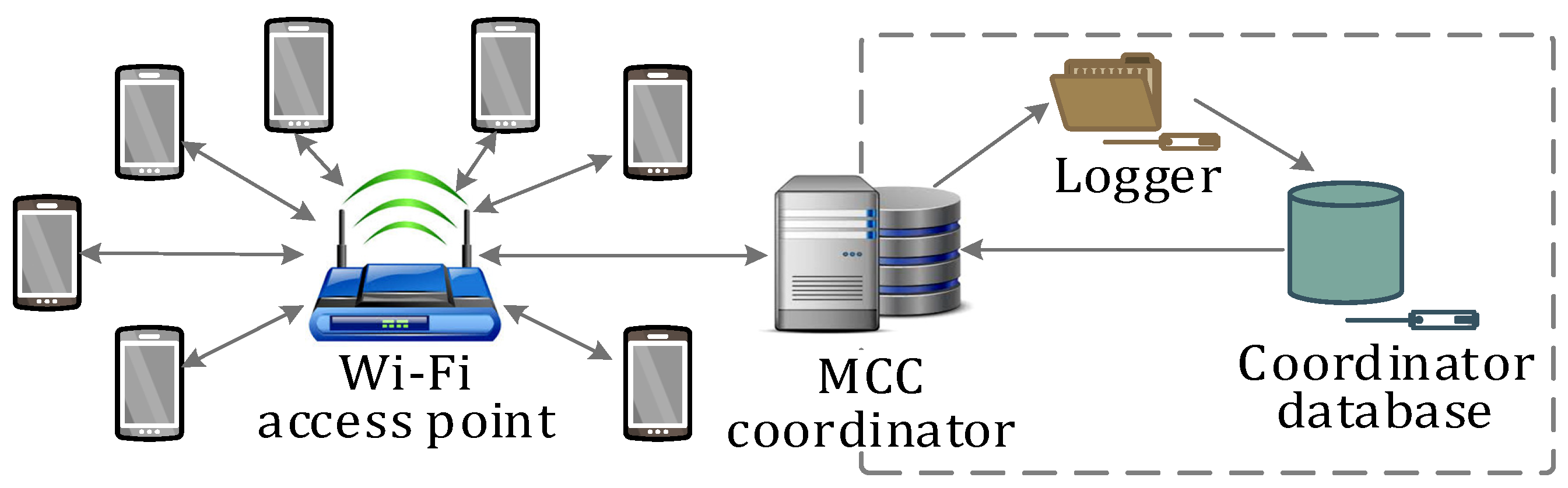
1.1. Mobile Crowd Computing
1.2. Resource Selection in Mobile Crowd Computing
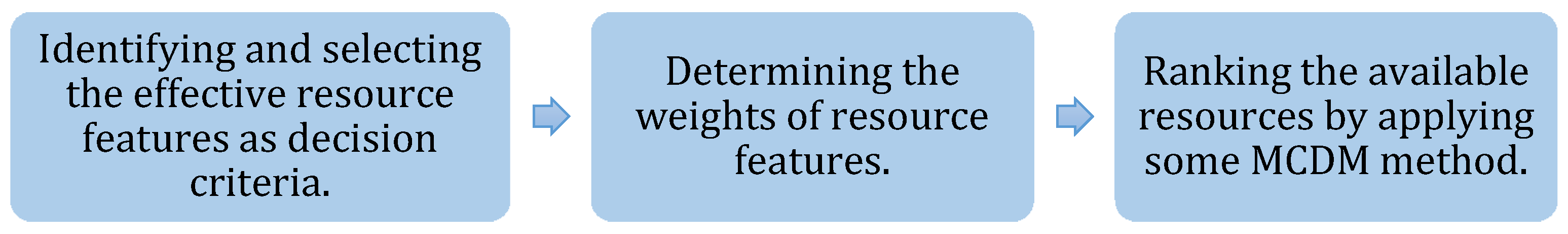
1.3. Resource Selection as an MCDM Problem
1.4. Paper Objective
1.5. Paper Contribution
- We use five distinct MCDM algorithms for the comparative analysis—EDAS, ARAS, MABAC, COPRAS, and MARCOS.
- The five algorithms that are used in this study are of distinctive nature in terms of their fundamental procedure. Moreover, the combination of the considered MCDM methods comprises some popularly used methods and some recently proposed methods. This diverse combination for a comparative study of MCDM methods is quite rare in the literature.
- To check the impact of the number of alternatives and criteria on the performance of the MCDM methods, we consider four data sets of different sizes. Each of the methods is implemented on all four datasets.
- We carry out an extensive comparative analysis of the results for all the considered scenarios under different variations of criteria and alternative sets. The comparative analysis is done on two aspects: (a) an exhaustive validation and robustness check and (b) the time complexity of each method.
- Along with the time complexity of each MCDM method, the actual runtime of each method on two different types of devices (laptop and smartphone) are compared and analyzed for each considered scenario.
- We found hardly any work in which computational and runtime-based comparison of different MCDM methods has been carried out apart from the validation and robustness check. To be specific, this paper is the first of its kind that compares the MCDM methods of different categories for resource selection in MCC or any other distributed mobile computing systems.
1.6. Paper Organization
2. Related Work
3. Research Background
3.1. MCDM Methods Considered for the Comparative Study
- (a)
- Separation from average solution (EDAS method).
- (b)
- The relative positioning of the alternatives with respect to the best one (ARAS method).
- (c)
- Utility-based classification and preferential ordering on the proportional scale (COPRAS method).
- (d)
- Approximation of the positions of the alternatives to the average solution area (MABAC method).
- (e)
- Compromise solution while trading of the effects of the criteria on the alternatives (MARKOS method).
3.1.1. EDAS Method
3.1.2. ARAS Method
3.1.3. MABAC Method
3.1.4. COPRAS Method
3.1.5. MARCOS Method
3.2. Entropy Method for Criteria Weight Calculation
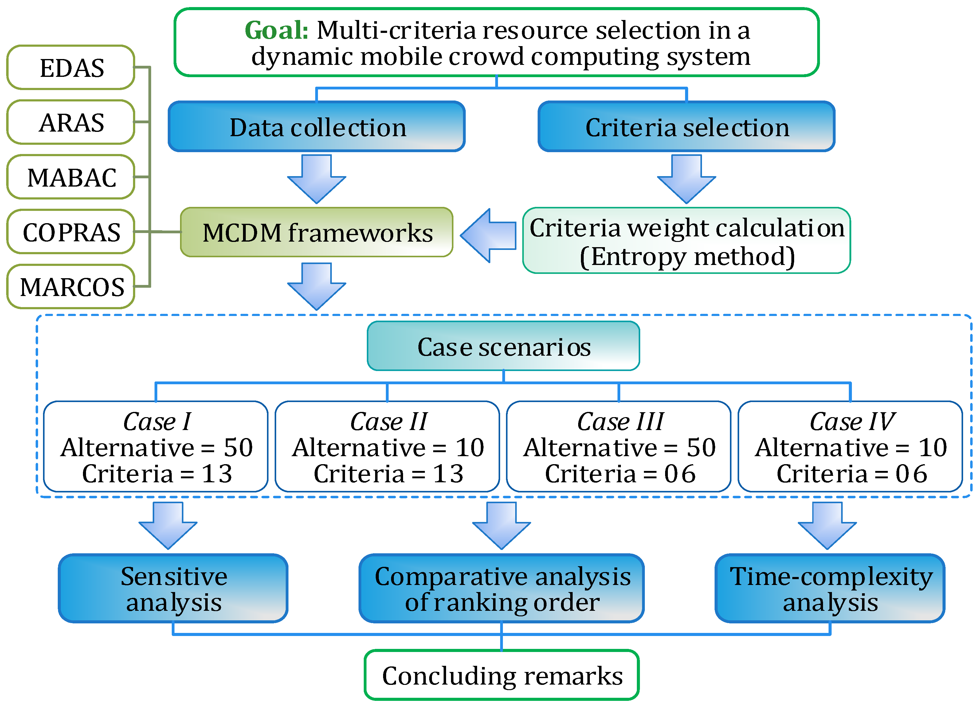
4. Research Methodology
4.1. Resource Selection Criteria
4.2. Data Collection
4.3. Experiment Cases
4.3.1. Case 1: Full List of Alternatives and Full Criteria Set
4.3.2. Case 2: Lesser Number of Alternatives and Full Criteria Set
4.3.3. Case 3: Total Number of Alternatives and a Smaller Number of Criteria
4.3.4. Case 4: Minimized Number of Alternatives and Criteria
5. Experiment, Results, and Comparative Analysis
5.1. Experiment
5.2. Results
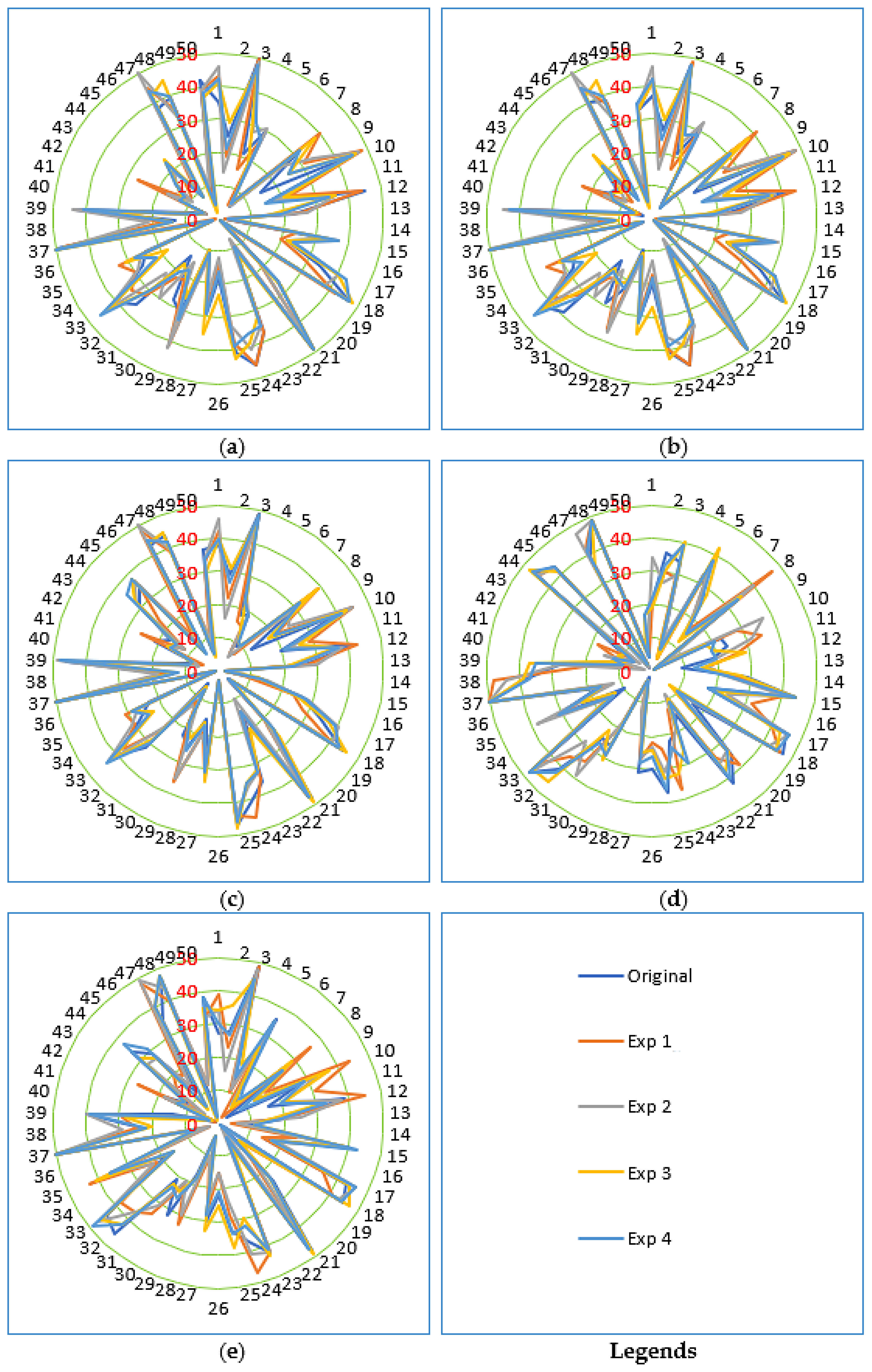
5.3. Sensitivity Analysis
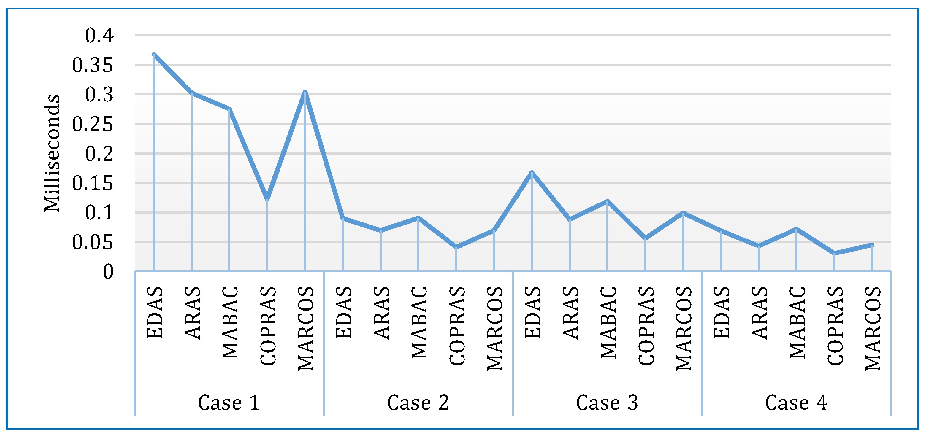
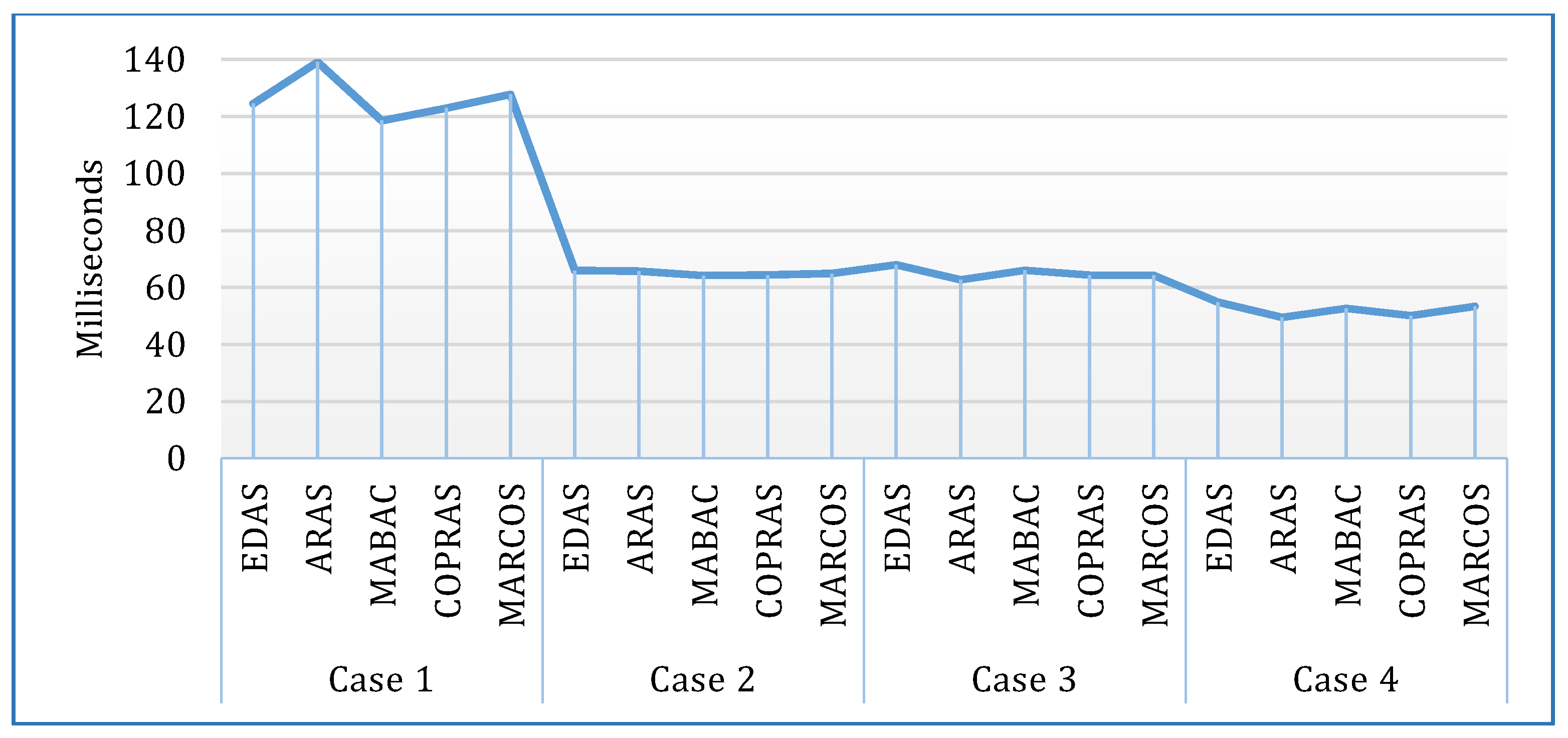
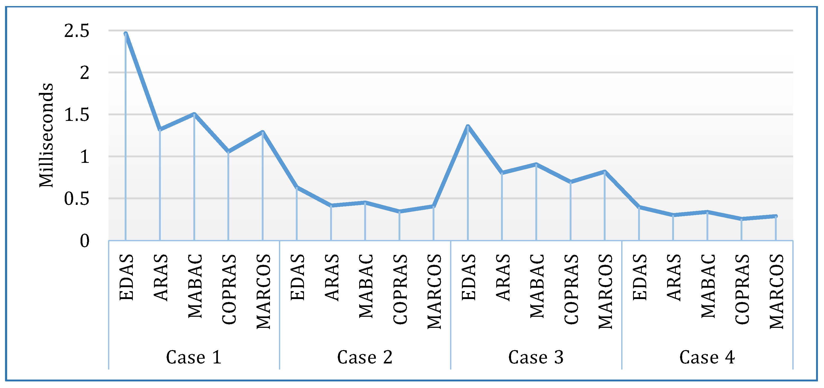
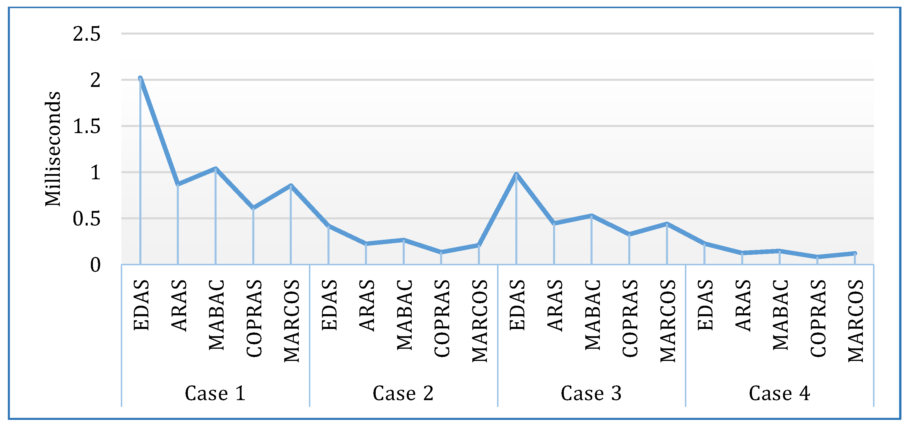
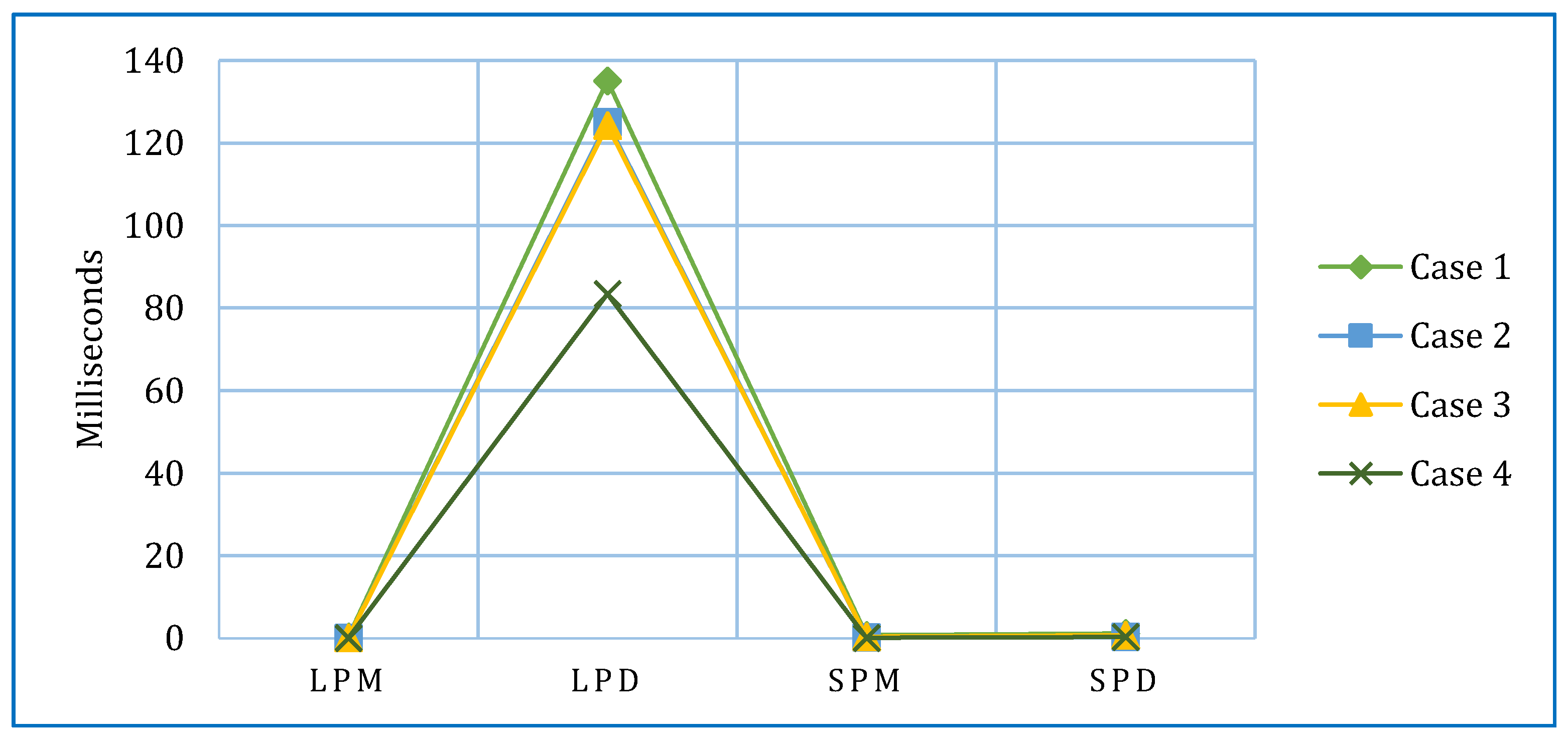
5.4. Time Complexity Analysis
6. Discussion
6.1. Findings and Observations
- Condition 1: Full set (Case 1: complete set of 13 criteria and 50 alternatives)
- Condition 2: Reduction in the number of alternatives keeping the criteria set unaltered (Case 2: reduced set of 10 alternatives and complete set of 13 criteria)
- Condition 3: Variation in the criteria set (Case 3: reduced set of 6 criteria) keeping the alternative set the same (i.e., 50)
- Condition 4: Variations in both alternative and criteria sets (Case 4: reduced set of 10 alternatives and 6 criteria).
6.2. Rationality and Practicability
6.2.1. Assertion
6.2.2. Application
6.2.3. Implications
7. Conclusions, Limitations, and Further Research Scope
7.1. Summary
7.2. Observation
7.3. Conclusive Statement
7.4. Limitations and Improvement Scopes
7.5. Open Research Prospects
Author Contributions
Funding
Institutional Review Board Statement
Informed Consent Statement
Data Availability Statement
Acknowledgments
Conflicts of Interest
References
- Falaki, H.; Mahajan, R.; Kandula, S.; Lymberopoulos, D.; Govindan, R.; Estrin, D. Diversity in smartphone usage. In Proceedings of the 8th International Conference on Mobile Systems, Applications, and Services (MobiSys 2010), San Francisco, CA, USA, 15–18 June 2010. [Google Scholar]
- Wagner, D.T.; Rice, A.; Beresford, A.R. Device Analyzer: Understanding smartphone usage. In Mobile and Ubiquitous Systems: Computing Networking and Services; Springer International Publishing: Berlin/Heidelberg, Germany, 2014; Volume 131, pp. 195–208. [Google Scholar]
- Wurmser, Y. US Time Spent with Mobile 2019. 30 May 2019. Available online: https://www.emarketer.com/content/us-time-spent-with-mobile-2019 (accessed on 9 April 2021).
- Loke, S.W.; Napier, K.; Alali, A.; Fernando, N.; Rahayu, W. Mobile Computations with Surrounding Devices: Proximity Sensing and MultiLayered Work Stealing. ACM Trans. Embed. Comput. Syst. 2015, 14, 1–25. [Google Scholar] [CrossRef]
- Mtibaa, K.; Harras, A.; Habak, K.; Ammar, M.; Zegura, E.W. Towards Mobile Opportunistic Computing. In Proceedings of the IEEE 8th International Conference on Cloud Computing, New York, NY, USA, 27 June–2 July 2015. [Google Scholar]
- Lavoie, E.; Hendren, L. Personal volunteer computing. In Proceedings of the 16th ACM International Conference on Computing Frontiers (CF ‘19), Alghero, Italy, 30 April–2 May 2019. [Google Scholar]
- Fernando, N.; Loke, S.W.; Rahayu, W. Mobile Crowd Computing with Work Stealing. In Proceedings of the 15th International Conference on Network-Based Information Systems, Melbourne, Australia, 26–28 September 2012. [Google Scholar]
- Pramanik, P.K.D.; Choudhury, P.; Saha, A. Economical Supercomputing thru Smartphone Crowd Computing: An Assessment of Opportunities, Benefits, Deterrents, and Applications from India’s Perspective. In Proceedings of the 4th International Conference on Advanced Computing and Communication Systems (ICACCS—2017), Coimbatore, India, 6–7 January 2017. [Google Scholar]
- Pramanik, P.K.D.; Pal, S.; Choudhury, P. Smartphone Crowd Computing: A Rational Approach for Sustainable Computing by Curbing the Environmental Externalities of the Growing Computing Demands. In Emerging Trends in Disruptive Technology Management; Das, R., Banerjee, M., De, S., Eds.; Chapman and Hall/CRC: Boca Raton, FL, USA, 2019. [Google Scholar]
- Pramanik, P.K.D.; Pal, S.; Choudhury, P. Green and Sustainable High-Performance Computing with Smartphone Crowd Computing: Benefits, Enablers, and Challenges. Scalable Comput. Pract. Exp. 2019, 20, 259–283. [Google Scholar] [CrossRef]
- Pramanik, P.K.D.; Choudhury, P. Mobility-aware service provisioning for delay tolerant applications in a mobile crowd computing environment. SN Appl. Sci. 2020, 2, 1–17. [Google Scholar] [CrossRef] [Green Version]
- O’Dea, S. Smartphone Users Worldwide 2016–2023. 31 March 2021. Available online: https://www.statista.com/statistics/330695/number-of-smartphone-users-worldwide/ (accessed on 9 April 2021).
- Loke, S.W. Crowd-Powered Mobile Computing and Smart Things; Springer Briefs in Computer Science; Springer: Cham, Switzerland, 2017. [Google Scholar]
- Pramanik, P.K.D.; Choudhury, P. IoT Data Processing: The Different Archetypes and their Security & Privacy Assessments. In Internet of Things (IoT) Security: Fundamentals Techniques and Applications; Shandilya, S.K., Chun, S.A., Shandilya, S., Weippl, E., Eds.; River Publishers: Gistrup, Denmark, 2018; pp. 37–54. [Google Scholar]
- Pramanik, P.K.D.; Pal, S.; Brahmachari, A.; Choudhury, P. Processing IoT Data: From Cloud to Fog. It’s Time to be Down-to-Earth. In Applications of Security Mobile Analytic and Cloud (SMAC) Technologies for Effective Information Processing and Management; Karthikeyan, P., Thangavel, M., Eds.; IGI Global: Hershey, PA, USA, 2018; pp. 124–148. [Google Scholar]
- Miluzzo, E.; Cáceres, R.; Chen, Y.-F. Vision: mClouds—Computing on Clouds of Mobile Devices. In Proceedings of the 3rd ACM Workshop on Mobile Cloud Computing and Services (MCS’12), Low Wood Bay, Lake District, UK, 25 June 2012. [Google Scholar]
- Marinelli, E.E. Hyrax: Cloud Computing on Mobile Devices Using. Master’s Thesis, Carnegie Mellon University, Pittsburgh, PA, USA, 2009. [Google Scholar]
- Shila, D.M.; Shen, W.; Cheng, Y.; Tian, X.; Shen, X.S. AMCloud: Toward a Secure Autonomic Mobile Ad Hoc Cloud Computing System. IEEE Wirel. Commun. 2017, 24, 74–81. [Google Scholar] [CrossRef]
- Hirsch, M.; Mateos, C.; Zunino, A. Augmenting computing capabilities at the edge by jointly exploiting mobile devices: A survey. Future Gener. Comput. Syst. 2018, 88, 644–662. [Google Scholar] [CrossRef]
- Fernando, N.; Loke, S.W.; Rahayu, W. Computing with Nearby Mobile Devices: A Work Sharing Algorithm for Mobile Edge-Clouds. IEEE Trans. Cloud Comput. 2019, 7, 329–343. [Google Scholar] [CrossRef]
- Habak, K.; Ammar, M.; Harras, K.A.; Zegura, E. Femto Clouds: Leveraging Mobile Devices to Provide Cloud Service at the Edge. In Proceedings of the IEEE 8th International Conference on Cloud Computing, New York, NY, USA, 27 June–2 July 2015. [Google Scholar]
- Zhou, A.; Wang, S.; Li, J.; Sun, Q.; Yang, F. Optimal mobile device selection for mobile cloud service providing. J. Supercomput. 2016, 72, 3222–3235. [Google Scholar] [CrossRef]
- Kandappu, T.; Misra, A.; Cheng, S.-F.; Jaiman, N.; Tandriansiyah, R.; Chen, C.; Lau, H.C.; Chander, D.; Dasgupta, K. Campus-Scale Mobile Crowd-Tasking: Deployment & Behavioral Insights. In Proceedings of the 19th ACM Conference on Computer-Supported Cooperative Work & Social Computing (CSCW 16), San Francisco, CA, USA, 26 February–2 March 2016. [Google Scholar]
- McKnight, L.W.; Howison, J.; Bradner, S. Guest Editors’ Introduction: Wireless Grids—Distributed Resource Sharing by Mobile, Nomadic, and Fixed Devices. IEEE Internet Comput. 2004, 8, 24–31. [Google Scholar] [CrossRef]
- Mohamed, M.M.; Srinivas, A.V.; Janakiram, D. Moset: An anonymous remote mobile cluster computing paradigm. J. Parallel Distrib. Comput. 2005, 65, 1212–1222. [Google Scholar] [CrossRef]
- Kumar, M.P.; Bhat, R.R.; Alavandar, S.R.; Ananthanarayana, V.S. Distributed Public Computing and Storage using Mobile Devices. In Proceedings of the IEEE Distributed Computing, VLSI, Electrical Circuits and Robotics (DISCOVER), Mangalore, India, 13–14 August 2018. [Google Scholar]
- Curiel, M.; Calle, D.F.; Santamaría, A.S.; Suarez, D.F.; Flórez, L. Parallel Processing of Images in Mobile Devices using BOINC. Open Eng. 2018, 8, 87–101. [Google Scholar] [CrossRef]
- Yaqoob, I.; Ahmed, E.; Gani, A.; Mokhtar, S.; Imran, M. Heterogeneity-aware task allocation in mobile ad hoc cloud. IEEE Access 2017, 5, 1779–1795. [Google Scholar] [CrossRef]
- Žižović, M.; Pamučar, D.; Albijanić, M.; Chatterjee, P.; Pribićević, I. Eliminating Rank Reversal Problem Using a New Multi-Attribute Model—The RAFSI Method. Mathematics 2020, 8, 1015. [Google Scholar] [CrossRef]
- Hwang, C.L.; Yoon, K. Multiple Attribute Decision Making: Methods and Applications; Springer: New York, NY, USA, 1981. [Google Scholar]
- Hwang, C.-L.; Lai, Y.-J.; Liu, T.-Y. A new approach for multiple objective decision making. Comput. Oper. Res. 1993, 20, 889–899. [Google Scholar] [CrossRef]
- Ghorabaee, M.K.; Zavadskas, E.K.; Olfat, L.; Turskis, Z. Multi-criteria inventory classification using a new method of evaluation based on distance from average solution (EDAS). Informatica 2015, 26, 435–451. [Google Scholar] [CrossRef]
- Pamučar, D.; Ćirović, G. The selection of transport and handling resources in logistics centers using Multi-Attributive Border Approximation area Comparison (MABAC). Expert Syst. Appl. 2015, 42, 3016–3028. [Google Scholar] [CrossRef]
- Alinezhad, A.; Khalili, J. MABAC Method. In New Methods and Applications in Multiple Attribute Decision Making (MADM); International Series in Operations Research & Management Science; Springer: Berlin/Heidelberg, Germany, 2019; Volume 277, pp. 193–198. [Google Scholar]
- Zavadskas, E.K.; Turskis, Z. A new additive ratio assessment (ARAS) method in multicriteria decision-making. Technol. Econ. Dev. Econ. 2010, 16, 159–172. [Google Scholar] [CrossRef]
- Alinezhad, A.; Khalili, J. ARAS Method. In New Methods and Applications in Multiple Attribute Decision Making (MADM); International Series in Operations Research & Management Science; Springer: Berlin/Heidelberg, Germany, 2019; Volume 277, pp. 67–71. [Google Scholar]
- MacCrimmon, R. Decisionmaking among Multiple-Attribute Alternatives: A Survey and Consolidated Approach; Research Memorandum: Santa Monica, CA, USA, 1968. [Google Scholar]
- Zavadskas, E.K.; Kaklauskas, A.; Sarka, V. The new method of multi-criteria complex proportional assessment of projects. Technol. Econ. Dev. Econ. 1994, 1, 131–139. [Google Scholar]
- Alinezhad, A.; Khalili, J. COPRAS Method. In New Methods and Applications in Multiple Attribute Decision Making (MADM); International Series in Operations Research & Management Science; Springer: Berlin/Heidelberg, Germany, 2019; Volume 277, pp. 87–91. [Google Scholar]
- Duckstein, L.; Opricovic, S. Multiobjective optimization in river basin development. Water Resour. Res. 1980, 16, 14–20. [Google Scholar] [CrossRef]
- Opricovic, S.; Tzeng, G.H. Compromise solution by MCDM methods: A comparative analysis of VIKOR and TOPSIS. Eur. J. Oper. Res. 2004, 156, 445–455. [Google Scholar] [CrossRef]
- Yazdani, P.; Zarate, E.K.; Zavadskas, E.; Turskis, T. A Combined Compromise Solution (CoCoSo) method for multi-criteria decision-making problems. Manag. Decis. 2019, 57, 2501–2519. [Google Scholar] [CrossRef]
- Stević, Ž.; Pamučar, D.; Puška, A.; Chatterjee, P. Sustainable supplier selection in healthcare industries using a new MCDM method: Measurement of alternatives and ranking according to COmpromise solution (MARCOS). Comput. Ind. Eng. 2020, 140, 106231. [Google Scholar] [CrossRef]
- Mardani, A.; Jusoh, K.M.; Nor, Z.; Khalifah, N.; Zakwan, N.; Valipour, A. Multiple criteria decision-making techniques and their applications—A review of the literature from 2000 to 2014. Econ. Res.-Ekon. Istraživanja 2015, 28, 516–571. [Google Scholar] [CrossRef]
- Zavadskas, E.K.; Turskis, Z.; Kildienė, S. State of art surveys of overviews on MCDM/MADM methods. Technol. Econ. Dev. Econ. 2014, 20, 165–179. [Google Scholar] [CrossRef] [Green Version]
- Zavadskas, E.K.; Antucheviciene, J.; Adeli, H.; Turskis, Z.; Adeli, H. Hybrid multiple criteria decision making methods: A review of applications in engineering. Sci. Iran. 2016, 23, 1–20. [Google Scholar]
- Hosseinzadeh, H.K.; Hama, M.Y.; Ghafour, M.; Masdari, O.H.; Ahmed, H.; Khezri, H. Service Selection Using Multi-criteria Decision Making: A Comprehensive Overview. J. Netw. Syst. Manag. 2020, 28, 1639–1693. [Google Scholar] [CrossRef]
- Bagga, P.; Joshi, A.; Hans, R. QoS based Web Service Selection and Multi-Criteria Decision Making Methods. Int. J. Interact. Multimed. Artif. Intell. 2019, 5, 113–121. [Google Scholar] [CrossRef] [Green Version]
- Grgurević, I.; Kordić, G. Multi-criteria Decision-making in Cloud Service Selection and Adoption. In Proceedings of the 5th International Virtual Research Conference in Technical Disciplines, 2017. Available online: https://www.bib.irb.hr/905215?rad=905215 (accessed on 9 April 2021).
- Hamzeh, A.; Ahmad, K.; Noreen, A.; Deemah, A. Cloud service evaluation method-based Multi-Criteria Decision-Making: A systematic literature review. J. Syst. Softw. 2018, 139, 161–188. [Google Scholar]
- Büyüközkan, G.; Göçer, F.; Feyzioğlu, O. Cloud computing technology selection based on interval-valued intuitionistic fuzzy MCDM methods. Soft Comput. 2018, 22, 5091–5114. [Google Scholar] [CrossRef]
- Youssef, E. An Integrated MCDM Approach for Cloud Service Selection Based on TOPSIS and BWM. IEEE Access 2020, 8, 71851–71865. [Google Scholar] [CrossRef]
- Singla, C.; Mahajan, N.; Kaushal, S.; Verma, A.; Sangaiah, K. Modelling and Analysis of Multi-objective Service Selection Scheme in IoT-Cloud Environment. In Cognitive Computing for Big Data Systems Over IoT. Lecture Notes on Data Engineering and Communications Technologies; Sangaiah, A., Thangavelu, A., Sundaram, V.M., Eds.; Springer: Cham, Switzerland, 2018; Volume 14, pp. 63–77. [Google Scholar]
- Wu, H. Multi-Objective Decision-Making for Mobile Cloud Offloading: A Survey. IEEE Access 2018, 6, 3962–3976. [Google Scholar] [CrossRef]
- Bangui, H.; Ge, M.; Buhnova, B.; Rakrak, S.; Raghay, S.; Pitner, T. Multi-Criteria Decision Analysis Methods in the Mobile Cloud Offloading Paradigm. J. Sens. Actuator Netw. 2017, 6, 25. [Google Scholar] [CrossRef] [Green Version]
- Ravi, S.; Peddoju, K. Handoff Strategy for Improving Energy Efficiency and Cloud Service Availability for Mobile Devices. Wirel. Pers. Commun. 2015, 81, 101–132. [Google Scholar] [CrossRef]
- Mishra, K.; Ray, N.K.; Swain, A.R.; Mund, G.B.; Mishra, B.S.P. An adaptive model for resource selection and allocation in fog computing environment. Comput. Electr. Eng. 2019, 77, 217–229. [Google Scholar] [CrossRef]
- Gad-ElRab, A.; Alsharkawy, A.S. Multiple criteria-based efficient schemes for participants selection in mobile crowd sensing. Int. J. Commun. Netw. Distrib. Syst. 2018, 21, 384–417. [Google Scholar] [CrossRef]
- Nik, W.N.S.W.; Zhou, B.B.; Abawajy, J.H.; Zomaya, A.Y. Cost and Performance-Based Resource Selection Scheme for Asynchronous Replicated System in Utility-Based Computing Environment. Int. J. Adv. Sci. Eng. Inf. Technol. 2017, 7, 723–735. [Google Scholar] [CrossRef] [Green Version]
- Mohammadi, S.; Homayoun, S.; Zadeh, E.T. Grid Computing: Strategic Decision Making in Resource Selection. Int. J. Comput. Sci. Eng. Appl. 2012, 2, 1–12. [Google Scholar] [CrossRef]
- Abdullah, M.; Ali, H.A.; Haikal, A.Y. A reliable, TOPSIS-based multi-criteria, and hierarchical load balancing method for computational grid. Clust. Comput. 2019, 22, 1085–1106. [Google Scholar] [CrossRef]
- Kaur, M.; Kadam, S.S. Discovery of resources using MADM approaches for parallel and distributed computing. Eng. Sci. Technol. Int. J. 2017, 20, 1013–1024. [Google Scholar] [CrossRef]
- Yildiz, A.; Ergül, E.U. A two-phased multi-criteria decision-making approach for selecting the best smartphone. S. Afr. J. Ind. Eng. 2015, 26, 1208. [Google Scholar] [CrossRef] [Green Version]
- Büyüközkan, G.; Güleryüz, S. Multi Criteria Group Decision Making Approach for Smart Phone Selection Using Intuitionistic Fuzzy TOPSIS. Int. J. Comput. Intell. Syst. 2016, 9, 709–725. [Google Scholar] [CrossRef] [Green Version]
- Goswami, S.S.; Behera, D.K. Evaluation of the best smartphone model in the market by integrating fuzzy-AHP and PROMETHEE decision-making approach. Decis. Off. J. Indian Inst. Manag. Calcutta 2021, 48, 71–96. [Google Scholar]
- Kumar, S.; Singh, S.K.; Kumar, T.A.; Agrawal, S. Research Methodology: Prioritization of New Smartphones Using TOPSIS and MOORA. In Proceedings of the International Conference of Advance Research & Innovation (ICARI), Meerut, India, 30 January 2020. [Google Scholar]
- Aggarwal, A.; Choudhary, C.; Mehrotra, D. Evaluation of smartphones in Indian market using EDAS. Procedia Comput. Sci. 2019, 132, 236–243. [Google Scholar] [CrossRef]
- Irvanizam, I.; Marzuki, M.; Patria, I.; Abubakar, R. An Application for Smartphone Preference Using TODIM Decision Making Method. In Proceedings of the International Conference on Electrical Engineering and Informatics (ICELTICs), Banda Aceh, Indonesia, 19–20 September 2018. [Google Scholar]
- Abdulhadi, Q. Selection a New Mobile Phone by Utilize the Voting Method, AHP and Enhance TOPSIS. Int. J. Acad. Res. Bus. Soc. Sci. 2020, 10, 717–732. [Google Scholar]
- Triantaphyllou, E. Multi-Criteria Decision Making Methods: A Comparative Study; Springer: Boston, MA, USA, 2000. [Google Scholar]
- Velasquez, M.; Hester, P.T. An Analysis of Multi-Criteria Decision Making Methods. Int. J. Oper. Res. 2013, 10, 56–66. [Google Scholar]
- Danesh, D.; Ryan, M.J.; Abbasi, A. Multi-criteria decision-making methods for project portfolio management: A literature review. Int. J. Manag. Decis. Mak. 2017, 17, 75. [Google Scholar] [CrossRef]
- Marqués, I.; García, V.; Sánchez, J.S. Ranking-based MCDM models in financial management applications: Analysis and emerging challenges. Prog. Artif. Intell. 2020, 9, 171–193. [Google Scholar] [CrossRef]
- Purwita, A.; Subriadi, A. Literature Review—Using Multi-Criteria Decision-Making Methods in Information Technology (IT) Investment. In Proceedings of the 1st International Conference on Business Law and Pedagogy (ICBLP 2019), Sidoarjo, Indonesia, 13–15 February 2019. [Google Scholar]
- Özkan, B.; Özceylan, E.; Sarıçiçek, İ. GIS-based MCDM modeling for landfill site suitability analysis: A comprehensive review of the literature. Environ. Sci. Pollut. Res. 2019, 26, 30711–30730. [Google Scholar] [CrossRef] [PubMed]
- Alkaradaghi, K.; Ali, S.S.; Al-Ansari, N.; Laue, J.; Chabuk, A. Landfill Site Selection Using MCDM Methods and GIS in the Sulaimaniyah Governorate, Iraq. Sustainability 2019, 11, 4530. [Google Scholar] [CrossRef] [Green Version]
- Arıkan, E.; Vayvay, Z.T.-K.Ö. Solid waste disposal methodology selection using multi-criteria decision making methods and an application in Turkey. J. Clean. Prod. 2017, 142, 403–412. [Google Scholar] [CrossRef]
- Coban, A.; Ertis, I.F.; Cavdaroglu, N.A. Municipal solid waste management via multi-criteria decision making methods: A case study in Istanbul, Turkey. J. Clean. Prod. 2018, 180, 159–167. [Google Scholar] [CrossRef]
- Stojčić, M.; Zavadskas, E.K.; Pamučar, D.; Stević, Ž.; Mardani, A. Application of MCDM Methods in Sustainability Engineering: A Literature Review 2008–2018. Symmetry 2019, 11, 350. [Google Scholar] [CrossRef] [Green Version]
- Okpako, E.; Oghenenyerovwho, S. Application of MCDM method in material selection for optimal design: A review. Results Mater. 2020, 7, 100115. [Google Scholar]
- Singarave, B.; Shankar, D.P.; Prasanna, L. Application of MCDM Method for the Selection of Optimum Process Parameters in Turning Process. Mater. Today Proc. 2018, 5, 13464–13471. [Google Scholar] [CrossRef]
- Shafiee, M. Maintenance strategy selection problem: An MCDM overview. J. Qual. Maint. Eng. 2015, 21, 378–402. [Google Scholar] [CrossRef]
- Brzozowski, M.; Birfer, I. Applications of MCDM Methods in the ERP System Selection Process in Enterprises. Handel Wewnętrzny 2017, 3, 40–52. [Google Scholar]
- Utama, W.P.; Chan, A.P.; Gao, R.; Zahoor, H. Making international expansion decision for construction enterprises with multiple criteria: A literature review approach. Int. J. Constr. Manag. 2018, 18, 221–231. [Google Scholar] [CrossRef]
- Chowdhury, P.; Paul, S.K. Applications of MCDM methods in research on corporate sustainability: A systematic literature review. Manag. Environ. Qual. 2020, 31, 385–405. [Google Scholar] [CrossRef]
- Asgari, N.; Darestani, S.A. Application of multi-criteria decision making methods for balanced scorecard: A literature review investigation. Int. J. Serv. Oper. Manag. 2017, 27, 272. [Google Scholar]
- Zavadskas, K.; Antucheviciene, J.; Chatterjee, P. Multiple-Criteria Decision-Making (MCDM) Techniques for Business Processes Information Management. Information 2019, 10, 4. [Google Scholar] [CrossRef] [Green Version]
- Almeida, T.D.; Alencar, M.H.; Garcez, T.V.; Ferreira, R.J.P. A systematic literature review of multicriteria and multi-objective models applied in risk management. IMA J. Manag. Math. 2017, 28, 153–184. [Google Scholar] [CrossRef]
- Mukul, E.; Büyüközkan, G.; Güler, M. Evaluation of Digital Marketing Technologies with Mcdm Methods. In Proceedings of the 6th International Conference on New Ideas in Management Economics and Accounting, France, Paris, 19–21 April 2019. [Google Scholar]
- Jusoh, A.; Mardani, A.; Omar, R.; Štreimikienė, D.; Khalifah, Z.; Sharifara, A. Application of MCDM approach to evaluate the critical success factors of total quality management in the hospitality industry. J. Bus. Econ. Manag. 2018, 19, 399–416. [Google Scholar] [CrossRef] [Green Version]
- Salomon, V. (Ed.) Multi-Criteria Methods and Techniques Applied to Supply Chain Management; IntechOpen: London, UK, 2018. [Google Scholar]
- Schramm, V.B.; Cabral, L.P.B.; Schramm, F. Approaches for supporting sustainable supplier selection—A literature review. J. Clean. Prod. 2020, 273, 123089. [Google Scholar] [CrossRef]
- Yildiz, A.; Yayla, A.Y. Multi-criteria decision-making methods for supplier selection: A literature review. S. Afr. J. Ind. Eng. 2015, 26, 158–177. [Google Scholar] [CrossRef] [Green Version]
- Govindan, K.; Rajendran, S.; Sarkis, J.; Murugesan, P. Multi criteria decision making approaches for green supplier evaluation and selection: A literature review. J. Clean. Prod. 2015, 98, 66–83. [Google Scholar] [CrossRef]
- Kaya, İ.; Çolak, M.; Terzi, F. Use of MCDM techniques for energy policy and decision-making problems: A review. Int. J. Energy Res. 2018, 42, 2344–2372. [Google Scholar] [CrossRef]
- Siksnelyte-Butkiene, I.; Zavadskas, E.K.; Streimikiene, D. Multi-Criteria Decision-Making (MCDM) for the Assessment of Renewable Energy Technologies in a Household: A Review. Energies 2020, 13, 1164. [Google Scholar] [CrossRef] [Green Version]
- Kumar, A.; Sah, B.; Singh, A.R.; Deng, Y.; He, X.; Kumar, P.; Bansal, R.C. A review of multi criteria decision making (MCDM) towards sustainable renewable energy development. Renew. Sustain. Energy Rev. 2017, 69, 596–609. [Google Scholar] [CrossRef]
- Shao, M.; Han, Z.; Sun, J.; Xiao, C.; Zhang, S.; Zhao, Y. A review of multi-criteria decision making applications for renewable energy site selection. Renew. Energy 2020, 157, 377–403. [Google Scholar] [CrossRef]
- Antucheviciene, J.; Kala, Z.; Marzouk, M.; Vaidogas, E.R. Decision Making Methods and Applications in Civil Engineering. Math. Probl. Eng. 2015, 2015, 160569. [Google Scholar] [CrossRef]
- Zavadskas, K.; Antuchevičienė, J.; Kapliński, O. Multi-criteria decision making in civil engineering. Part II—Applications. Eng. Struct. Technol. 2015, 7, 151–167. [Google Scholar] [CrossRef]
- Penadés-Plà, V.; García-Segura, T.; Martí, J.V.; Yepes, V. A Review of Multi-Criteria Decision-Making Methods Applied to the Sustainable Bridge Design. Sustainability 2016, 8, 1295. [Google Scholar] [CrossRef] [Green Version]
- Tan, T.; Mills, G.; Papadonikolaki, E.; Liu, Z. Combining multi-criteria decision making (MCDM) methods with building information modelling (BIM): A review. Autom. Constr. 2021, 121, 103451. [Google Scholar] [CrossRef]
- Pavlovskis, M.; Antucheviciene, J.; Migilinskas, D. Application of MCDM and BIM for Evaluation of Asset Redevelopment Solutions. Stud. Inform. Control 2016, 25, 293–302. [Google Scholar] [CrossRef] [Green Version]
- Si, J.; Marjanovic-Halburd, L.; Nasiri, F.; Bell, S. Assessment of building-integrated green technologies: A review and case study on applications of Multi-Criteria Decision Making (MCDM) method. Sustain. Cities Soc. 2016, 27, 106–115. [Google Scholar] [CrossRef]
- Gibari, S.E.; Gómez, T.; Ruiz, F. Building composite indicators using multicriteria methods: A review. J. Bus. Econ. 2019, 89, 1–24. [Google Scholar] [CrossRef]
- Morkūnaitė, Ž.; Kalibatas, D.; Kalibatienė, D. A bibliometric data analysis of multi-criteria decision making methods in heritage buildings. J. Civ. Eng. Manag. 2019, 25, 76–99. [Google Scholar] [CrossRef]
- Hoang, T.T.; Dupont, L.; Camargo, M. Application of Decision-Making Methods in Smart City Projects: A Systematic Literature Review. Smart Cities 2019, 2, 433–452. [Google Scholar] [CrossRef] [Green Version]
- Gebre, S.L.; Cattrysse, D.; Orshoven, J.V. Multi-Criteria Decision-Making Methods to Address Water Allocation Problems: A Systematic Review. Water 2021, 13, 125. [Google Scholar] [CrossRef]
- Hassan, S.A.H.S.; Tan, S.C.; Yusof, K.M. MCDM for Engineering Education: Literature Review and Research Issues. In Engineering Education for a Smart Society (GEDC 2016 WEEF 2016). Advances in Intelligent Systems and Computing; Auer, M., Kim, K.S., Eds.; Springer: Cham, Switzerland, 2018; Volume 627, pp. 204–214. [Google Scholar]
- Zare, M.; Pahl, C.; Rahnama, H.; Nilashi, M.; Mardani, A.; Ibrahim, O.; Ahmadi, H. Multi-criteria decision making approach in E-learning: A systematic review and classification. Appl. Soft Comput. 2016, 45, 108–128. [Google Scholar] [CrossRef]
- Pal, S.; Pramanik, P.K.D.; Alsulami, M.; Nayyar, A.; Zarour, M.; Choudhury, P. Using DEMATEL for Contextual Learner Modelling in Personalised and Ubiquitous Learning. Comput. Mater. Contin. 2021, 69. [Google Scholar] [CrossRef]
- Khan, Z.; Ansari, T.S.A.; Siddiquee, A.N.; Khan, Z.A. Selection of E-learning websites using a novel Proximity Indexed Value (PIV) MCDM method. J. Comput. Educ. 2019, 6, 241–256. [Google Scholar] [CrossRef]
- Pekkaya, M. Career Preference of University Students: An Application of MCDM Methods. Procedia Econ. Financ. 2015, 23, 249–255. [Google Scholar] [CrossRef] [Green Version]
- Rajabi, F.; Molaeifar, H.; Jahangiri, M.; Taheri, S.; Banaee, S.; Farhadi, P. Occupational stressors among firefighters: Application of multi-criteria decision making (MCDM)Techniques. Heliyon 2020, 6, e03820. [Google Scholar] [CrossRef]
- Afshari, R.; Yusuff, R.M.; Hong, T.S.; Ismail, Y.B. A review of the applications of multi criteria decision making for personnel selection problem. Afr. J. Bus. Manag. 2011, 5, 28. [Google Scholar]
- Alp, S.; Özkan, T.K. Job Choice with Multi-Criteria Decision Making Approach in a Fuzzy Environment. Int. Rev. Manag. Mark. 2015, 5, 165–172. [Google Scholar]
- Pérez, C.; Carrillo, M.H.; Montoya-Torres, J.R. Multi-criteria approaches for urban passenger transport systems: A literature review. Ann. Oper. Res. 2015, 226, 69–87. [Google Scholar] [CrossRef]
- Kiciński, M.; Solecka, K. Application of MCDA/MCDM methods for an integrated urban public transportation system—Case study, city of Cracow. Arch. Transp. 2018, 46, 71–84. [Google Scholar] [CrossRef]
- Nassereddine, M.; Eskandari, H. An integrated MCDM approach to evaluate public transportation systems in Tehran. Transp. Res. Part A Policy Pract. 2017, 106, 427–439. [Google Scholar] [CrossRef] [Green Version]
- Yannis, G.; Kopsacheili, A.; Dragomanovits, A.; Petraki, V. State-of-the-art review on multi-criteria decision-making in the transport sector. J. Traffic Transp. Eng. 2020, 7, 413–431. [Google Scholar]
- Karacan, I.; Tozan, H.; Karatas, M. Multi Criteria Decision Methods in Health Technology Assessment: A Brief Literature Review. Eurasian J. Health Technol. Assess. 2016, 1, 12–19. [Google Scholar]
- Gul, M. A review of occupational health and safety risk assessment approaches based on multi-criteria decision-making methods and their fuzzy versions. Hum. Ecol. Risk Assess. Int. J. 2018, 24, 1723–1760. [Google Scholar] [CrossRef]
- Mutlu, M.; Tuzkaya, G.; Sennaroglu, B. Multi-criteria decision making techniques for healthcare service quality evaluation: A literature review. Sigma J. Eng. Nat. Sci. 2017, 35, 501–512. [Google Scholar]
- Zanakis, S.H.; Solomon, A.; Wisharta, N.; Dublish, S. Multi-attribute decision making: A simulation comparison of select methods. Eur. J. Oper. Res. 1998, 107, 507–529. [Google Scholar] [CrossRef]
- Annette, A.B.R.; Chandran, S.P. Comparison of multi criteria decision making algorithms for ranking cloud renderfarm services. Indian J. Sci. Technol. 2016, 9, 31. [Google Scholar]
- Piegat, A.; Sałabun, W. Comparative Analysis of MCDM Methods for Assessing the Severity of Chronic Liver Disease. In Proceedings of the Artificial Intelligence and Soft Computing (ICAISC 2015). Lecture Notes in Computer Science, Zakopane, Poland, 14–18 June 2015; Rutkowski, L., Korytkowski, M., Scherer, R., Tadeusiewicz, R., Zadeh, L., Zurada, J., Eds.; Springer: Cham, Switzerland, 2015; Volume 9119, pp. 228–238. [Google Scholar]
- Mathew, M.; Sahu, S. Comparison of new multi-criteria decision making methods for material handling equipment selection. Manag. Sci. Lett. 2018, 8, 139–150. [Google Scholar] [CrossRef]
- Ghosh, I.; Biswas, S. A comparative analysis of multi-criteria decision models for ERP package selection for improving supply chain performance. Asia-Pac. J. Manag. Res. Innov. 2016, 12, 250–270. [Google Scholar] [CrossRef]
- Nesticò, A.; Somma, P. Comparative Analysis of Multi-Criteria Methods forthe Enhancement of Historical Buildings. Sustainability 2019, 11, 4526. [Google Scholar] [CrossRef] [Green Version]
- Moradian, M.; Modanloo, V.; Aghaiee, S. Comparative analysis of multi criteria decision making techniques for material selection of brake booster valve body. J. Traffic Transp. Eng. 2019, 6, 526–534. [Google Scholar] [CrossRef]
- Ghaleb, M.; Kaid, H.; Alsamhan, A.; Mian, S.H.; Hidri, L. Assessment and Comparison of Various MCDM Approaches in the Selection of Manufacturing Process. Adv. Mater. Sci. Eng. 2020, 2020, 4039253. [Google Scholar] [CrossRef]
- Ceballos, M.T.; Lamata, D.; Pelta, A. A comparative analysis of multi-criteria decision-making methods. Prog. Artif. Intell. 2016, 5, 115–322. [Google Scholar] [CrossRef]
- Mulliner, E.; Malys, N.; Maliene, V. Comparative analysis of MCDM methods for the assessment of sustainable housing affordability. Omega 2016, 59, 146–156. [Google Scholar] [CrossRef]
- Vuković, M.; Pivac, S.; Babić, Z. Comparative analysis of stock selection using a hybrid MCDM approach and modern portfolio theory. Croat. Rev. Econ. Bus. Soc. Stat. 2020, 6, 58–68. [Google Scholar] [CrossRef]
- Sałabun, W.; Piegat, A. Comparative analysis of MCDM methods for the assessment of mortality in patients with acute coronary syndrome. Artif. Intell. Rev. 2017, 48, 557–571. [Google Scholar] [CrossRef]
- Valipour, A.; Sarvari, H.; Tamošaitiene, J. Risk Assessment in PPP Projects by Applying Different MCDM Methods and Comparative Results Analysis. Adm. Sci. 2018, 8, 80. [Google Scholar] [CrossRef] [Green Version]
- Lee, H.-C.; Chang, C.-T. Comparative analysis of MCDM methods for ranking renewable energy sources in Taiwan. Renew. Sustain. Energy Rev. 2018, 92, 883–896. [Google Scholar] [CrossRef]
- Karande, P.; Zavadskas, E.K.; Chakraborty, S. A study on the ranking performance of some MCDM methods for industrial robot selection problems. Int. J. Ind. Eng. Comput. 2016, 7, 399–422. [Google Scholar] [CrossRef]
- Harirchian, E.; Jadhav, K.; Mohammad, K.; Hosseini, S.E.A.; Lahmer, T. A Comparative Study of MCDM Methods Integrated with Rapid Visual Seismic Vulnerability Assessment of Existing RC Structures. Appl. Sci. 2020, 10, 6411. [Google Scholar] [CrossRef]
- Sidhu, J.; Singh, S. Design and Comparative Analysis of MCDM-based Multi-dimensional Trust Evaluation Schemes for Determining Trustworthiness of Cloud Service Providers. J. Grid Comput. 2017, 15, 197–218. [Google Scholar] [CrossRef]
- Alrababah, S.A.A.; Gan, K.H.; Tan, T.-P. Comparative analysis of MCDM methods for product aspect ranking: TOPSIS and VIKOR. In Proceedings of the 8th International Conference on Information and Communication Systems (ICICS), Irbid, Jordan, 4–6 April 2017. [Google Scholar]
- Kaya, S.K. Evaluation of the Effect of COVID-19 on Countries’ Sustainable Development Level: A comparative MCDM framework. Oper. Res. Eng. Sci. Theory Appl. 2020, 3, 101–122. [Google Scholar] [CrossRef]
- Li, T.; Li, A.; Guo, X. The sustainable development-oriented development and utilization of renewable energy industry—A comprehensive analysis of MCDM methods. Energy 2020, 212, 118694. [Google Scholar] [CrossRef]
- Sun, R.; Gong, Z.; Gao, G.; Shah, A.A. Comparative analysis of Multi-Criteria Decision-Making methods for flood disaster risk in the Yangtze River Delta. Int. J. Disaster Risk Reduct. 2020, 51, 101768. [Google Scholar] [CrossRef]
- Antoniou, F.; Aretoulis, G.N. Comparative analysis of multi-criteria decision making methods in choosing contract type for highway construction in Greece. Int. J. Manag. Decis. Mak. 2018, 17, 1–28. [Google Scholar]
- Madhu, P.; Dhanalakshmi, C.S.; Mathew, M. Multi-criteria decision-making in the selection of a suitable biomass material for maximum bio-oil yield during pyrolysis. Fuel 2020, 277, 118109. [Google Scholar] [CrossRef]
- Hezer, S.; Gelmez, E.; Özceylan, E. Comparative analysis of TOPSIS, VIKOR and COPRAS methods for the COVID-19 Regional Safety Assessment. J. Infect. Public Health 2021, 14, 775–786. [Google Scholar] [CrossRef] [PubMed]
- Keshavarz-Ghorabaee, M.; Zavadskas, E.K.; Turskis, Z.; Antucheviciene, J. A comparative analysis of the rank reversal phenomenon in the EDAS and TOPSIS methods. Econ. Comput. Econ. Cybern. Stud. Res. 2018, 52, 121–134. [Google Scholar]
- Kokaraki, N.; Hopfe, C.J.; Robinson, E.; Nikolaidou, E. Testing the reliability of deterministic multi-criteria decision-making methods using building performance simulation. Renew. Sustain. Energy Rev. 2019, 112, 991–1007. [Google Scholar] [CrossRef]
- Dožić, S.; Kalić, M. Aircraft Type Selection Problem: Application of Different MCDM Methods. In Advanced Concepts, Methodologies and Technologies for Transportation and Logistics (EURO 2016, EWGT 2016). Advances in Intelligent Systems and Computing; Żak, J., Hadas, Y., Rossi, R., Eds.; Springer: Cham, Switzerlands, 2018; Volume 572, pp. 156–175. [Google Scholar]
- Srisawat, C.; Payakpate, J. Comparison of MCDM methods for intercrop selection in rubber plantations. J. Inf. Commun. Technol. 2016, 15, 165–182. [Google Scholar] [CrossRef]
- Widianta, M.M.D.; Rizaldi, T.; Setyohadi, D.P.S.; Riskiawan, H.Y. Comparison of Multi-Criteria Decision Support Methods (AHP, TOPSIS, SAW & PROMENTHEE) for Employee Placement. J. Phys. Conf. Ser. 2018, 953, 012116. [Google Scholar]
- Balusa, C.; Gorai, A.K. A Comparative Study of Various Multi-criteria Decision-Making Models in Underground Mining Method Selection. J. Inst. Eng. India Ser. D 2019, 100, 105–121. [Google Scholar] [CrossRef]
- Ishizaka, A.; Siraj, S. Are multi-criteria decision-making tools useful? An experimental comparative study of three methods. Eur. J. Oper. Res. 2018, 264, 462–471. [Google Scholar] [CrossRef] [Green Version]
- Alkahtani, M.; Al-Ahmari, A.; Kaid, H.; Sonboa, M. Comparison and evaluation of multi-criteria supplier selection approaches: A case study. Adv. Mech. Eng. 2019, 11. [Google Scholar] [CrossRef] [Green Version]
- Vakilipour, S.; Sadeghi-Niaraki, A.; Ghodousi, M.; Choi, S.-M. Comparison between Multi-Criteria Decision-Making Methods and Evaluating the Quality of Life at Different Spatial Levels. Sustainability 2021, 13, 4067. [Google Scholar] [CrossRef]
- Hodgett, E. Comparison of Multi-Criteria Decision-Making Methods for Equipment Selection. Int. J. Adv. Manuf. Technol. 2016, 85, 1145–1157. [Google Scholar] [CrossRef]
- Sari, F. Forest fire susceptibility mapping via multi-criteria decision analysis techniques for Mugla, Turkey: A comparative analysis of VIKOR and TOPSIS. For. Ecol. Manag. 2021, 480, 118644. [Google Scholar] [CrossRef]
- Biswas, S. Measuring performance of healthcare supply chains in India: A comparative analysis of multi-criteria decision making methods. Decis. Mak. Appl. Manag. Eng. 2020, 3, 162–189. [Google Scholar] [CrossRef]
- Anitha, J.; Das, R. A Comparative Analysis of Multi-criteria Decision-Making Techniques to Optimize the Process Parameters in Electro Discharge Machine. In Recent Trends in Mechanical Engineering. Lecture Notes in Mechanical Engineering; Narasimham, G.S.V.L., Babu, A.V., Reddy, S.S., Dhanasekaran, R., Eds.; Springer: Singapore, 2021; pp. 675–686. [Google Scholar]
- Dewi, K.; Hanggara, B.T.; Pinandito, A. A Comparison Between AHP and Hybrid AHP for Mobile Based Culinary Recommendation System. Int. J. Interact. Mob. Technol. 2018, 12, 133–140. [Google Scholar] [CrossRef] [Green Version]
- Martin, A.; Lakshmi, T.M.; Venkatesan, V.P. A Study on Evaluation Metrics for Multi Criteria Decision Making (MCDM) Methods—TOPSIS, COPRAS & GRA. Int. J. Comput. Algorithm 2018, 7, 29–37. [Google Scholar]
- Wu, Z.; Abdul-Nour, G. Comparison of Multi-Criteria Group Decision-Making Methods for Urban Sewer Network Plan Selection. CivilEng 2020, 1, 26–48. [Google Scholar] [CrossRef]
- Jozaghi, A.; Alizadeh, B.; Hatami, M.; Flood, I.; Khorrami, M.; Khodaei, N.; Tousi, E.G. A Comparative Study of the AHP and TOPSIS Techniques for Dam Site Selection Using GIS: A Case Study of Sistan and Baluchestan Province, Iran. Geosciences 2018, 8, 494. [Google Scholar] [CrossRef] [Green Version]
- Ghorabaee, K.; Zavadskas, E.K.; Amiri, M.; Turskis, Z. Extended EDAS method for fuzzy multi-criteria decision-making: An application to supplier selection. Int. J. Comput. Commun. Control 2016, 11, 358–371. [Google Scholar] [CrossRef] [Green Version]
- Stanujkic, D.; Jovanovic, R. Measuring a quality of faculty website using ARAS method. In Proceedings of the International Scientific Conference Contemporary Issues in Business, Management and Education, Vilnius, Lithuania, 9–10 May 2012. [Google Scholar]
- Zavadskas, K.; Turskis, Z.; Vilutiene, T. Multiple criteria analysis of foundation instalment alternatives by applying Additive Ratio Assessment (ARAS) method. Arch. Civ. Mech. Eng. 2010, 10, 123–141. [Google Scholar] [CrossRef]
- Ghenai, C.; Albawab, M.; Bettayeb, M. Sustainability indicators for renewable energy systems using multi-criteria decision-making model and extended SWARA/ARAS hybrid method. Renew. Energy 2020, 146, 580–597. [Google Scholar] [CrossRef]
- Balezentiene, L.; Kusta, A. Reducing greenhouse gas emissions in grassland ecosystems of the central Lithuania: Multi-criteria evaluation on a basis of the ARAS method. Sci. World J. 2012, 2012, 908384. [Google Scholar] [CrossRef]
- Van Hoan, P.; Ha, Y. ARAS-FUCOM approach for VPAF fighter aircraft selection. Decis. Sci. Lett. 2021, 10, 53–62. [Google Scholar] [CrossRef]
- Roy, J.; Ranjan, A.; Debnath, A.; Kar, S. An extended MABAC for multi-attribute decision making using trapezoidal interval type-2 fuzzy numbers. arXiv 2016, arXiv:1607.01254. [Google Scholar]
- Bobar, Z.; Božanić, D.; Djurić, K.; Pamučar, D. Ranking and assessment of the efficiency of social media using the fuzzy AHP-Z number model-fuzzy MABAC. Acta Polytech. Hung. 2020, 17, 43–70. [Google Scholar] [CrossRef]
- Büyüközkan, G.; Mukul, E.; Kongar, E. Health tourism strategy selection via SWOT analysis and integrated hesitant fuzzy linguistic AHP-MABAC approach. Socio-Econ. Plan. Sci. 2021, 74, 100929. [Google Scholar] [CrossRef]
- Biswas, S.; Bandyopadhyay, G.; Guha, B.; Bhattacharjee, M. An ensemble approach for portfolio selection in a multi-criteria decision making framework. Decis. Mak. Appl. Manag. Eng. 2019, 2, 138–158. [Google Scholar] [CrossRef]
- Sharma, K.; Roy, J.; Kar, S.; Prentkovskis, O. Multi Criteria Evaluation Framework for Prioritizing Indian Railway Stations Using Modified Rough AHP-MABAC Method. Transp. Telecommun. J. 2018, 19, 113–127. [Google Scholar] [CrossRef] [Green Version]
- Roy, J.; Chatterjee, K.; Bandyopadhyay, A.; Kar, S. Evaluation and selection of medical tourism sites: A rough analytic hierarchy process based multi-attributive border approximation area comparison approach. Expert Syst. 2018, 35, e12232. [Google Scholar] [CrossRef] [Green Version]
- Yu, S.M.; Wang, J.; Wang, J.Q. An interval type-2 fuzzy likelihood-based MABAC approach and its application in selecting hotels on a tourism website. Int. J. Fuzzy Syst. 2017, 19, 47–61. [Google Scholar] [CrossRef]
- Chatterjee, P.; Chakraborty, S. Flexible manufacturing system selection using preference ranking methods: A comparative study. Int. J. Ind. Eng. Comput. 2014, 5, 315–338. [Google Scholar] [CrossRef]
- Zavadskas, E.K.; Kaklauskas, A.; Turskis, Z.; Tamošaitienė, J. Multi-attribute decision-making model by applying grey numbers. Informatica 2009, 20, 305–320. [Google Scholar] [CrossRef]
- Stević, Ž.; Brković, N. A Novel Integrated FUCOM-MARCOS Model for Evaluation of Human Resources in a Transport Company. Logistics 2020, 4, 4. [Google Scholar] [CrossRef] [Green Version]
- Stanković, M.; Stević, Ž.; Das, D.K.; Subotić, M.; Pamučar, D. A new fuzzy MARCOS method for road traffic risk analysis. Mathematics 2020, 8, 457. [Google Scholar] [CrossRef] [Green Version]
- Shannon, E. A mathematical theory of communication. Bell Syst. Tech. J. 1948, 27, 379–423. [Google Scholar] [CrossRef] [Green Version]
- Suh, Y.; Park, Y.; Kang, D. Evaluating mobile services using integrated weighting approach and fuzzy VIKOR. PLoS ONE 2019, 14, e0217786. [Google Scholar]
- Abidin, Z.; Rusli, R.; Shariff, A.M. Technique for Order Performance by Similarity to Ideal Solution (TOPSIS)-entropy methodology for inherent safety design decision making tool. Procedia Eng. 2016, 148, 1043–1050. [Google Scholar] [CrossRef] [Green Version]
- Liu, P.; Zhang, X. Research on the supplier selection of a supply chain based on entropy weight and improved ELECTRE-III method. Int. J. Prod. Res. 2011, 49, 637–646. [Google Scholar] [CrossRef]
- Laha, S.; Biswas, S. A hybrid unsupervised learning and multi-criteria decision making approach for performance evaluation of Indian banks. Accounting 2019, 5, 169–184. [Google Scholar] [CrossRef]
- Gupta, S.; Bandyopadhyay, G.; Bhattacharjee, M.; Biswas, S. Portfolio Selection using DEA-COPRAS at Risk–Return Interface Based on NSE (India). Int. J. Innov. Technol. Explor. Eng. 2019, 8, 4078–4086. [Google Scholar]
- Karmakar, P.; Dutta, P.; Biswas, S. Assessment of mutual fund performance using distance based multi-criteria decision making techniques—An Indian perspective. Res. Bull. 2018, 44, 17–38. [Google Scholar]
- Li, X.; Wang, K.; Liu, L.; Xin, J.; Yang, H.; Gao, C. Application of the entropy weight and TOPSIS method in safety evaluation of coal mines. Procedia Eng. 2011, 26, 2085–2091. [Google Scholar] [CrossRef] [Green Version]
- Zou, Z.H.; Yi, Y.; Sun, J.N. Entropy method for determination of weight of evaluating indicators in fuzzy synthetic evaluation for water quality assessment. J. Environ. Sci. 2006, 18, 1020–1023. [Google Scholar] [CrossRef]
- Pramanik, P.K.D.; Sinhababu, N.; Kwak, K.S.; Choudhury, P. Deep Learning-based Resource Availability Prediction for Local Mobile Crowd Computing. IEEE Access 2021, 9. [Google Scholar] [CrossRef]
- Simanaviciene, R.; Ustinovichius, L. Sensitivity analysis for multiple criteria decision making methods: TOPSIS and SAW. Procedia-Soc. Behav. Sci. 2010, 2, 7743–7744. [Google Scholar] [CrossRef] [Green Version]
- Mukhametzyanov, I.; Pamučar, D.S. A sensitivity analysis in MCDM problems: A statistical approach. Decis. Mak. Appl. Manag. Eng. 2018, 1, 51–80. [Google Scholar] [CrossRef]
- Biswas, S.; Pamučar, D.S. Facility location selection for b-schools in Indian context: A multi-criteria group decision based analysis. Axioms 2020, 9, 77. [Google Scholar] [CrossRef]
- Pamučar, S.; Ćirović, G.; Božanić, D. Application of interval valued fuzzy-rough numbers in multi-criteria decision making: The IVFRN-MAIRCA model. Yugosl. J. Oper. Res. 2019, 29, 221–247. [Google Scholar] [CrossRef] [Green Version]
- Pamučar, S.; Božanić, D.; Ranđelović, A. Multi-criteria decision making: An example of sensitivity analysis. Serb. J. Manag. 2017, 12, 1–27. [Google Scholar] [CrossRef] [Green Version]
- Ali, Z.; Mahmood, T.; Ullah, K.; Khan, Q. Einstein Geometric Aggregation Operators using a Novel Complex Interval-valued Pythagorean Fuzzy Setting with Ap-plication in Green Supplier Chain Management. Rep. Mech. Eng. 2021, 2, 105–134. [Google Scholar] [CrossRef]
- Biswas, S.; Anand, O.P. Logistics Competitiveness Index-Based Comparison of BRICS and G7 Countries: An Integrated PSI-PIV Approach. IUP J. Supply Chain Manag. 2020, 17, 32–57. [Google Scholar]
- Chakraborty, S.; Kumar, V. Development of an intelligent decision model for non-traditional machining processes. Decis. Mak. Appl. Manag. Eng. 2021, 4, 194–214. [Google Scholar] [CrossRef]
- Bozanic, D.; Randjelovic, A.; Radovanovic, M.; Tesic, D. A hybrid LBWA—IR-MAIRCA multi-criteria decision-making model for determination of constructive elements of weapons. Facta Univ. Ser. Mech. Eng. 2020, 18, 399–418. [Google Scholar]
- Pamucar, D.; Ecer, F. Prioritizing the weights of the evaluation criteria under fuzziness: The fuzzy full consistency method—FUCOM-F. Facta Univ. Ser. Mech. Eng. 2020, 18, 419–437. [Google Scholar]


| MCDM Approach | Representative Example | Reference |
|---|---|---|
| Distance-based method | TOPSIS | [30,31] |
| EDAS | [32] | |
| Area-based comparison and approximation method | MABAC | [33,34] |
| Ratio-based additive method | ARAS | [35,36] |
| SAW | [37] | |
| COPRAS | [38,39] | |
| Algorithms that work under compromising situations | VIKOR | [40,41] |
| CoCoSo | [42] | |
| MARCOS | [43] | |
| RAFSI | [29] |
| Acronym | Full Form |
|---|---|
| AHP | Analytic Hierarchy Process |
| ANP | Analytic Network Process |
| ARAS | Additive Ratio Assessment |
| BWM | Best Worst Method |
| CoCoSo | Combined Compromise Solution |
| COMET | Characteristic Objects METhod |
| COPRAS | Complex Proportional Assessment |
| COPRAS | COmplex PRoportional ASsessment |
| CPU | Central Processing Unit |
| DEA | Data Envelopment Analysis |
| DMU | Decision Making Unit |
| EDAS | Evaluation based on Distance from Average Solution |
| EDAS | Evaluation based on Distance from Average Solution |
| ELECTRE | ELimination Et Choix Traduisant la REalité |
| ESM | Even Swaps Method |
| GDSS | Group Decision Support System |
| GPU | Graphics Processing Unit |
| GRA | Grey Relational Analysis |
| HPC | High Performance Computing |
| IoE | Internet of Everything |
| IoT | Internet of Things |
| MABAC | Multi-Attributive Border Approximation Area Comparison |
| MACBETH | Measuring Attractiveness by a Categorical Based Evaluation Technique |
| MARCOS | Measurement of Alternatives and Ranking according to COmpromise Solution |
| MARE | Multi-Attribute Range Evaluations |
| MAUT | Multi-Attribute Utility Theory |
| MCC | Mobile Crowd Computing |
| MCDM | Multi Criteria Decision Making |
| MEW | Multiplicative Exponential Weighting |
| MOORA | Multi-Objective Optimization on the basis of Ratio Analysis |
| MULTIMOORA | Multiplicative MOORA |
| PAPRIKA | Potentially All Pairwise RanKings of all possible Alternatives |
| PIPRECIA | PIvot Pairwise RElative Criteria Importance Assessment |
| PROMETHEE | Preference Ranking Organization METHod for Enrichment Evaluation |
| RAFSI | Ranking of Alternatives through Functional mapping of criterion sub-intervals into a Single Interval |
| RAM | Random Access Memory |
| REMBRANDT | Ratio Estimations in Magnitudes or deci-Bells to Rate Alternatives which are Non-DominaTed |
| SAW | Simple Additive Weighting |
| SMART | Simple Multi-Attribute Rating Technique |
| SMD | Smart Mobile Device |
| SoC | System on Chip |
| SWARA | Stepwise Weight Assessment Ratio Analysis |
| TOPSIS | Technique for Order Preference by Similarity to Ideal Solution |
| VIKOR | Više Kriterijumska optimizacija i Kompromisno Rešenje |
| WASPAS | Weighted Aggregated Sum Product Assessment |
| WPM | Weighted Product Method |
| WSM | Weighted Sum Model |
| Application Areas of MCDM Methods | Selected References |
|---|---|
| Finance and economics | [72,73,74] |
| Waste management | [75,76,77,78] |
| Engineering and production | [79,80,81,82] |
| Organisations and corporates | [83,84,85,86] |
| Business process and operations | [87,88,89,90] |
| Supply chain management | [91,92,93,94] |
| Energy sector | [95,96,97,98] |
| Civil engineering | [99,100,101] |
| Building construction and management | [102,103,104,105] |
| City and society | [106,107,108] |
| Education and e-learning | [109,110,111,112] |
| Careers and job | [113,114,115,116] |
| Transportation | [117,118,119,120] |
| Healthcare | [121,122,123] |
| Reference | MCDM Methods Compared | Application Focus | Analysis Performed | ||||
|---|---|---|---|---|---|---|---|
| Sensitivity Analysis | Result Comparison | Statistical Test/Analysis | Rank Reversal | Computation/Time Complexity | |||
| [124] | ELECTRE, TOPSIS, MEW, SAW, and four versions of AHP | General MCDM problem of ranking | √ | √ | √ | √ | |
| [125] | AHP and SAW | Ranking cloud render farm services | √ | √ | √ | ||
| [126] | TOPSIS, AHP, and COMET | Assessing the severity of chronic liver disease | √ | √ | |||
| [127] | CODAS, EDAS, WASPAS, and MOORA | Selecting material handling equipment | √ | √ | |||
| [128] | TOPSIS, DEMATEL, and MACBETH | ERP package selection | √ | √ | √ | ||
| [129] | AHP, ELECTRE, TOPSIS, and VIKOR | Enhancement of historical buildings | √ | √ | |||
| [130] | MOORA, TOPSIS, and VIKOR | Material selection of brake booster valve body | √ | √ | |||
| [131] | AHP, TOPSIS, and VIKOR | Manufacturing process selection | √ | √ | √ | ||
| [132] | Multi-MOORA, TOPSIS, and three variants of VIKOR | Randomly generated MCDM problems (i.e., decision matrices) as per [124]. | √ | √ | √ | ||
| [133] | WPM, WSM, revised AHP, TOPSIS, and COPRAS | Sustainable housing affordability | √ | √ | √ | ||
| [134] | SAW, TOPSIS, PROMETHEE, and COPRAS | Stock selection using modern portfolio theory | √ | √ | |||
| [135] | COMET, TOPSIS, and AHP | Assessment of mortality in patients with acute coronary syndrome | √ | √ | |||
| [136] | SWARA, COPRAS, fuzzy ANP, fuzzy AHP, fuzzy TOPSIS, SAW, and EDAS | Risk assessment in public-private partnership projects | √ | √ | √ | ||
| [137] | WSM, VIKOR, TOPSIS, and ELECTRE | Ranking renewable energy sources | √ | √ | √ | ||
| [138] | WSM, WPM, WASPAS, MOORA, and MULTIMOORA | Industrial robot selection | √ | √ | √ | ||
| [139] | WSM, WPM, AHP, and TOPSIS | Seismic vulnerability assessment of RC structures | √ | √ | √ | ||
| [140] | AHP, TOPSIS, and PROMETHEE | Determining trustworthiness of cloud service providers | √ | √ | √ | ||
| [141] | TOPSIS and VIKOR | Finding most important product aspects in customer reviews | √ | √ | |||
| [142] | MABAC and WASPAS | Evaluating the effect of COVID-19 on countries’ sustainable development | √ | √ | √ | ||
| [143] | WSM, TOPSIS, PROMETHEE, ELECTRE, and VIKOR | Utilization of renewable energy industry | √ | √ | √ | ||
| [144] | WSM, TOPSIS, and ELECTRE | Flood disaster risk analysis | √ | √ | √ | ||
| [145] | MAUT, TOPSIS, PROMETHEE, and PROMETHEE GDSS | Choosing contract type for highway construction in Greece | √ | √ | |||
| [146] | TOPSIS, VIKOR, EDAS, and PROMETHEE-II | Suitable biomass material selection for maximum bio-oil yield | √ | √ | |||
| [147] | TOPSIS, VIKOR, and COPRAS | COVID-19 regional safety assessment | √ | √ | √ | ||
| [148] | EDAS and TOPSIS | General MCDM problem | √ | √ | √ | √ | |
| [149] | AHP, TOPSIS, ELECTRE III, and PROMETHEE II | Building performance simulation | √ | √ | √ | ||
| [150] | AHP, fuzzy AHP, and ESM | Aircraft type selection | √ | √ | |||
| [151] | AHP, TOPSIS, and SAW | Intercrop selection in rubber plantations | √ | √ | |||
| [152] | AHP, TOPSIS, SAW, and PROMETHEE | Employee placement | √ | √ | |||
| [153] | TOPSIS, VIKOR, improved ELECTRE, PROMETHEE II, and WPM | Mining method selection | √ | √ | |||
| [154] | AHP, SMART, and MACBETH | Incentive-based experiment (ranking coffee shops within university campus) | √ | √ | |||
| [155] | AHP, fuzzy AHP, and fuzzy TOPSIS | Supplier selection | √ | √ | |||
| [156] | TOPSIS, SAW, VIKOR, and ELECTRE | Evaluating the quality of urban life | √ | √ | √ | √ | |
| [157] | AHP, MARE, ELECTRE III | Equipment selection | √ | √ | |||
| [158] | VIKOR and TOPSIS | Forest fire susceptibility mapping | √ | √ | |||
| [159] | PIPRECIA, MABAC, CoCoSo, and MARCOS | Measuring the performance of healthcare supply chains | √ | √ | √ | √ | |
| [160] | MOORA, MULTIMOORA, and TOPSIS | Optimize the process parameters in the electro-discharge machine | √ | √ | √ | ||
| [161] | AHP, AHP TOPSIS, and fuzzy AHP | Mobile-based culinary recommendation system | √ | √ | √ | ||
| [162] | TOPSIS, COPRAS, and GRA | Evaluation of teachers | √ | √ | √ | ||
| [163] | AHP, TOPSIS, ELECTRE III, and PROMETHEE II | Urban sewer network plan selection | √ | √ | |||
| [164] | TOPSIS and AHP | Dam site selection using GIS | √ | √ | |||
| This paper | EDAS, ARAS, MABAC, COPRAS, and MARCOS | Resource selection in mobile crowd computing | √ | √ | √ | √ | |
| MCDM Method | Merits | Demerits |
|---|---|---|
| EDAS |
|
|
| ARAS |
|
|
| MABAC |
|
|
| COPRAS |
|
|
| MARCOS |
|
|
| Nature | Profit Type | Cost Type | |||||||||||
|---|---|---|---|---|---|---|---|---|---|---|---|---|---|
| Criteria | CPU frequency (GHz) | CPU cores (in numbers) | GPU frequency (GHz) | Total RAM (GB) | Available memory (MB) | Battery capacity (mAh) | Battery available (%) | Wi-Fi strength (1–5) | CPU load (%) | GPU load (%) | CPU temp (Co) | Battery temp (Co) | GPU Architecture (nm) |
| Code | C1 | C2 | C3 | C4 | C5 | C6 | C7 | C8 | C9 | C10 | C11 | C12 | C13 |
| Effect direction | (+) | (+) | (+) | (+) | (+) | (+) | (+) | (+) | (−) | (−) | (−) | (−) | (−) |
| SMD | Profit Criteria | Cost Criteria | |||||||||||
|---|---|---|---|---|---|---|---|---|---|---|---|---|---|
| C1 | C2 | C3 | C4 | C5 | C6 | C7 | C8 | C9 | C10 | C11 | C12 | C13 | |
| M1 | 2.2 | 2 | 650 | 8 | 895 | 2700 | 15 | 4 | 92 | 27 | 43 | 45 | 14 |
| M2 | 1.5 | 4 | 450 | 4 | 3831 | 4000 | 39 | 4 | 16 | 76 | 39 | 40 | 10 |
| M3 | 1.5 | 2 | 650 | 6 | 2694 | 2700 | 12 | 3 | 44 | 67 | 38 | 40 | 28 |
| M4 | 1.3 | 8 | 650 | 8 | 518 | 4000 | 11 | 5 | 89 | 78 | 42 | 42 | 10 |
| M5 | 1.3 | 8 | 650 | 8 | 1807 | 3000 | 10 | 4 | 13 | 8 | 31 | 38 | 10 |
| M6 | 1.7 | 8 | 450 | 8 | 1982 | 3000 | 68 | 5 | 64 | 32 | 32 | 35 | 14 |
| M7 | 2.5 | 2 | 400 | 6 | 3857 | 3500 | 18 | 1 | 60 | 16 | 38 | 36 | 10 |
| M8 | 2.5 | 4 | 624 | 8 | 558 | 4000 | 56 | 5 | 99 | 87 | 50 | 48 | 10 |
| M9 | 1.7 | 2 | 450 | 8 | 1908 | 2700 | 57 | 4 | 26 | 4 | 30 | 34 | 28 |
| M10 | 2.5 | 2 | 450 | 6 | 1767 | 4000 | 24 | 2 | 53 | 93 | 45 | 44 | 10 |
| M11 | 2.5 | 2 | 400 | 4 | 2853 | 4000 | 94 | 3 | 53 | 47 | 40 | 40 | 10 |
| M12 | 2.2 | 2 | 624 | 6 | 3535 | 2700 | 24 | 3 | 26 | 67 | 37 | 39 | 28 |
| M13 | 2.2 | 8 | 710 | 4 | 1734 | 3500 | 50 | 1 | 19 | 63 | 34 | 38 | 28 |
| M14 | 1.5 | 8 | 650 | 4 | 2954 | 3000 | 59 | 5 | 15 | 3 | 34 | 33 | 10 |
| M15 | 2.2 | 8 | 650 | 6 | 1916 | 3000 | 11 | 1 | 19 | 77 | 32 | 39 | 14 |
| M16 | 1.3 | 2 | 400 | 6 | 870 | 2700 | 90 | 5 | 44 | 89 | 35 | 43 | 10 |
| M17 | 1.5 | 4 | 400 | 4 | 2911 | 3500 | 17 | 2 | 18 | 96 | 36 | 47 | 10 |
| M18 | 1.7 | 8 | 450 | 6 | 3876 | 4000 | 63 | 4 | 4 | 0 | 45 | 42 | 10 |
| M19 | 1.3 | 4 | 650 | 6 | 944 | 2700 | 75 | 1 | 2 | 72 | 30 | 43 | 14 |
| M20 | 1.7 | 2 | 450 | 6 | 2855 | 4000 | 22 | 5 | 62 | 9 | 32 | 40 | 10 |
| M21 | 1.3 | 4 | 450 | 6 | 2973 | 3500 | 18 | 1 | 78 | 92 | 40 | 45 | 14 |
| M22 | 1.5 | 8 | 624 | 8 | 3521 | 4000 | 22 | 1 | 42 | 44 | 38 | 37 | 10 |
| M23 | 1.3 | 4 | 400 | 6 | 1734 | 3500 | 84 | 4 | 95 | 24 | 43 | 39 | 28 |
| M24 | 2.5 | 2 | 710 | 4 | 3986 | 3000 | 16 | 1 | 8 | 57 | 36 | 40 | 28 |
| M25 | 1.5 | 4 | 624 | 6 | 2851 | 3500 | 31 | 4 | 71 | 2 | 39 | 42 | 10 |
| M26 | 1.7 | 4 | 710 | 6 | 2983 | 3000 | 50 | 1 | 61 | 58 | 38 | 45 | 10 |
| M27 | 2.2 | 2 | 710 | 8 | 1932 | 4000 | 87 | 3 | 57 | 21 | 39 | 43 | 14 |
| M28 | 2.5 | 2 | 624 | 6 | 972 | 4000 | 87 | 5 | 77 | 80 | 43 | 46 | 28 |
| M29 | 1.3 | 2 | 710 | 6 | 2579 | 4000 | 16 | 2 | 69 | 0 | 41 | 40 | 14 |
| M30 | 1.3 | 4 | 710 | 6 | 3537 | 3500 | 37 | 2 | 4 | 16 | 37 | 37 | 28 |
| M31 | 2.5 | 2 | 650 | 4 | 809 | 2700 | 89 | 5 | 70 | 3 | 41 | 39 | 14 |
| M32 | 1.3 | 4 | 450 | 4 | 3769 | 3500 | 56 | 2 | 5 | 35 | 33 | 40 | 28 |
| M33 | 1.3 | 8 | 400 | 4 | 799 | 3000 | 39 | 1 | 65 | 47 | 35 | 44 | 10 |
| M34 | 2.2 | 4 | 710 | 4 | 1938 | 4000 | 17 | 5 | 48 | 11 | 36 | 40 | 28 |
| M35 | 1.3 | 8 | 710 | 6 | 2755 | 3000 | 92 | 4 | 1 | 48 | 34 | 39 | 14 |
| M36 | 1.3 | 2 | 450 | 4 | 2663 | 2700 | 30 | 1 | 56 | 46 | 37 | 41 | 10 |
| M37 | 2.5 | 8 | 450 | 4 | 1789 | 2700 | 12 | 2 | 4 | 15 | 32 | 36 | 14 |
| M38 | 1.3 | 4 | 710 | 6 | 759 | 3500 | 44 | 2 | 66 | 0 | 34 | 35 | 28 |
| M39 | 2.2 | 4 | 400 | 4 | 1748 | 3000 | 58 | 5 | 99 | 22 | 45 | 44 | 10 |
| M40 | 1.3 | 8 | 450 | 8 | 2690 | 4000 | 56 | 4 | 22 | 13 | 33 | 34 | 28 |
| M41 | 1.5 | 8 | 624 | 8 | 898 | 3500 | 82 | 4 | 47 | 22 | 34 | 36 | 10 |
| M42 | 2.5 | 2 | 450 | 8 | 3681 | 3000 | 62 | 5 | 26 | 68 | 35 | 37 | 28 |
| M43 | 1.3 | 8 | 624 | 8 | 2790 | 4000 | 16 | 3 | 84 | 15 | 37 | 39 | 14 |
| M44 | 1.3 | 8 | 400 | 4 | 1582 | 3000 | 26 | 4 | 18 | 0 | 32 | 33 | 14 |
| M45 | 2.5 | 8 | 650 | 4 | 2628 | 3500 | 69 | 4 | 94 | 11 | 42 | 40 | 28 |
| M46 | 2.5 | 2 | 400 | 6 | 619 | 3000 | 52 | 2 | 40 | 52 | 41 | 39 | 14 |
| M47 | 1.3 | 2 | 400 | 6 | 2760 | 2700 | 69 | 1 | 31 | 38 | 37 | 38 | 10 |
| M48 | 2.5 | 8 | 624 | 8 | 1673 | 2700 | 29 | 5 | 26 | 7 | 35 | 36 | 28 |
| M49 | 1.7 | 4 | 650 | 4 | 1647 | 3000 | 48 | 3 | 43 | 0 | 34 | 37 | 10 |
| M50 | 1.3 | 8 | 450 | 6 | 1753 | 4000 | 29 | 3 | 91 | 64 | 39 | 45 | 28 |
| SMD | Profit | Cost | |||||||||||
|---|---|---|---|---|---|---|---|---|---|---|---|---|---|
| C1 | C2 | C3 | C4 | C5 | C6 | C7 | C8 | C9 | C10 | C11 | C12 | C13 | |
| M1 | 1.3 | 8 | 650 | 8 | 1807 | 3000 | 10 | 4 | 13 | 8 | 31 | 38 | 10 |
| M10 | 2.5 | 2 | 450 | 6 | 1767 | 4000 | 24 | 2 | 53 | 93 | 45 | 44 | 10 |
| M15 | 2.2 | 8 | 650 | 6 | 1916 | 3000 | 11 | 1 | 19 | 77 | 32 | 39 | 14 |
| M20 | 1.7 | 2 | 450 | 6 | 2855 | 4000 | 22 | 5 | 62 | 9 | 32 | 40 | 10 |
| M25 | 1.5 | 4 | 624 | 6 | 2851 | 3500 | 31 | 4 | 71 | 2 | 39 | 42 | 10 |
| M30 | 1.3 | 4 | 710 | 6 | 3537 | 3500 | 37 | 2 | 4 | 16 | 37 | 37 | 28 |
| M35 | 1.3 | 8 | 710 | 6 | 2755 | 3000 | 92 | 4 | 1 | 48 | 34 | 39 | 14 |
| M40 | 1.3 | 8 | 450 | 8 | 2690 | 4000 | 56 | 4 | 22 | 13 | 33 | 34 | 28 |
| M45 | 2.5 | 8 | 650 | 4 | 2628 | 3500 | 69 | 4 | 94 | 11 | 42 | 40 | 28 |
| M50 | 1.3 | 8 | 450 | 6 | 1753 | 4000 | 29 | 3 | 91 | 64 | 39 | 45 | 28 |
| Nature | Profit | Cost | ||||
|---|---|---|---|---|---|---|
| Criteria | CPU frequency (GHz) | CPU cores (in numbers) | Total RAM (GB) | Battery capacity (mAh) | Battery available (%) | CPU load (%) |
| Code | C1 | C2 | C4 | C6 | C7 | C9 |
| Effect direction | (+) | (+) | (+) | (+) | (+) | (−) |
| SMD | Profit | Cost | SMD | Profit | Cost | ||||||||
|---|---|---|---|---|---|---|---|---|---|---|---|---|---|
| C1 | C2 | C4 | C6 | C7 | C9 | C1 | C2 | C4 | C6 | C7 | C9 | ||
| M1 | 2.2 | 2 | 895 | 2700 | 15 | 92 | M26 | 1.7 | 4 | 2983 | 3000 | 50 | 61 |
| M2 | 1.5 | 4 | 3831 | 4000 | 39 | 16 | M27 | 2.2 | 2 | 1932 | 4000 | 87 | 57 |
| M3 | 1.5 | 2 | 2694 | 2700 | 12 | 44 | M28 | 2.5 | 2 | 972 | 4000 | 87 | 77 |
| M4 | 1.3 | 8 | 518 | 4000 | 11 | 89 | M29 | 1.3 | 2 | 2579 | 4000 | 16 | 69 |
| M5 | 1.3 | 8 | 1807 | 3000 | 10 | 13 | M30 | 1.3 | 4 | 3537 | 3500 | 37 | 4 |
| M6 | 1.7 | 8 | 1982 | 3000 | 68 | 64 | M31 | 2.5 | 2 | 809 | 2700 | 89 | 70 |
| M7 | 2.5 | 2 | 3857 | 3500 | 18 | 60 | M32 | 1.3 | 4 | 3769 | 3500 | 56 | 5 |
| M8 | 2.5 | 4 | 558 | 4000 | 56 | 99 | M33 | 1.3 | 8 | 799 | 3000 | 39 | 65 |
| M9 | 1.7 | 2 | 1908 | 2700 | 57 | 26 | M34 | 2.2 | 4 | 1938 | 4000 | 17 | 48 |
| M10 | 2.5 | 2 | 1767 | 4000 | 24 | 53 | M35 | 1.3 | 8 | 2755 | 3000 | 92 | 1 |
| M11 | 2.5 | 2 | 2853 | 4000 | 94 | 53 | M36 | 1.3 | 2 | 2663 | 2700 | 30 | 56 |
| M12 | 2.2 | 2 | 3535 | 2700 | 24 | 26 | M37 | 2.5 | 8 | 1789 | 2700 | 12 | 4 |
| M13 | 2.2 | 8 | 1734 | 3500 | 50 | 19 | M38 | 1.3 | 4 | 759 | 3500 | 44 | 66 |
| M14 | 1.5 | 8 | 2954 | 3000 | 59 | 15 | M39 | 2.2 | 4 | 1748 | 3000 | 58 | 99 |
| M15 | 2.2 | 8 | 1916 | 3000 | 11 | 19 | M40 | 1.3 | 8 | 2690 | 4000 | 56 | 22 |
| M16 | 1.3 | 2 | 870 | 2700 | 90 | 44 | M41 | 1.5 | 8 | 898 | 3500 | 82 | 47 |
| M17 | 1.5 | 4 | 2911 | 3500 | 17 | 18 | M42 | 2.5 | 2 | 3681 | 3000 | 62 | 26 |
| M18 | 1.7 | 8 | 3876 | 4000 | 63 | 4 | M43 | 1.3 | 8 | 2790 | 4000 | 16 | 84 |
| M19 | 1.3 | 4 | 944 | 2700 | 75 | 2 | M44 | 1.3 | 8 | 1582 | 3000 | 26 | 18 |
| M20 | 1.7 | 2 | 2855 | 4000 | 22 | 62 | M45 | 2.5 | 8 | 2628 | 3500 | 69 | 94 |
| M21 | 1.3 | 4 | 2973 | 3500 | 18 | 78 | M46 | 2.5 | 2 | 619 | 3000 | 52 | 40 |
| M22 | 1.5 | 8 | 3521 | 4000 | 22 | 42 | M47 | 1.3 | 2 | 2760 | 2700 | 69 | 31 |
| M23 | 1.3 | 4 | 1734 | 3500 | 84 | 95 | M48 | 2.5 | 8 | 1673 | 2700 | 29 | 26 |
| M24 | 2.5 | 2 | 3986 | 3000 | 16 | 8 | M49 | 1.7 | 4 | 1647 | 3000 | 48 | 43 |
| M25 | 1.5 | 4 | 2851 | 3500 | 31 | 71 | M50 | 1.3 | 8 | 1753 | 4000 | 29 | 91 |
| SMD | Profit | Cost | SMD | Profit | Cost | ||||||||
|---|---|---|---|---|---|---|---|---|---|---|---|---|---|
| C1 | C2 | C4 | C6 | C7 | C9 | C1 | C2 | C4 | C6 | C7 | C9 | ||
| M1 | 1.3 | 8 | 1807 | 3000 | 10 | 13 | M30 | 1.3 | 4 | 3537 | 3500 | 37 | 4 |
| M10 | 2.5 | 2 | 1767 | 4000 | 24 | 53 | M35 | 1.3 | 8 | 2755 | 3000 | 92 | 1 |
| M15 | 2.2 | 8 | 1916 | 3000 | 11 | 19 | M40 | 1.3 | 8 | 2690 | 4000 | 56 | 22 |
| M20 | 1.7 | 2 | 2855 | 4000 | 22 | 62 | M45 | 2.5 | 8 | 2628 | 3500 | 69 | 94 |
| M25 | 1.5 | 4 | 2851 | 3500 | 31 | 71 | M50 | 1.3 | 8 | 1753 | 4000 | 29 | 91 |
| Criteria | (+) | (+) | (+) | (+) | (+) | (+) | (+) | (+) | (−) | (−) | (−) | (−) | (−) |
|---|---|---|---|---|---|---|---|---|---|---|---|---|---|
| C1 | C2 | C3 | C4 | C5 | C6 | C7 | C8 | C9 | C10 | C11 | C12 | C13 | |
| Hj | 0.8436 | 0.8556 | 0.8985 | 0.8862 | 0.9456 | 0.8998 | 0.9178 | 0.9128 | 0.9498 | 0.9552 | 0.9816 | 0.9696 | 0.8996 |
| wj | 0.1442 | 0.1332 | 0.0936 | 0.1050 | 0.0501 | 0.0924 | 0.0758 | 0.0804 | 0.0463 | 0.0414 | 0.0170 | 0.0281 | 0.0926 |
| SMD | SP | SN | NSP | NSN | AS | Rank |
|---|---|---|---|---|---|---|
| M1 | 0.137 | 0.227 | 0.423 | 0.256 | 0.340 | 35 |
| M2 | 0.145 | 0.146 | 0.446 | 0.521 | 0.484 | 25 |
| M3 | 0.031 | 0.269 | 0.096 | 0.117 | 0.106 | 50 |
| M4 | 0.251 | 0.224 | 0.771 | 0.266 | 0.518 | 21 |
| M5 | 0.277 | 0.117 | 0.852 | 0.616 | 0.734 | 30 |
| M6 | 0.246 | 0.057 | 0.758 | 0.811 | 0.785 | 7 |
| M7 | 0.165 | 0.217 | 0.508 | 0.289 | 0.398 | 5 |
| M8 | 0.230 | 0.174 | 0.708 | 0.429 | 0.568 | 32 |
| M9 | 0.146 | 0.188 | 0.450 | 0.383 | 0.416 | 15 |
| M10 | 0.115 | 0.241 | 0.354 | 0.211 | 0.283 | 44 |
| M11 | 0.210 | 0.157 | 0.648 | 0.486 | 0.567 | 16 |
| M12 | 0.098 | 0.225 | 0.300 | 0.261 | 0.281 | 45 |
| M13 | 0.195 | 0.187 | 0.601 | 0.386 | 0.493 | 23 |
| M14 | 0.311 | 0.066 | 0.957 | 0.782 | 0.870 | 2 |
| M15 | 0.190 | 0.170 | 0.583 | 0.444 | 0.514 | 33 |
| M16 | 0.168 | 0.247 | 0.517 | 0.189 | 0.353 | 22 |
| M17 | 0.086 | 0.246 | 0.265 | 0.193 | 0.229 | 34 |
| M18 | 0.325 | 0.030 | 1.000 | 0.902 | 0.951 | 47 |
| M19 | 0.132 | 0.199 | 0.408 | 0.346 | 0.377 | 1 |
| M20 | 0.155 | 0.156 | 0.476 | 0.489 | 0.482 | 26 |
| M21 | 0.039 | 0.272 | 0.120 | 0.110 | 0.115 | 48 |
| M22 | 0.233 | 0.123 | 0.718 | 0.597 | 0.658 | 11 |
| M23 | 0.112 | 0.210 | 0.344 | 0.312 | 0.328 | 37 |
| M24 | 0.162 | 0.305 | 0.499 | 0.000 | 0.250 | 46 |
| M25 | 0.132 | 0.094 | 0.406 | 0.692 | 0.549 | 41 |
| M26 | 0.092 | 0.131 | 0.283 | 0.569 | 0.426 | 18 |
| M27 | 0.221 | 0.100 | 0.680 | 0.672 | 0.676 | 29 |
| M28 | 0.209 | 0.249 | 0.644 | 0.184 | 0.414 | 10 |
| M29 | 0.111 | 0.218 | 0.343 | 0.284 | 0.314 | 31 |
| M30 | 0.131 | 0.164 | 0.403 | 0.464 | 0.433 | 28 |
| M31 | 0.251 | 0.185 | 0.772 | 0.392 | 0.582 | 14 |
| M32 | 0.105 | 0.202 | 0.324 | 0.339 | 0.331 | 36 |
| M33 | 0.131 | 0.236 | 0.403 | 0.226 | 0.315 | 40 |
| M34 | 0.156 | 0.171 | 0.480 | 0.440 | 0.460 | 27 |
| M35 | 0.298 | 0.059 | 0.919 | 0.806 | 0.862 | 24 |
| M36 | 0.048 | 0.283 | 0.146 | 0.070 | 0.108 | 3 |
| M37 | 0.238 | 0.163 | 0.732 | 0.465 | 0.599 | 49 |
| M38 | 0.079 | 0.204 | 0.243 | 0.330 | 0.287 | 13 |
| M39 | 0.159 | 0.159 | 0.490 | 0.478 | 0.484 | 43 |
| M40 | 0.259 | 0.119 | 0.796 | 0.610 | 0.703 | 8 |
| M41 | 0.292 | 0.054 | 0.897 | 0.823 | 0.860 | 4 |
| M42 | 0.229 | 0.197 | 0.705 | 0.353 | 0.529 | 19 |
| M43 | 0.214 | 0.129 | 0.660 | 0.577 | 0.619 | 12 |
| M44 | 0.208 | 0.155 | 0.639 | 0.492 | 0.566 | 17 |
| M45 | 0.273 | 0.145 | 0.839 | 0.524 | 0.682 | 20 |
| M46 | 0.094 | 0.194 | 0.289 | 0.365 | 0.327 | 9 |
| M47 | 0.110 | 0.215 | 0.339 | 0.296 | 0.317 | 38 |
| M48 | 0.306 | 0.119 | 0.941 | 0.611 | 0.776 | 39 |
| M49 | 0.107 | 0.087 | 0.330 | 0.716 | 0.523 | 6 |
| M50 | 0.113 | 0.236 | 0.347 | 0.227 | 0.287 | 42 |
| SMD | Ø | ∂ | Rank |
|---|---|---|---|
| M1 | 0.0170 | 0.4682 | 38 |
| M2 | 0.0187 | 0.5148 | 29 |
| M3 | 0.0144 | 0.3967 | 49 |
| M4 | 0.0202 | 0.5564 | 18 |
| M5 | 0.0220 | 0.6075 | 19 |
| M6 | 0.0219 | 0.6032 | 9 |
| M7 | 0.0175 | 0.4836 | 10 |
| M8 | 0.0211 | 0.5827 | 33 |
| M9 | 0.0199 | 0.5505 | 12 |
| M10 | 0.0169 | 0.4660 | 39 |
| M11 | 0.0195 | 0.5382 | 20 |
| M12 | 0.0163 | 0.4504 | 42 |
| M13 | 0.0189 | 0.5208 | 26 |
| M14 | 0.0264 | 0.7279 | 2 |
| M15 | 0.0188 | 0.5181 | 13 |
| M16 | 0.0175 | 0.4836 | 27 |
| M17 | 0.0159 | 0.4400 | 34 |
| M18 | 0.0242 | 0.6688 | 45 |
| M19 | 0.0211 | 0.5810 | 4 |
| M20 | 0.0191 | 0.5262 | 24 |
| M21 | 0.0149 | 0.4114 | 48 |
| M22 | 0.0204 | 0.5635 | 16 |
| M23 | 0.0174 | 0.4805 | 36 |
| M24 | 0.0164 | 0.4515 | 41 |
| M25 | 0.0252 | 0.6964 | 47 |
| M26 | 0.0180 | 0.4973 | 3 |
| M27 | 0.0204 | 0.5636 | 30 |
| M28 | 0.0190 | 0.5245 | 15 |
| M29 | 0.0151 | 0.4173 | 25 |
| M30 | 0.0194 | 0.5356 | 22 |
| M31 | 0.0232 | 0.6390 | 5 |
| M32 | 0.0176 | 0.4860 | 32 |
| M33 | 0.0166 | 0.4591 | 40 |
| M34 | 0.0187 | 0.5148 | 28 |
| M35 | 0.0314 | 0.8678 | 23 |
| M36 | 0.0139 | 0.3845 | 1 |
| M37 | 0.0209 | 0.5777 | 50 |
| M38 | 0.0153 | 0.4226 | 14 |
| M39 | 0.0191 | 0.5271 | 46 |
| M40 | 0.0212 | 0.5859 | 11 |
| M41 | 0.0228 | 0.6292 | 7 |
| M42 | 0.0194 | 0.5359 | 21 |
| M43 | 0.0203 | 0.5616 | 17 |
| M44 | 0.0176 | 0.4866 | 31 |
| M45 | 0.0222 | 0.6122 | 35 |
| M46 | 0.0161 | 0.4455 | 8 |
| M47 | 0.0160 | 0.4421 | 43 |
| M48 | 0.0230 | 0.6335 | 44 |
| M49 | 0.0174 | 0.4815 | 6 |
| M50 | 0.0173 | 0.4788 | 37 |
| SMD | Sum (Si) | Rank |
|---|---|---|
| M1 | 0.03195 | 27 |
| M2 | 0.03147 | 28 |
| M3 | −0.15444 | 49 |
| M4 | 0.16694 | 13 |
| M5 | 0.17633 | 36 |
| M6 | 0.18871 | 10 |
| M7 | 0.04362 | 8 |
| M8 | 0.22907 | 25 |
| M9 | −0.03533 | 3 |
| M10 | 0.03880 | 26 |
| M11 | 0.10172 | 16 |
| M12 | −0.04397 | 39 |
| M13 | 0.08626 | 20 |
| M14 | 0.18429 | 9 |
| M15 | 0.11832 | 41 |
| M16 | −0.08972 | 15 |
| M17 | −0.11263 | 43 |
| M18 | 0.24866 | 45 |
| M19 | −0.05184 | 2 |
| M20 | 0.06734 | 24 |
| M21 | −0.13421 | 48 |
| M22 | 0.20566 | 6 |
| M23 | −0.08945 | 42 |
| M24 | −0.04221 | 37 |
| M25 | 0.08176 | 33 |
| M26 | 0.03081 | 22 |
| M27 | 0.22863 | 30 |
| M28 | 0.09664 | 5 |
| M29 | 0.00047 | 17 |
| M30 | 0.00290 | 32 |
| M31 | 0.08230 | 21 |
| M32 | −0.11850 | 46 |
| M33 | −0.10883 | 44 |
| M34 | 0.08986 | 19 |
| M35 | 0.19310 | 31 |
| M36 | −0.22082 | 7 |
| M37 | 0.07870 | 50 |
| M38 | −0.04703 | 23 |
| M39 | 0.00801 | 40 |
| M40 | 0.14808 | 14 |
| M41 | 0.25900 | 1 |
| M42 | 0.09494 | 18 |
| M43 | 0.17503 | 11 |
| M44 | −0.00397 | 34 |
| M45 | 0.17100 | 29 |
| M46 | −0.02276 | 12 |
| M47 | −0.12598 | 35 |
| M48 | 0.22869 | 47 |
| M49 | 0.03112 | 4 |
| M50 | −0.04263 | 38 |
| SMD | Q | U | Rank |
|---|---|---|---|
| M1 | 0.0179 | 64.9117 | 37 |
| M2 | 0.0197 | 71.0934 | 27 |
| M3 | 0.0155 | 56.0973 | 48 |
| M4 | 0.0204 | 73.9355 | 21 |
| M5 | 0.0245 | 88.6082 | 31 |
| M6 | 0.0234 | 84.7260 | 5 |
| M7 | 0.0188 | 68.0132 | 6 |
| M8 | 0.0213 | 76.9171 | 32 |
| M9 | 0.0188 | 68.0153 | 15 |
| M10 | 0.0173 | 62.4978 | 45 |
| M11 | 0.0207 | 74.9901 | 18 |
| M12 | 0.0175 | 63.3945 | 43 |
| M13 | 0.0201 | 72.7658 | 22 |
| M14 | 0.0265 | 95.7698 | 2 |
| M15 | 0.0200 | 72.5035 | 35 |
| M16 | 0.0181 | 65.5115 | 24 |
| M17 | 0.0165 | 59.5152 | 36 |
| M18 | 0.0276 | 100.0000 | 47 |
| M19 | 0.0183 | 66.3093 | 1 |
| M20 | 0.0199 | 71.8945 | 25 |
| M21 | 0.0155 | 56.0524 | 49 |
| M22 | 0.0219 | 79.3701 | 12 |
| M23 | 0.0184 | 66.4712 | 34 |
| M24 | 0.0170 | 61.4502 | 46 |
| M25 | 0.0206 | 74.4798 | 41 |
| M26 | 0.0189 | 68.2442 | 20 |
| M27 | 0.0221 | 79.8561 | 30 |
| M28 | 0.0201 | 72.7628 | 10 |
| M29 | 0.0176 | 63.5321 | 23 |
| M30 | 0.0190 | 68.7025 | 29 |
| M31 | 0.0210 | 75.9422 | 16 |
| M32 | 0.0178 | 64.2474 | 39 |
| M33 | 0.0175 | 63.4732 | 42 |
| M34 | 0.0195 | 70.4855 | 28 |
| M35 | 0.0246 | 89.1578 | 26 |
| M36 | 0.0149 | 54.0259 | 4 |
| M37 | 0.0220 | 79.7600 | 50 |
| M38 | 0.0173 | 62.5282 | 11 |
| M39 | 0.0197 | 71.0975 | 44 |
| M40 | 0.0225 | 81.2178 | 9 |
| M41 | 0.0247 | 89.3269 | 3 |
| M42 | 0.0207 | 74.8716 | 19 |
| M43 | 0.0214 | 77.2569 | 14 |
| M44 | 0.0217 | 78.6526 | 13 |
| M45 | 0.0227 | 82.2271 | 17 |
| M46 | 0.0176 | 63.8470 | 8 |
| M47 | 0.0178 | 64.3700 | 40 |
| M48 | 0.0234 | 84.6420 | 38 |
| M49 | 0.0209 | 75.5957 | 7 |
| M50 | 0.0184 | 66.4773 | 33 |
| SMD | f(Ki−) | f(Ki+) | f(Ki) | Rank |
|---|---|---|---|---|
| M1 | 0.22525 | 0.77475 | 0.56639 | 21 |
| M2 | 0.22525 | 0.77475 | 0.44928 | 36 |
| M3 | 0.22525 | 0.77475 | 0.46898 | 34 |
| M4 | 0.22525 | 0.77475 | 0.71421 | 8 |
| M5 | 0.22525 | 0.77475 | 0.52483 | 33 |
| M6 | 0.22525 | 0.77475 | 0.66153 | 27 |
| M7 | 0.22525 | 0.77475 | 0.43151 | 14 |
| M8 | 0.22525 | 0.77475 | 0.85395 | 40 |
| M9 | 0.22525 | 0.77475 | 0.48326 | 3 |
| M10 | 0.22525 | 0.77475 | 0.54869 | 23 |
| M11 | 0.22525 | 0.77475 | 0.54848 | 24 |
| M12 | 0.22525 | 0.77475 | 0.57561 | 19 |
| M13 | 0.22525 | 0.77475 | 0.71049 | 9 |
| M14 | 0.22525 | 0.77475 | 0.51506 | 29 |
| M15 | 0.22525 | 0.77475 | 0.58988 | 44 |
| M16 | 0.22525 | 0.77475 | 0.35342 | 18 |
| M17 | 0.22525 | 0.77475 | 0.32342 | 45 |
| M18 | 0.22525 | 0.77475 | 0.64073 | 47 |
| M19 | 0.22525 | 0.77475 | 0.37309 | 16 |
| M20 | 0.22525 | 0.77475 | 0.46101 | 35 |
| M21 | 0.22525 | 0.77475 | 0.41076 | 42 |
| M22 | 0.22525 | 0.77475 | 0.64097 | 15 |
| M23 | 0.22525 | 0.77475 | 0.56692 | 20 |
| M24 | 0.22525 | 0.77475 | 0.54920 | 22 |
| M25 | 0.22525 | 0.77475 | 0.50493 | 37 |
| M26 | 0.22525 | 0.77475 | 0.50176 | 30 |
| M27 | 0.22525 | 0.77475 | 0.74105 | 31 |
| M28 | 0.22525 | 0.77475 | 0.86193 | 5 |
| M29 | 0.22525 | 0.77475 | 0.44699 | 2 |
| M30 | 0.22525 | 0.77475 | 0.54493 | 26 |
| M31 | 0.22525 | 0.77475 | 0.54586 | 25 |
| M32 | 0.22525 | 0.77475 | 0.42421 | 41 |
| M33 | 0.22525 | 0.77475 | 0.31499 | 48 |
| M34 | 0.22525 | 0.77475 | 0.70693 | 10 |
| M35 | 0.22525 | 0.77475 | 0.63373 | 32 |
| M36 | 0.22525 | 0.77475 | 0.15851 | 17 |
| M37 | 0.22525 | 0.77475 | 0.44642 | 50 |
| M38 | 0.22525 | 0.77475 | 0.52343 | 38 |
| M39 | 0.22525 | 0.77475 | 0.48990 | 28 |
| M40 | 0.22525 | 0.77475 | 0.71645 | 7 |
| M41 | 0.22525 | 0.77475 | 0.67559 | 13 |
| M42 | 0.22525 | 0.77475 | 0.73176 | 6 |
| M43 | 0.22525 | 0.77475 | 0.67850 | 12 |
| M44 | 0.22525 | 0.77475 | 0.33304 | 46 |
| M45 | 0.22525 | 0.77475 | 0.87019 | 43 |
| M46 | 0.22525 | 0.77475 | 0.43541 | 1 |
| M47 | 0.22525 | 0.77475 | 0.22286 | 39 |
| M48 | 0.22525 | 0.77475 | 0.82558 | 49 |
| M49 | 0.22525 | 0.77475 | 0.37653 | 4 |
| M50 | 0.22525 | 0.77475 | 0.67977 | 11 |
| SMD | Ranking Results | Final Rank (SAW) | ||||
|---|---|---|---|---|---|---|
| EDAS | ARAS | MABAC | COPRAS | MARCOS | ||
| M1 | 35 | 38 | 27 | 37 | 21 | 33 |
| M2 | 25 | 29 | 28 | 27 | 36 | 27 |
| M3 | 50 | 49 | 49 | 48 | 34 | 48 |
| M4 | 21 | 18 | 13 | 21 | 8 | 14 |
| M5 | 30 | 19 | 36 | 31 | 33 | 31 |
| M6 | 7 | 9 | 10 | 5 | 27 | 10 |
| M7 | 5 | 10 | 8 | 6 | 14 | 7 |
| M8 | 32 | 33 | 25 | 32 | 40 | 32 |
| M9 | 15 | 12 | 3 | 15 | 3 | 8 |
| M10 | 44 | 39 | 26 | 45 | 23 | 35 |
| M11 | 16 | 20 | 16 | 18 | 24 | 21 |
| M12 | 45 | 42 | 39 | 43 | 19 | 38 |
| M13 | 23 | 26 | 20 | 22 | 9 | 20 |
| M14 | 2 | 2 | 9 | 2 | 29 | 4 |
| M15 | 33 | 13 | 41 | 35 | 44 | 36 |
| M16 | 22 | 27 | 15 | 24 | 18 | 22 |
| M17 | 34 | 34 | 43 | 36 | 45 | 43 |
| M18 | 47 | 45 | 45 | 47 | 47 | 47 |
| M19 | 1 | 4 | 2 | 1 | 16 | 1 |
| M20 | 26 | 24 | 24 | 25 | 35 | 24 |
| M21 | 48 | 48 | 48 | 49 | 42 | 49 |
| M22 | 11 | 16 | 6 | 12 | 15 | 12 |
| M23 | 37 | 36 | 42 | 34 | 20 | 37 |
| M24 | 46 | 41 | 37 | 46 | 22 | 40 |
| M25 | 41 | 47 | 33 | 41 | 37 | 41 |
| M26 | 18 | 3 | 22 | 20 | 30 | 16 |
| M27 | 29 | 30 | 30 | 30 | 31 | 30 |
| M28 | 10 | 15 | 5 | 10 | 5 | 9 |
| M29 | 31 | 25 | 17 | 23 | 2 | 18 |
| M30 | 28 | 22 | 32 | 29 | 26 | 26 |
| M31 | 14 | 5 | 21 | 16 | 25 | 15 |
| M32 | 36 | 32 | 46 | 39 | 41 | 44 |
| M33 | 40 | 40 | 44 | 42 | 48 | 45 |
| M34 | 27 | 28 | 19 | 28 | 10 | 23 |
| M35 | 24 | 23 | 31 | 26 | 32 | 25 |
| M36 | 3 | 1 | 7 | 4 | 17 | 2 |
| M37 | 49 | 50 | 50 | 50 | 50 | 50 |
| M38 | 13 | 14 | 23 | 11 | 38 | 19 |
| M39 | 43 | 46 | 40 | 44 | 28 | 42 |
| M40 | 8 | 11 | 14 | 9 | 7 | 11 |
| M41 | 4 | 7 | 1 | 3 | 13 | 3 |
| M42 | 19 | 21 | 18 | 19 | 6 | 17 |
| M43 | 12 | 17 | 11 | 14 | 12 | 13 |
| M44 | 17 | 31 | 34 | 13 | 46 | 29 |
| M45 | 20 | 35 | 29 | 17 | 43 | 28 |
| M46 | 9 | 8 | 12 | 8 | 1 | 6 |
| M47 | 38 | 43 | 35 | 40 | 39 | 39 |
| M48 | 39 | 44 | 47 | 38 | 49 | 46 |
| M49 | 6 | 6 | 4 | 7 | 4 | 5 |
| M50 | 42 | 37 | 38 | 33 | 11 | 34 |
| Coefficient | Final Rank | EDAS Rank | ARAS Rank | MABAC Rank | COPRAS Rank | MARCOS Rank |
|---|---|---|---|---|---|---|
| Kendall’s tau | SAW_Rank | 0.817 ** | 0.778 ** | 0.829 ** | 0.830 ** | 0.510 ** |
| Spearman’s rho | SAW_Rank | 0.947 ** | 0.917 ** | 0.960 ** | 0.951 ** | 0.704 ** |
| Criteria | (+) | (+) | (+) | (+) | (+) | (+) | (+) | (+) | (−) | (−) | (−) | (−) | (−) |
|---|---|---|---|---|---|---|---|---|---|---|---|---|---|
| C1 | C2 | C3 | C4 | C5 | C6 | C7 | C8 | C9 | C10 | C11 | C12 | C13 | |
| Hj | 0.6296 | 0.8716 | 0.7732 | 0.9319 | 0.8127 | 0.8225 | 0.8202 | 0.9197 | 0.8744 | 0.9120 | 0.9181 | 0.9015 | 0.7753 |
| wj | 0.1818 | 0.0630 | 0.1113 | 0.0334 | 0.0919 | 0.0871 | 0.0882 | 0.0394 | 0.0617 | 0.0432 | 0.0402 | 0.0484 | 0.1103 |
| Criteria | (+) | (+) | (+) | (+) | (+) | (−) |
|---|---|---|---|---|---|---|
| C1 | C2 | C4 | C6 | C7 | C9 | |
| Hj | 0.8436 | 0.8556 | 0.9456 | 0.8998 | 0.9178 | 0.9498 |
| wj | 0.2660 | 0.2457 | 0.0925 | 0.1705 | 0.1398 | 0.0854 |
| Criteria | (+) | (+) | (+) | (+) | (+) | (−) |
|---|---|---|---|---|---|---|
| C1 | C2 | C4 | C6 | C7 | C9 | |
| Hj | 0.6296 | 0.8716 | 0.8127 | 0.8225 | 0.8202 | 0.8744 |
| wj | 0.3169 | 0.1098 | 0.1602 | 0.1519 | 0.1538 | 0.1075 |
| SMD | Comparative Ranking | Final Rank (SAW) | ||||
|---|---|---|---|---|---|---|
| EDAS | ARAS | MABAC | COPRAS | MARCOS | ||
| M1 | 3 | 5 | 6 | 2 | 6 | 4 |
| M10 | 9 | 8 | 9 | 9 | 5 | 9 |
| M15 | 8 | 9 | 3 | 8 | 7 | 7 |
| M20 | 7 | 4 | 4 | 6 | 4 | 5 |
| M25 | 5 | 2 | 5 | 5 | 10 | 6 |
| M30 | 6 | 7 | 8 | 7 | 8 | 8 |
| M35 | 1 | 1 | 1 | 1 | 3 | 1 |
| M40 | 4 | 6 | 7 | 4 | 1 | 2 |
| M45 | 2 | 3 | 2 | 3 | 9 | 3 |
| M50 | 10 | 10 | 10 | 10 | 2 | 10 |
| SMD | Ranking Results | Final Rank (SAW) | ||||
|---|---|---|---|---|---|---|
| EDAS | ARAS | MABAC | COPRAS | MARCOS | ||
| M1 | 50 | 48 | 46 | 48 | 42 | 50 |
| M2 | 16 | 23 | 21 | 23 | 4 | 13 |
| M3 | 48 | 50 | 49 | 50 | 22 | 46 |
| M4 | 41 | 34 | 29 | 34 | 50 | 44 |
| M5 | 40 | 42 | 44 | 42 | 32 | 43 |
| M6 | 20 | 27 | 32 | 26 | 34 | 29 |
| M7 | 10 | 9 | 18 | 11 | 25 | 15 |
| M8 | 32 | 33 | 20 | 33 | 3 | 18 |
| M9 | 26 | 20 | 9 | 20 | 48 | 31 |
| M10 | 38 | 36 | 19 | 36 | 35 | 33 |
| M11 | 11 | 12 | 4 | 14 | 13 | 7 |
| M12 | 36 | 40 | 37 | 40 | 8 | 23 |
| M13 | 4 | 6 | 3 | 6 | 30 | 4 |
| M14 | 5 | 7 | 15 | 7 | 10 | 6 |
| M15 | 24 | 4 | 41 | 3 | 44 | 30 |
| M16 | 13 | 16 | 11 | 16 | 26 | 16 |
| M17 | 43 | 44 | 48 | 43 | 46 | 49 |
| M18 | 34 | 39 | 33 | 37 | 14 | 28 |
| M19 | 1 | 2 | 2 | 2 | 2 | 2 |
| M20 | 44 | 45 | 35 | 45 | 18 | 35 |
| M21 | 46 | 43 | 42 | 44 | 12 | 39 |
| M22 | 12 | 14 | 8 | 15 | 7 | 5 |
| M23 | 37 | 30 | 40 | 30 | 37 | 36 |
| M24 | 22 | 24 | 24 | 24 | 1 | 14 |
| M25 | 49 | 47 | 45 | 47 | 24 | 45 |
| M26 | 42 | 38 | 38 | 39 | 17 | 34 |
| M27 | 30 | 31 | 34 | 31 | 11 | 22 |
| M28 | 17 | 19 | 12 | 18 | 29 | 21 |
| M29 | 19 | 18 | 10 | 19 | 40 | 24 |
| M30 | 21 | 15 | 31 | 12 | 9 | 17 |
| M31 | 28 | 28 | 27 | 28 | 43 | 37 |
| M32 | 15 | 13 | 26 | 9 | 6 | 11 |
| M33 | 27 | 29 | 36 | 29 | 45 | 40 |
| M34 | 29 | 32 | 16 | 32 | 27 | 26 |
| M35 | 31 | 26 | 25 | 27 | 33 | 32 |
| M36 | 2 | 1 | 14 | 1 | 19 | 1 |
| M37 | 47 | 49 | 50 | 49 | 23 | 47 |
| M38 | 8 | 5 | 6 | 4 | 28 | 9 |
| M39 | 45 | 46 | 43 | 46 | 47 | 48 |
| M40 | 6 | 8 | 7 | 8 | 20 | 8 |
| M41 | 9 | 10 | 13 | 10 | 41 | 19 |
| M42 | 14 | 17 | 17 | 17 | 5 | 10 |
| M43 | 23 | 21 | 22 | 21 | 16 | 20 |
| M44 | 18 | 25 | 30 | 25 | 39 | 27 |
| M45 | 33 | 35 | 39 | 35 | 38 | 38 |
| M46 | 3 | 3 | 1 | 5 | 15 | 3 |
| M47 | 35 | 37 | 28 | 38 | 49 | 42 |
| M48 | 39 | 41 | 47 | 41 | 21 | 41 |
| M49 | 7 | 11 | 5 | 13 | 31 | 12 |
| M50 | 25 | 22 | 23 | 22 | 36 | 25 |
| SMD | Comparative Ranking | Final Rank (SAW) | ||||
|---|---|---|---|---|---|---|
| EDAS | ARAS | MABAC | COPRAS | MARCOS | ||
| M1 | 9 | 10 | 10 | 10 | 8 | 10 |
| M10 | 6 | 5 | 2 | 5 | 2 | 3 |
| M15 | 5 | 6 | 5 | 6 | 3 | 6 |
| M20 | 7 | 8 | 7 | 8 | 10 | 8 |
| M25 | 8 | 7 | 8 | 7 | 7 | 7 |
| M30 | 4 | 4 | 6 | 3 | 4 | 4 |
| M35 | 1 | 1 | 4 | 1 | 1 | 1 |
| M40 | 3 | 3 | 3 | 4 | 9 | 5 |
| M45 | 2 | 2 | 1 | 2 | 5 | 2 |
| M50 | 10 | 9 | 9 | 9 | 6 | 9 |
| Coefficient | Final Rank | EDAS Rank | ARAS Rank | MABAC Rank | COPRAS Rank | MARCOS Rank |
|---|---|---|---|---|---|---|
| Kendall’s tau | SAW_Rank | 0.778 ** | 0.556 * | 0.556 * | 0.778 ** | 0.067 |
| Spearman’s rho | SAW_Rank | 0.903 ** | 0.758 * | 0.709 * | 0.927 ** | 0.139 |
| Coefficient | Final Rank | EDAS Rank | ARAS Rank | MABAC Rank | COPRAS Rank | MARCOS Rank |
|---|---|---|---|---|---|---|
| Kendall’s tau | SAW_Rank | 0.763 ** | 0.701 ** | 0.659 ** | 0.700 ** | 0.407 ** |
| Spearman’s rho | SAW_Rank | 0.917 ** | 0.870 ** | 0.840 ** | 0.866 ** | 0.585 ** |
| Coefficient | Final Rank | EDAS Rank | ARAS Rank | MABAC Rank | COPRAS Rank | MARCOS Rank |
|---|---|---|---|---|---|---|
| Kendall’s tau | SAW_Rank | 0.733 ** | 0.867 ** | 0.733 ** | 0.911 ** | 0.511 * |
| Spearman’s rho | SAW_Rank | 0.891 ** | 0.952 ** | 0.867 ** | 0.964 ** | 0.685 * |
| Criteria | Criteria Weights under Different Experimental Cases | ||||
|---|---|---|---|---|---|
| Original | Exp1 | Exp2 | Exp3 | Exp4 | |
| C1 | 0.1441964 | 0.0169798 | 0.0501301 | 0.1441964 | 0.1441964 |
| C2 | 0.1331763 | 0.1331763 | 0.1331763 | 0.1331763 | 0.1331763 |
| C3 | 0.0936409 | 0.0936409 | 0.0936409 | 0.0936409 | 0.0936409 |
| C4 | 0.1049768 | 0.1049768 | 0.1049768 | 0.1049768 | 0.1049768 |
| C5 | 0.0501301 | 0.0501301 | 0.1441964 | 0.0501301 | 0.0925919 |
| C6 | 0.0924398 | 0.0924398 | 0.0924398 | 0.0924398 | 0.0924398 |
| C7 | 0.0757997 | 0.0757997 | 0.0757997 | 0.0757997 | 0.0757997 |
| C8 | 0.0803856 | 0.0803856 | 0.0803856 | 0.0803856 | 0.0803856 |
| C9 | 0.0462696 | 0.0462696 | 0.0462696 | 0.0462696 | 0.0462696 |
| C10 | 0.0413577 | 0.0413577 | 0.0413577 | 0.0413577 | 0.0413577 |
| C11 | 0.0169798 | 0.1441964 | 0.0169798 | 0.0925919 | 0.0169798 |
| C12 | 0.0280555 | 0.0280555 | 0.0280555 | 0.0280555 | 0.0280555 |
| C13 | 0.0925919 | 0.0925919 | 0.0925919 | 0.0169798 | 0.0501301 |
| Criteria | Criteria Weights under Different Experimental Cases | ||||
|---|---|---|---|---|---|
| Original | Exp1 | Exp2 | Exp3 | Exp4 | |
| C1 | 0.1818299 | 0.1112996 | 0.0334131 | 0.1102984 | 0.1818299 |
| C2 | 0.063014 | 0.063014 | 0.063014 | 0.063014 | 0.063014 |
| C3 | 0.1112996 | 0.1818299 | 0.1112996 | 0.1112996 | 0.1112996 |
| C4 | 0.0334131 | 0.0334131 | 0.1818299 | 0.0334131 | 0.0334131 |
| C5 | 0.0919374 | 0.0919374 | 0.0919374 | 0.0919374 | 0.0919374 |
| C6 | 0.0871434 | 0.0871434 | 0.0871434 | 0.0871434 | 0.0871434 |
| C7 | 0.0882454 | 0.0882454 | 0.0882454 | 0.0882454 | 0.0882454 |
| C8 | 0.0394249 | 0.0394249 | 0.0394249 | 0.0394249 | 0.0394249 |
| C9 | 0.061668 | 0.061668 | 0.061668 | 0.061668 | 0.061668 |
| C10 | 0.0431881 | 0.0431881 | 0.0431881 | 0.0431881 | 0.0431881 |
| C11 | 0.0401855 | 0.0401855 | 0.0401855 | 0.0401855 | 0.1102984 |
| C12 | 0.0483521 | 0.0483521 | 0.0483521 | 0.0483521 | 0.0483521 |
| C13 | 0.1102984 | 0.1102984 | 0.1102984 | 0.1818299 | 0.0401855 |
| Criteria | Criteria Weights under Different Experimental Cases | ||||
|---|---|---|---|---|---|
| Original | Exp1 | Exp2 | Exp3 | Exp4 | |
| C1 | 0.2660 | 0.0854 | 0.0925 | 0.2660 | 0.2660 |
| C2 | 0.2457 | 0.2457 | 0.2457 | 0.2457 | 0.1705 |
| C4 | 0.0925 | 0.0925 | 0.2660 | 0.0854 | 0.0925 |
| C6 | 0.1705 | 0.1705 | 0.1705 | 0.1705 | 0.2457 |
| C7 | 0.1398 | 0.1398 | 0.1398 | 0.1398 | 0.1398 |
| C9 | 0.0854 | 0.2660 | 0.0854 | 0.0925 | 0.0854 |
| Criteria | Criteria Weights under Different Experimental Cases | ||||
|---|---|---|---|---|---|
| Original | Exp1 | Exp2 | Exp3 | Exp4 | |
| C1 | 0.3168661 | 0.1074659 | 0.1098115 | 0.3168661 | 0.3168661 |
| C2 | 0.1098115 | 0.1098115 | 0.3168661 | 0.1074659 | 0.1098115 |
| C4 | 0.1602149 | 0.1602149 | 0.1602149 | 0.1602149 | 0.1518606 |
| C6 | 0.1518606 | 0.1518606 | 0.1518606 | 0.1518606 | 0.1602149 |
| C7 | 0.153781 | 0.153781 | 0.153781 | 0.153781 | 0.153781 |
| C9 | 0.1074659 | 0.3168661 | 0.1074659 | 0.1098115 | 0.1074659 |
| Coefficient | Method | Scenario | Exp1 | Exp2 | Exp3 | Exp4 |
|---|---|---|---|---|---|---|
| Kendall’s tau | EDAS | Original | 0.789 ** | 0.729 ** | 0.799 ** | 0.824 ** |
| ARAS | 0.812 ** | 0.781 ** | 0.868 ** | 0.896 ** | ||
| MABAC | 0.616 ** | 0.749 ** | 0.780 ** | 0.882 ** | ||
| COPRAS | 0.799 ** | 0.755 ** | 0.827 ** | 0.874 ** | ||
| MARCOS | 0.734 ** | 0.752 ** | 0.796 ** | 0.881 ** | ||
| Spearman’s rho | EDAS | Original | 0.932 ** | 0.892 ** | 0.938 ** | 0.952 ** |
| ARAS | 0.948 ** | 0.936 ** | 0.971 ** | 0.981 ** | ||
| MABAC | 0.816 ** | 0.914 ** | 0.935 ** | 0.979 ** | ||
| COPRAS | 0.939 ** | 0.910 ** | 0.950 ** | 0.973 ** | ||
| MARCOS | 0.905 ** | 0.914 ** | 0.945 ** | 0.974 ** |
| Coefficient | Method | Scenario | Exp1 | Exp2 | Exp3 | Exp4 |
|---|---|---|---|---|---|---|
| Kendall’s tau | EDAS | Original | 0.911 ** | 0.733 ** | 0.689 ** | 0.867 ** |
| ARAS | 0.778 ** | 0.689 ** | 0.956 ** | 0.733 ** | ||
| MABAC | 0.556 * | 0.200 | 0.556 * | 0.600 * | ||
| COPRAS | 0.911 ** | 0.689 ** | 0.867 ** | 0.778 ** | ||
| MARCOS | 0.511 * | 0.111 | 0.556 * | 0.867 ** | ||
| Spearman’s rho | EDAS | Original | 0.976 ** | 0.806 ** | 0.806 ** | 0.939 ** |
| ARAS | 0.903 ** | 0.806 ** | 0.988 ** | 0.879 ** | ||
| MABAC | 0.709 * | 0.370 | 0.758 * | 0.745 * | ||
| COPRAS | 0.964 ** | 0.830 ** | 0.939 ** | 0.915 ** | ||
| MARCOS | 0.673 * | 0.212 | 0.661 * | 0.964 ** |
| Coefficient | Method | Scenario | Exp1 | Exp2 | Exp3 | Exp4 |
|---|---|---|---|---|---|---|
| Kendall’s tau | EDAS | Original | 0.665 ** | 0.685 ** | 0.980 ** | 0.863 ** |
| ARAS | 0.767 ** | 0.706 ** | 0.985 ** | 0.878 ** | ||
| MABAC | 0.615 ** | 0.628 ** | 0.976 ** | 0.830 ** | ||
| COPRAS | 0.778 ** | 0.719 ** | 0.982 ** | 0.879 ** | ||
| MARCOS | 0.946 ** | 0.956 ** | 1.000 ** | 0.979 ** | ||
| Spearman’s rho | EDAS | Original | 0.844 ** | 0.863 ** | 0.998 ** | 0.964 ** |
| ARAS | 0.923 ** | 0.870 ** | 0.999 ** | 0.974 ** | ||
| MABAC | 0.799 ** | 0.811 ** | 0.998 ** | 0.956 ** | ||
| COPRAS | 0.926 ** | 0.880 ** | 0.998 ** | 0.974 ** | ||
| MARCOS | 0.992 ** | 0.994 ** | 1.000 ** | 0.998 ** |
| Coefficient | Method | Scenario | Exp1 | Exp2 | Exp3 | Exp4 |
|---|---|---|---|---|---|---|
| Kendall’s tau | EDAS | Original | 0.600 * | 0.600 * | 1.000 ** | 1.000 ** |
| ARAS | 0.600 * | 0.556 * | 1.000 ** | 1.000 ** | ||
| MABAC | 0.556 * | 0.289 | 1.000 ** | 1.000 ** | ||
| COPRAS | 0.556 * | 0.511 * | 1.000 ** | 1.000 ** | ||
| MARCOS | 1.000 ** | 0.867 ** | 1.000 ** | 1.000 ** | ||
| Spearman’s rho | EDAS | Original | 0.709 * | 0.770 ** | 1.000 ** | 1.000 ** |
| ARAS | 0.745 * | 0.685 * | 1.000 ** | 1.000 ** | ||
| MABAC | 0.709 * | 0.345 | 1.000 ** | 1.000 ** | ||
| COPRAS | 0.721 * | 0.673 * | 1.000 ** | 1.000 ** | ||
| MARCOS | 1.000 ** | 0.952 ** | 1.000 ** | 1.000 ** |
| Method | Time Complexity | Case | Average Runtime on Laptop (Milliseconds) | Average Runtime on Smartphone (Milliseconds) | ||||
|---|---|---|---|---|---|---|---|---|
| Best Case | Average Case | Worst Case | Data in Memory | Data in Secondary Storage | Data in Memory | Data in Phone Storage | ||
| Entropy (criteria weight calculation) | Ω(m + n) | θ(mn) | O(mn) | Case 1 | 0.28391 | 135.1061 | 0.69546 | 1.16032 |
| Case 2 | 0.08841 | 125.0397 | 0.17581 | 0.36809 | ||||
| Case 3 | 0.12917 | 124.2696 | 0.34542 | 0.73407 | ||||
| Case 4 | 0.06234 | 83.45512 | 0.09523 | 0.28998 | ||||
| EDAS | Ω(m + n) | θ(mn) | O(mn) | Case 1 | 0.36754 | 124.50158 | 2.02136 | 2.46483 |
| Case 2 | 0.08993 | 65.93222 | 0.42106 | 0.63313 | ||||
| Case 3 | 0.16748 | 67.90012 | 0.97938 | 1.36073 | ||||
| Case 4 | 0.06874 | 54.86296 | 0.22848 | 0.39752 | ||||
| ARAS | Ω(mn) | θ(mn) | O(mn) | Case 1 | 0.30266 | 139.12975 | 0.87001 | 1.32013 |
| Case 2 | 0.06918 | 65.64650 | 0.22711 | 0.41631 | ||||
| Case 3 | 0.08789 | 62.64661 | 0.44734 | 0.80465 | ||||
| Case 4 | 0.04303 | 49.42035 | 0.12672 | 0.30301 | ||||
| MABAC | Ω(m + n) | θ(mn) | O(mn) | Case 1 | 0.27496 | 118.52908 | 1.03990 | 1.50524 |
| Case 2 | 0.0904 | 64.17373 | 0.26752 | 0.45166 | ||||
| Case 3 | 0.11870 | 66.00892 | 0.53094 | 0.90594 | ||||
| Case 4 | 0.07156 | 52.62466 | 0.14914 | 0.34052 | ||||
| COPRAS | Ω(m + n) | θ(mn) | O(mn) | Case 1 | 0.12264 | 122.95953 | 0.61347 | 1.05754 |
| Case 2 | 0.04076 | 64.35327 | 0.13521 | 0.34481 | ||||
| Case 3 | 0.05597 | 64.29061 | 0.32844 | 0.69645 | ||||
| Case 4 | 0.03058 | 50.04589 | 0.08334 | 0.25656 | ||||
| MARCOS | Ω(mn) | θ(mn) | O(mn) | Case 1 | 0.30410 | 127.74245 | 0.85634 | 1.29126 |
| Case 2 | 0.06955 | 64.84879 | 0.21106 | 0.40832 | ||||
| Case 3 | 0.09898 | 64.22248 | 0.44186 | 0.81885 | ||||
| Case 4 | 0.04487 | 53.29281 | 0.12259 | 0.29045 | ||||
Publisher’s Note: MDPI stays neutral with regard to jurisdictional claims in published maps and institutional affiliations. |
© 2021 by the authors. Licensee MDPI, Basel, Switzerland. This article is an open access article distributed under the terms and conditions of the Creative Commons Attribution (CC BY) license (https://creativecommons.org/licenses/by/4.0/).
Share and Cite
Pramanik, P.K.D.; Biswas, S.; Pal, S.; Marinković, D.; Choudhury, P. A Comparative Analysis of Multi-Criteria Decision-Making Methods for Resource Selection in Mobile Crowd Computing. Symmetry 2021, 13, 1713. https://doi.org/10.3390/sym13091713
Pramanik PKD, Biswas S, Pal S, Marinković D, Choudhury P. A Comparative Analysis of Multi-Criteria Decision-Making Methods for Resource Selection in Mobile Crowd Computing. Symmetry. 2021; 13(9):1713. https://doi.org/10.3390/sym13091713
Chicago/Turabian StylePramanik, Pijush Kanti Dutta, Sanjib Biswas, Saurabh Pal, Dragan Marinković, and Prasenjit Choudhury. 2021. "A Comparative Analysis of Multi-Criteria Decision-Making Methods for Resource Selection in Mobile Crowd Computing" Symmetry 13, no. 9: 1713. https://doi.org/10.3390/sym13091713