1. Introduction
Advanced technologies are rapidly changing the process of decision-making in the water sector. Concerns such as operations, monitoring, maintenance and management of water supply and wastewater distribution system in various contexts—urban, industrial and agricultural—are increasing in number and complexity [
1].
In order to ensure the maximum reliable and efficient operation of sewage pumping stations, regardless of whether the system consists of one or more pumping stations, it is necessary to carry out appropriate controls. Modern systems of supervision and monitoring of vital parts of the system, such as sewerage networks, enable a significant increase in the security of the system in operational terms and a reduction in operating costs [
2]. Sewage pumping stations that are not regularly maintained and inspected pose an environmental, safety and economic risk as wastewater can be spilled into the environment. Therefore, one of the criteria that should be met when designing a control unit for a wastewater pumping station is reliability. The monitoring system comprises the sensors the reliable pumping station control is based on, control mechanisms of new generations in the technological sense and finally remote network control and monitoring system with possibilities that combine the Internet and Wireless Application Protocol (WAP) technology [
3].
Many water utilities have their monitoring systems, with large amounts of asymmetrical type data which are not properly analyzed. In most cases, they are not familiar with modern data analysis tools for data acquisition, storage, processing and access. The solution to these issues should be based on an innovative decision-making platform with the extensive use of machine learning techniques. With the received information, water managers can make operational and business decisions in a timely manner.
The modern decision-making system should optimize wastewater treatment system infrastructure, its operations, monitoring, maintenance and management through:
development of smart forecasting, monitoring and failure prediction systems using machine learning modeling,
smart data analysis for more accurate decision-making related to network resilience, energy efficiency, water waste minimization and cost reduction.
By applying modeling and optimization techniques to the information gained from the data analytics, water utilities can get a broader view of different scenarios and make accurate and informed decisions. One of the recently used techniques to reduce costs in the wastewater treatment process is the reinforcement learning approach [
4]. Using this approach, the plant is able to adapt to changing environmental conditions in a short period of time and autonomously, with minimal intervention by the operator supervising and controlling the plant. The use of a reinforcement learning agent described in [
5], in the process of removing
N-ammonia in wastewater treatment plants aims to increase environmental and energy efficiency in this process.
Programmable logic controllers (PLCs) play an important role in the design of a pump station-based system. Namely, the implementation of PLCs on pump control units enables optimal pump control. In order to achieve this, it is necessary when designing a pump control unit based on PLCs to take into account as many factors that affect the operation of the sewage pumping station. Also, in order for the system to work optimally, it is necessary to anticipate and enable a timely response in case of phenomena such as rapidly changing inflow of wastewater. The control also envisages continuous discharge of wastewater.
The prediction of certain output variables from available asymmetrical type data is usually performed by means of machine learning techniques [
6].
Maintaining and procuring various physical sensors can be costly, and very few installed sensors operate online [
7]. Because several attributes of the water cannot be monitored online by means of physical sensors, a soft sensor is defined as a model that is capable of predicting variables that are hard to measure [
8]. Soft sensors can provide online information that cannot be directly obtained using the model built from training data obtained from physical sensors. Their output can be used for the online prediction of some variables, process control, fault detection strategies, or hardware-sensor monitoring. Adaptive network-based fuzzy inference systems have been employed to develop models for the prediction of suspended solids [
9]. In [
10], soft sensors and machine learning techniques are used to predict the current weather conditions and inform the advanced control system of a wastewater treatment plant.
For fault identification and prediction, clustering—a category of unsupervised algorithms, whose objective is to find clusters within a data set—seems to offer a promising solution, especially in pumping systems applications. A comprehensive review of advanced predictive maintenance techniques in pumping systems is given in [
11]. K-means clustering is deployed in a supervised setting to see the performance of detecting faults in [
12]. Fuzzy clustering is used in [
13] to determine the severity of a failure, and [
14] applies fuzzy C-means alongside ANFIS to detect the RUL of a distillation column. However, in the waste treatment facilities, clustering techniques have not been used so far.
Although these machine learning methods have greatly improved the efficiency of the wastewater systems, their application has focused on individual operational aspects (weather forecasting, determining the content of individual particles or the number of required sensors). Machine learning has not been used sufficiently to establish interdependencies between available measurands, no matter how unrelated they may seem. Clustering, on the other hand, has been used as part of other diagnostic techniques that are focused on other applications than the wastewater treatment.
The usage of machine learning in the wastewater treatment is restricted so far to the water quality monitoring. In this paper, we developed a model that is able to predict a water pump failure based on asymmetrical type data obtained from sensors such as water levels, capacity, current and flow values. Several machine learning classification algorithms were used for predicting water pump failure, and it was proven that even with a reduced set of data, the pump behavior and possible failures can be predicted. The evidence to support the claim was provided by experiments which demonstrated good performance of the investigated machine learning models.
Using the classification algorithms, it is possible to make predictions of future values with a simple input of current values, as well as predicting probabilities of each sample belonging to each class. In order to build a prediction model, an asymmetrical type dataset containing the variables was formed. The dataset included the data for the period of October 2014 to May 2019. The methodology presented in this paper has been developed for the wastewater control system manufacturer and system integrator. The aim was to implement the developed methodology to the SCADA system and offer a decision-making tool for equipment maintenance. This is the first presentation of the obtained results.
The paper is structured in the following way: after the introductory section the model of the system and the applied methodology are presented. A short description of the classification algorithms applied in the paper is given in
Section 3. The case study, based on the real asymmetrical type data taken from three sewage pumps, is given in
Section 4, followed by the conclusions and further research directions.
2. System Modeling
Five steps of wastewater treatment include primary treatment, secondary treatment, tertiary treatment, sludge treatment, and disinfection and effluent discharge.
In order to handle large amount of wastewater, a dedicated wastewater pump controller software is required. Based on level measurement or open channel flow measurement it is possible to prevent floods by programming the control system to react and pump water before the water level reaches the set limit value, as soon as a rapid rise in water level is noted.
The control system also allows energy cost savings by programming the pump to run during the day when energy costs are low. Therefore, the control system provides the following functionality:
no flow detection, dry run protection
low power detection, extremely low flow rate
lead pump alternation
different criteria for start/stop of the next pump by defined order, running time, number of switching on, downtime.
In addition to the above functionalities, the control system is responsible for ensuring optimal operation of the pump station, while, based on available data, provides timely warns of any potential malfunctions. Also, appropriate software helps to optimize and minimize operating costs in the pumping station throughout the life of the operation. In addition to reducing costs, the software can also control the activation of the pump at short intervals, the activation of alarms if the level switch is not in the regular position, as well as various advanced prediction and optimization functions of the pump station.
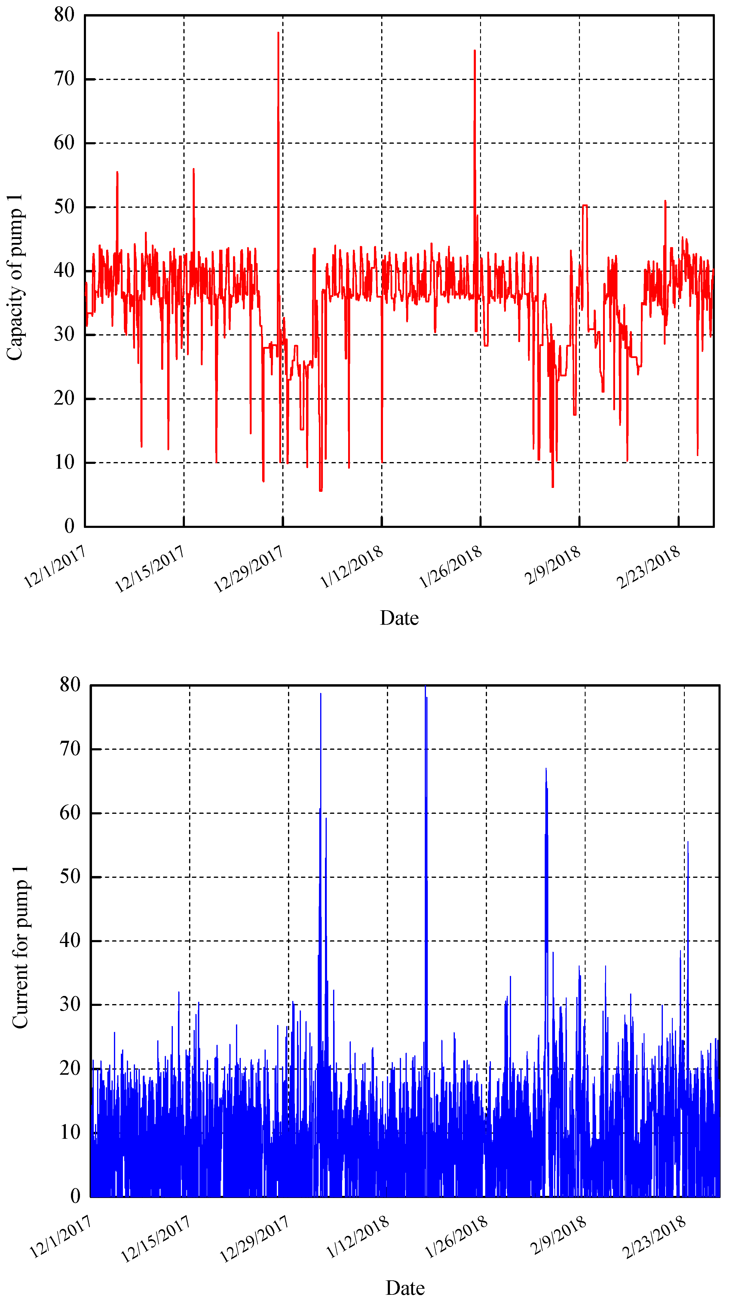
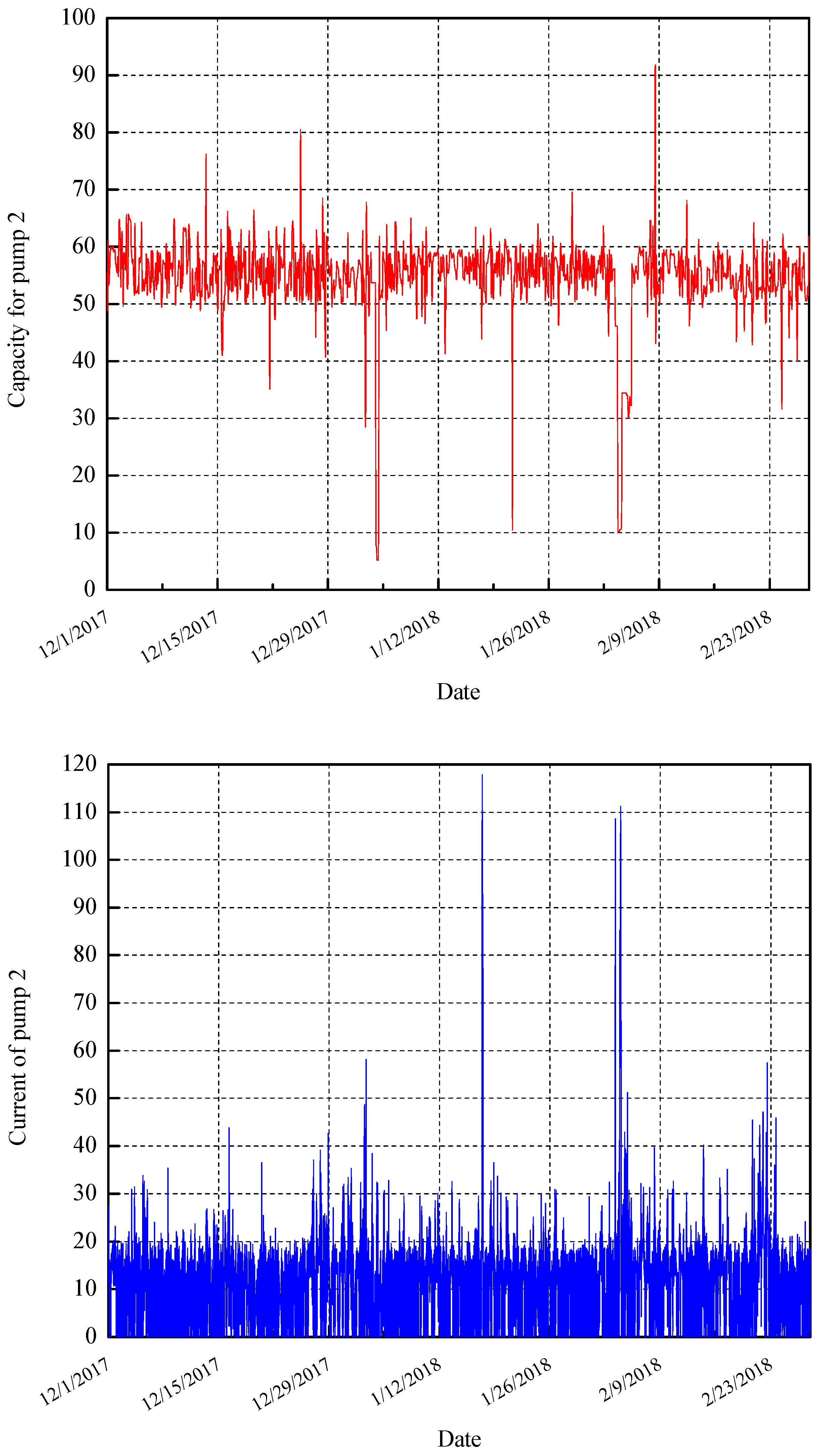
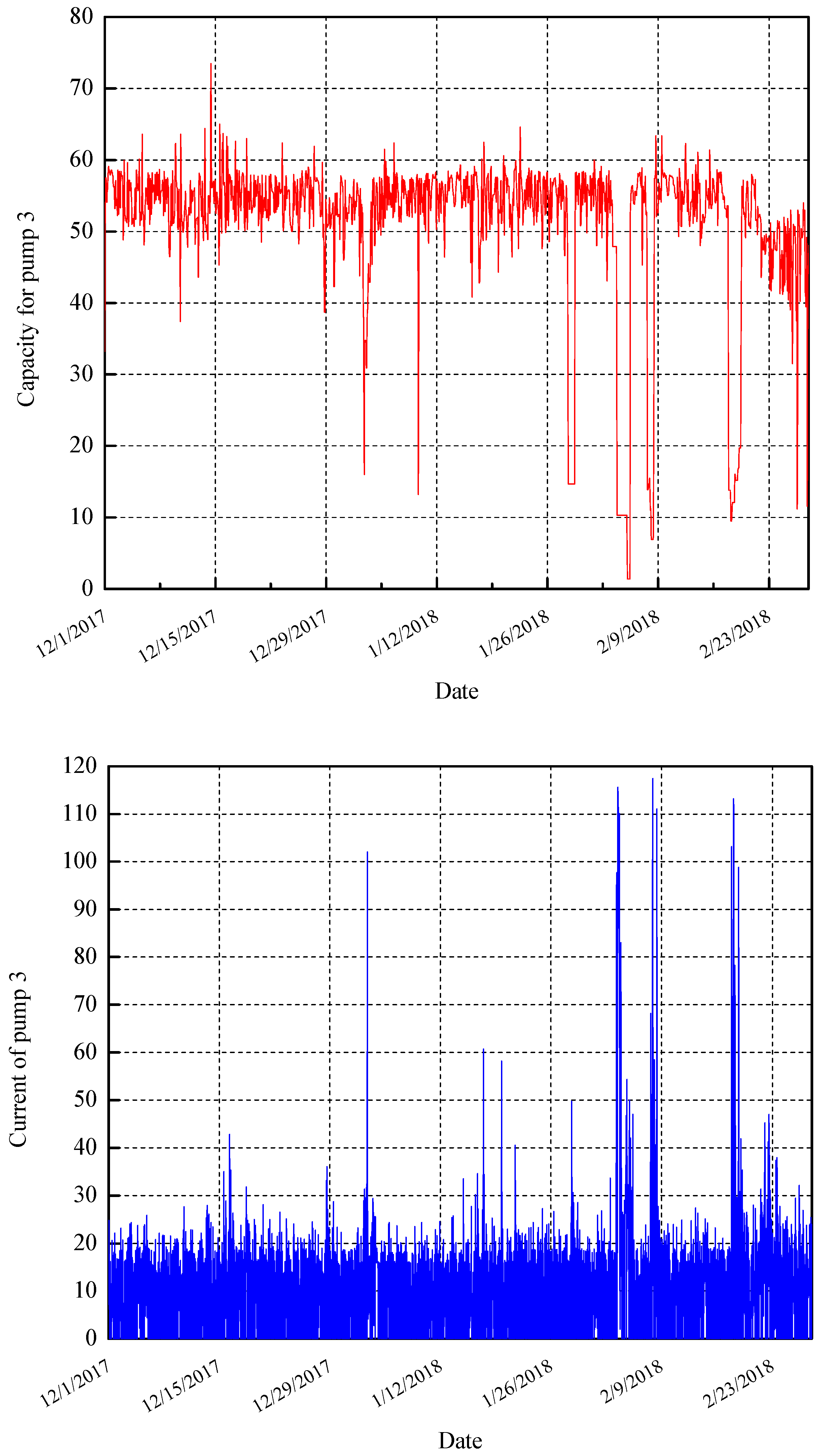
One of the particularly important functions is the reliability prediction of the working pump. Using the observed data from the process, such as the current water level in the reservoir and the inflow, the parameters of the pump, such as the value of the current and run time, can be linked and correlated to the non-electrical data. The example of these values taken from the real system are given on
Figure 1. Note that our dataset contains values of the period 2014–2019, but for a better visual representation of the data, the charts show a shorter period, i.e., the values for three months dating from 2017 to 2018.
Predictions can be made using classification or regression techniques, depending on the type of the target variable. In order to build a prediction model, an asymmetrical type dataset containing the variables was formed. Because of the difference between the variables in terms of time of measurements, all data were averaged in hours. Rows containing missing values were removed during the preprocessing phase, as well as the date and time column.
The input variables included pump capacity, current, high current, low current, nominal current, nominal capacity, inflow, lev1 value, run time and start count. The output variable was binary with two classes that were not symmetric—class zero representing the negative cases, i.e., no alarm, and class one representing positive cases, i.e., alarm (no matter if it was for high current levels, low current levels or a trip alarm). If an imbalance exists during the preprocessing phase, training data should be transformed using the combination of under sampling and oversampling techniques.
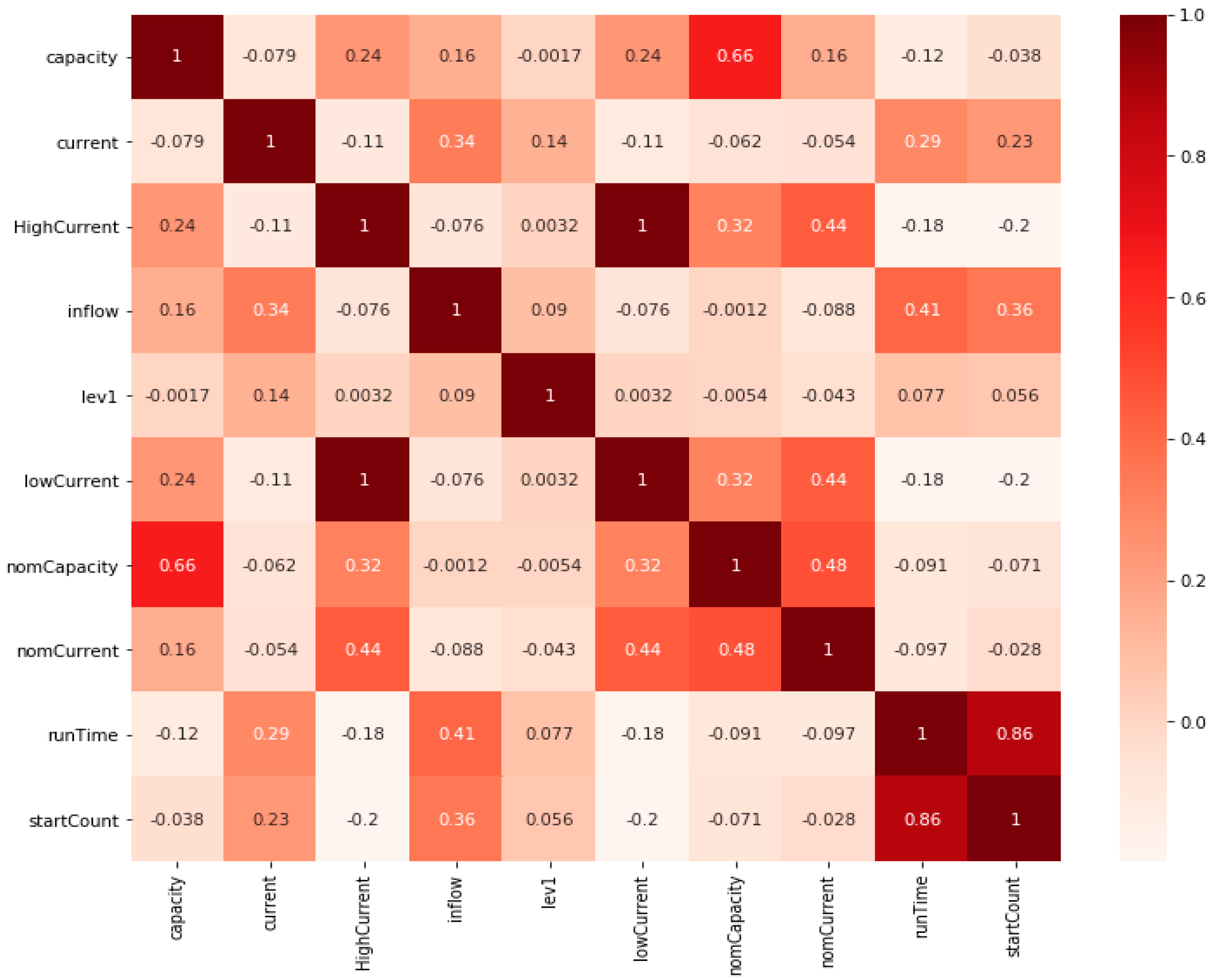
Before any simulation, a correlation matrix should be generated in order to observe the relationship between the variables. If the output variable is binary, it will not be the object of the correlation test. Correlation can provide some valuable insights into the relationships between the independent variables and can be calculated using Pearson’s correlation coefficient. Pearson’s correlation coefficient can be positive and negative and ranges from −1 to 1, where values closer to zero indicate no relationship between the observed variables, and values closer to ±1 indicate a strong relationship between the variables. The example of the correlation matrix for the sewage pump system with 10 variables is given on
Figure 2.
3. Classification Algorithms
This study used machine learning algorithms to address its aims and compares four classification algorithms: multilayer perceptron (MLP), gradient boosting trees (GBT), K-Nearest Neighbors (KNN) and random forest (RF). The study performed binary classification tasks for predicting the failure of water pumps. As training machine learning models require a careful selection of hyperparameters, this study utilized parameter estimation techniques to find the best set of parameters for our models.
3.1. Multilayer Perceptron (MLP)
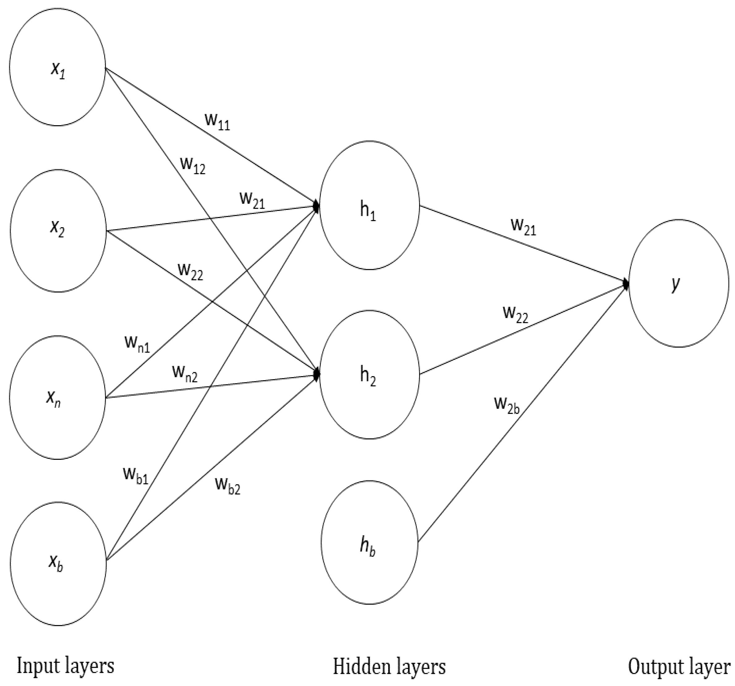
Artificial neural networks are motivated by the biological neural system. The biological neural system is composed of a large number of neurons which serve as a “processing unit”, if we consider it from the computer system’s perspective. The neurons in the brain are connected through synapses. In the same manner, artificial neural networks are composed of layers where each layer contains a number of neurons which are connected by synapses. Hence, the ANN consists of an input layer, one or more hidden layers and an output layer. The nodes from the preceding layer are interconnected to the nodes of the adjacent layer. The strength of the connection is represented through synaptic weights which present the degree of correlation between neurons. In classification, the output layer always contains that many nodes as there are classes. The MLP is presented in
Figure 3.
The MLP can be expressed as in [
15]:
thus, based on the given weights
w for input
x, the output
y can be computed. An input layer, a hidden layer and an output layer are the three layers that make up the MLP. The input layer has the task of standardizing the vector of predictor variable values in the range −1 to 1 and distributing them to each of the neurons in the hidden layer. Additionally, into each of the neurons in the hidden layer, a bias is fed, whose value is always 1.0, and a weight is multiplied by the bias and added to the sum going into the neuron. In the hidden layer, the combined value is obtained by summing the resulting weighted values, obtained by multiplying each input neuron by a weight. The weighted sum is fed into a transfer function after which output values are obtained which are further distributed to the output layer. The combined value in the output layer is obtained by summing the resulting weighted values obtained by multiplying a weight by the value from each hidden layer neuron. Feeding a weighted sum into a transfer function yields values that represent outputs from the network.
For the case of regression analysis with a continuous target variable, the output layer consists of one neuron that generates a single value, while in the case of classification problems it is being performed with categorical target variables and the output layer consists of N neurons that generate N values.
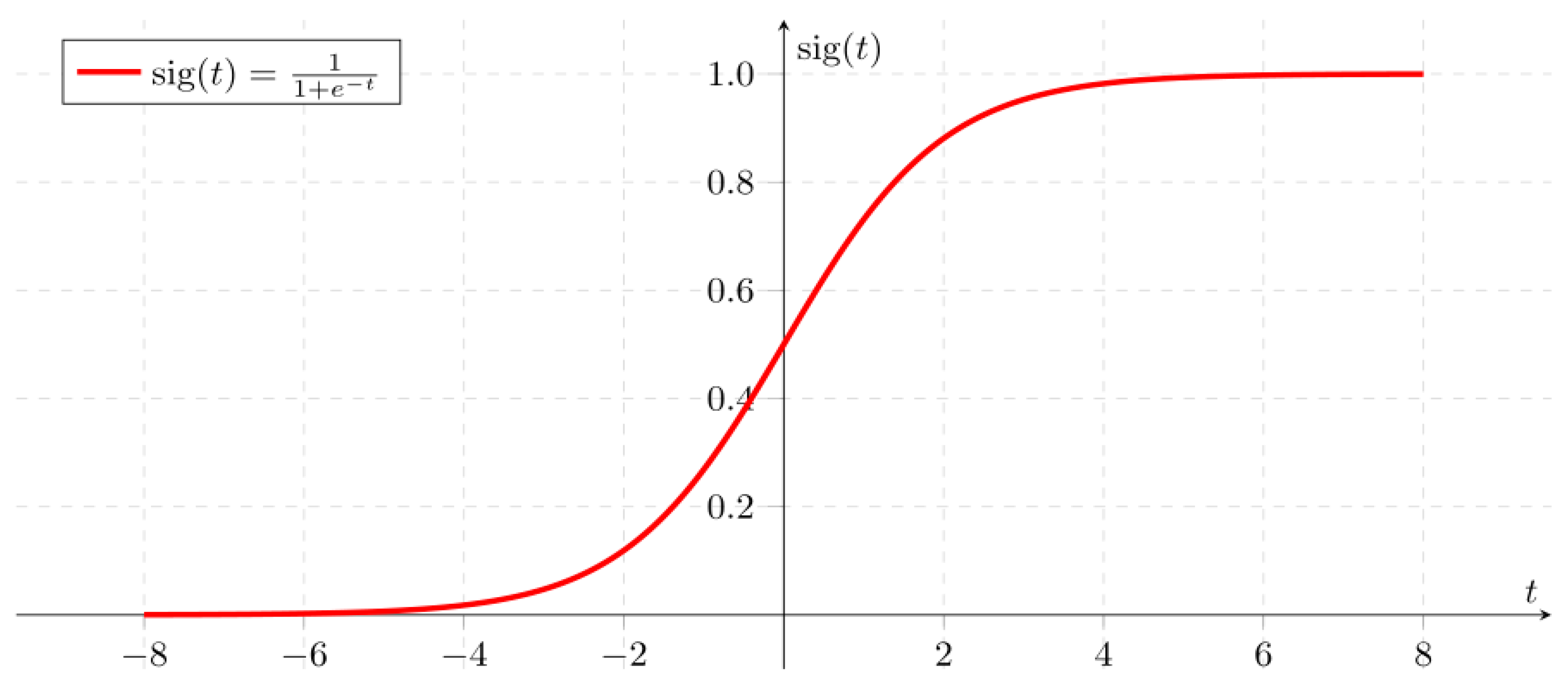
To calculate the output of the ANN, an activation function is used. From a biological perspective, the information passes inside the neuron via the action potential, which determines whether the neuron is fired or not. From the ANN perspective, the activation function determines whether a neuron is activated or not. In fact, the activation function transforms the weights received from the neurons in the input layer and sends the information to the output layer. There are many types of activation functions, including rectified linear unit (ReLU), logistic (sigmoid), binary step activation function, hyperbolic tangent (tanh), softmax and others. This study utilized the logistic (sigmoid) function, as proposed by the parameter estimation algorithm. The logistic (sigmoid) activation function is a non-linear, monotonic function and can be represented as:
The sigmoid function is an S-shaped curve (
Figure 4).
To map the real values to the predictions, neural networks use optimization (loss) functions. For these purposes, our study employed an Adam (adaptive moment estimation) optimizer. It was first presented in [
16] and it combines momentum and root mean square propagation (RMSProp) to converge faster. Momentum uses the gradients of the past and current steps to determine its direction, while RMSProp chooses a different learning rate for each parameter.
3.2. Random Forest (RF)
RFs belong to the group of ensemble learning methods where a multiple number of classifiers is generated and their results are aggregated [
17]. The algorithm was proposed in 2001 by L. Brainman [
18] and has since then demonstrated good performance for classification and regression tasks in various domains. The RF is a decision tree algorithm and is based on bagging where each tree is constructed using a different bootstrap sample, and the node is split using the best subset of randomly chosen predictors at that node [
18]. The RF performs in several steps. First, it extracts
n bootstrap samples from the asymmetrical type dataset. Then, for each of the
n bootstrap samples, an unpruned (fully grown) classification tree is developed. Finally, the prediction of new datapoints is made by majority voting of the predictions of all trees [
17].
Decision trees split the data in a way so that the largest information gain is acquired. The information gain identifies the most important feature, i.e., the feature that is most useful for making predictions. That feature is then used at the root node. Information gain is inversely related to the probability of occurrence of the observed event [
19] and can be represented as [
20]:
where
pi represents the probability of class
i.
Two common measures of impurity are the entropy and Gini indexes. Entropy can be represented as [
20]:
while Gini index can be calculated as:
If all samples of a node belong to the same class, then the entropy equals zero. For binary classification problems, the maximum entropy is one, i.e., [
20]:
This study uses entropy as an information gain criterion, which will be further explained in the next section of this paper.
3.3. Gradient Boosting Trees (GBT)
GBT are decision trees used for classification and regression problems. This algorithm performs optimization of a cost function by sequentially combining weak learners. Weak learners always perform little better than chance with errors below 0.5. The main idea behind GBT is that each new tree should minimize the cost function until there is no improvement. As opposed to RF which uses bagging, the GBT uses boosting. The algorithm assigns the same weight to each sample and then uses the first sample to train the first weak classifier [
21]. The second weak classifier is built by assigning higher weights to the misclassified samples, while lower weights are assigned to samples that were correctly classified by the first weak classifier [
21]. Finally, the classifiers are combined in one final model.
The quality of the split in this study is measured using the mean squared error (MSE) with improvement scores by Friedman. Furthermore, the GBT model was aimed to minimize the deviance loss function which can be expressed as [
22]:
where
xi is the input,
yi is the output and
f(
xi) is the function of
xi.
Boosting algorithms have been found to obtain good performances in many different areas, but it should be noted that a large feature space increases the training time [
23].
3.4. K-Nearest Neighbors (KNN)
KNN is a simple lazy algorithm developed by Thomas Cover [
24,
25] and is based on a similarity (distance) measure. The algorithm is “lazy” because it uses the training data in the testing phase, which is computationally more efficient. The KNN first calculates the distance between the d-dimensional feature vectors, and then performs classification [
26]. Even though KNN is fairly simple to use, its performance is highly impacted by the number of neighbors
k, and the selected distance measure [
27]. Different similarity measures exist, including Euclidean distance, Minkowski distance and Manhattan distance, but this study used the Manhattan distance, as proposed by the parameter estimation algorithm.
The Manhattan distance (otherwise known as city block distance) can be calculated using the sum of the absolute difference between real vectors as follows:
where
xi is the
i-th element of vector
x,
yi is the
i-th element of vector
y in the two-dimensional vector space and
n is the number of elements in the vector. Manhattan distance demonstrated good performance in the literature comparing to other distance measures. For example, in [
28] it was showed that the Manhattan distance outperforms Chebyshev and Euclidean metrics on intrusion data. Good performance of the Manhattan distance was also demonstrated in [
29,
30].
4. Results
4.1. Data Preprocessing
The dataset used in this study consisted of sensor asymmetrical type data from three water pumps. The input variables included pump capacity, current, high current, low current, nominal current, nominal capacity, inflow, lev1 value, run time and start count for each of the three water pumps. The output variable was binary with two classes—class one representing the negative cases, i.e., no alarm, and class two representing positive cases, i.e., alarm occurrence (no matter if it was for high current levels, low current levels or a trip alarm). As the sensors collected data in different time intervals, all variables were averaged on an hour level prior to modeling. All numerical results presented in this paper are based on the dataset that includes the measurements from three pumps—pump 1, pump 2 and pump 3, initially containing over 28.000 measurements. Missing values were removed before modeling, hence the final asymmetrical type dataset comprised of 25.625 measurements (70% of the data belongs to the training set, 30% of the data belongs to the test set). The data were standardized using the StandardScaler of the scikit library. StandardScaler removes the mean and scales the data to unit variance by calculating the
z score as:
where
µ represents the mean of the training samples, and
s is the standard deviation.
Due to class imbalance (class 1 includes 24.330 cases, while class 2 includes 1295 cases), during the preprocessing phase, the training asymmetrical type data were transformed using a combination of under sampling and oversampling techniques. Under sampling is used to decrease the number of cases in the majority class. It was performed using the RandomUnderSampler technique, hence the number of cases in the majority class was reduced to two times the number of cases in the minority class. On the other hand, oversampling is used to increase the number of cases in the minority class. For this purpose, the SMOTE (synthetic minority oversampling technique) technique was used. SMOTE first randomly selects an instance
a from the minority class, after which it finds the nearest neighbors and randomly chooses one and connects it to the instance
a. After performing under sampling and oversampling, both classes contained 1818 cases (
Table 1).
Each machine learning model used 70% of the data for training, and the rest for testing. Parameter estimation was performed using the RandomizedSearch CV (RS-CV), while the performance of the parameter search algorithm was evaluated using StratifiedKFold cross-validation with 10 folds.
4.2. Parameter Estimation
The models were developed after investigating the best set of parameters. For the
MLP, the activation function, solver, alpha value, batch size, and the size of the hidden layers were examined using the RS-CV (
Table 2).
The estimator suggested using the logistic activation function and one hidden layer with 96 neurons, while the weight optimization should be performed using the stochastic gradient-based optimizer (i.e., Adam). The suggested batch size was 64, while the regularization term alpha (i.e., L2 penalty) was 1 × 10⁻⁵.
The RS-CV for the GBT parameter estimation investigated the number of boosting stages (n_estimators), maximum depth of each individual estimator (max_depth), the minimum number of samples that are used to split an internal node (min_samples_split), and the minimum number of samples that are used at a leaf node (min_samples_leaf). The parameter estimation suggested 450 boosting stages, the maximum depth of 20, with 55 samples used to split the internal node, and 10 samples at a leaf node (
Table 2).
The RS-CV for KNN investigated the number of neighbors, the weight function to use in prediction, and the power parameter p that determines the distance metric. In these terms 14 neighbors were suggested to be used in the KNN model, while weighting would be performed using distance weighting. Lastly, the RS-CV suggested the power parameter p should be set to one, meaning that the distance between the points would be measured using the Manhattan distance. Parameter estimation for the KNN model is presented in
Table 2.
The RS-CV for RF investigated the number of trees in the forest (i.e., n_estimators), and the function that measures the quality of the split. The RS-CV suggested developing the RF model with 100 trees, while the quality of a split is measured using information gain (
Table 2).
4.3. Model Performance and Comparison
The asymmetrical type data were modeled using classification algorithms with parameters that were proposed by the parameter estimation algorithm. Validation of the results was performed using 10-fold cross-validation, while the performance of the models was compared using the confusion matrices and performance measures such as the area under the ROC curve (AUC ROC), f1-measure, precision and recall. The metrics such as AUC ROC, precision, recall, and f1-measure were calculated on the test set. Precision is calculated as the number of correct positive predictions divided by the total number of positively predicted instances. Recall, also known as sensitivity and true positive rate, is calculated as the ratio of the number of correct positive predictions divided by the total number of positive samples. Precision, recall and accuracy can have values in range [0,1], with values closer to one indicating a better model. Finally, F-measure represents the weighted average of precision and recall.
As this is a binary classification problem with originally highly imbalanced data, accuracy measure should not be used as the main performance metric because it can generate good accuracy based on the accuracy of the majority class. Hence, we have utilized ROC AUC value as the main performance metrics. The models were also evaluated from the perspective of the time taken to estimate parameters, train and test the models.
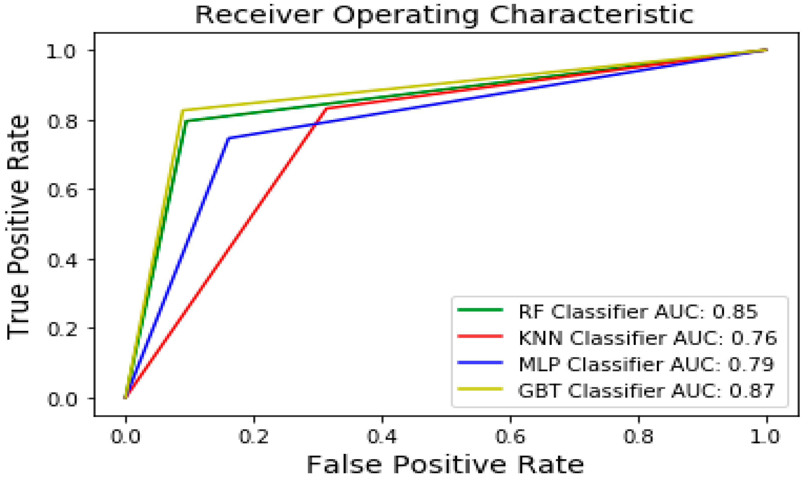
Considering validation accuracy, the best performing models were the GBT and the RF with 92.44 and 91.09% accuracy, respectively. The accuracy on the training dataset was 100% for GBT, KNN, and RF, while the MLP obtained training accuracy of 98%. The GBT and RF also obtained the best values in terms of precision, recall and f1-score. In particular, the GBT obtained 0.66 precision, 0.87 recall, and 0.71 f1-score. The RF obtained precision of 0.65, recall of 0.85 and f1-score of 0.69, indicating a good potential of classification. As the most important metric, AUC ROC scores were evaluated and compared. The highest area under the ROC was obtained for the GBT and RF classifiers, with values of 86.9 and 85.00%, respectively. The MLP classifier obtained an AUC ROC value of 79%, while KNN obtained 76%, demonstrating the weakest ability to classify water pump sensor data. These results are presented in
Table 3, followed by
Figure 5 where the AUC curves of each model are compared.
Additionally, when discussing ML models, it is important to observe the time needed to train and test the model, because it is important for the model to be less computationally intensive. The RS-CV took almost 600 s to search for the best set of parameters for the MLP model, 209 s for the GBT, 1.9 s for the KNN, and 28 s for the RF. Furthermore, it took one minute to train the MLP, 10.6 s to train the GBT, 0.03 s to train the KNN, and 11.83 to train the RF. Even though the KNN took the lowest time to search for parameters and train the model, considering other metrics the best performing algorithms were RF and GBT.
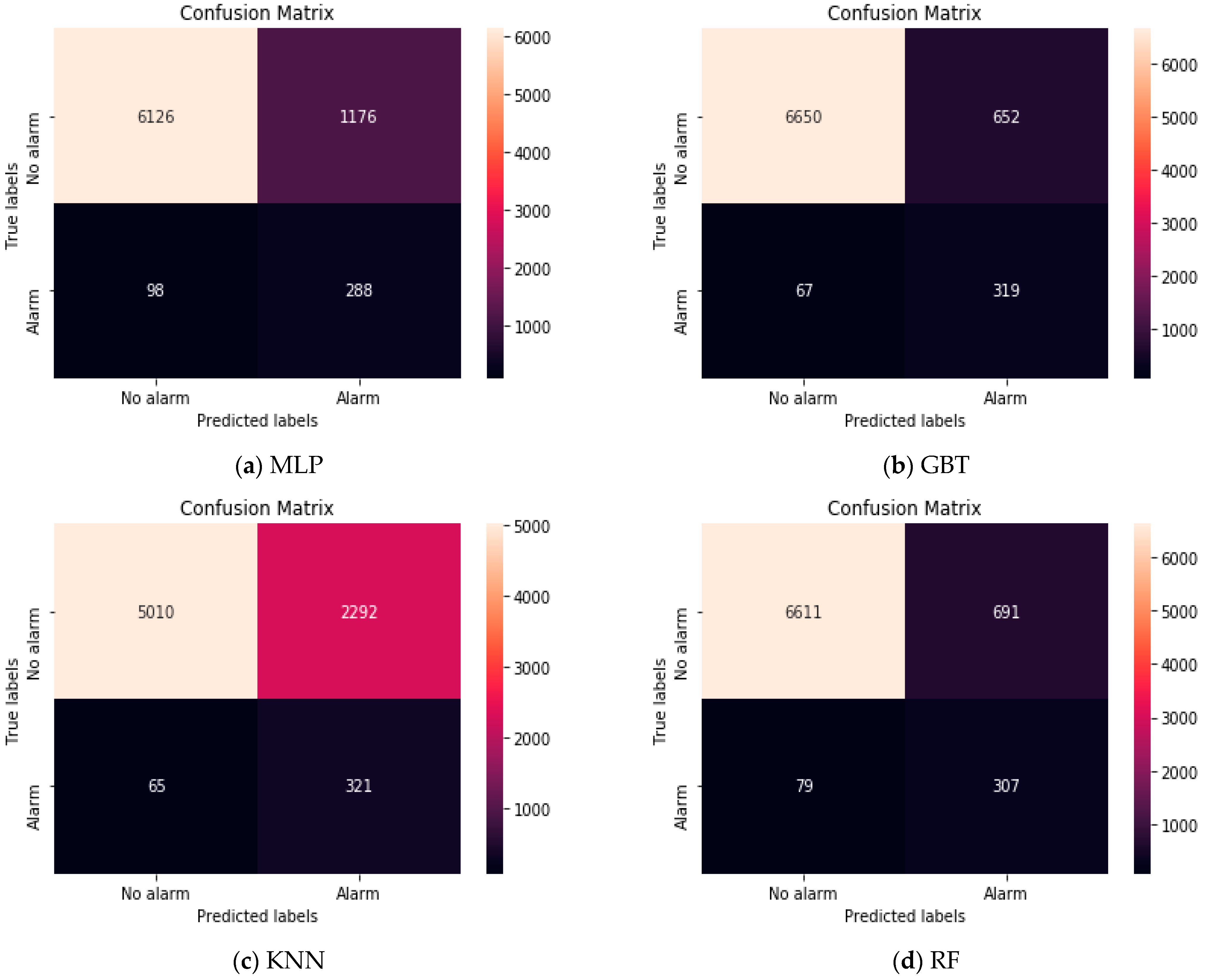
Lastly, to better understand the performance of the examined classifiers and their ability to correctly classify faults of water pumps, a 2 × 2 confusion matrix was generated. The columns show the number of predicted test samples for the negative class (no alarm) and positive class (alarm), while the rows present the true number of test samples belonging to the observed classes. On the test set, 6126 truly negative samples were correctly classified as negative (true negative) by the MLP model, while 288 truly positive samples were correctly classified as positive (true positive). There were 1176 false positive samples (samples predicted as positive but are really negative) and 98 false negative samples (predicted as negative but are actually positive). Considering that the intention was to classify pump failure, it was important to have low values of false negative samples as the consequences otherwise could be severe; if the sample was predicted as no fault, but there was really a pump failure, there would be big costs that could be avoided with on-time prediction and management. Furthermore, increasing the dataset size with samples belonging to the positive class would provide more real information to the algorithm which will increase the model performance significantly.
The GBT correctly classified 6650 truly negative samples, while 319 samples truly positive samples were correctly classified as positive. There were 652 false positive samples and 67 false negative samples. The KNN obtained the lowest performance, with 5010 correctly classified truly negative samples, 321 correctly classified truly positive samples, 2292 false positives and 65 false negatives. Lastly, the RF correctly classified 6611 negative samples and 307 positive samples, while there were 691 false positives and 79 false negatives. These results are presented in
Figure 6.
The methodology presented in the past section can be used for the prediction of pump failure or alarm states. Additionally, the minimum and maximum values for each variable when the observed alarm occurred were inspected. In particular, we see that for pump 1, the high current alarm occurred when the capacity of the pump 1 had the values between 45.8 and 54, while the current had the values between 14.57 and 24.99. The high current values were between 100 and 199, while the inflow value was in the range [10.42, 19.45]. Similar results can be observed for the rest of the variables as well, but also for the low current alarm and the trip alarm for all three pumps. It is essential to mention that these values represent the average hourly values.
The obtained results demonstrate good performance and are in line with some of the findings from the literature. In particular, a study by [
12] detected faults in large water networks through online dictionary learning. The results of the proposed methodology were compared to the KNN and SVM algorithms and demonstrated that KNN and support vector machines (SVM) perform better with a small number of sensors, while online dictionary learning was better suited for large values [
31]. Failure in mechatronic water plant system was modeled in [
32] using the KNN, Logistic regression (LR) and SVM algorithms. The performance was examined on the full dataset containing 51 attributes, and on the reduced set with 22 attributes. The highest accuracy on both the full dataset and the reduced set was obtained by the KNN—98.9 and 99.97%, respectively, demonstrating good performance of the KNN for sensor data [
32].
5. Conclusions
Based on the obtained results, it can be concluded that ML algorithms can be successfully used for predicting water pump failure. In order to generate more detailed and correct predictions, it is important to have more data, especially data of alarm cases, which will increase the distribution of this class and provide more information to the algorithm, thus obtaining more accurate prediction.
Predictions of pump failures suggest some interesting findings. In the first place, the random forest classification technique can be successfully utilized to classify sensor data. The model is appropriate for fine-tuning, but it also improves its performance over time. Furthermore, the developed models suggest that the performance significantly improves with bigger number of real values in the minority class. Even though sampling techniques (such as under sampling and oversampling) fix the issue of class imbalance, the model is able to learn much better on real-world data, hence with large enough number of cases in the minority class, the predictions are certainly more accurate.
The goal of future work is to improve the considered algorithms by forming as large as possible databases of all data that make up the model in order to increase the accuracy of prediction. Additionally, the goal of future work is that by applying the considered algorithms, the system identifies patterns and helps to make more accurate decisions regarding network resilience, energy efficiency, wastewater minimization, cost reduction etc. Further development of this solution will optimize water distribution systems, their infrastructure, operations, monitoring, maintenance and management.


