A Multichannel Data Fusion Method Based on Multiple Deep Belief Networks for Intelligent Fault Diagnosis of Main Reducer

Abstract

Aiming at the problems of poor efficiency of the intelligent fault diagnosis method of the main reducer and the poor effectiveness of multichannel data fusion, this paper proposes a multichannel data fusion method based on deep belief networks and random forest fusion for fault diagnosis. Multiple deep belief networks (MDBNs) are constructed to obtain deep representative features from multiple modalities of multichannel data. Random forest can fuse deep representative features achieved from MDBNs to construct the model of multiple deep belief networks fusion (MDBNF). The proposed method is applied to fault diagnosis of the main reducer and evaluation of the performance. Multiple deep belief network model fusions (MD BN F) are constructed to improve the multichannel data fusion effect. Single sensory data, multichannel data, and two intelligent models based on support vector machine and deep belief networks are used as comparison in the experiments. The results indicate that the classification accuracy of the test set collected by sensor 1 and sensor 2 is 88.35% and 88.73%, respectively. The comparison results show that the method has good convergence. The data fusion of the proposed diagnostic model can effectively improve the correlation between the collected vibration signals and the failure mode, thereby improving the diagnostic performance by nearly 8%, representing improved diagnostic accuracy.

1. Introduction

As the crucial part of the rear axle, the condition of the main reducer has a direct impact on the level of vibration, safety and comfort, and any fault of the main reducer may lead to production downtime, economic loss and human injury [1,2]. Vibration signals generated during the running process can effectively reflect the variance of condition. Therefore, fault diagnosis based on vibration signals is the most-used way of machinery condition monitoring and fault diagnosis [3]. McLaughlin et al. utilized bi-spectrum analysis based on modulating signal to acquire features of gear vibration signal [4]. Marnatha et al. employed vibration signals and statistical parameters to detect local fault of helical gear tooth [5]. Yang et al. employed ensemble empirical mode decomposition to extract features of gear vibration signals [6]. Jena et al. used active noise cancellation and adaptive wavelet transform in gear fault diagnosis [7].

The first step of machinery fault diagnosis is to monitor valid condition symptom [8,9]. Due to the configuration complexity and failure diversity of mechanical system, it’s difficult to determine the best position of sensors for monitoring. Meanwhile, the relationship between fault patterns and condition symptoms is complex and non-linear mapping [10]. Collecting vibration signals from single-channel sensors may encounter the limitations of installation position and direction of sensor so as to decrease the diagnostic accuracy [11,12]. Based on this, it is necessary to employ multiple sensors along different transmission paths to collect multichannel vibration signals. However, fault diagnosis based on multichannel data suffers from two challenges. Firstly, due to the heterogenicity of multichannel data, using traditional shallow structure to extract features from multiple types of sensory data will decrease the diagnostic accuracy [13,14]. Secondly, how to effectively fuse the features extracted from multichannel data is another challenge [15].

Due to the complicated running environment, the collected condition symptom is always interfered by paroxysmal noise and vibration disturbance originated by other components and obstacles [16]. The second step of fault diagnosis is to achieve deep representative features which are sensitive to fault patterns from multichannel vibration signals. Recently, deep learning is widely used to extract fault-sensitive features from statistical parameters for fault diagnosis using deep structure [17,18]. Tamilselvan et al. used deep learning to implement health state classification [19]. Feng et al. employed deep neural networks to mine characteristic of rotating machinery with massive data [20].

Deep representative features extracted from multichannel data represent multiple modalities of raw vibration signals, and may lead to different fault-sensitivity of these modalities of features [21]. The third step of fault diagnosis is to fuse deep representative features of multiple modalities from multichannel data and obtain the final diagnostic result. The most-used fusion methods include K-nearest-neighbor (KNN), support vector classification (SVC) and random forest [22]. Li et al. used supervised bounded component analysis to detect gear cracks of wind turbines with vibration signals collected from multichannel sensors [11]. Duro et al. proposed a multi-sensor data fusion framework for machine monitoring [12].

Aiming to solve the challengers of fault diagnosis based on multichannel data, this paper proposes a multichannel data fusion method based on multiple deep belief networks (MDBNs) and random forest fusion for fault diagnosis. Firstly, multichannel vibration signals are collected using multiple sensors to implement reliable monitoring. Secondly, multiple modalities features are extracted from multichannel data using different preprocessing techniques. Then, MDBNs are constructed to obtain deep representative features from multiple modalities of multichannel data. Finally, we fuse deep features form MDBNs using random forest to construct the model of multiple deep belief networks fusion (MDBNF).

The rest of the paper is organized as follows: the deep learning and fusion of deep representative features from multichannel data is presented in Section 2; application of intelligent fault diagnosis for the main reducer is presented in Section 3; in Section 4, fault diagnosis experiments of the main reducer are carried out to evaluate the efficiency of the proposed method; finally, conclusions are addressed in Section 5.

2. Deep Learning and Fusion of Deep Representative Features

2.1. Deep Belief Networkwith Gaussian-Bernoulli RBM

A deep belief network (DBN) is a typical form of deep learning network and contains a visible layer, multiple hidden layers and an output layer. The visible layer is used to input data and then transmit data through hidden layers to achieve non-linear transform as the process of deep learning [20,21]. 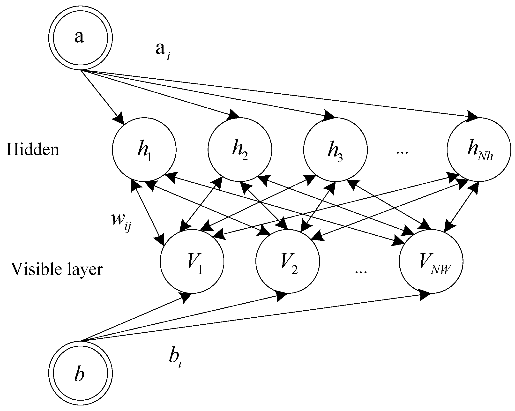The structure of DBN is a stack of restricted Boltzmann machines (RBMs), which is composed of a visible layer and a hidden layer with binary stochastic units [22]. In order to deal with real-valued input data that can’t be normalized into {0, 1}, we propose to use Gaussian-Bernoulli RBM (GRBM) [23] in which the visible units are Gaussian neurons to constitute DBN. The architecture of GRBM is shown in Figure 1.

In Figure 1, Vi and hi ∈ {0,1} are visible units and hidden units. Vector a and b represent the biases of hidden layer and visible layer, wij represents weight between the ith visible unit and the jth hidden unit. N_v and N_h separately represent the number of visible units and hidden units. Considering the standard deviation of visible units, the joint energy of visible and hidden layer units of GRBM is given as follows:

$$E\left(\mathrm{v},\mathrm{h};\theta \right)={\displaystyle \sum }_{i=1}^{N_v}\frac{{\left(V_i-b_i\right)}^2}{2{\sigma }^2}-{\displaystyle \sum }_{j=1}^{N_h}{a}_j{h}_j-{\displaystyle \sum }_{i=1}^{N_v}{\displaystyle \sum }_{j=1}^{N_h}\frac{V_i}{{\sigma }_i}{w}_{ij}{h}_j$$

(1)

where $\theta =\left\{\mathrm{w},\mathrm{b},\mathrm{a}\right\}$ are the model parameters and ${\sigma }_i$ represents the standard deviation of the ith visible unit. The joint probability distribution of visible vector $\mathrm{v}$ and hidden vector $\mathrm{h}$ is defined as follows:

$$P\left(\mathrm{v},\mathrm{h};\theta \right)=\frac{1}{Z\left(\theta \right)}\exp \left(-E\left(v,h;\theta \right)\right)$$

(2)

$$Z\left(\theta \right)={\displaystyle \sum }_{\mathrm{V}}{\displaystyle \sum }_{\mathrm{h}}\exp \left(-E\left(\mathrm{v},\mathrm{h};\theta \right)\right)$$

(3)

where $Z\left(\theta \right)$ is the normalization factor, which depends on $\theta$. For a specific GRBM structure without interlayer connections, the visible vector $\mathrm{v}$ and hidden vector $\mathrm{h}$ are conditional independent. The probabilities of visible vector $\mathrm{v}$ can be given:

$$P\left(\mathrm{v};\theta \right)=\frac{1}{Z\left(\theta \right)}\exp (\frac{{\left(\mathrm{b}-\mathrm{v}\right)}^T\left(\mathrm{b}-\mathrm{v}\right)}{2{\sigma }^2}){\displaystyle \prod }_{j=1}^{N_h}(1+\exp (a_j+{\displaystyle \sum }_{i=1}^{N_v}{w}_{ij}\frac{V_i}{{\sigma }_i}))$$

(4)

The conditional probabilities of the ith visible unit $V_i$ and the jth hidden unit $h_j$ are expressed as follows:

$$P\left(V_i=x|\mathrm{h};\theta \right)=\frac{1}{{\sigma }_i\sqrt{2\pi }}\exp (-\frac{{(x-b_i-{\sigma }_i{{\displaystyle \sum }}_j{h}_j{w}_{ij})}^2}{2{\sigma }^2})$$

(5)

$$P\left(h_j=1|\mathrm{v};\theta \right)=\mathrm{g}\left(a_j+{\displaystyle \sum }_i{w}_{ij}\frac{v_i}{{\sigma }_i}\right)$$

(6)

where $x$ is a real number and $\mathrm{g}\left(·\right)$ represents the logistic function.

By stacking L GRBMs, a DBN is constructed with L hidden layers (h⁽¹⁾, h⁽²⁾,…, h^(L)) in which input layer and h⁽¹⁾ form GRBM1, h⁽¹⁾ and h⁽²⁾ form GRBM2, h^(L−1) and h^(L) form GRBM L.

The training of the DBN consists of two procedures: pretraining and fine-tuning [24]. The first procedure is unsupervised pretraining of a stack of GRBMs one-by-one. The lower layer of each GRBM is used as the input layer of next GRBM and the parameters containing weight and biases of each GRBM are optimized independently. Once the previous GRBM finishes the pretraining, the next GRBM starts pretraining. The second procedure is supervised fine-tuning of the whole networks by back propagation algorithm. In this procedure, all of the hidden layers are considered as a whole and model parameters are adjusted to decrease the training error [25].

2.2. Deep Learning of Multichannel Data Using MDBNs

Through several nonlinear transformations in the form of a stack of GRBMs, a DBN can effectively extract the deep representative features. In order to obtain reliable data to ensure diagnostic accuracy, we propose to use multiple sensors to collect multichannel vibration signals as the input data of diagnostic model.

Srivastava et al. proposed a multimodal learning method with deep Boltzmann machines by direct combination of multiple modalities [26]. However, the calculation cost of direct linear combination of input data with different modalities is too high, and the execution time will be increased. The combination process may occupy a large memory space and bring contradictions and conflicts [27]. Based on this, we construct multiple deep belief networks (MDBNs) in which each DBN is used to obtain deep representative features of vibration signal collected from one channel.

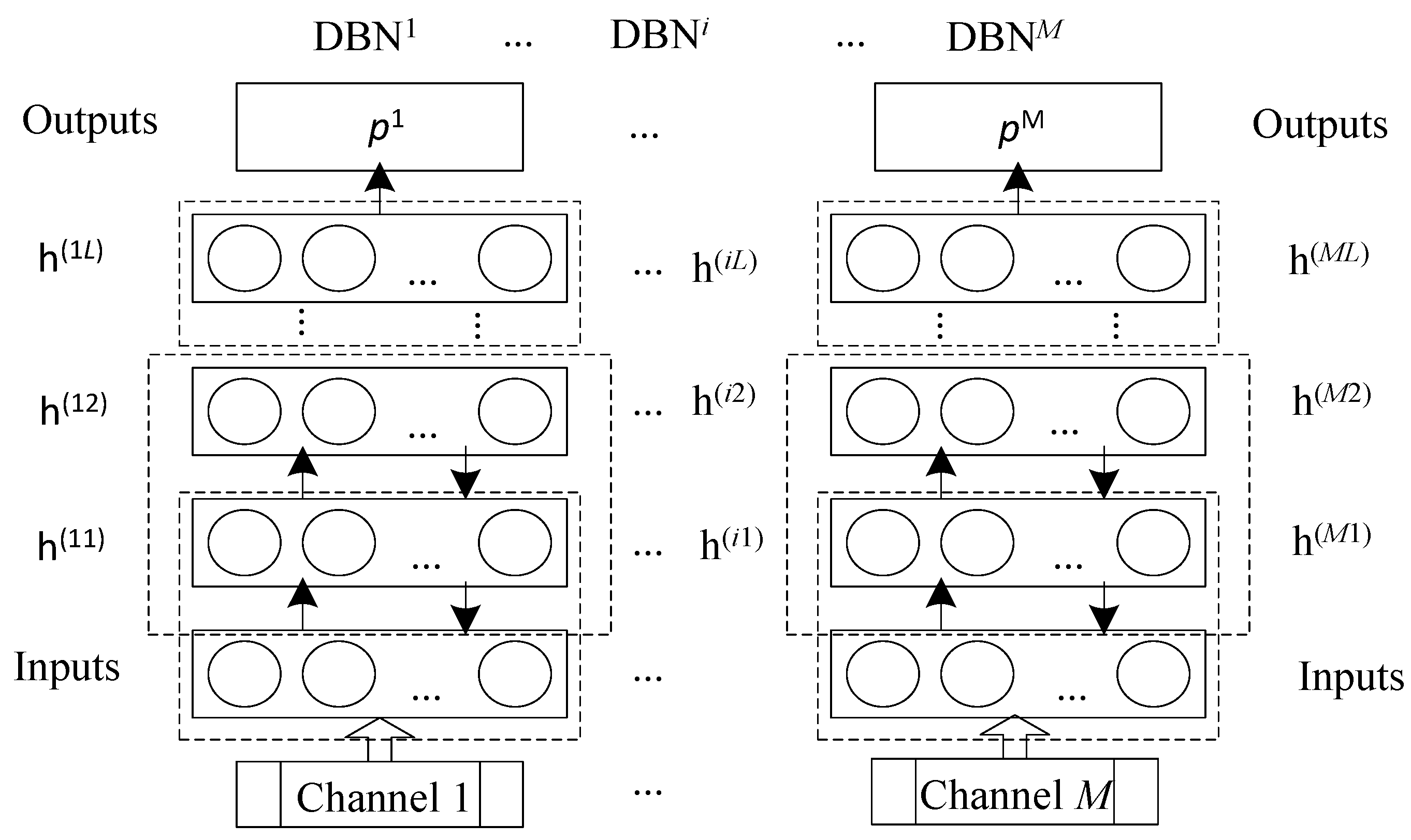
As shown in Figure 2, the architecture of MDBNs consists of several structures of DBNs (expressed as DBN¹, DBN²,…, DBN^M) wherein DBNⁱ is used to learn deep representative features of the vibration signals collected from the ith channel of M channels expressed as Channel 1, Channel 2,…, Channel M. By using MDBNs, after multiple non-linear hierarchical transformations of the input data from multichannel, the deep representative features of the raw data are acquired.

With the input data of multichannel represented as X⁽¹⁾, X⁽²⁾,…, X^(M), the output of the ith DBN is expressed as:

$$p^i=\left(p_1^{\left(i\right)},p_2^{\left(i\right)},\dots ,p_{{\mathrm{N}}_{iL}}^{\left(i\right)}\right)$$

(7)

where i=1,2,…, M and ${\mathrm{N}}_{iL}$ represents the number of the output units of the ith DBN. With the proposed MDBNs, each channel data X⁽ⁱ⁾ is converted into deep representative features expressed as $p^i$.

In order to obtain final diagnostic result, the output vector $\left(p^1,p^2,\dots ,p^M\right)$ of MDBNs with M independent DBN structure needs to be used as the input of the diagnostic model. The output vector of MDBNs is expressed as follows:

$$\left(p^1,p^2,\dots ,p^M\right)=\left(p_1^{\left(1\right)},\dots ,p_{{\mathrm{N}}_{1L}}^{\left(1\right)},\dots , p_1^{\left(i\right)},\dots ,p_{{\mathrm{N}}_{iL}}^{\left(i\right)},\dots , p_1^{\left(M\right)},\dots ,p_{{\mathrm{N}}_{ML}}^{\left(M\right)}\right)$$

(8)

2.3. Random Forest Fusion of Deep Representative Features

With the representative features of each DBN in the form of Equation (7), diagnostic model could acquire a result $f^i$ as condition pattern corresponding to the vibration signal collected from the ith channel. However, results of multiple DBNs corresponding to multichannel vibration signals may be contradictory, such as: $f^i\ne f^j$. The difficulty comes in determining which DBN’s result is valid. Therefore, we fuse the output of each DBN together to form the input of diagnostic model.

In order to effectively fuse deep representative features in the form of Equation (8) extracted from multichannel vibration signals by using MDBNs, we propose to use random forest to fuse these features and achieve the final result. By using the fusion strategy, we can obtain the final result expressed as follows:

$$f=\mathrm{F}\left(p_1^{\left(1\right)},p_2^{\left(1\right)},\dots ,p_{{\mathrm{N}}_{1L}}^{\left(1\right)},\dots , p_1^{\left(i\right)},p_2^{\left(i\right)},\dots ,p_{{\mathrm{N}}_{iL}}^{\left(i\right)},\dots , p_1^{\left(M\right)},p_2^{\left(M\right)},\dots ,p_{{\mathrm{N}}_{ML}}^{\left(M\right)}\right)$$

(9)

where $\mathrm{F}\left(·\right)$ represents the fusion function.

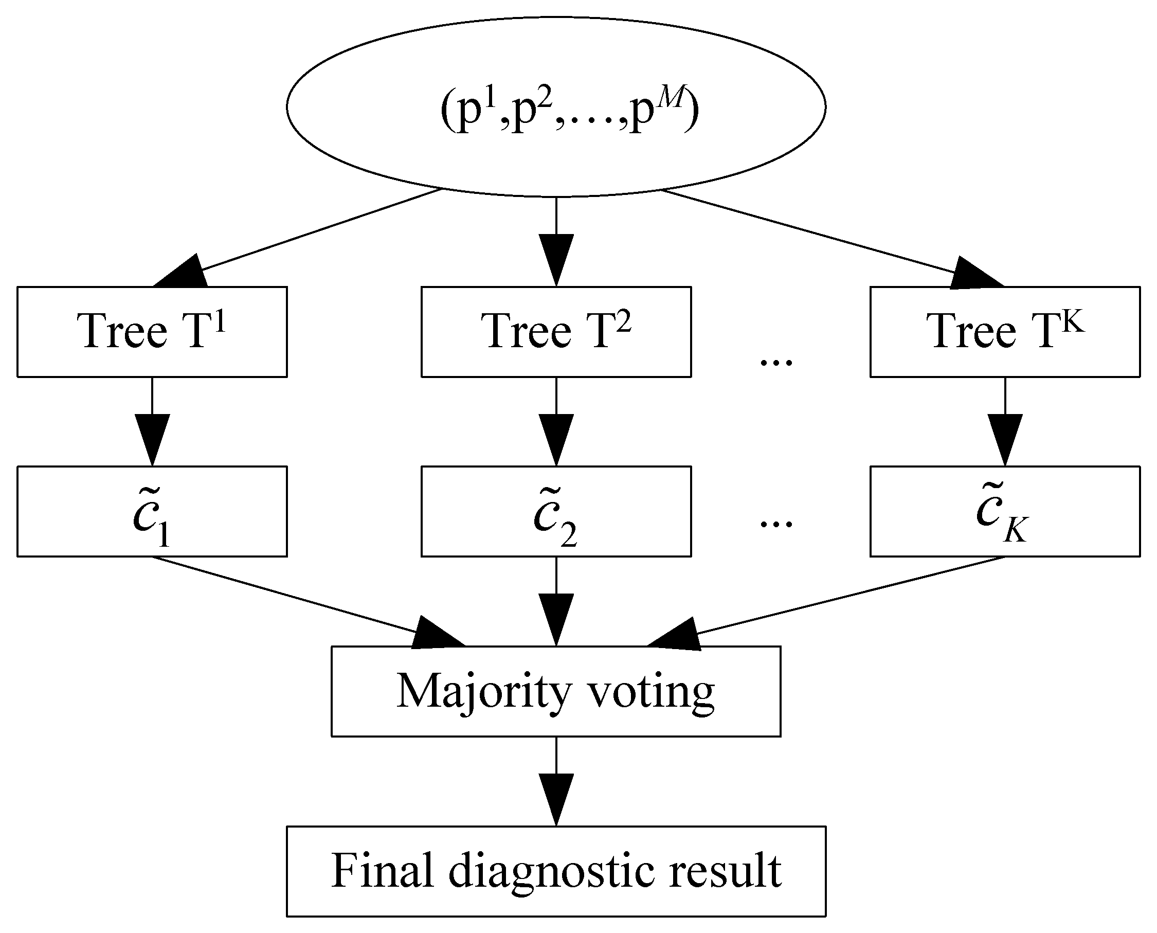
As shown in Figure 3, the fusion model based on random forest consists of K decision trees expressed as $\{{\mathrm{T}}^1,{\mathrm{T}}^2\dots ,{\mathrm{T}}^K\}$ with the output of K decision trees as the diagnostic results. Each decision tree is composed of several splits and nodes in which splits lead the direction of output and nodes determine the output of this decision tree in the form of a specific class $\tilde{c}$. The output of K decision trees is generated to codetermine the output vector of the fusion model expressed as follows:

$$\mathrm{C}=\left\{\widetilde{c_1},\dots ,\widetilde{c_k},\dots ,\widetilde{c_K}\right\}$$

(10)

where $\widetilde{c_k}$ is the class assigned by the kth decision tree ${\mathrm{T}}^k$. With the output vector $\mathrm{C}$, the final diagnostic result is produced by majority voting operation:

$$f=majorityvote{\left\{\widetilde{c_1},\dots ,\widetilde{c_k},\dots \widetilde{c_K}\right\}}_1^K$$

(11)

3. Application to Intelligent Fault Diagnosis of Main Reducer

The proposed multichannel data fusion method based on multiple deep belief networks and random forest fusion is applied to construct an intelligent fault diagnostic model of MDBNF. The model includes five modules: collecting multichannel vibration signal using multiple sensors, preprocessing of the collected signals to generate multiple modalities features, deep learning of multiple modalities features using MDBNs, fusion of deep representative features obtained from MDBNs, making diagnostic decision.

3.1. Multiple Modalities Features of Multichannel Vibration Signal

Multiple modalities features of multichannel vibration signal can be extracted using different preprocessing techniques, such as time domain analysis, frequency domain analysis and time-frequency domain analysis. Considering the complementarity of these techniques, we utilize all these techniques to achieve multiple modalities features of multichannel vibration signal.

Time domain analysis technique is easy to implement and independent to rotating speed. Frequency domain analysis technique is superior to time domain analysis technique for early-stage and distributed faults [28,29,30,31]. Therefore, we employ eight statistical parameters including kurtosis, crest factor, variance, standard deviation, RMS, skewness, mean and impulse indicator [32] expressed as follows to implement the preprocessing of time domain and frequency domain signals.

$$\mathrm{K}\left(x\right)=\frac{1}{n}{\displaystyle \sum }_{i=1}^n{\left(x\left(i\right)\right)}^4$$

(12)

$$\mathrm{C}\left(x\right)=\frac{\max \left|x\left(i\right)\right|}{\sqrt{\frac{1}{n}{{\displaystyle \sum }}_{i=1}^n{\left(x\left(i\right)\right)}^2}}$$

(13)

$$\mathrm{V}\left(x\right)=\frac{1}{n}{\left(x\left(i\right)\right)}^2$$

(14)

$$\mathrm{SD}\left(x\right)=\frac{1}{n}{\displaystyle \sum }_{i=1}^n\left|x\left(i\right)-\overline{x}\right|$$

(15)

$$\mathrm{R}\left(x\right)={\left(\frac{1}{n}{\displaystyle \sum }_{i=1}^n\sqrt{\left|x\left(i\right)\right|}\right)}^2$$

(16)

$$\mathrm{S}\left(x\right)=\frac{1}{n}{\left(x\left(i\right)\right)}^3$$

(17)

$${\mathrm{M}}_{\mathrm{ean}}\left(x\right)=\frac{1}{n}{\displaystyle \sum }_{i=1}^n\left|x\left(i\right)\right|$$

(18)

$$\mathrm{I}\left(x\right)=\frac{\max \left|x\left(i\right)\right|}{{\left(\frac{1}{n}{{\displaystyle \sum }}_{i=1}^n\left|x\left(i\right)\right|\right)}^2}$$

(19)

where $x\left(i\right)$ is the signal and n is the length of $x\left(i\right)$. Additionally, we use wavelet package transform (WPT) to decompose the vibration signal for time-frequency domain analysis and to extract more condition parameters. With the maximum decomposition level of J, we calculate the wavelet coefficients and use two^J energies of the Jth level as condition parameters of time-frequency domain.

In this way, multiple modalities features of vibration signal consist of eight statistical parameters of the time domain, eight statistical parameters of the frequency domain and two^J condition parameters of the time-frequency domain expressed as follows:

$$z_1=s\left(x\right)$$

(20)

$$z_2=s\left(f\left(x\right)\right)$$

(21)

$$z_3=\left[E\left(J,1\right),E\left(J,2\right),\dots ,E\left(J,2^J\right)\right]$$

(22)

where $z_1$, $z_2$ and $z_3$ separately represent parameters of time domain, frequency domain and time-frequency domain.

For multichannel vibration signal, multiple modalities features are expressed as Z = [Z¹,…,Zⁱ,…Z^M] in which Zⁱ = [z₁ⁱ,z₂ⁱ,z₃ⁱ] represents multiple modalities features of vibration signal collected from the ith sensor.

3.2. The Proposed Diagnostic Model of MDBNF

With the multiple modalities features of multichannel vibration signal in the form of multiple statistical parameters, the proposed diagnostic method constructs MDBNs model as shown in Figure 2 to obtain deep representative features of multiple modalities from multichannel data which are sensitive to fault patterns.

For each DBN in MDBNs, a greedy and layer-to-layer unsupervised learning is executed to implement non-linear mapping and model advanced abstraction of raw signal collected from each sensor. After the pretraining of DBN model, fine-tune the parameters of model in supervised way by using back-propagation algorithm to improve the diagnostic accuracy. After the unsupervised pretraining and supervised fine-tuning process, the model of DBN is well trained and generated using training samples. The output the each DBN model is a deep representative feature vector expressed as Equation (7) of one channel data.

In order to process multichannel vibration signals collected from multiple sensors, multiple DBNs constitute the model of MDBNs to obtain deep representative features of multichannel data. With the output vector of MDBNs expressed as Equation (8), a fusion model as shown in Figure 3 is constructed to fuse the multiple modalities of deep representative features, and then make the diagnostic decision using Equation (11).

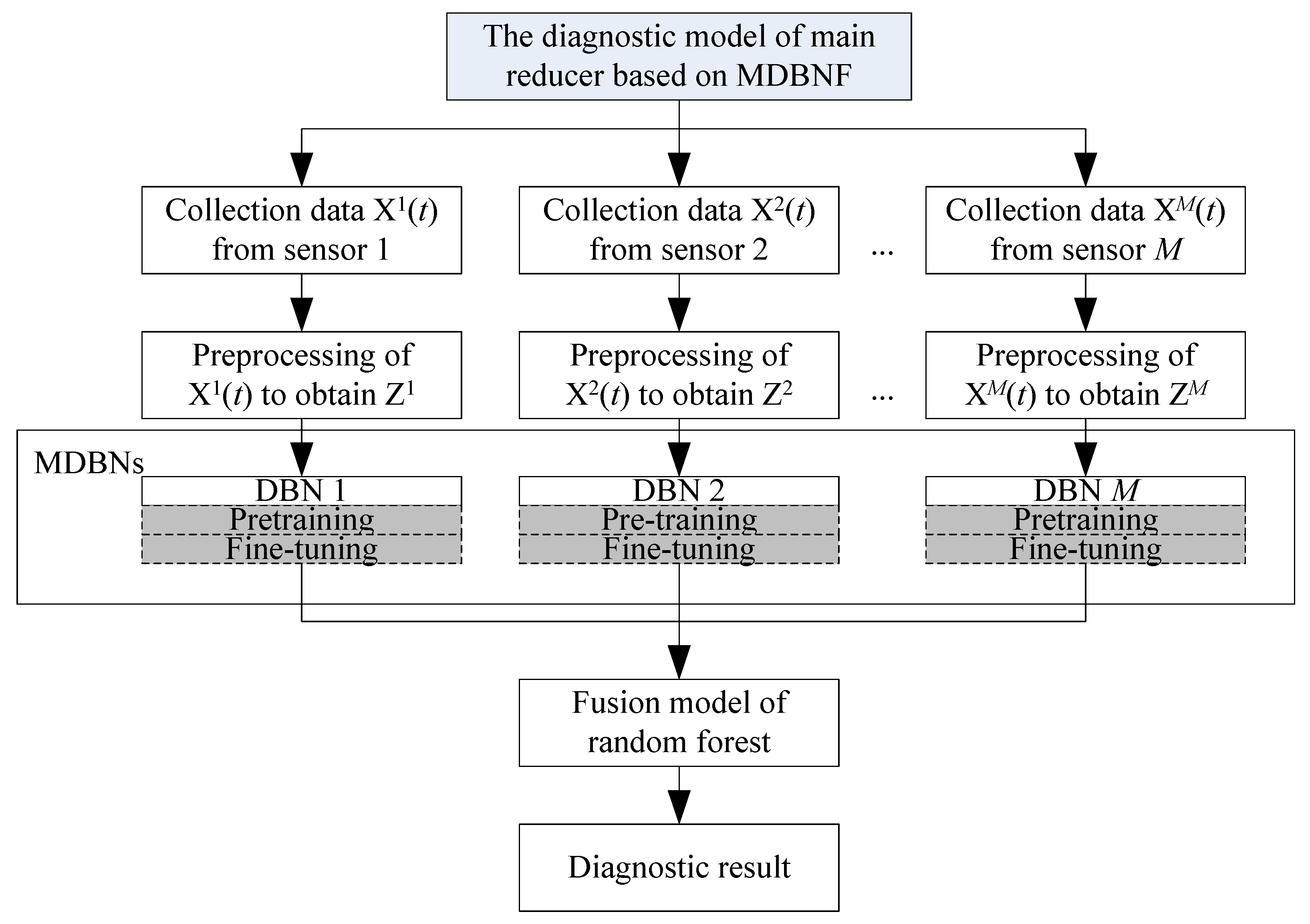
After the MDBNs model is well trained by training sample, it can be used to diagnose fault pattern of main reducer by using vibration measurement of from multiple sensors. The structure of the proposed diagnostic model of MDBNF for main reducer is shown as Figure 4.

The procedure of the proposed diagnostic model of MDBNF for main reducer is described as follows:

Step 1: Collect multichannel vibration signals of main reducer from M sensors expressed as X¹(t), X²(t),…, X^M(t). Define fault patterns for fault diagnosis.

Step 2: Preprocess the collected signals to generate multiple modalities features expressed as ${\mathrm{Z}}^1,{\mathrm{Z}}^2,\dots ,{\mathrm{Z}}^M$ uusing several statistical parameters of time domain, frequency domain and time-frequency domain.

Step 3: Construct the model of MDBNs consisting of multiple DBN structures to implement deep learning of multichannel data, and generate deep representative features expressed as Equation (8).

Step 4: Use fusion model based on the random forest method to fuse deep representative features of MDBNs, and obtain the output vector expressed as Equation (10).

Step 5: With the output of fusion model, the final diagnostic decision is making by using Equation (11).

4. Experiment and Discussion

4.1. Experiment Setup

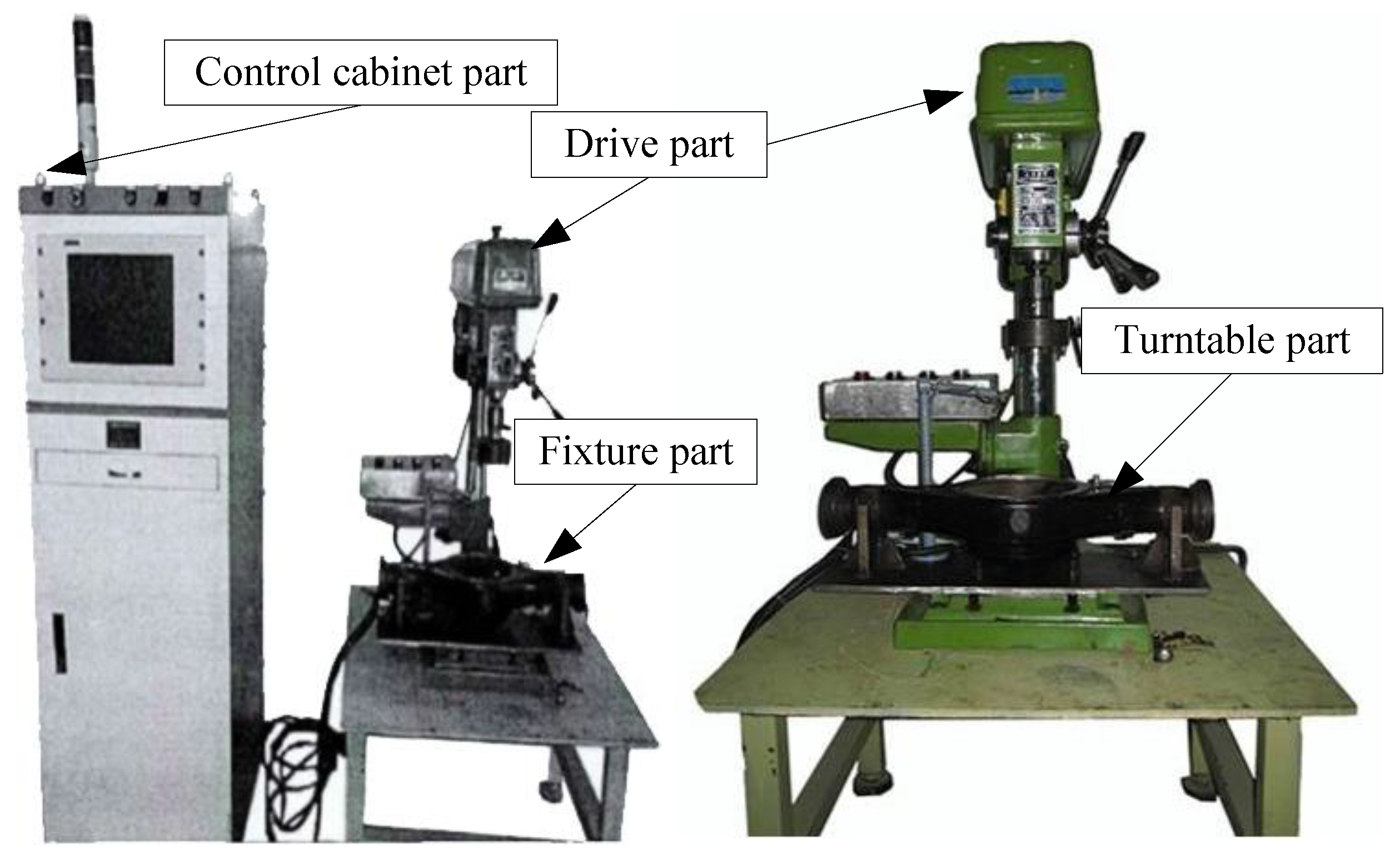
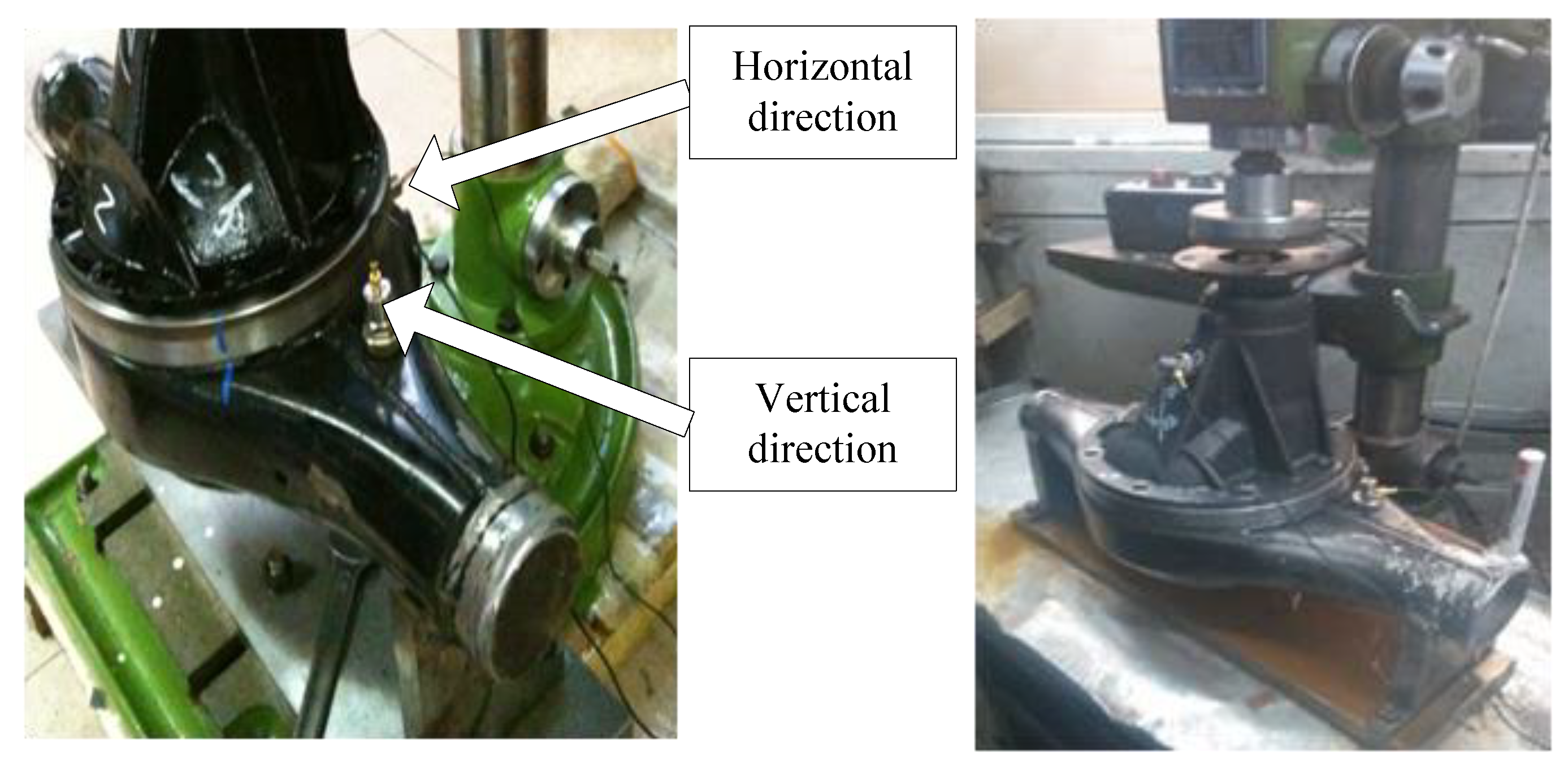
The experiments are carried out on a main reducer fault diagnosis test rig which consists of a control cabinet part used to control the rotating speed and rotating time, a drive part used to start the driving motor and a fixture part used to simulate the running states of main reducer under certain rotating speed. The main reducer test rig is shown in Figure 5. In order to implement reliable condition monitoring of the main reducer to collect multichannel data for fault diagnosis, we install two sensors on the tested main reducer in horizontal direction and vertical direction as shown in Figure 6.

The common faults of the main reducer occur in the pair of gears, including gear error, gear burr, gear hard point, misalignment, gear tooth broken and gear crack, as listed in

Table 1. Condition pattern description.

Fault Pattern	Condition Patterns
C1	Normal status
C2	Gear error
C3	Gear burr
C4	Gear hard point
C5	Misalignment
C6	Gear tooth broken
C7	Gear crack

. Seven condition patterns were simulated at the rotating speed of 1200 rps (revolutions per second) with the sampling frequency of 12 kHz. They contained six fault patterns and the normal condition. We ensured that the sampling frequency is higher than the gear meshing frequency so that effective information of fault can be reserved during sampling.

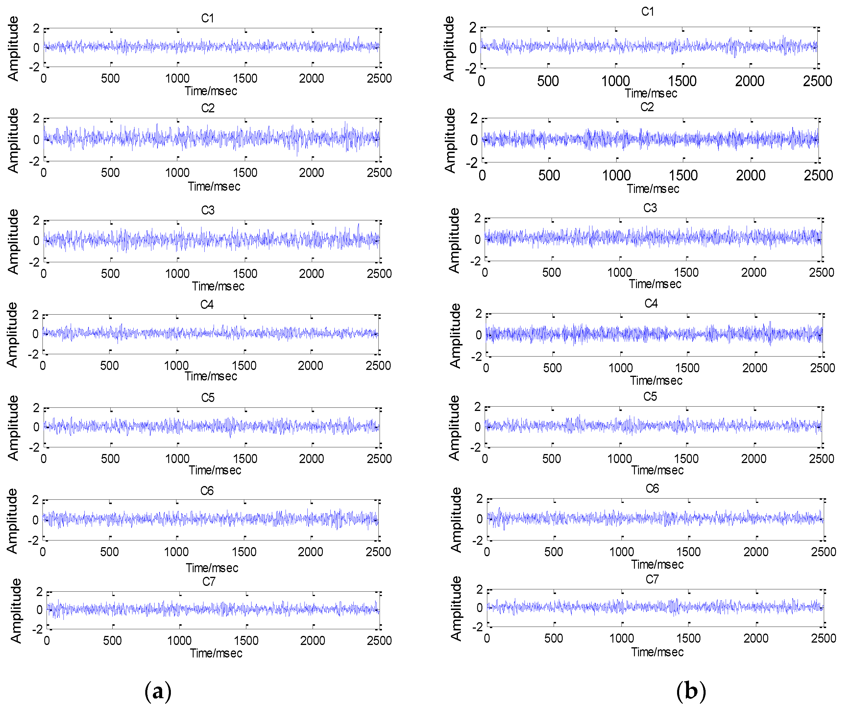
For each condition pattern, we repeated10 tests to collect enough data to represent the pattern. In each test, 20 signals with the duration of 0.2 s were collected. In this way, for each sensor, 1400 vibration signals corresponding to seven condition patterns were acquired in which 1050 signals were used as the training set to train MDBNs model and 350 signals were used as the testing set to test the performance of the model. The collected multichannel vibration signals are expressed as $X^1\left(t\right)=\left[x_1^1\left(t\right),x_2^1\left(t\right),\dots ,x_{1400}^1\left(t\right)\right]$ and $X^2\left(t\right)=\left[x_1^2\left(t\right),x_2^2\left(t\right),\dots ,x_{1400}^2\left(t\right)\right]$. Each experiment was executed for 50 trials.

For each condition pattern, vibration signals collected from two sensors are shown in Figure 7. The simulations of the experiments were implemented in Matlab 7.0 on the computer with CPU of 3.4 GHz and RAM of 4 GB.

4.2. Data Preprocessing

In the preprocessing procedure of raw vibration signals to extract condition parameters, the maximum decomposition level of WPT is 6, and it employs Daubechies wavelet of order 4 (db4) as mother wavelet of WPT. Then, 2⁶ coefficients are obtained by using WPT and the energy of each coefficient is combined to form a set of condition parameters. In this way, multiple modalities features for the vibration signal collected from each sensor with the dimension of 80 are extracted and stored in a matrix of 1400 rows (number of samples) and 80 columns (number of features).

In order to implement deep learning of multiple modalities features extracted from vibration signal of two sensors, two feature sets of 1050 training samples corresponding to seven condition patterns are expressed as ${\mathrm{Z}}^1=\left[{\mathrm{Z}}_1^1,{\mathrm{Z}}_2^1,\dots ,{\mathrm{Z}}_{1050}^1\right]$ and ${\mathrm{Z}}^2=\left[{\mathrm{Z}}_1^2,{\mathrm{Z}}_2^2,\dots ,{\mathrm{Z}}_{1050}^2\right]$, in which ${\mathrm{Z}}_i^1$ and ${\mathrm{Z}}_i^2$ are composed of 80 features extracted from the ith vibration signal, and ${\mathrm{Z}}^1$ and ${\mathrm{Z}}^2$ are used to construct the MDBNs model with two DBNs.

4.3. Model Design

The model of DBN was developed using the principles described in Section 2.1. For vibration signals collected from two sensors, we developed a deep learning model of MDBNs containing two DBNs named DBN1 and DBN2. The number of hidden layers of DBN1 and DBN2 relevant to learning performance and computation burden was set to 2. The number of the hidden neurons for the first hidden layer was set to 50, and the number of hidden neurons for the second hidden layer was set to 30.

In order to train each DBN of MDBNs, the number of pretraining epoch was set to 100, and the number of fine-tuning epochs was set to 200. The dimension of the output vector of MDBNs was 30, which means that the dimension of input for the fusion model was 30. In order to construct the fusion model based on random forest, the number of decision trees was set to 10.

4.4. Experimental Results and Discussions

4.4.1. Results of the Proposed Model of MDBNF

The well-trained diagnostic model of MDBNF was used for main reducer fault diagnosis. By using a testing of 350 samples collected from each sensor corresponding to seven condition patterns, 342 samples were correctly classified, which means that the classification accuracy of the proposed diagnostic model is 97.72%. Additionally, the classification accuracy for different fault patterns is shown in

Table 2. Classification accuracy for different fault patterns.

Fault Patterns	Diagnostic Result							Accuracy
	C1	C2	C3	C4	C5	C6	C7
C1	50	0	0	0	0	0	0	100%
C2	0	49	0	1	0	0	0	98%
C3	0	0	49	0	0	1	0	98%
C4	0	1	0	48	0	0	1	96%
C5	0	0	1	0	49	0	0	98%
C6	0	0	0	0	1	49	0	98%
C7	0	1	0	0	0	1	48	96%

. Table 2 indicates that the proposed diagnostic model is available for effectively diagnosing seven fault patterns of the main reducer, and is completely suitable for diagnosing normal status with the classification accuracy of 100%.

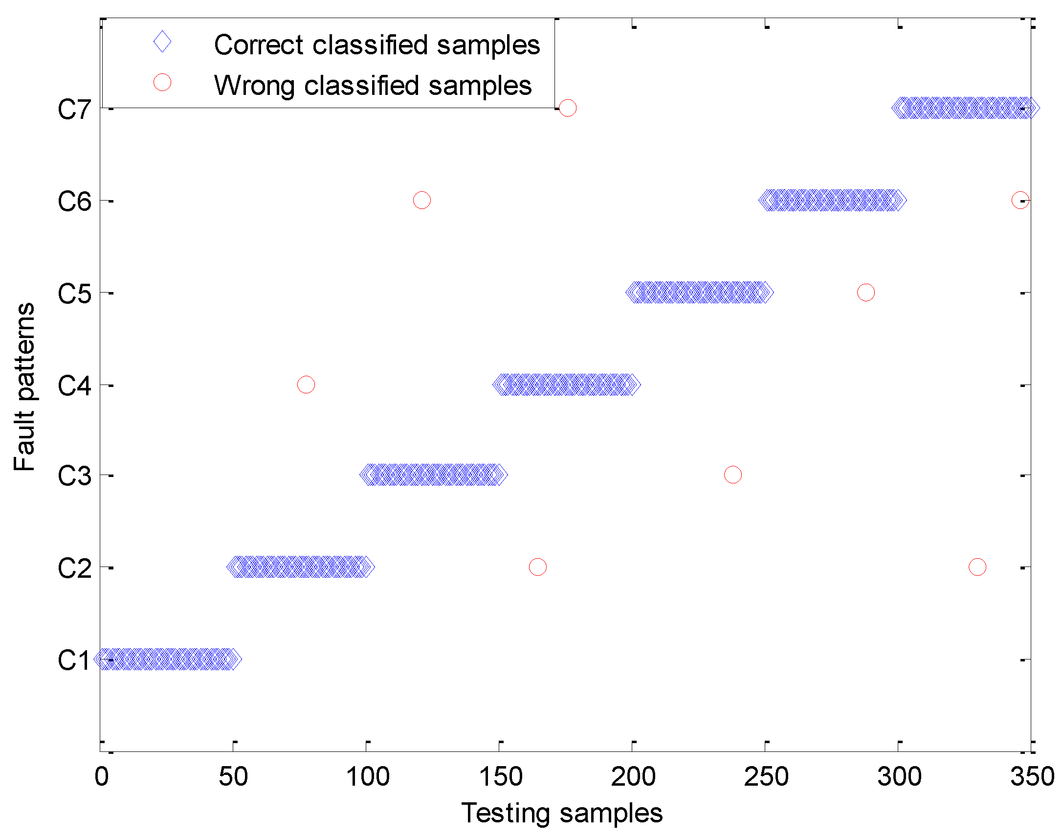
A set of detailed diagnostic result of MDBNF in one trial is shown in Figure 8 for intuitive presentation. The detailed diagnostic result in Figure 8 shows that the vast majority of samples in the testing set can be correctly classified by the proposed model of MDBNF.

The superiority of the proposed diagnostic model is to employ vibration signals collected from multiple sensors so as to significantly enhance the reliability and sensitivity between captured symptom and fault patterns. With the multichannel data, a fusion model based on random forest was used to fuse the multiple modalities features extracted from these multichannel data.

4.4.2. Principal Component Analysis of the Deep Representative Features

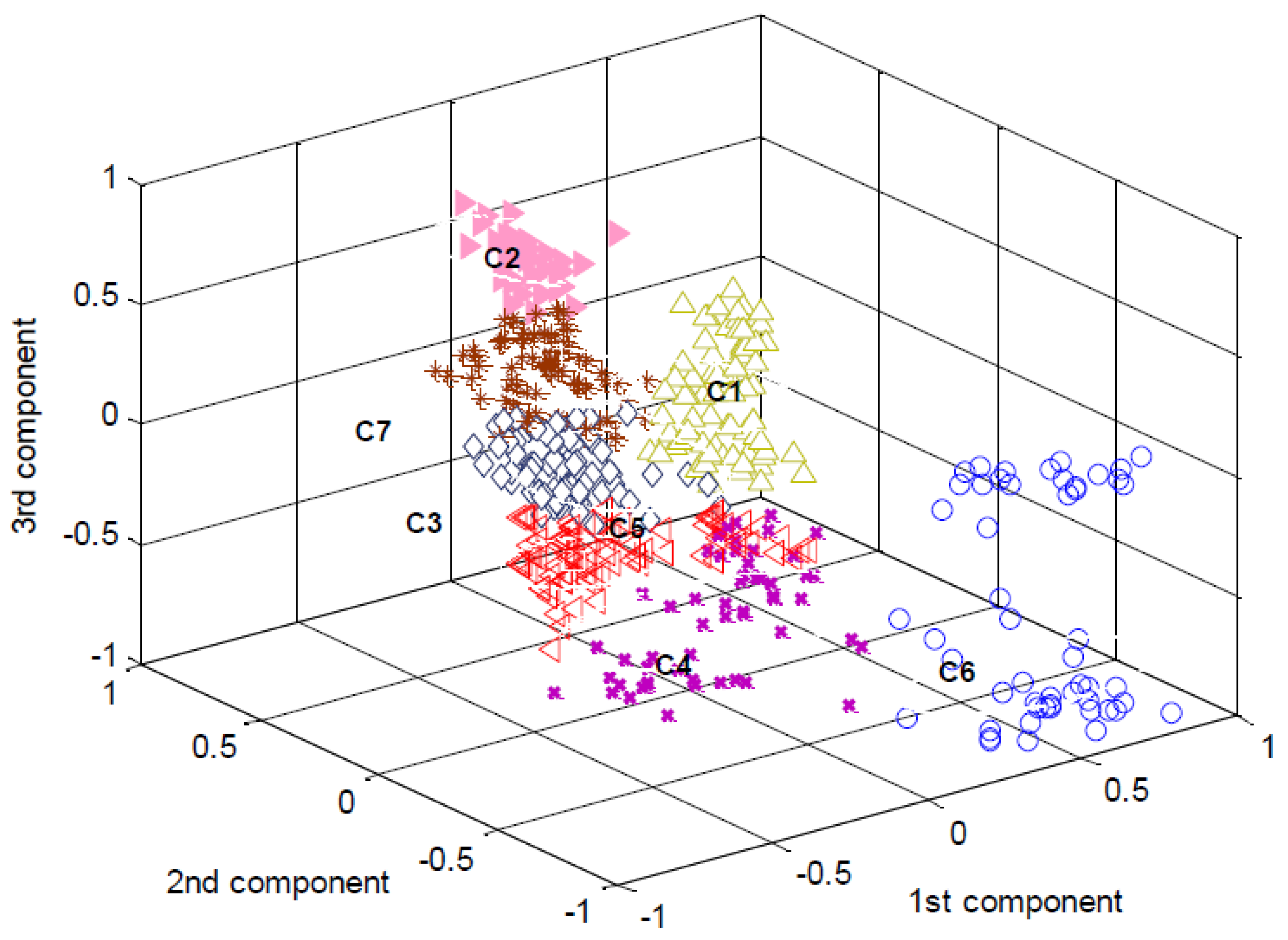
To verify the ability of MDBNs for deep learning of fault-sensitive features, we utilized principal component analysis (PCA) to visualize the deep representative features obtained from MDBNs. The dimension of output vector of MDBNs is 30.PCA was carried out on 30 features of each sample, and the top three principal components of the feature vector of testing setare shown in Figure 9.

As shown in Figure 9, most points corresponding to the same fault pattern are clustered together, and points corresponding to different fault patterns are mostly separated to some extent. Considering that the section of features only have the top three principal components of feature vector with the aim of visualization, so that some useful information have been neglected. Although the points obtained by PCA can’t be used to directly achieve superior classification accuracy of several fault patterns, the entire deep representative feature obtained from MDBNs is fault-sensitive and is quite qualified for classification. The result revealed that the proposed MDBNs could adaptively mine the deep representative characteristics of the main reducer.

4.4.3. Effectiveness of the Fusion Model

In order to validate the effectiveness of the fusion model for multichannel data in the proposed diagnostic model, by using a typical testing sample composed of $x_{268}^{1\prime }\left(t\right)$ and $x_{268}^{2\prime }\left(t\right)$ collected from two sensors, we conducted a comparison experiment which includes three situations: the first situation is to directly use deep representative features $p^1$ of the testing sample $x_{268}^{1\prime }\left(t\right)$ outputted from DBN1 as input of classifier, the second situation is to directly use deep representative features $p^2$ of the testing sample $x_{268}^{2\prime }\left(t\right)$ outputted from DBN2 as input of classifier, the third situation is to use fusion model based on random forest to fuse the output of the entire MDBNs expressed as $\left(p^1,p^2\right)$ to acquire the final diagnostic result by majority voting operation. The output of above three situations and comparison results of classification accuracy testing set are shown in Figure 10.

According to Figure 10a–c, the diagnostic results of directly using deep representative features $p^1$ and $p^2$ of the testing sample $x_{268}^{1\prime }\left(t\right)$ and $x_{268}^{2\prime }\left(t\right)$ are totally incorrect, namely C5 and C3. However, the output of fusion model for $\left(p^1,p^2\right)$ could reflect the actual fault pattern of the testing sample, namely C6. Without fusion of multichannel data, the output of the classifier with input of deep representative features $p^1$ and $p^2$ outputted from DBN1 and DBN2 are inferior to the output of fusion model. The results reveal that the vibratory measurements using a single sensor may result in wrong fault patterns; the proposed diagnostic model with data fusion can lead to correct classification results.

As shown in Figure 10d, without data fusion, classification accuracy of testing set collected from sensor 1 and sensor 2 are 88.35% and 88.73%. The comparison result indicates that the multichannel data fusion of the proposed diagnostic model can effectively improve the relevance between collected vibration signals and fault patterns so as to enhance the diagnostic performance by nearly 8%.

4.4.4. Comparison of Different Diagnostic Models

In order to validate the superiority of the proposed diagnostic model based on MDBNs and data fusion of multichannel data, we implemented a set of experiments of comparing some state-of-the-art methods in the field of fault diagnosis by using the same sample set.

The compared diagnostic models include: (1) the proposed diagnostic model of MDBNF, (2) diagnostic model with MDBNs structure and KNN fusion, (3) diagnostic model with MDBNs structure and support vector classification (SVC) fusion, (4) diagnostic model with deep learning of single sensory data and without data fusion, (5) diagnostic model with shallow learning of representative features of multichannel data, (6) diagnostic model with shallow learning of representative features of single sensory data. Twenty trials are carried out for each model. The average classification accuracies of all comparison diagnostic models in the experiments are shown in

Table 3. Average classification accuracy of different diagnostic models.

No.	Data Type	Learning Level	Diagnostic Models	Accuracy
(1)	Multichannel	Deep learning	MDBNF	97.72%
(2)	Multichannel	Deep learning	MDBNs with KNN fusion	94.63%
(3)	Multichannel	Deep learning	MDBNs with SVC fusion	95.79%
(4)	Single-channel	Deep learning	DBN	88.58%
(5)	Multichannel	Shallow learning	SVM	73.16%
(6)	Single-channel	Shallow learning	SVM	74.37%

.

From Table 3, we can conclude as follows:

(1)

With the same deep learning architecture of MDBNs, average classification accuracies of diagnostic models that use KNN and SVC to fuse deep representative features of multichannel data have reached 94.63% and 95.79%. However, the performances of these two models are still inferior to the proposed model of MDBNF that uses random forest fusion for multichannel data with the accuracy of 97.72%. It indicates that random forest fusion with majority voting strategy is better than simple classification strategy of KNN and SVC.MDBNF can fuse deep features outputted from DBNs with the input of multichannel data to obtain the final result in higher layer.

(2)

Without using multiple sensors to collect vibration signals, the performance of the DBN model with deep learning of single sensory data is 88.58%, which is not ideal and inferior to models with multichannel data fusion. It indicates that sensory data in different channels may contain various failure-sensitive characteristics. Therefore, multichannel data could exhibit more complete characteristic information of the main reducer.

(3)

The classification accuracies of models based on SVM with shallow learning of representative features are the worst, namely 73.16% and 74.37%, no matter which kind of data is selected. It indicates that deep learning architecture indeed extracts more fault-sensitive features of main reducer than shallow learning and could effectively establish non-linear relationships between vibration measurements and fault patterns of main reducer.

(4)

Compared with all the peer models, the performance of the proposed diagnostic model of MDBNF with multichannel data is superior to other models for main reducer fault diagnosis. This phenomenon indicates that multichannel data and deep learning architecture can improve the reliability and accuracy for fault diagnosis.

5. Conclusions

In this paper, a multichannel data fusion method based on a deep belief network and random forest fusion is proposed for fault diagnosis of the main reducer. Collecting vibration signals with a single sensor may encounter limitations in the location and orientation of the sensor installation. To track this issue, multiple channels of data were collected by using multiple sensors to display more complete feature information. Then, we were able to construct the structure of multiple deep belief networks (MDBN) to deeply learn representative features from multichannel data. Finally, an MDBNF model was established to randomly fuse multiple features of MDBN to obtain the final diagnosis result. In order to confirm the effectiveness and efficiency of the proposed diagnostic model, we implemented a set of comparison experiments by using a main reducer fault test rig. The experiment results verify the effectiveness of the proposed method, which achieves the best testing accuracy among all the comparative methods in the experiments.

The method proposed in this paper is effective, but there are still some limitations in the number of sensors, sensor types and operating conditions. Our future work will focus on testing the diagnostic model of MDBNF based on a multichannel data fusion method on more sensor quantity, sensor types and operation conditions. Furthermore, with the purpose of offering reasonable maintenance proposal, it is meaningful to investigate more effective approaches that can correctly diagnose the severity of several fault patterns after fault recognition.