Classification of Guillain–Barré Syndrome Subtypes Using Sampling Techniques with Binary Approach

Abstract

Guillain–Barré Syndrome (GBS) is an unusual disorder where the body’s immune system affects the peripheral nervous system. GBS has four main subtypes, whose treatments vary among them. Severe cases of GBS can be fatal. This work aimed to investigate whether balancing an original GBS dataset improves the predictive models created in a previous study. purpleBalancing a dataset is to pursue symmetry in the number of instances of each of the classes.The dataset includes 129 records of Mexican patients diagnosed with some subtype of GBS. We created 10 binary datasets from the original dataset. Then, we balanced these datasets using four different methods to undersample the majority class and one method to oversample the minority class. Finally, we used three classifiers with different approaches to creating predictive models. The results show that balancing the original dataset improves the previous predictive models. The goal of the predictive models is to identify the GBS subtypes applying Machine Learning algorithms. It is expected that specialists may use the model to have a complementary diagnostic using a reduced set of relevant features. Early identification of the subtype will allow starting with the appropriate treatment for patient recovery. This is a contribution to exploring the performance of balancing techniques with real data.

1. Introduction

1.1. Guillain–Barré Syndrome

Guillain–Barré Syndrome (GBS) was initially detected in 1916 by Guillain, Barré and Strohl. It is a rare acute paralytic polyneuropathy with four principal several clinical variants. It is an autoimmune disorder of the peripheral nervous system [1]. GBS characterizes by a fast development normally from a few days up to four weeks with an incidence closely to one to two in 100,000 people. It occurs in adults and children. GBS can damage the nerves controlling movements, pain, temperature, and touch sensations [2]. In critical cases, GBS may lead to respiratory failure and can also be mortal. The progression of GBS can be described in three phases:

1

Initial phase: evolution of symptoms lasting days to up to four weeks

2

Plateau phase: lasting weeks to months

3

Recovery phase: remyelination, lasting weeks to months. Critical patients can take a minimum of two years or more. Full recovery is not achieved in some cases.

The exact cause is unknown but frequently is associated with a respiratory or gastrointestinal infection. Cytomegalovirus and Zika are associated with GBS [3].

The GBS subtypes are mainly [4]:

• Acute Inflammatory Demyelinating Polyneuropathy (AIDP)
• Acute Motor Axonal Neuropathy (AMAN)
• Acute Motor Sensory Axonal Neuropathy (AMSAN)
• Miller–Fisher Syndrome (MF)

Table 1. Features of GBS subtypes [5].

Type	Symptoms	Pathology
AIDP	Most common variant (85% of cases). Primarily motor inflammatory demyelination ± secondary axonal damage. Maximum of four weeks of progression.	Macrophages invade intact myelin sheaths and denude the axons.
AMAN	Motor only with early and severe respiratory involvement. Primary axonal degeneration. Often affects children, young adults. Up to 75% positive Campylobacter jejuni serology. Often positive for anti-GM1, anti-GD1a antibodies.	Macrophages invade the nodes of Ranvier where they insert between the axon and the surrounding Schwann-cell axolemma, leaving the myelin sheath intact.
AMSAN	Motor and sensory affection with critical course of respiratory and bulbar involvement. Primary axonal degeneration with poorer prognosis.	Similar to AMAN but also involving vetral and dorsal roots.
MF	Ophthalmoplegia, sensory ataxia, areflexia. 5% of all cases. 96% positive for anti-GQ1b antibodies.	Abnormality in sensory conduction, although the underlying pathology is not clear.

[5] describes the characteristics of each of the GBS subtypes.

The first approach in the diagnosis of GBS is based upon the clinical features since it is a non-invasive method. Nevertheless, diagnostic mechanisms such as cerebrospinal fluid (CSF) analysis and electrodiagnostic studies are useful to determine the specific subtype that the patient is suffering [6]. These methods have several disavantages since they are invasive and costly. In this exploratory study, we used different sampling methods, to balance the GBS multiclass dataset. We aimed to create different predictive models using real data to identify four main GBS subtypes that a patient suffers, applying Machine Learning algorithms. It is expected that specialists may use the model to have a complementary diagnostic using a reduced set of relevant features. Early diagnosis of the GBS subtype is essential due to the rapid progress of this disorder. The treatments vary according to the subtype contracted. Sequelae and economic costs can be high unless proper treatment is started immediately.

1.2. Imbalanced Data Classification

A dataset is imbalanced when one of its classes has fewer instances (minority class) regarding the other class (majority class) [7]. purple One instance is a row in a dataset. For this study, there are 129 instances that belong to patients diagnosed with some type of GBS. Classes are the way the data is grouped in a dataset. For example, in this work, there are four classes in the original dataset. Each class represents a subtype of GBS. Standard classifiers are designed to work with balanced datasets. When a dataset is imbalanced, the classifiers take the majority class for decision making, ignoring the minority class. It affects the performance of the classifiers because, in real-life cases, it generally needs to find the classification of the minority class [8]. For example, in cases of cancer diagnosis, there are more healthy patients than those diagnosed with the disease. If we apply a classifier to imbalanced data to identify cancer patients, the classifier biases the result to healthy patients (majority class) ignoring cancer patients (minority class). The accuracy will be high; however, it is more important to identify cancer patients than healthy patients.

There are two types of imbalance data. Binary imbalance occurs when in a dataset is integrated with two classes, one of them has fewer instances (minority class) than the other class (majority class). On the other hand, the multiclass imbalance is present when the dataset has more than two classes and the instances that form them are unequal with respect to the others [9]. There are three main methods used in the literature to handle imbalanced data:

∗

Algorithm Level: It makes a modification to the algorithm, generally adds more weight to the minority class. This method requires a deep knowledge of the operation of the algorithm to be modified. Each algorithm must be adapted to the dataset to be used.

∗

Data Level: It consists of balancing the training set by matching the majority class with the minority class. This method is known as preprocessing since the modification of the data is done before the application of the classification algorithm. Standard classifiers are designed to work with a balanced dataset. The advantages of this method are that they are easy to configure, and they can be used with any classification algorithm. There are three sampling methods:

☉

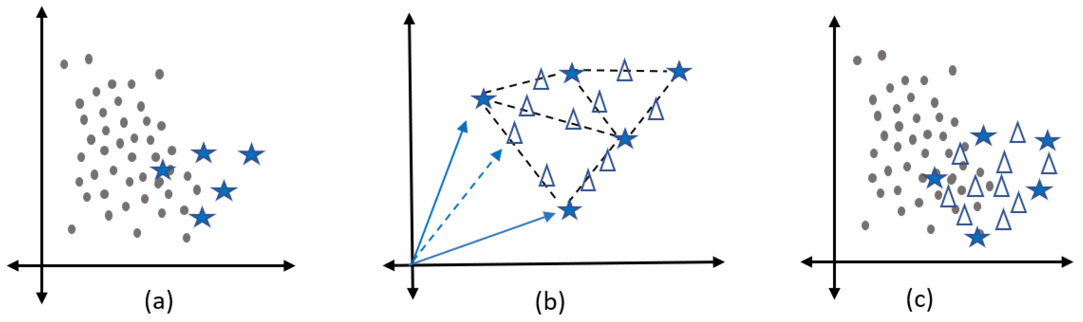
Undersampling: It consists of eliminating instances of the majority class until matching the number of instances with the minority class. There are other undersampling variants that eliminate instances in a directed manner such as noise or instances that are in the border of the decision area.

☉

Oversampling: This method adds instances to the minority class until the majority class is balanced with the minority class. There are different variants for oversampling. For example, Random Oversampling (ROS), makes a copy of existing instances and adds a copy of them randomly. SMOTE is one of the most successful methods for oversampling. This adds instances in synthetic form to the minority class. There are also variants of SMOTE which have demonstrated great precision.

☉

Hybrid: It is the combination of the different Oversampling and Undersampling methods.

∗

Cost-sensitive: Combines the methods of Data level and Algorithm Level. It is considered the costs associated with misclassifying.

Preprocessing methods have shown that balancing the training set by oversampling and undersampling of classes improves significantly the classifiers results. This regarding imbalanced data [10,11,12].

The goal of this research was to identify the best algorithm to balance Guillain–Barré Syndrome (GBS) dataset by applying different data balancing techniques at the data level, oversampling the minority class and undersampling the majority class. purpleIn the specialized literature, there are no studies to classify the subtypes of GBS using Machine Learning algorithms. In previous studies, [13,14], predictive models were created to classify the four main GBS subtypes using different classifiers. These models were created using an imbalanced dataset obtained an accuracy of 90%. In this experimental study, the data was preprocessed using different balancing techniques to balance the original dataset. With the objective that the classifiers use balanced data and know if it is possible to overcome the previously created models. The results show that balancing the data helps in the performance of predictive models. In some cases improved 90% accuracy.

In this study, purplewe try to make symmetrical the number of instances of each subtype by applying four different undersampling algorithms (Random Undersampling -RUS-, Tomek Link -TM-, One Side Selection -OSS- and Neighborhood Cleaning Rule -NCR-). Then, we compared these results with those found by Synthetic Minority Oversampling Technique (SMOTE) using different percentages of oversampling. We binarized the multiclass dataset with two different techniques: One versus All (OVA) and One versus One (OVO). We used three classifiers with different approaches: Decision tree (C4.5), Support Vector Machines (SVM) and JRip. purple Decision tree and JRip create predictive models understandable by humans and this is an advantage, especially in this case, models obtained may be useful for physicians to diagnose GBS subtypes. Moreover, C4.5, JRip, and SVM stand out their excellent results in classification tasks.

The goal was to investigate whether data balancing techniques allow to create a predictive model with a statistically significant difference with respect to a predictive model with imbalanced data.

This article is organized as follows. In Section 2, we show a literature review. Section 3, we present a description of the dataset, machine learning algorithms and the performance measure used in the study. Section 4 describes the experimental procedure. In Section 5, we show and discuss the experimental results. Finally, in Section 6, we summarize results, provide conclusions, and suggest future work.

2. Related Work

In real life, the imbalance data is frequent in cases of medical diagnosis or in the identification of variants of diseases. The main problem occurs because of existing more cases of healthy patients than patients with any disease. For this type of challenge, researchers have applied data preprocessing techniques which consist of oversampling the minority class or undersampling the majority class. These techniques have shown that balancing datasets significantly improve the performance of classifiers.

In [15], Han and coworkers proposed Distribution-Sensitive (DS). This is an oversampling algorithm for Medical Diagnosis for imbalanced data. DS analyzes the position of the minority class instances and carefully classifies them into noise samples, unstable samples, limit samples, and stable samples. Each of these samples is processed differently by the algorithm. The objective is to choose the most suitable sample to synthesize new samples. Authors apply sample synthesis methods according to the closeness among surrounding samples, and thus guarantee that the newly synthesized samples and the original minority samples share characteristics. The results showed that the accuracy of the classification algorithm is improved.

Bach et al., in 2016 [16], analyzed a dataset of 729 patients. In total, 92.6% belonged to healthy cases and 7% of cases suffered from Osteoporosis. For this imbalanced data, the authors applied oversampling and undersampling methods to detect patients with Osteoporosis. To oversample the dataset, they applied SMOTE. To undersample, they used two different methods, Random Undersampling (RU) and Edited Nearest Neighbours (ENN). Bach found that SMOTE at 300% combined with ENN gave the best results.

Kalwa et al. [17] a Smartphone Application was used to diagnose melanoma which is a type of skin cancer, considered the most deadly and difficult to treat in advanced stages. The application analyzes images and compares them with 200 images of a public dataset. This research uses SMOTE to oversampled cases of melanoma patients. The results were compared without using any preprocessing technique, resulting in SMOTE obtaining better performance regarding the data not oversampled.

In [18], Le et al. propose a framework for self-care problems detection of children with physical and motor disabilities. This research uses SMOTE to improve the prediction for the SCADI (Self-Care Activities Dataset) dataset. The results show that extreme gradient boosting using SMOTE outperforms Artificial Neural Network, Support Vector Machine and Random Forest (RF). The accuracy of their framework reaches 85.4%.

Fazal proposes a Hybrid Prediction Model (HPM) [19]. This study analyzes a dataset to improve early diagnosis of Type 2 Diabetes and Hypertension. HPM consists of Density-based Spatial Clustering of Applications with noise-based outlier detection, SMOTE, and RF. The authors successfully predict diabetes and hypertension using three benchmark datasets.

Elreedy et al. [20], conducted an experimental study to explore SMOTE performance factors, analyzing the relationship between the number of records created and the dataset dimension. They also analyzed the performance of some classifiers and the effects of applying SMOTE. Finally, they included in the study some variants of SMOTE such as Bordeline_SMOTE1, Borderline_SMOTE2 and ADASYN and their performance. For this work, they used five public datasets taken from UCI. As a result, they found that SMOTE improves the performance of the classifiers, however, this varies from one type of classifier to another. They found that the more examples of the minority class exist, the greater the accuracy. This is because the K-nearest neighbor patterns become closer to each other. They concluded that SMOTE can be used in classification problems for small datasets since increasing the size of the data improves the classification performance.

In [21], Devi and coworkers presented a modification of the Tomek Link undersampling algorithm, based on the fact that, in addition to class imbalance, there are other factors such as the existence of redundant borderline records and outliers in the data space that critically reduce the performance of classifiers. They used 10 public UCI datasets and four single classifiers for their experiments. The proposed algorithm facilitates the removal of redundant boundary records rather than simple boundary ones, with the aim of creating a sparse majority region near the decision boundary. This may help to convergence towards a balanced class distribution. This undersampling method achieves less loss of information and better performance.

Bach et al. [22], compared four different undersampling methods to balance data: Edited Nearest Neighbor, Neighborhood Cleaning Rule, Tomek Link, and Random Undersampling, against his proposed algorithm, called KNN_Order. This algorithm removes records from high-density areas to minimize loss of information. They proved the performance of this algorithm using 18 public datasets.

In addition to class imbalance and noise, the superposition of instances of different classes affects the performance of classifiers. In [23], they proposed to remove potentially overlapped data points to tackle binary class imbalance, using Neighborhood search with different criteria. This method identifies and eliminates instances of the majority class. They use 66 synthetic datasets and 24 public datasets of UCI and Keel repository in their experiments. These methods were compared with other balancing methods, achieving competitive performance over traditional methods.

In [24] Kovacs et al., they performed a detailed comparison of 85 variants of oversampling techniques for the minority class. They used 104 imbalanced datasets as well as four classifiers for their experiments. They found that oversampling leads to better results in classification on imbalanced datasets. Regarding SMOTE variants, polynom-fit-SMOTE, ProWSyn, and SMOTE-IPF gave the best results.

In [25], introduced Farthest SMOTE (FSMOTE), a modification of SMOTE. This approach increases the decision area, considering minority samples closer to the boundary. They compare different oversampling methods: SMOTE, ADASYN, borderline SMOTE, and safe-level SMOTE. For experiments, they used seven datasets and two classifiers: Naive Bayes and SVM. Results showed that FSMOTE improves the existing techniques.

Debashree and coworkers [26] proposed a modification of the Tomek-Link undersampling method. They present a solution to class imbalance and classes overlapping, as these two problems affect the performance of standard classifiers. The objective of their research was overlapping region detection, cleaning up of overlapping region, undersampling of the majority records, and an effective data-preprocessing framework. The proposed model increases the performance of the minority class while maintaining an intact majority class performance.

On the other hand, there are several studies employing bioinformatics thechniques, such as microarray tests [27]. However, the most significant disadvantage of microarrays is the high cost of a single experiment.

The data balancing through sampling methods can be applied to any imbalanced dataset, regardless of the subject. In finance, the classification can be improved, for example:

In [28] SMOTE was applied to create Financial risk models. These models serve companies to prevent threats from the external economic environment or bad financial decisions. In this study, the authors used 2628 Chinese companies listed on the stock exchange. The imbalance occurs because there are more companies with healthy finances (2190 belonging to the majority class) than companies with financial risk (438 belonging to the minority class). They performed three types of experiments: In the first experiment, they used the imbalanced data and applied Adaboost and Support Vector Machine (SVM). In the second experiment, they applied data balancing with SMOTE and subsequently applied Adaboost with SVM. For the third experiment, they executed Adaboost with SVM, however, SMOTE worked at the same time that the classifiers. The results show that balancing the data improved the models with the imbalanced data. For balanced models, the third model improved a significant difference with the second model.

Online banking operations using credit cards have been increasing every day; with this growth, credit card frauds are also more common. In [29] Sisodia et al. made models using different sampling methods to identify credit card fraud detection. They applied five different oversampling methods (SMOTE, SMOTE-ENN, SMOTE-TL, Safe-SMOTE, and ROS). On the other hand, they used four different undersampling methods (RUS, CNN, CNN-TL, and TL) and three different datasets DS1 with 10,000 transactions (38 fraud and 9961 normal transactions), DS2 with 15,000 transactions (50 fraud and 14,950 normal transactions) and DS3 with 20,000 transactions (53 fraud and 19,947 normal transactions). They applied four different classifiers (SVM, C4.5, Adaboost, and Bagging) with four different performance metrics (Area under ROC Curve, Sensitivity, Specificity, and G-Mean). The results showed that the best classifiers were Bagging and SVM. SMOTE-ENN obtained the best performance compared to the other oversampling methods. For the undersampling methods, TL obtained the best performance.

Phishing is a technique used by cybercriminals to deceive and obtain personal information such as passwords, credit card data, and bank account numbers. This is achieved through fraudulent emails. A large amount of mail sent and received can help build models with Machine Learning algorithms that help predict future cyber-attacks. However, most of the emails that reach us in the inbox are true compared to phishing emails. This results in an imbalance of data. In [30], they used SMOTE to balance a dataset with 812 instances obtained from the UCI Machine Learning Repository. The dataset is divided into three classes (phishy, suspicious and legitimate). Three algorithms were used to create the models (Support Vector Machine, Random Forests, and XGBoost). The results show that the imbalanced data have poor performance. The data that were balanced using SMOTE achieved a better performance.

3. Materials and Methods

3.1. Dataset

The dataset used in this work are records of 129 cases of patients diagnosed with Guillain–Barré Syndrome (GBS). They received treatment for one of the four subtypes of GBS: AIDP, AMAN, AMSAN and MF. The data were collected at the Instituto Nacional de Neurología y Neurocirugía.

Table 2. Dataset characteristics.

Dataset	Number of	Number of	Number of	Class 1	Class 2	Class 3	Class 4
Name	Classes	Instances	Attributes	AIDP	AMAN	AMSAN	MF
GBS	4	129	16	20	37	59	13

shows the characteristics of the dataset.

Table 3. Variables used in this work.

Feature Label	Feature Name	Feature Type
v22	Symmetry (in weakness)	Clinical
v29	Extraocular muscles involvement	✓
v30	Ptosis	✓
v31	Cerebellar involvement	✓
v63	Amplitude of left median motor nerve	Nerve conduction test
v106	Area under the curve of left ulnar motor nerve	✓
v120	Area under the curve of right ulnar motor nerve	✓
v130	Amplitude of left tibial motor nerve	✓
v141	Amplitude of right tibial motor nerve	✓
v161	Area under the curve of right peroneal motor nerve	✓
v172	Amplitude of left median sensory nerve	✓
v177	Amplitude of right median sensory nerve	✓
v178	Area under the curve of right median sensory nerve	✓
v186	Latency of right ulnar sensory nerve	✓
v187	Amplitude of right ulnar sensory nerve	✓
v198	Area under the curve of right sural sensory nerve	✓

shows the 16 relevant features selected in a previous study [31]. These attributes were selected from the original dataset with 365 features. The features V22, V29, V30, and V31 are integer values; the remaining ones are decimal.

3.2. Imbalance Ratio

In binary classification, it is common to find real-life cases where highly imbalanced data are present. An example is credit card fraud detection, where more cases of operations carried out correctly than fraudulent operations are usually found [32]. However, in cases where the number of records of one class is similar to another one it is not clear to determine when a dataset is imbalanced. For example, in [33] the researchers classified three types of different pediatric brain tumors with a dataset of 90 patients divided into three classes: 38, 42, and 10. In cases like this, there is no consensus among experts in the field if there is an imbalance of data between classes.

Imbalance ratio (IR) is the widely accepted measure to determine imbalance data. In Equation (1), IR is the ratio of the number of records of the majority class between the number of records of minority class [34]. A dataset can be considered imbalanced if IR > 1.5 [35].

$$IR=\frac{Majorityclass}{Minorityclass}$$

(1)

For example, we have a binary imbalance dataset composed for $D=C_1,C_2$ where $C_1=46$ (majority class) and $C_2=22$ (minority class). For this dataset, $IR=2.09$, according to Equation (2).

$$IR=\frac{46}{22}$$

(2)

3.3. Machine Learning Algorithms

In this study, we include four methods of undersampling with different approaches. These methods have demonstrated their success to improve the performance of classifiers by eliminating instances of the majority class [36]. We applied these methods to investigate if eliminating random instances of the majority class affects the performance of classifiers. On the other hand, it is proven that not only the imbalance between classes affects the performance of classifiers, but also factors such as noise affect the result [37]. For this reason, we apply three different undersampling methods for noise elimination. We also apply SMOTE, the most commonly used method for oversampling the minority class with synthetic data, using six different synthetic oversampling percentages. This method has demonstrated its success with imbalanced datasets [38]. We used three classifiers from different family, we wanted to investigate which of them gets the best performance compared to those reported in previous studies using the imbalanced dataset.

3.3.1. Random Undersampling (RUS)

RUS is a non-heuristic method of randomly reducing data. RUS takes the majority class and randomly removed the requested instances according to the percentage required in the algorithm. This with the objective of equalizing the majority class with the minority class until reaching the desired balance between the two classes [39]. One of the advantages of this method is that it decreases the run time [40].

3.3.2. Tomek Link (TML)

It is one of the most used data undersampling techniques [41]. TML is based on the Condensed Nearest Neighbor algorithm. TML is also known as a data cleaning method since it eliminates noise from the majority or minority class. On the other hand, TML does not perform data balancing between classes, however, it looks for Tomek examples and only deletes examples of the majority class for each Tomek Link found. The algorithm works as follows: A couple of records $m_i$ and $m_j$ is name the Tomek Link if they are from different classes and are closer neighbors one another. Namely, there is no record $m_l$, in such a way $d(m_i;m_l)<d(m_i;m_j)$ or $d(m_j;m_l)<d(m_i;m_j)$, where $d(m_i;m_l)$ is the distance between $m_i$ and $m_l$. Two records building up a Tomek Link indicates that one of them is noise or both are at the limit [42].

3.3.3. One Side Selection (OSS)

OSS is the combination of two different undersampling methods that carefully remove records of the majority class. First, OSS applies Condensed nearest-neighbor US-CNN, which removes records of the majority class being far from the decision area boundary (redundant examples). Subsequently, OSS uses TML to remove records of the majority class that are noisy examples and also instances that are at the border of the decision area (unsafe examples). Instances of the majority class that were not eliminated are used for learning (safe examples) [43]. Algorithm 1 shows OSS steps.

Algorithm 1: One Side Selection (OSS).

The objective of OSS is to balance the training set keeping only the most significant records of the majority class without eliminating instances of the minority class [44].

3.3.4. Neighborhood Cleaning Rule (NCR)

NCR is a modification of the Edited Nearest Neighbor Rule (ENN) [45]. NCR improves the data cleanliness of the majority class for imbalanced data binary. NCR stands out among other undersampling methods because it considers the quality of the deleted data. It is focused only on data cleansing rather than on the balance of classes of the training set [46].

NCR works as follows: for each record, there is a $N_1$ sample in the training set. Then, find the three closest neighbors of each sample. When $N_1$ belongs to the majority class and the classification outcome is the opposite of the original class at $N_1$, then $N_1$ is removed. When $N_1$ belongs to a minority class and the neighbors belong to the majority class, then the nearest neighbor is removed. [47]. Algorithm 2 shows NCR steps.

Algorithm 2: Neighborhood Cleaning Rule (NCR).

NCR eliminate outlier in the majority class of imbalanced datasets [48].

3.3.5. Synthetic Minority Oversampling Technique (SMOTE)

In [49], SMOTE was introduced, one of the most successful and commonly used oversampling methods in cases of binary class imbalance problems. This technique oversamples the minority class by creating synthetic or artificial data based on the similarities of the feature space between existing minority examples. SMOTE introduces synthetic examples along with the line segments that join any of the closest neighbors to the minority class. Based on the oversampling required, the neighbors of the nearest neighbors are chosen at random. These new data created synthetically improve the previous techniques that replace oversampling in a simple way. Synthetic data balance the training set helping the classifier to significantly improve the result [50]. Algorithm 3 shows SMOTE steps.

In Figure 1, we show the operation of SMOTE. Synthetic objects in the minority class are created through the interpolating of the object and his k Nearest Neighbors. In Figure 1a, we can see the dataset consisting of two classes, a majority and a minority class. Figure 1b shows the Nearest Neighbors selected to apply SMOTE. The synthetic instances of the minority class are also observed. Figure 1c shows the set of balanced data using oversampling synthetic. We used SMOTE for oversampling the minority class of our imbalanced dataset.

Algorithm 3: SMOTE.

3.3.6. Single Classifiers

☉

Decision tree (C4.5): C4.5 divides the original problem into sub-groups. For each iteration, a tree with the best gain is constructed according to the selected feature. The decision tree is constructed top-down. The feature with the highest information gain is used to make the decision [51]. This method is one of the most popular of inductive algorithms. It has been successfully applied to diagnose medical cases [52].

☉

Support Vector Machines (SVM): SVM is used in binary classification problems. Given a training set, SVM search for the optimal hyperplanes, with a maximum margin of the distance between them [53]. The larger the margin of the classes, the lower the error and accuracy increased of the classifier [54]. SVM is based-kernel.

☉

RIPPER (JRip): JRip, a based-ruled approach, is one of the most popular algorithms for classification problems [55]. Classes are examined in increasing size. Then, a starting rule set for the class is created using incrementally reduced error. JRip creates a rule set for all the records of each class, one by one [56].

3.4. Performance Measure

We used the Receiver Operating Characteristics (ROC) curve performance measure, a frequently used tool for evaluating classifiers [57]. It has advantages over other evaluation measures, such as precision-recall. ROC curve is a two-dimensional graph that provides a good summary of a classification model performance in the presence of imbalanced datasets with unequal error costs [58]. An ROC curve is generally employed in medical scenarios where the diagnostic of presence or absence of an abnormal condition are common [59].

The area of the graph has a value between 0.5 and 1, where a value of 1 represents a perfect diagnosis and 0.5 represents a test with no discriminatory capacity diagnosis.

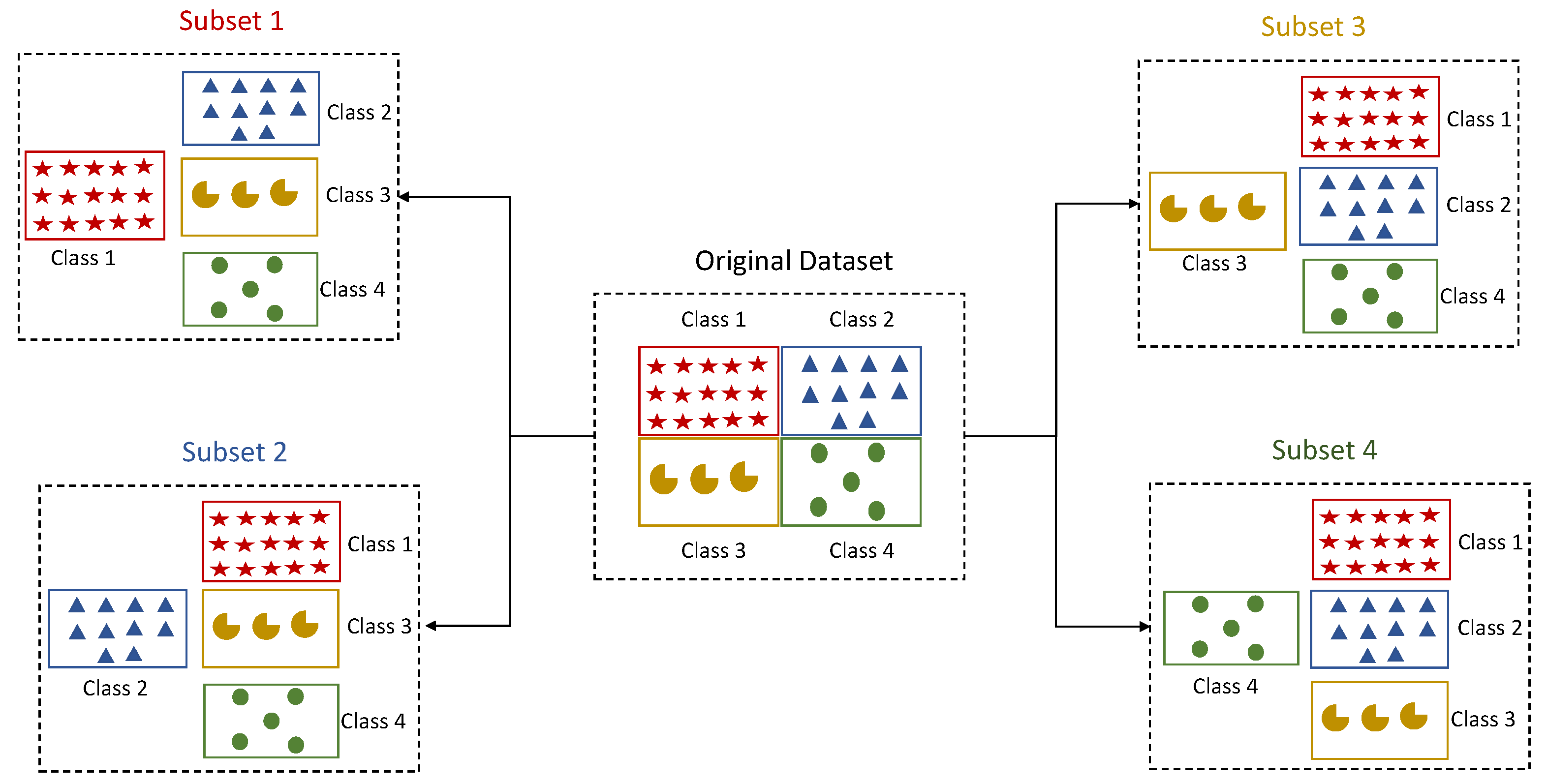
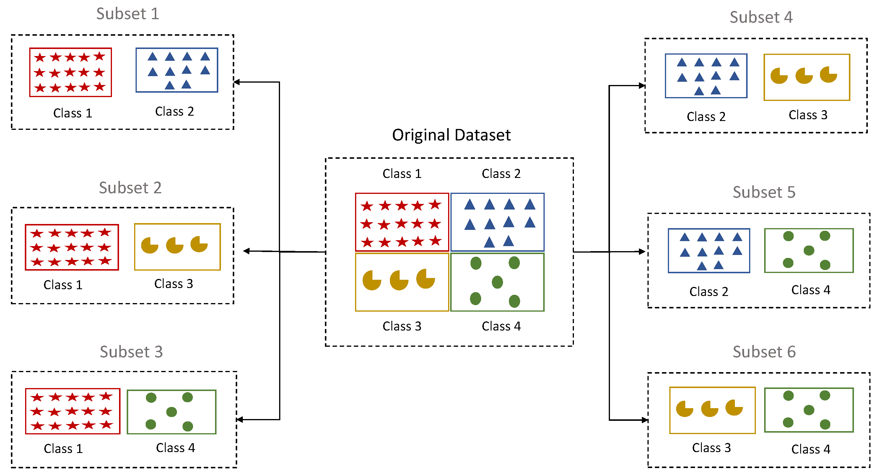
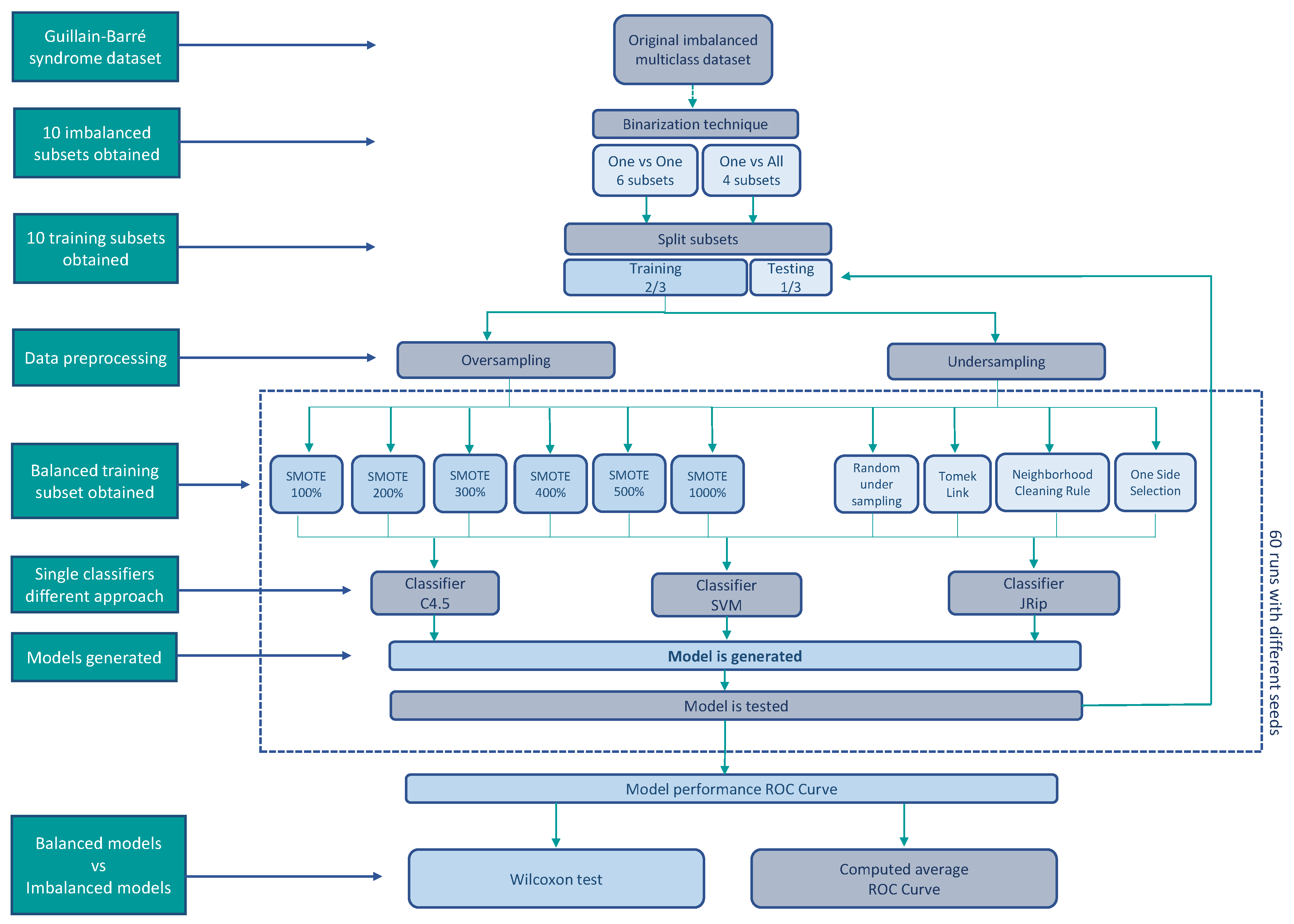
3.5. Binarization Techniques

In multiclass classification, it is common to decompose the original dataset containing all the classes into a binary dataset. One versus All (OVA) and One versus One (OVO) are two approaches commonly used for binarization. OVA and OVA facilitate the application of the data preprocessing techniques to balance the data before the training set goes to the classifier [60]. The OVA approach takes one class as a minority and the remaining classes are combined and transformed into the majority class. This procedure is made for the n classes of the dataset [61]. OVO trains a classifier for each possible pair of classes (n-1)/2 (pairwise learning) [62]. Figure 2 and Figure 3 show examples of OVA and OVO approaches used in a multiclass imbalanced dataset.

We use the OVA and OVO binarization technique widely used in classification problems [63]. From a medical perspective, OVA and OVO may assist physicians in distinguishing one subtype from another, an important task since each subtype varies in severity and treatment.

3.6. Validation

We used train-test evaluation for each single classifier, employing two-thirds of data for training, and one-third for testing.

4. Experimental Procedure

Figure 4 describes the experimental procedure. We tackle our multiclass classification problem by dividing it into two different binary subproblems using OVA and OVO approaches. Purple the sampling methods use binary datasets. These are integrated with minority class and majority class. For this reason, we used two different techniques to binarize our original GBS multiclass dataset. We created 10 binary datasets divided into two groups. purple The OVA technique takes a subtype of GBS which will be the minority class. The majority class will be made up of the sum of the other three remaining subtypes of GBS. Applying OVA, we obtained four imbalanced pairs of subsets. The OVO technique performs all possible combinations between two classes that integrated a dataset. For this experimental study, six possible imbalanced subsets pairs were obtained, created by the combination of the GBS subtypes from the original dataset.

Subsets obtained with OVA technique:

• GBS1 (129 instances): AIDP (20 instances) vs. ALL (109 instances).
• GBS2 (129 instances): AMAN (37 instances) vs. ALL (92 instances).
• GBS3 (129 instances): AMSAN (59 instances) vs. ALL (70 instances).
• GBS4 (129 instances): MF (13 instances) vs. ALL (116 instances).

Subsets obtained with OVO technique:

• GBS1 (57 instances): AIDP (20 instances) vs. AMAN (37 instances).
• GBS2 (79 instances): AIDP (20 instances) vs. AMSAN (59 instances).
• GBS3 (33 instances): AIDP (20 instances) vs. MF (13 instances).
• GBS4 (96 instances): AMAN (37 instances) vs. AMSAN (59 instances).
• GBS5 (50 instances): AMAN (37 instances) vs. MF (13 instances).
• GBS6 (72 instances): AMSAN (59 instances) vs. MF (13 instances).

We split each GBSn subset into two sets, 66% for training and 34% for testing. We balanced the training subsets applying sampling methods. The majority class of each training subset was under-sampled applying 4 different methods: Random Undersampling (RUS), Neighborhood Cleaning Rule (NCR), One Side Selection (OSS) and Tomek Link (TML). On the other hand, the minority class of the training subset was over-sampled using SMOTE at 100%, 200%, 300%, 400%, 500%, and 1000%, according to the literature [22,49].

Table 4. Majority class undersampling (OVA).

Subset	Original	Training	Random	Neighborhood	One Side	Tomek
			Undersampling	Cleaning Rule	Selection	Link
GBS1	109	73	14	62	63	67
GBS2	92	62	25	59	28	59
GBS3	70	47	40	41	24	43
GBS4	116	78	9	64	39	70

,

Table 5. Majority class undersampling (OVO).

Subset	Original	Training	Random	Neighborhood	One Side	Tomek
			Undersampling	Cleaning Rule	Selection	Link
GBS1	37	25	14	16	17	22
GBS2	59	40	14	35	14	38
GBS3	20	14	9	9	7	8
GBS4	59	40	25	39	16	39
GBS5	37	25	9	19	20	23
GBS6	59	40	9	34	35	37

,

Table 6. Minority class oversampling (OVA).

Subset	Original	Training	SMOTE	SMOTE	SMOTE	SMOTE	SMOTE	SMOTE
			100%	200%	300%	400%	500%	1000%
GBS1	20	14	28	42	56	70	84	154
GBS2	37	25	50	75	100	125	150	275
GBS3	59	40	80	120	160	200	240	440
GBS4	13	9	18	27	36	45	54	99

and

Table 7. Minority class oversampling (OVO).

Subset	Original	Training	SMOTE	SMOTE	SMOTE	SMOTE	SMOTE	SMOTE
			100%	200%	300%	400%	500%	1000%
GBS1	20	11	22	33	44	55	66	121
GBS2	20	14	28	42	56	70	84	154
GBS3	13	9	18	27	36	45	54	99
GBS4	37	24	48	72	96	120	144	264
GBS5	13	9	18	27	36	45	54	99
GBS6	13	10	20	30	40	50	60	110

shows results of data balancing.

We conducted 60 independent runs computing the ROC curve for each GBSn subset, and we obtained the average ROC curve. We performed this procedure for both imbalanced and balanced data using 3 different classifiers: C4.5, JRip, and SVM. Then, we compared imbalanced data models versus balanced data models. The model comparison was made using the Wilcoxon nonparametric test only when balanced data models outperformed imbalance data models.

We conducted a Wilcoxon test [64] to search for a statistical difference among the models using a significance value of 0.05. A nonparametric test was used since it does not require a particular data distribution [35].

Purple R is a language used to perform statistical analysis, it allows you to manipulate data quickly and accurately. R creates high-quality graphics, it is free and open source. It is an object-oriented language. RStudio is an IDE or integrated development environment. This means that RStudio is a program to manage R and use it more conveniently. RStudio includes a console, a syntax editor that supports code execution, as well as tools for plotting, debugging and managing the workspace. R experiments were performed in RStudio 1.2.1335.

A package is a collection of functions, data, and documentation that improves the capabilities of R. Packages are available in CRAN (Comprehensive R Archive Network). We used DMwR package [65] to oversampling with SMOTE. We used Unbalanced package to undersample the majority class with methods RUS, TML, OSS, NCL [66]. On the other hand, we applied three classifiers to create predictive models, using RWeka package [67] for C4.5 and JRip, e1071 package [68] for SVM classifier.

Other packages used were rJava [69], a low level interface for JAVA that allows the creation of objects. The data partition and the confusion matrix was created using the packagecaret [70]. To calculate the imbalance ratio we used imbalance [71]. Curve ROC was created using pROC [72]. We used lattice [73], for data viewer. We used rpart [74], a recursive partitioning for classification trees. To plot the models created by rpart we used rpart.plot [75]. SVM was tuned with the tune function, assigning the values 0.001, 0.01, 0.1, 1, 10, 50, 80, 100 for the C parameter.

5. Results and Discussion

This section show results obtained applying the four different undersampling techniques and the oversampling SMOTE technique to four imbalanced subsets obtained using OVA, as well as to six imbalanced subsets obtained using OVO. Each value is the average ROC curve obtained across 60 runs, each with a different seed.

We applied C4.5, SVM and JRip classifiers after the data balancing and we evaluated the model performance using ROC, the most accepted metric for imbalanced problems. We used the Wilcoxon test to evaluate the statistically significant difference between the models using imbalanced data against to the models using balanced data.

In

Table 8. Imbalance Ratio for OVA.

SGB	Minority	Majority	Imbalance
	Class	Class	Ratio
GBS1	20	109	5.4500
GBS2	37	92	2.4865
GBS3	59	70	1.1864
GBS4	13	116	8.9231

and

Table 9. Imbalance Ratio for OVO.

SGB	Minority	Majority	Imbalance
	Class	Class	Ratio
GBS1	20	37	1.8500
GBS2	20	59	2.9500
GBS3	13	20	1.5385
GBS4	37	59	1.5946
GBS5	13	37	2.8462
GBS6	13	59	4.5385

, we show the $IR$ computed of the GBS subset from OVA and OVO. The highest $IR$ values were obtained with OVA. This is because the higher the number of the majority class with respect to the minority one the higher the result. However, in GBS3 the $IR=1.1864$. Some authors consider that a dataset is imbalanced when $IR>1$ [76]. For OVO, in all cases, $IR>1.5$.

Table 10. Comparison between imbalanced data and balanced data using four undersampling methods. The values are average classification results across 60 runs using OVA.

Case Instances	Classifier	Imbalanced Dataset	Random Undersampling	Wilcoxon Test	Tomek Link	Wilcoxon Test	One Side Selection	Wilcoxon Test	Neighborhood Cleaning Rule	Wilcoxon Test
		ROC	ROC	RESULT	ROC	RESULT	ROC	RESULT	ROC	RESULT
GBS1	C4.5	0.8130	0.7940	NC	0.8287	$\mathcal{NS}$	0.8192	$\mathcal{NS}$	0.8273	$\mathcal{NS}$
AIDP-ALL	SVM	0.7477	0.7734	$\mathcal{NS}$	0.7553	$\mathcal{NS}$	0.7618	$\mathcal{NS}$	0.7632	$\mathcal{NS}$
20-109	JRip	0.7826	0.8150 *	$\mathcal{S}$	0.7949	$\mathcal{NS}$	0.7766	NC	0.8074 *	$\mathcal{S}$
SGB2	C4.5	0.9003	0.8924	NC	0.9088	$\mathcal{NS}$	0.9182 *	$\mathcal{S}$	0.8939	NC
AMAN-ALL	SVM	0.8594	0.8832 *	$\mathcal{S}$	0.8575	NC	0.8611	$\mathcal{NS}$	0.8557	NC
37-92	JRip	0.8608	0.8656	$\mathcal{NS}$	0.8668	$\mathcal{NS}$	0.8601	NC	0.8414	NC
SGB3	C4.5	0.8632	0.8582	NC	0.8579	NC	0.8496	NC	0.8644	$\mathcal{NS}$
AMSAN-ALL	SVM	0.7898	0.7906	$\mathcal{NS}$	0.7911	$\mathcal{NS}$	0.7870	NC	0.7981	$\mathcal{NS}$
59-70	JRip	0.8470	0.8440	NC	0.8639	NC	0.8288	NC	0.8444	NC
SGB4	C4.5	0.7662	0.8906 *	$\mathcal{S}$	0.7935	$\mathcal{NS}$	0.8103 *	$\mathcal{S}$	0.8033	$\mathcal{NS}$
MF-ALL	SVM	0.6846	0.7099	$\mathcal{NS}$	0.7323	$\mathcal{NS}$	0.7709 *	$\mathcal{S}$	0.7319	$\mathcal{NS}$
13-116	JRip	0.8319	0.8781 *	$\mathcal{S}$	0.8577	$\mathcal{NS}$	0.8633	$\mathcal{NS}$	0.8498	$\mathcal{NS}$

NC = Not computed; $\mathcal{NS}$ = Not significant; $\mathcal{S}$ = Significant.

,

Table 11. Comparison between imbalanced data and balanced data using 4 undersampling methods. The values are average classification results across 60 runs using OVO.

Case Instaces	Classifier	Imbalanced Dataset	Random Undersampling	Wilcoxon Test	Tomek Link	Wilcoxon Test	One Side Selection	Wilcoxon Test	Neighborhood Cleaning Rule	Wilcoxon Test
		ROC	ROC	RESULT	ROC	RESULT	ROC	RESULT	ROC	RESULT
GBS1	C4.5	0.9604	0.9264	NC	0.9319	NC	0.8972	NC	0.9458	NC
AIDP-AMAN	SVM	0.9674	0.9639	NC	0.9590	NC	0.9528	NC	0.9660	NC
20-37	JRip	0.9563	0.9479	NC	0.9500	NC	0.9146	NC	0.9438	NC
GBS2	C4.5	0.8585	0.8251	NC	0.8541	NC	0.8266	NC	0.8496	NC
AIDP-AMSAN	SVM	0.8490	0.8292	NC	0.8458	NC	0.8242	NC	0.8447	NC
20-59	JRip	0.8260	0.8220	NC	0.8308	$\mathcal{NS}$	0.8471	$\mathcal{NS}$	0.8289	$\mathcal{NS}$
GBS3	C4.5	0.8132	0.8667 *	$\mathcal{S}$	0.8840 *	$\mathcal{S}$	0.8854 *	$\mathcal{S}$	0.8604 *	$\mathcal{S}$
AIDP-MF	SVM	0.7097	0.6465	NC	0.6667	NC	0.6354	NC	0.6542	NC
20-13	JRip	0.8556	0.8757	$\mathcal{NS}$	0.8771	$\mathcal{NS}$	0.8590	$\mathcal{NS}$	0.8507	$\mathcal{NS}$
GBS4	C4.5	0.9258	0.9102	NC	0.9270	$\mathcal{NS}$	0.9260	$\mathcal{NS}$	0.9178	NC
AMAN-AMSAN	SVM	0.8783	0.8976 *	$\mathcal{S}$	0.8721	NC	0.8647	NC	0.8823	$\mathcal{NS}$
37-59	JRip	0.8782	0.8966	$\mathcal{NS}$	0.8973 *	$\mathcal{S}$	0.9098 *	$\mathcal{S}$	0.8758	NC
GBS5	C4.5	0.8736	0.8813	$\mathcal{NS}$	0.8847	$\mathcal{NS}$	0.8632	NC	0.8847	$\mathcal{NS}$
AMAN-MF	SVM	0.8910	0.8743	NC	0.8840	NC	0.8569	NC	0.8785	NC
37-13	JRip	0.8854	0.8736	NC	0.8792	NC	0.8771	NC	0.8854	NC
GBS6	C4.5	0.8007	0.8753 *	$\mathcal{S}$	0.8679 *	$\mathcal{S}$	0.8582 *	$\mathcal{S}$	0.8401 *	$\mathcal{S}$
AMSAN-MF	SVM	0.7388	0.7724	$\mathcal{NS}$	0.7784 *	$\mathcal{S}$	0.7538	$\mathcal{NS}$	0.7701	$\mathcal{NS}$
59-13	JRip	0.8580	0.8811	$\mathcal{NS}$	0.8635	$\mathcal{NS}$	0.8640	$\mathcal{NS}$	0.8385	NC

NC = Not computed; $\mathcal{NS}$ = Not significant; $\mathcal{S}$ = Significant.

,

Table 12. Comparison between imbalanced data and balanced data using SMOTE method. The values are average classification results across 60 runs using OVA.

Case Instances	Classifier	Imbalanced Dataset	SMOTE 100%	Wilcoxon Test	SMOTE 200%	Wilcoxon Test	SMOTE 300%	Wilcoxon Test	SMOTE 400%	Wilcoxon Test	SMOTE 500%	Wilcoxon Test	SMOTE 1000%	Wilcoxon Test
		ROC	ROC	RESULT	ROC	RESULT	ROC	RESULT	ROC	RESULT	ROC	RESULT	ROC	RESULT
GBS1	C4.5	0.8130	0.8042	NC	0.7951	NC	0.7905	NC	0.7986	NC	0.7877	NC	0.7951	NC
AIDP-ALL	SVM	0.7477	0.7750	$\mathcal{NS}$	0.7544	$\mathcal{NS}$	0.7407	NC	0.7498	$\mathcal{NS}$	0.7428	NC	0.7556	$\mathcal{NS}$
20-109	JRip	0.7826	0.8102 *	$\mathcal{S}$	0.7993	$\mathcal{NS}$	0.8030 *	$\mathcal{S}$	0.8046	$\mathcal{NS}$	0.7891	$\mathcal{NS}$	0.7993	$\mathcal{NS}$
GBS2	C4.5	0.9003	0.8900	NC	0.8972	NC	0.8915	NC	0.8890	NC	0.8890	NC	0.8939	NC
AMAN-ALL	SVM	0.8594	0.8490	NC	0.8417	NC	0.8411	NC	0.8401	NC	0.8417	NC	0.8379	NC
37-92	JRip	0.8608	0.8699	$\mathcal{NS}$	0.8718	$\mathcal{NS}$	0.8606	$\mathcal{NC}$	0.8689	$\mathcal{NS}$	0.8892 *	$\mathcal{S}$	0.8767	$\mathcal{NS}$
GBS3	C4.5	0.8632	0.8795 *	$\mathcal{S}$	0.8592	$\mathcal{NC}$	0.8689	$\mathcal{NS}$	0.8699	$\mathcal{NS}$	0.8747	$\mathcal{NS}$	0.8792	$\mathcal{NS}$
AMSAN-ALL	SVM	0.7898	0.7881	NC	0.7863	NC	0.7888	NC	0.7909	$\mathcal{NS}$	0.7917	$\mathcal{NS}$	0.7887	NC
59-70	JRip	0.8470	0.8442	NC	0.8603 *	$\mathcal{S}$	0.8640 *	$\mathcal{S}$	0.8632	$\mathcal{NS}$	0.8616 *	$\mathcal{S}$	0.8678 *	$\mathcal{S}$
GBS4	C4.5	0.7662	0.8951 *	$\mathcal{S}$	0.8588 *	$\mathcal{S}$	0.8292 *	$\mathcal{S}$	0.8180	$\mathcal{NS}$	0.8340 *	$\mathcal{S}$	0.8007	$\mathcal{NS}$
MF-ALL	SVM	0.6846	0.7516 *	$\mathcal{S}$	0.7590 *	$\mathcal{S}$	0.7409	$\mathcal{NS}$	0.7568 *	$\mathcal{S}$	0.7604 *	$\mathcal{S}$	0.7679 *	$\mathcal{S}$
13-116	JRip	0.8319	0.8826 *	$\mathcal{S}$	0.8447	$\mathcal{NS}$	0.8339	$\mathcal{NS}$	0.8466	$\mathcal{NS}$	0.8469	$\mathcal{NS}$	0.8198	NC

NC = Not computed; $\mathcal{NS}$ = Not significant; $\mathcal{S}$ = Significant.

and

Table 13. Comparison between imbalanced data and balanced data using SMOTE method. The values are average classification results across 60 runs using OVO.

Case Instances	Classifier	Imbalanced Dataset	SMOTE 100%	Wilcoxon Test	SMOTE 200%	Wilcoxon Test	SMOTE 300%	Wilcoxon Test	SMOTE 400%	Wilcoxon Test	SMOTE 500%	Wilcoxon Test	SMOTE 1000%	Wilcoxon Test
		ROC	ROC	RESULT	ROC	RESULT	ROC	RESULT	ROC	RESULT	ROC	RESULT	ROC	RESULT
GBS1	C4.5	0.9563	0.9576	$\mathcal{NS}$	0.9438	NC	0.9493	NC	0.9528	NC	0.9556	NC	0.9576	$\mathcal{NS}$
AIDP-AMAN	SVM	0.9618	0.9618	NC	0.9632	NC	0.9639	NC	0.9625	NC	0.9632	NC	0.9632	NC
20-37	JRip	0.9507	0.9403	NC	0.9424	NC	0.9403	NC	0.9382	NC	0.9319	NC	0.9389	NC
GBS2	C4.5	0.8656	0.8551	NC	0.8485	NC	0.8375	NC	0.8502	NC	0.8607	NC	0.8551	NC
AIDP-AMSAN	SVM	0.8557	0.8333	NC	0.8328	NC	0.8428	NC	0.8381	NC	0.8338	NC	0.8333	NC
20-59	JRip	0.8472	0.8549	$\mathcal{NS}$	0.8285	NC	0.8480	$\mathcal{NS}$	0.8561	$\mathcal{NS}$	0.8480	$\mathcal{NS}$	0.8549	$\mathcal{NS}$
GBS3	C4.5	0.8132	0.7965	NC	0.7986	NC	0.7889	NC	0.7729	NC	0.7958	NC	0.7965	NC
AIDP-MF	SVM	0.7097	0.6535	NC	0.6486	NC	0.6472	NC	0.6465	NC	0.6563	NC	0.6535	NC
20-13	JRip	0.8458	0.7382	NC	0.7778	NC	0.7750	NC	0.7646	NC	0.7292	NC	0.7382	NC
GBS4	C4.5	0.9132	0.9093	NC	0.9096	NC	0.9172	$\mathcal{NS}$	0.9062	NC	0.9207	$\mathcal{NS}$	0.9093	NC
MF-ALL	SVM	0.8863	0.8827	NC	0.8844	NC	0.8843	NC	0.8840	NC	0.8821	NC	0.8827	NC
13-116	JRip	0.8809	0.9065 *	$\mathcal{S}$	0.9042 *	$\mathcal{S}$	0.9019 *	$\mathcal{S}$	0.9043 *	$\mathcal{S}$	0.9071 *	$\mathcal{S}$	0.9065 *	$\mathcal{S}$
GBS5	C4.5	0.8736	0.8868	$\mathcal{NS}$	0.8792	$\mathcal{NS}$	0.8833	$\mathcal{NS}$	0.8701	NC	0.8861	$\mathcal{NS}$	0.8868	$\mathcal{NS}$
AMAN-NF	SVM	0.8910	0.8847	NC	0.8715	NC	0.8792	NC	0.8840	NC	0.8847	NC	0.8847	NC
37-13	JRip	0.8799	0.8889	$\mathcal{NS}$	0.8799	NC	0.8875	$\mathcal{NS}$	0.8903	$\mathcal{NS}$	0.8861	$\mathcal{NS}$	0.8889	$\mathcal{NS}$
GBS6	C4.5	0.8007	0.7839	NC	0.8185	$\mathcal{NS}$	0.8287	$\mathcal{NS}$	0.8084	$\mathcal{NS}$	0.8041	$\mathcal{NS}$	0.7839	NC
AMSAN-MF	SVM	0.7388	0.7534	$\mathcal{NS}$	0.7646	$\mathcal{NS}$	0.7651	$\mathcal{NS}$	0.7522	$\mathcal{NS}$	0.7469	$\mathcal{NS}$	0.7534	$\mathcal{NS}$
59-13	JRip	0.8430	0.8720 *	$\mathcal{S}$	0.8393	NC	0.8306	NC	0.8213	NC	0.8111	NC	0.8061	NC

NC = Not computed; $\mathcal{NS}$ = Not significant; $\mathcal{S}$ = Significant.

show in bold the cases with a statistically significant difference. The structure of the four tables is as follows: first column shows the subsets obtained using binarization techniques (OVA, OVO), the GBS subtype included, as well as the number of instances for each of them. The second column shows the three classifiers used for each subset. The third column shows the results of the classifiers using the imbalanced data.

Subsequent columns show results of applying the balance techniques and their corresponding Wilcoxon test, where $\mathcal{NS}$ (Not Significant) stands for a not statistically significant difference between results using imbalanced data and results using balanced data, NC (Not Computed) means that the test could not be performed due to many identical results across the 60 runs or that best results were obtained using imbalanced data, and $\mathcal{S}$ (Significant) represents that there is a statistically significant difference between results using imbalanced data against to balanced data.

Table 10 shows results obtained after applying RUS, TML, OSS, and NCR to the four imbalanced subsets obtained through OVA. A total of 48 data balanced cases were obtained. In 16 cases, balanced data could not improve imbalanced data. In 24 cases, balanced data improved the imbalanced data with no statistically significant difference. Eight cases presented a statistically significant difference. These cases are listed below with their corresponding ROC value.

$$\begin{array}{lll}GBS{1}_{\mathtt{RUS}/\mathtt{JRIP}}^{\mathit{OVA}}=0.8150& GBS{2}_{\mathit{RUS}/\mathit{SVM}}^{\mathtt{OVA}}=0.8832& GBS{4}_{\mathit{RUS}/\mathit{JRIP}}^{\mathtt{OVA}}=0.8781\\ GBS{1}_{\mathit{NCR}/\mathit{JRIP}}^{\mathtt{OVA}}=0.8074& GBS{4}_{\mathit{RUS}/\mathit{C}4.5}^{\mathtt{OVA}}=0.8906& GBS{4}_{\mathit{OSS}/\mathit{SVM}}^{\mathtt{OVA}}=0.7709\\ GBS{2}_{\mathit{OSS}/\mathit{C}4.5}^{\mathtt{OVA}}=0.9182& GBS{4}_{\mathit{OSS}/\mathit{C}4.5}^{\mathtt{OVA}}=0.8103& \end{array}$$

GBS4 subset obtained the best results. In all 12 cases, the balanced data improved the imbalanced data, applying all four undersampling methods and all three classifiers. Furthermore, a statistically significant difference was found in four of them. GBS3 subset obtained the worst performance. Balanced data could not improve the imbalanced data in eight cases. Balanced data improved imbalanced data only in four cases, with no statistically significant difference.

The best undersampling method using OVA was RUS because it improved imbalanced data in 8 cases, half of them with a statistically significant difference. OSS improved results in seven cases, three of them with a statistically significant difference. NCR improved imbalanced data in 8 cases, however, only one of them obtained a statistically significant difference. TML obtained the worst performance, although in nine cases results were improved, none of them obtained a statistically significant difference.

We conducted 16 experiments cases for each classifier, derived from applying four undersampling methods in 4GBS subsets. From these experiments, C4.5 obtained the best results, in 11 cases balanced data improved imbalanced data, three of them with a statistically significant difference. Applying SVM, in 13 cases balanced data improved imbalanced data, but only two of them with a statistically significant difference. Finally with JRip, in nine cases balanced data improved imbalanced data, three of them with a statistically significant difference.

Table 11 shows results obtained after applying RUS, TML, OSS and NCR to the 6 imbalanced subsets obtained through OVO. A total of 72 data balanced cases were obtained. In 40 cases, balanced data could not improve imbalanced data. In 20 cases, balanced data improved the imbalanced data with no statistically significant difference. 12 cases presented a statistically significant difference. These cases are listed below with their corresponding ROC value.

$$\begin{array}{lll}GBS{3}_{\mathit{RUS}/\mathit{C}4.5}^{\mathtt{OVO}}=0.8667& GBS{4}_{\mathit{RUS}/\mathit{SVM}}^{\mathtt{OVO}}=0.8976& GBS{6}_{\mathit{OSS}/\mathit{C}4.5}^{\mathtt{OVO}}=0.8582\\ GBS{3}_{\mathit{OSS}/\mathit{C}4.5}^{\mathtt{OVO}}=0.8854& GBS{4}_{\mathit{OSS}/\mathit{JRip}}^{\mathtt{OVO}}=0.9098& GBS{6}_{\mathit{TML}/\mathit{SVM}}^{\mathtt{OVO}}=0.7784\\ GBS{3}_{\mathit{NCR}/\mathit{C}4.5}^{\mathtt{OVO}}=0.8604& GBS{4}_{\mathit{TML}/\mathit{JRip}}^{\mathtt{OVO}}=0.8973& GBS{6}_{\mathit{TML}/\mathit{C}4.5}^{\mathtt{OVO}}=0.8679\\ GBS{3}_{\mathit{TML}/\mathit{C}4.5}^{\mathtt{OVO}}=0.8840& GBS{6}_{\mathit{RUS}/\mathit{C}4.5}^{\mathtt{OVO}}=0.8753& GBS{6}_{\mathit{NCR}/\mathit{C}4.5}^{\mathtt{OVO}}=0.8401\end{array}$$

GBS6 subset obtained the best results. In 11 out of 12 cases the balanced data improved the imbalanced data, 5 of them with a statistically significant difference. In only one case the balanced data could not improve the imbalanced data. GBS1 subset had the worst performance. In none of the 12 cases, the balanced data improved the imbalanced data.

The best undersampling method using OVO was TML since it improved imbalanced data in 9 cases, in 4 of them with statistically significant difference. RUS and OSS behaved the same, that is, in 8 cases the balanced data improved the imbalanced data, 3 of them with a statistically significant difference. NCR had the worst performance: in 7 cases the balanced data improved the imbalanced data, 2 of them with a statistically significant difference.

We conducted 16 experiments for each classifier, as in OVA. From these experiments, C4.5 obtained the best results, in 13 cases the balanced data improved the imbalanced data, 8 of them with a statistically significant difference. Applying JRip, in 13 cases the balanced data improved the imbalanced data but only 2 of them with a statistically significant difference. With SVM, in 6 cases the balanced data improved the imbalanced data, 2 of them with a statistically significant difference.

Table 12 shows results obtained after applying SMOTE at 100%, 200%, 300%, 400%, 500%, and 1000% to the 4 imbalanced subsets obtained through OVA. A total of 72 data balanced cases were obtained as result from applying three classifiers to 24 imbalanced subsets. In 28 cases, balanced data could not improve imbalanced data. In 26 cases, balanced data improved the imbalanced data with no statistically significant difference. 18 cases presented a statistically significant difference. These cases are listed below with their corresponding ROC value.

$$\begin{array}{lll}GBS{1}_{\mathit{SMT}100/\mathit{JRip}}^{\mathtt{OVA}}=0.8102& GBS{3}_{\mathit{SMT}500/\mathit{JRip}}^{\mathtt{OVA}}=\mathrm{=\; 0.8616}& GBS{4}_{\mathit{SMT}100/\mathit{SVM}}^{\mathtt{OVA}}=0.7516\\ GBS{1}_{\mathit{SMT}300/\mathit{JRip}}^{\mathtt{OVA}}=0.8030& GBS{3}_{\mathit{SMT}1000/\mathit{JRip}}^{\mathtt{OVA}}=0.8678& GBS{4}_{\mathit{SMT}200/\mathit{SVM}}^{\mathtt{OVA}}=0.7590\\ GBS{2}_{\mathit{SMT}500/\mathit{JRip}}^{\mathtt{OVA}}=0.8892& GBS{4}_{\mathit{SMT}100/\mathit{C}4.5}^{\mathtt{OVA}}=0.8951& GBS{4}_{\mathit{SMT}400/\mathit{SVM}}^{\mathtt{OVA}}=0.7568\\ GBS{3}_{\mathit{SMT}100/\mathit{C}4.5}^{\mathtt{OVA}}=0.8795& GBS{4}_{\mathit{SMT}200/\mathit{C}4.5}^{\mathtt{OVA}}=0.8588& GBS{4}_{\mathit{SMT}500/\mathit{SVM}}^{\mathtt{OVA}}=0.7604\\ GBS{3}_{\mathit{SMT}200/\mathit{JRip}}^{\mathtt{OVA}}=0.8603& GBS{4}_{\mathit{SMT}300/\mathit{C}4.5}^{\mathtt{OVA}}=0.8292& GBS{4}_{\mathit{SMT}1000/\mathit{SVM}}^{\mathtt{OVA}}=0.7679\\ GBS{3}_{\mathit{SMT}300/\mathit{JRip}}^{\mathtt{OVA}}=0.8640& GBS{4}_{\mathit{SMT}500/\mathit{C}4.5}^{\mathtt{OVA}}=0.8340& GBS{4}_{\mathit{SMT}100/\mathit{JRip}}^{\mathtt{OVA}}=0.8826\end{array}$$

GBS4 subset obtained the best results. From 18 balancing cases with SMOTE, in only one case balanced data could no improve imbalanced data. In 7 cases, balanced data improved imbalanced data without a statistically significant difference. In 10 cases, a statistically significant difference was found. On the other hand, GBS2 obtained the worst performance. In only one case a statistically significant difference was found. In 4 cases, balanced data improved imbalanced data; however, a statistically significant difference was not found. In 13 cases, balanced data could no improve imbalanced data.

For OVA and SMOTE techniques, the best performance was obtained applying SMOTE at 100%, since in seven cases balanced data improved the imbalanced data, 5 of them with a statistically significant differences. SMOTE at 400% obtained the worst performance since in 9 cases balanced data improved the imbalanced data, however, only one obtained a statistically significant difference.

As for the classifiers, JRip obtained the best performance, given that in 13 cases balanced data improved imbalanced data without statistically significant difference. In addition, in other 8 cases we found a statistically significant difference. With C4.5, in 11 cases balanced data improved imbalanced data, however, only 5 of them obtained a statistically significant difference. Applying SVM, in 12 cases balanced data improved imbalanced data, but only 5 of them with a statistically significant difference.

We conclude that SMOTE at 100% combined with JRip obtained best results.

Table 13 shows results obtained after applying SMOTE at 100%, 200%, 300%, 400%, 500%, and 1000% to the 6 imbalanced subsets obtained through OVO. A total of 108 data balanced cases were obtained as result from applying 3 classifier to 36 imbalanced subsets. In 72 cases, balanced data could not improve imbalanced data. In 29 cases, balanced data improved the imbalanced data with no a statistically significant difference. 7 cases presented a statistically significant difference. These cases are listed below with their corresponding ROC value.

$$\begin{array}{lll}GBS{4}_{\mathit{SMT}100/\mathit{JRip}}^{\mathtt{OVO}}=0.9065& GBS{4}_{\mathit{SMT}400/\mathit{JRip}}^{\mathtt{OVO}}=0.9043& GBS{6}_{\mathit{SMT}100/\mathit{JRip}}^{\mathtt{OVO}}=0.8720\\ GBS{4}_{\mathit{SMT}200/\mathit{JRip}}^{\mathtt{OVO}}=0.9042& GBS{4}_{\mathit{SMT}500/\mathit{JRip}}^{\mathtt{OVO}}=0.9071& \\ GBS{4}_{\mathit{SMT}300/\mathit{JRip}}^{\mathtt{OVO}}=0.9019& GBS{4}_{\mathit{SMT}1000/\mathit{JRip}}^{\mathtt{OVO}}=0.9065& \end{array}$$

GBS4 subset obtained the best results. In 6 cases, a statistically significant difference was found. In 2 cases, balanced data improved the imbalanced data with no statistically significant difference. In 10 cases, balanced data could not improve the imbalanced data. GBS3 subset obtained the worst performance. In all 18 cases, balanced data could not improve the imbalanced data.

For OVO and SMOTE techniques, the best performance was obtained applying SMOTE at 100%, since in 5 cases, balanced data improved the imbalanced data without a statistically significant difference, however, in 2 cases a statistically significant difference was found. In 11 cases, balanced data could no improve the imbalanced data. SMOTE at 400% obtained the worst performance since in 14 cases balanced data could no improve the imbalanced data. In 4 cases, balanced data improved the imbalanced data, however, only one case obtained a statistically significant difference.

As for the classifiers, JRip obtained the best performance. In 8 cases balanced data improved the imbalanced data with no statistically significant difference, however, in 6 cases we founded a statistically significant difference. In 16 cases balanced data could no improve the imbalanced data. Applying C4.5, in 19 cases balanced data could no improve the imbalanced data, in 11 cases balanced data improved the imbalanced data, without a statistically significant difference. SVM obtained worst performance, only in 5 cases balanced data improved the imbalanced data, however, a statistically significant difference was not found.

We conclude, as in OVA, for OVO and SMOTE at 100% combined with JRip obtained the best results.

6. Conclusions

The aim of this work was to investigate if balancing the original GBS dataset improves the predictive models to identify GBS subtypes created in a previous study. We performed 4 independent experiments applying data-level techniques.

We started by creating 10 binary datasets divided into two groups. We used OVA and OVO techniques on the original dataset obtaining 4 and 6 binary subsets respectively. We divided each GBSn subset into 2 sets, 66% for training and 34% for testing. We balanced the training subset using two sampling methods. The majority class for each training subset was undersampled applying 4 different methods: RUS, NCR, OSS, and TML. Furthermore, the minority class of the training subset was oversampled applying SMOTE at 100%, 200%, 300%, 400%, 500%, and 1000%. Undersampling and oversampling were applied for OVA and OVO.

Once the training subsets were balanced, we applied 3 different classifiers: C4.5, JRip, and SVM. The scores are the average ROC curve obtained through 60 runs, each with a different seed. We used the Wilcoxon test to assess whether there is a statistically significant difference between the imbalanced models versus the balanced models.

The number of cases with statistically significant difference between imbalanced data and balanced data across the 4 experiments was: 8 for OVA with undersampling, 12 for OVO with undersampling, 18 for OVA with SMOTE, and 7 for OVO with SMOTE.

From all 4 sampling experiments, the best results were obtained combining SMOTE with OVA. Regarding classifiers, JRip obtained the best performance since it found more cases with statistically significant differences for all experiments.

Purple Balance a subset data using oversampling obtained better performance. Adding synthetic instances to minority class applying SMOTE helped classifiers get the best performance. On the other hand, eliminating instances of the majority class resulted in losing information that the classifiers needed to achieve better performance. However, factors independent of imbalanced data, such as noise, can affect the performance of the classifiers. We found that the best results were obtained in the combinations where the majority class clearly exceeds the minority class. In these cases, the instances clearly distinguish each other and the undersampling algorithms were only responsible for eliminating noise or class overlapping that helped improve the performance of the classifiers. On the contrary, when the classes have a similar number of instances, the worst results were produced.

The results achieved in this research shows that balancing the original dataset improves the previous predictive models. In addition, this predictive model can help specialists to identify the subtype of GBS that a patient suffers. Early identification of the subtype will allow starting with the appropriate treatment for patient recovery. This is a contribution to exploring the performance of balancing techniques with real data.

As future work, we will experiment with different variants of SMOTE, and we will apply a hybrid approach using the OVA and OVO techniques. Also, we plan to build more accurate predictive models using different single and ensemble methods.

References

1. Abbassi, N.; Ambegaonkar, G. Guillain-Barre syndrome: A review. Paediatr. Child Health 2019, 29, 459–462. [Google Scholar] [CrossRef]
2. Elettreby, M.F.; Ahmed, E.; Safan, M. A simple mathematical model for Guillain–Barré syndrome. Adv. Differ. Equations 2019, 2019. [Google Scholar] [CrossRef]
3. Pinto-Díaz, C.A.; Rodríguez, Y.; Monsalve, D.M.; Acosta-Ampudia, Y.; Molano-González, N.; Anaya, J.M.; Ramírez-Santana, C. Autoimmunity in Guillain-Barré syndrome associated with Zika virus infection and beyond. Autoimmun. Rev. 2017, 16, 327–334. [Google Scholar] [CrossRef] [PubMed]
4. Kuwabara, S. Guillain-Barr?? Syndrome. Drugs 2004, 64, 597–610. [Google Scholar] [CrossRef]
5. Panesar, K. Guillain-Barré Syndrome. US Pharm. 2014, 39, 35–38. [Google Scholar]
6. Rodríguez, Y.; Chang, C.; González-Bravo, D.C.; Gershwin, M.E.; Anaya, J.M. Guillain-Barré Syndrome. In Neuroimmune Diseases; Springer International Publishing: Basel, Switzerland, 2019; pp. 711–736. [Google Scholar] [CrossRef]
7. Abdi, L.; Hashemi, S. To combat multi-class imbalanced problems by means of over-sampling and boosting techniques. Soft Comput. 2014, 19, 3369–3385. [Google Scholar] [CrossRef]
8. He, H.; Garcia, E. Learning from Imbalanced Data. IEEE Trans. Knowl. Data Eng. 2009, 21, 1263–1284. [Google Scholar] [CrossRef]
9. Sáez, J.A.; Krawczyk, B.; Woźniak, M. Analyzing the oversampling of different classes and types of examples in multi-class imbalanced datasets. Pattern Recognit. 2016, 57, 164–178. [Google Scholar] [CrossRef]
10. Feng, W.; Huang, W.; Ren, J. Class Imbalance Ensemble Learning Based on the Margin Theory. Appl. Sci. 2018, 8, 815. [Google Scholar] [CrossRef] [Green Version]
11. Guo, H.; Zhou, J.; Wu, C.A. Imbalanced Learning Based on Data-Partition and SMOTE. Information 2018, 9, 238. [Google Scholar] [CrossRef] [Green Version]
12. Lee, P. Resampling Methods Improve the Predictive Power of Modeling in Class-Imbalanced Datasets. Int. J. Environ. Res. Public Health 2014, 11, 9776–9789. [Google Scholar] [CrossRef] [PubMed] [Green Version]
13. Canul-Reich, J.; Frausto-Solís, J.; Hernández-Torruco, J. A Predictive Model for Guillain-Barré Syndrome Based on Single Learning Algorithms. Comput. Math. Methods Med. 2017, 2017, 1–9. [Google Scholar] [CrossRef] [PubMed] [Green Version]
14. Canul-Reich, J.; Hernández-Torruco, J.; Chávez-Bosquez, O.; Hernández-Ocaña, B. A Predictive Model for Guillain–Barré Syndrome Based on Ensemble Methods. Comput. Intell. Neurosci. 2018, 2018, 1–10. [Google Scholar] [CrossRef] [PubMed]
15. Han, W.; Huang, Z.; Li, S.; Jia, Y. Distribution-Sensitive Unbalanced Data Oversampling Method for Medical Diagnosis. J. Med. Syst. 2019, 43. [Google Scholar] [CrossRef] [PubMed]
16. Bach, M.; Werner, A.; Żywiec, J.; Pluskiewicz, W. The study of under- and over-sampling methods’ utility in analysis of highly imbalanced data on osteoporosis. Inf. Sci. 2017, 384, 174–190. [Google Scholar] [CrossRef]
17. Kalwa, U.; Legner, C.; Kong, T.; Pandey, S. Skin Cancer Diagnostics with an All-Inclusive Smartphone Application. Symmetry 2019, 11, 790. [Google Scholar] [CrossRef] [Green Version]
18. Le, T.; Baik, S. A Robust Framework for Self-Care Problem Identification for Children with Disability. Symmetry 2019, 11, 89. [Google Scholar] [CrossRef] [Green Version]
19. Ijaz, M.; Alfian, G.; Syafrudin, M.; Rhee, J. Hybrid Prediction Model for Type 2 Diabetes and Hypertension Using DBSCAN-Based Outlier Detection, Synthetic Minority Over Sampling Technique (SMOTE), and Random Forest. Appl. Sci. 2018, 8, 1325. [Google Scholar] [CrossRef] [Green Version]
20. Elreedy, D.; Atiya, A.F. A Comprehensive Analysis of Synthetic Minority Oversampling Technique (SMOTE) for handling class imbalance. Inf. Sci. 2019, 505, 32–64. [Google Scholar] [CrossRef]
21. Devi, D.; kr. Biswas, S.; Purkayastha, B. Redundancy-driven modified Tomek-link based undersampling: A solution to class imbalance. Pattern Recognit. Lett. 2017, 93, 3–12. [Google Scholar] [CrossRef]
22. Bach, M.; Werner, A.; Palt, M. The Proposal of Undersampling Method for Learning from Imbalanced Datasets. Procedia Comput. Sci. 2019, 159, 125–134. [Google Scholar] [CrossRef]
23. Vuttipittayamongkol, P.; Elyan, E. Neighbourhood-based undersampling approach for handling imbalanced and overlapped data. Inf. Sci. 2020, 509, 47–70. [Google Scholar] [CrossRef]
24. Kovács, G. An empirical comparison and evaluation of minority oversampling techniques on a large number of imbalanced datasets. Appl. Soft Comput. 2019, 83, 105662. [Google Scholar] [CrossRef]
25. Gosain, A.; Sardana, S. Farthest SMOTE: A Modified SMOTE Approach. In Advances in Intelligent Systems and Computing; Springer: Singapore, 2018; pp. 309–320. [Google Scholar] [CrossRef]
26. Devi, D.; Biswas, S.K.; Purkayastha, B. Learning in presence of class imbalance and class overlapping by using one-class SVM and undersampling technique. Connect. Sci. 2019, 31, 105–142. [Google Scholar] [CrossRef]
27. Halstead, S.K.; Kalna, G.; Islam, M.B.; Jahan, I.; Mohammad, Q.D.; Jacobs, B.C.; Endtz, H.P.; Islam, Z.; Willison, H.J. Microarray screening of Guillain-Barré syndrome sera for antibodies to glycolipid complexes. Neurol. Neuroimmunol. Neuroinflamm. 2016, 3, e284. [Google Scholar] [CrossRef] [Green Version]
28. Sun, J.; Li, H.; Fujita, H.; Fu, B.; Ai, W. Class-imbalanced dynamic financial distress prediction based on Adaboost-SVM ensemble combined with SMOTE and time weighting. Inf. Fusion 2020, 54, 128–144. [Google Scholar] [CrossRef]
29. Sisodia, D.S.; Reddy, N.K.; Bhandari, S. Performance evaluation of class balancing techniques for credit card fraud detection. In Proceedings of the 2017 IEEE International Conference on Power, Control, Signals and Instrumentation Engineering (ICPCSI), Chennai, India, 21–22 September 2017. [Google Scholar] [CrossRef]
30. Ahsan, M.; Gomes, R.; Denton, A. SMOTE Implementation on Phishing Data to Enhance Cybersecurity. In Proceedings of the 2018 IEEE International Conference on Electro/Information Technology (EIT), Rochester, MI, USA, 3–5 May 2018. [Google Scholar] [CrossRef]
31. Hernández-Torruco, J.; Canul-Reich, J.; Frausto-Solís, J.; Méndez-Castillo, J.J. Feature Selection for Better Identification of Subtypes of Guillain-Barré Syndrome. Comput. Math. Methods Med. 2014, 2014, 1–9. [Google Scholar] [CrossRef]
32. Zoldi, S. Using anti-fraud technology to improve the customer experience. Comput. Fraud Secur. 2015, 2015, 18–20. [Google Scholar] [CrossRef]
33. Zarinabad, N.; Wilson, M.; Gill, S.K.; Manias, K.A.; Davies, N.P.; Peet, A.C. Multiclass imbalance learning: Improving classification of pediatric brain tumors from magnetic resonance spectroscopy. Magn. Reson. Med. 2016, 77, 2114–2124. [Google Scholar] [CrossRef]
34. Zhu, R.; Wang, Z.; Ma, Z.; Wang, G.; Xue, J.H. LRID: A new metric of multi-class imbalance degree based on likelihood-ratio test. Pattern Recognit. Lett. 2018, 116, 36–42. [Google Scholar] [CrossRef]
35. Fernández, A.; López, V.; Galar, M.; del Jesus, M.J.; Herrera, F. Analysing the classification of imbalanced data-sets with multiple classes: Binarization techniques and ad-hoc approaches. Knowl.-Based Syst. 2013, 42, 97–110. [Google Scholar] [CrossRef]
36. Loyola-González, O.; Martínez-Trinidad, J.F.; Carrasco-Ochoa, J.A.; García-Borroto, M. Study of the impact of resampling methods for contrast pattern based classifiers in imbalanced databases. Neurocomputing 2016, 175, 935–947. [Google Scholar] [CrossRef]
37. Napierala, K.; Stefanowski, J. Types of minority class examples and their influence on learning classifiers from imbalanced data. J. Intell. Inf. Syst. 2015, 46, 563–597. [Google Scholar] [CrossRef]
38. Abdoh, S.F.; Rizka, M.A.; Maghraby, F.A. Cervical Cancer Diagnosis Using Random Forest Classifier With SMOTE and Feature Reduction Techniques. IEEE Access 2018, 6, 59475–59485. [Google Scholar] [CrossRef]
39. Yen, S.J.; Lee, Y.S. Under-Sampling Approaches for Improving Prediction of the Minority Class in an Imbalanced Dataset. In Intelligent Control and Automation; Springer: Berlin/Heidelberg, Germany, 2006; pp. 731–740. [Google Scholar] [CrossRef]
40. García, S.; Herrera, F. Evolutionary Undersampling for Classification with Imbalanced Datasets: Proposals and Taxonomy. Evol. Comput. 2009, 17, 275–306. [Google Scholar] [CrossRef]
41. Liu, C.; Wu, J.; Mirador, L.; Song, Y.; Hou, W. Classifying DNA Methylation Imbalance Data in Cancer Risk Prediction Using SMOTE and Tomek Link Methods. In Communications in Computer and Information Science; Springer: Singapore, 2018; pp. 1–9. [Google Scholar] [CrossRef]
42. Gu, Q.; Cai, Z.; Zhu, L.; Huang, B. Data Mining on Imbalanced Data Sets. In Proceedings of the 2008 International Conference on Advanced Computer Theory and Engineering, Phuket, Thailand, 20–22 December 2008. [Google Scholar] [CrossRef]
43. Kubat, M.; Matwin, S. Addressing the Curse of Imbalanced Training Sets: One-Sided Selection. Icml 1997, 97, 179–186. [Google Scholar]
44. Jia, C.; Zuo, Y. S-SulfPred: A sensitive predictor to capture S-sulfenylation sites based on a resampling one-sided selection undersampling-synthetic minority oversampling technique. J. Theor. Biol. 2017, 422, 84–89. [Google Scholar] [CrossRef]
45. Laurikkala, J. Improving Identification of Difficult Small Classes by Balancing Class Distribution. In Artificial Intelligence in Medicine; Springer: Berlin/Heidelberg, Germany, 2001; pp. 63–66. [Google Scholar] [CrossRef] [Green Version]
46. Faris, H. Neighborhood Cleaning Rules and Particle Swarm Optimization for Predicting Customer Churn Behavior in Telecom Industry. Int. J. Adv. Sci. Technol. 2014, 68, 11–22. [Google Scholar] [CrossRef]
47. Agustianto, K.; Destarianto, P. Imbalance Data Handling using Neighborhood Cleaning Rule (NCL) Sampling Method for Precision Student Modeling. In Proceedings of the 2019 International Conference on Computer Science, Information Technology, and Electrical Engineering (ICOMITEE), Jember, Indonesia, 16–17 October 2019. [Google Scholar] [CrossRef]
48. Junsomboon, N.; Phienthrakul, T. Combining Over-Sampling and Under-Sampling Techniques for Imbalance Dataset. In Proceedings of the 9th International Conference on Machine Learning and Computing—ICMLC 2017, Singapore, 24–26 February 2017; ACM Press: New York, NY, USA, 2017. [Google Scholar] [CrossRef]
49. Chawla, N.V.; Bowyer, K.W.; Hall, L.O.; Kegelmeyer, W.P. SMOTE: Synthetic Minority Over-sampling Technique. J. Artif. Intell. Res. 2002, 16, 321–357. [Google Scholar] [CrossRef]
50. Fernandez, A.; Garcia, S.; Herrera, F.; Chawla, N.V. SMOTE for Learning from Imbalanced Data: Progress and Challenges, Marking the 15-year Anniversary. J. Artif. Intell. Res. 2018, 61, 863–905. [Google Scholar] [CrossRef]
51. Sánchez, L.C.; Briseño, A.P.; Rosas, R.M.V.; Garreta, J.S.S.; Jiménez, V.G.; Nieto, O.C.; Meana, H.P.; Miyatake, M.N. Empirical Study of the Associative Approach in the Context of Classification Problems. Comput. Y Sist. 2019, 23. [Google Scholar] [CrossRef]
52. Polat, K.; Güneş, S. A novel hybrid intelligent method based on C4.5 decision tree classifier and one-against-all approach for multi-class classification problems. Expert Syst. Appl. 2009, 36, 1587–1592. [Google Scholar] [CrossRef]
53. Toledo-Pérez, D.C.; Rodríguez-Reséndiz, J.; Gómez-Loenzo, R.A.; Jauregui-Correa, J.C. Support Vector Machine-Based EMG Signal Classification Techniques: A Review. Appl. Sci. 2019, 9, 4402. [Google Scholar] [CrossRef] [Green Version]
54. Ai, X.; Wang, H.; Sun, B. Automatic Identification of Sedimentary Facies Based on a Support Vector Machine in the Aryskum Graben, Kazakhstan. Appl. Sci. 2019, 9, 4489. [Google Scholar] [CrossRef] [Green Version]
55. Asadi, S. Evolutionary fuzzification of RIPPER for regression: Case study of stock prediction. Neurocomputing 2019, 331, 121–137. [Google Scholar] [CrossRef]
56. Milosevic, N.; Dehghantanha, A.; Choo, K.K.R. Machine learning aided Android malware classification. Comput. Electr. Eng. 2017, 61, 266–274. [Google Scholar] [CrossRef] [Green Version]
57. Gu, Q.; Zhu, L.; Cai, Z. Evaluation Measures of the Classification Performance of Imbalanced Data Sets. In Communications in Computer and Information Science; Springer: Berlin/Heidelberg, Germany, 2009; pp. 461–471. [Google Scholar] [CrossRef]
58. Tharwat, A. Classification assessment methods. Appl. Comput. Inform. 2018. [Google Scholar] [CrossRef]
59. Fawcett, T. An introduction to ROC analysis. Pattern Recognit. Lett. 2006, 27, 861–874. [Google Scholar] [CrossRef]
60. Fernández, A.; García, S.; Galar, M.; Prati, R.C.; Krawczyk, B.; Herrera, F. Learning from Imbalanced Data Sets; Springer International Publishing: Basel, Switzerland, 2018. [Google Scholar] [CrossRef]
61. Lutu, P.E.; Engelbrecht, A.P. Using OVA modeling to improve classification performance for large datasets. Expert Syst. Appl. 2012, 39, 4358–4376. [Google Scholar] [CrossRef]
62. Quost, B.; Destercke, S. Classification by pairwise coupling of imprecise probabilities. Pattern Recognit. 2018, 77, 412–425. [Google Scholar] [CrossRef]
63. Marrocco, C.; Tortorella, F. Exploiting coding theory for classification: An LDPC-based strategy for multiclass-to-binary decomposition. Inf. Sci. 2016, 357, 88–107. [Google Scholar] [CrossRef]
64. Cuzick, J. A wilcoxon-type test for trend. Stat. Med. 1985, 4, 543–547. [Google Scholar] [CrossRef] [PubMed]
65. Torgo, L. Datamining with R Learning with Case Studies; Chapman & Hall/CRC: Boca Raton, FL, USA, 2011. [Google Scholar]
66. Pozzolo, A.D.; Caelen, O.; Bontempi, G. Unbalanced: Racing for Unbalanced Methods Selection; R Package Version 2.0; 2015. [Google Scholar]
67. Witten, I.H.; Frank, E.; Hall, M.A.; Pañ, C. Data Mining, Practical Machine Learning Tools and Techniques; Morgan Kaufmann: Burlington, MA, USA, 2017. [Google Scholar]
68. Meyer, D.; Dimitriadou, E.; Hornik, K.; Weingessel, A.; Leisch, F. e1071: Misc Functions of the Department of Statistics, Probability Theory Group (Formerly: E1071), TU Wien; R Package Version 1.7-0; 2018. [Google Scholar]
69. Urbanek, S. rJava: Low-Level R to Java Interface; R Package Version 0.9-10; 2018. [Google Scholar]
70. Kuhn, M. caret: Classification and Regression Training; R Package Version 6.0-81; 2018. [Google Scholar]
71. Cordón, I.; García, S.; Fernández, A.; Herrera, F. imbalance: Preprocessing Algorithms for Imbalanced Datasets; R Package Version 1.0.0; 2018. [Google Scholar]
72. Robin, X.; Turck, N.; Hainard, A.; Tiberti, N.; Lisacek, F.; Sanchez, J.C.; Muller, M. pROC: An open-source package for R and S+ to analyze and compare ROC curves. BMC Bioinform. 2011, 12, 77. [Google Scholar] [CrossRef] [PubMed]
73. Sarkar, D. Lattice: Multivariate Data Visualization with R; Springer: New York, NY, USA, 2008; ISBN 978-0-387-75968-5. [Google Scholar]
74. Therneau, T.; Atkinson, B. rpart: Recursive Partitioning and Regression Trees; R Package Version 4.1-13; 2018. [Google Scholar]
75. Milborrow, S. rpart.plot: Plot ‘rpart’ Models: An Enhanced Version of ‘plot.rpart’; R Package Version 3.0.5; 2018. [Google Scholar]
76. Kaur, P.; Gosain, A. Issues and challenges of class imbalance problem in classification. Int. J. Inf. Technol. 2018. [Google Scholar] [CrossRef]
Figure 1. Data generation using SMOTE.
Symmetry 12 00482 g001
Figure 2. OVA approach example.
Symmetry 12 00482 g002
Figure 3. OVO approach example.
Symmetry 12 00482 g003
Figure 4. Experimental procedure.
Symmetry 12 00482 g004