Article

Dynamic Response of Zener-Modelled Linearly Viscoelastic Systems under Harmonic Excitation

by
Polidor Bratu
1,2,* and
Cornelia Dobrescu
3
1
The “Dunărea de Jos” University, Department of Mechanical Engineering, Faculty of Mechanics, 800008 Galați, Romania
2
Institute for Research for Constructions Equipment and Technologies—ICECON SA, 021652 Bucharest, Romania
3
NIRD URBAN-INCERC, 021652 Bucharest, Romania
*
Author to whom correspondence should be addressed.
Symmetry 2019, 11(8), 1050; https://doi.org/10.3390/sym11081050
Submission received: 27 June 2019 / Revised: 7 August 2019 / Accepted: 10 August 2019 / Published: 15 August 2019

Abstract

:
A comprehensive investigation, including analytical modelling, numerical analysis and experimental tests, has been carried out on many linear viscoelastic systems and structures. This approach is the result of research conducted by two research institutes, ICECON and INCERC Bucharest, from Romania. Thus, analyses were performed on the dynamic behaviour of composite viscoelastic materials, anti-vibration viscoelastic systems made of discrete physical devices, road structures consisting of layers of natural soil with mineral aggregates and asphalt mixtures, and mixed mechanic insulation systems for industrial vibrations formed of elastic and viscous devices. The objectives pursued were as follows: (a) providing a mass dosage of the mixture of earth (clay, sand, mineral aggregates, water, and stabilizer) in five variants; (b) carrying out a test run with a Bomag vibratory roller with variable vibration parameters; (c) Experimental evaluation of the vibration parameters and the force transmitted to the ground, correlated with the determination of the compaction layer; (d) use of methods of analysis for physic-mechanical and geotechnical parameters; (e) rheological and numerical modeling based on Zener schematics, so the consistency and veracity of the experimental data with the numerical simulation can be determined. Finally, a study is presented for a test track, where experimental and correlated input and response data are determined to validate the rheological model with a high loading rate.

1. Introduction

This paper introduces significant novelties to the field of Zener modeling of composite earth for road structures (consisting of masses of clay, sand, mineral aggregates, water, and ecological stabilizer). From the analysis of the experimental results performed in the laboratory and in situ, it was found that the most correct model is the Zener type. In this context, the research objectives were based on dynamic behavior through the parametric dynamic response to harmonic excitation, using a vibratory roller with parametric adjustments.
The common characteristic of linearly viscoelastic materials is their dynamic behavior based on the Zener rheological model. The particularity of this dynamic is that the Zener linear viscoelastic system is placed between the mobile mass m actuated by a rotating excitation inertial force, called dynamic action F(t), and the fixed base to which a part of the dynamic action is transmitted, also called transmitted dynamic force Q(t).
Dynamic response describes the evolution of the instantaneous displacement amplitude of the transmitted dynamic force and of the dissipated energy with respect to the continuous variation of the excitation pulsation ω or Ω = ω ω n , and depending on the discrete variation of the linear viscosity parameters c or ζ , where ωn is the natural pulsation of the system and ζ is the fraction of critical damping, such that c = 2 ζ ω n m .
Based on the families of curves that have been numerically traced and experimentally verified on significant domains of technical interest, the specific conclusions aimed to provide a complete image of the materials, systems, and structures that Zener modelled. Similar results were used for the rheological models (Voigt–Kelvin, Hooke Voigt–Kelvin), with specific features, so that, for the dynamic compaction process in this article, the Zener model was adopted as the most appropriate choice [1,2,3].
Al measure units conform to the System International of Units.

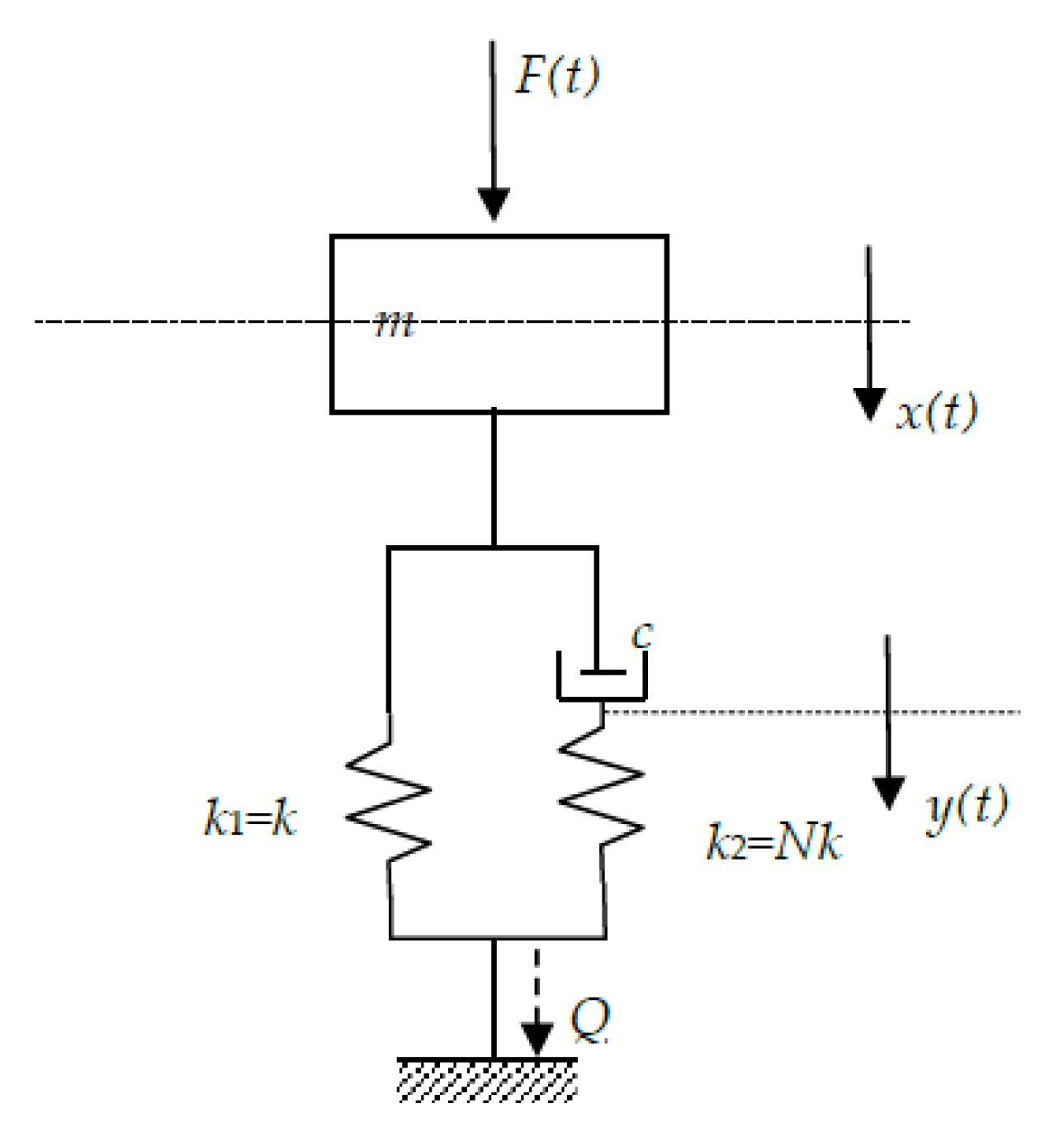
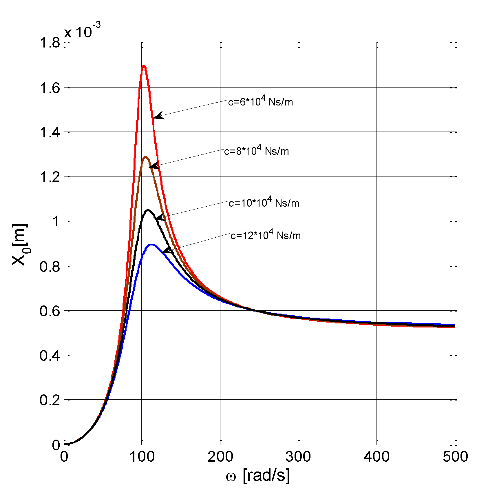
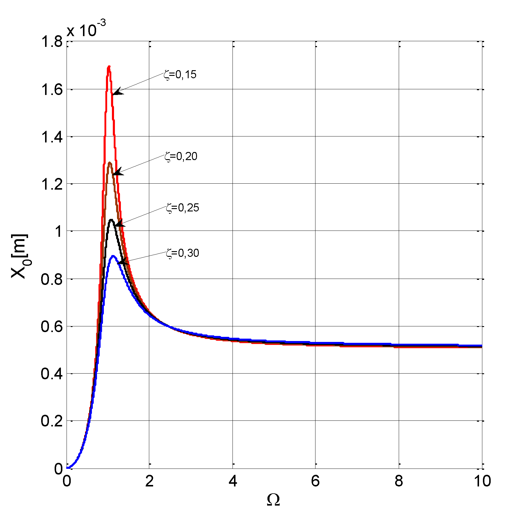
2. Dynamic Response with Respect to Displacements
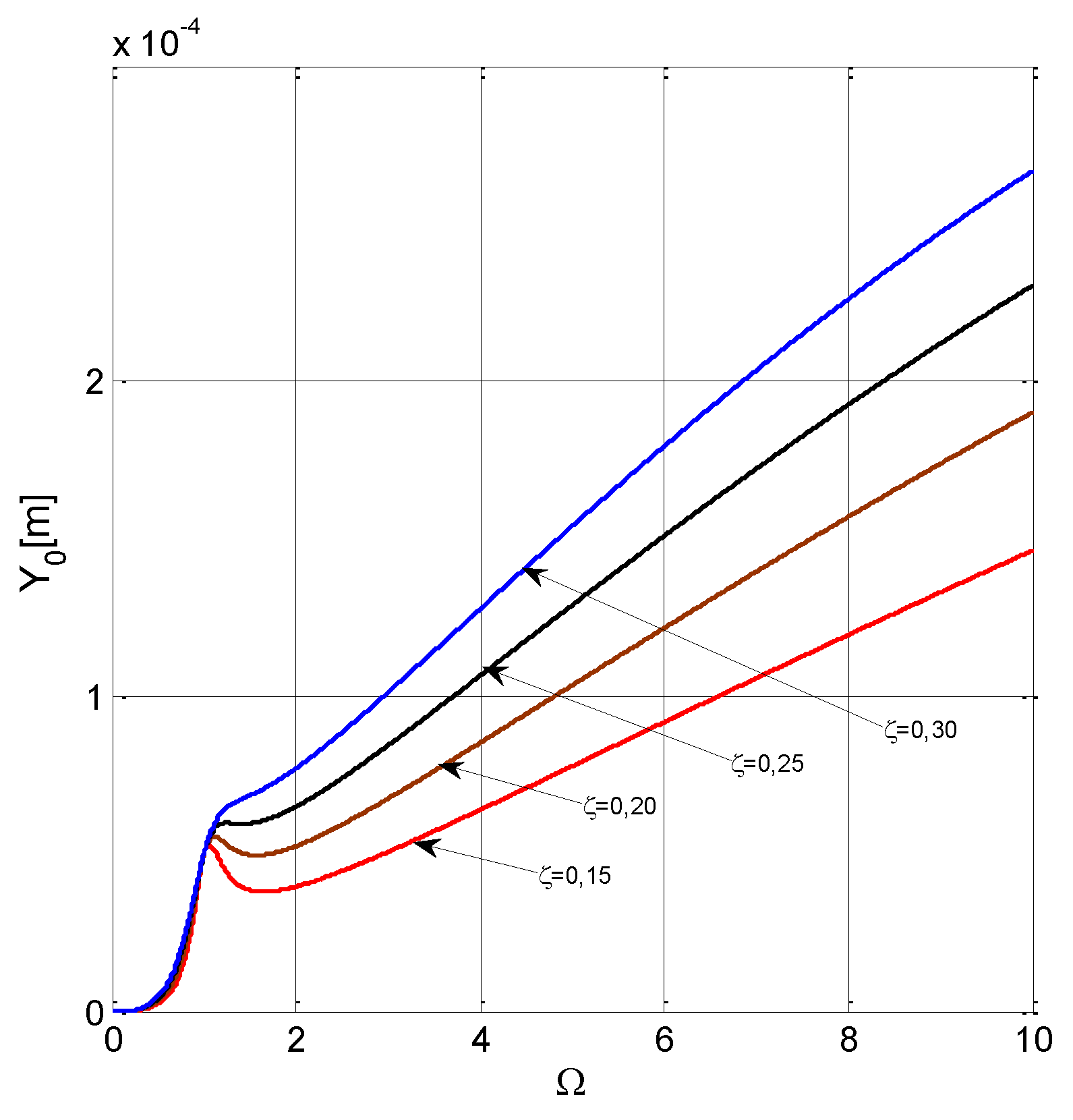
The viscoelastic materials, which can be modelled by a combination in parallel with the Hooke and Maxwell models, namely of the form E | ( E V ) , are characterized by a global rigidity reflecting both the elastic behaviour expressed by the rigidity coefficients k1, k2, and by the dissipative behaviour expressed by the dissipation coefficient c [4,5,6].
The dynamic model is presented in Figure 1, where F = F ( t ) = F 0 sin ω t , where either F 0 = m 0 r ω 2 , c is the linear viscous amortization proportional to the deformation speed of the viscous element, m is the mass, k1 = k rigidity of the Hooke elastic element, and k2 = kN is the rigidity of the elastic element in the structure of the Maxwell model, where N is a multiplication coefficient for rigidity k1 [7,8].
The parameter data for an experimental dynamic model are as follows: m = 4 × 10³ kg; m0r = 20 kgm; k = 108 N/m; N = 10; c = (7, 9, 11, 13) × 105 Ns/m; ζ = 0,15; 0,18; 0,22; 0,32; ω = 0...500 rad/s; Ω = 0...10 [1,7,8,9].
In complex wording, the movement differential equations are:
{ m x ˜ ¨ + k 1 x ˜ + k 2 y ˜ = F 0 e j ω t     c ( x ˜ ˙ y ˜ ˙ ) = k 2 y ˜
The response in instantaneous displacement is given by the relations:
x ˜ = X ˜ e j ω t ,   where   X ˜ = X 0 e j φ y ˜ = Y ˜ e j ω t ,   where   Y ˜ = Y 0 e j θ .
Introducing x ˜ , x ˜ ˙ , x ˜ ¨ , and y ˜ , y ˜ ˙ in Equation (1), we obtain the system in X ˜ and Y ˜ , as follows:
{ ( k 1 m ω 2 ) X ˜ + k 2 Y ˜ = F 0     j c ω X ˜ ( k 2 + j c ω ) Y ˜ = 0 ,
with the solutions:
X ˜ = F 0 k 2 + j c ω D ˜ ,
Y ˜ = F 0 j c ω D ˜ ,
where D ˜ = k 2 ( k 1 m ω 2 ) j c ω ( k 1 + k 2 m ω 2 ) .
If we introduce the following notations, α = k 2 , β = c ω , δ = k 2 ( k 1 m ω 2 ) , γ = c ω ( k 1 + k 2 m ω 2 ) , where D ˜ = δ j γ , Equations (4) and (5) may be rewritten:
X ˜ = F 0 α + j β δ + j γ = X 0 e j φ ,  
Y ˜ = F 0 j β δ + j γ = Y 0 e j θ .
For Equation (6), the complex form of X ˜ results as follows:
X ˜ = F 0 ( α + j β ) ( δ j γ ) ( δ + j γ ) ( δ + j γ ) , X ˜ = F 0 ( α δ + β γ ) + j ( β δ α γ ) δ 2 + γ 2 ,
therefore
| X ˜ | 2 = X 0 2 = F 0 2 ( α δ + β γ ) 2 + ( β δ α γ ) ( δ 2 + γ 2 ) 2
or
X 0 2 = F 0 2 α 2 + β 2 δ 2 + γ 2 ,
where we introduce α ,   β ,   δ ,   γ , and obtain:
X 0 = F 0 k 2 2 + c 2 ω 2 k 2 2 ( k 1 m ω 2 ) 2 + c 2 ω 2 ( k 1 + k 2 m ω 2 ) 2 .
We have from Equation (7):
Y ˜ = F 0 j β ( δ j γ ) ( δ + j γ ) ( δ j γ ) ,
or
Y ˜ = F 0 β γ + j β δ δ 2 + γ 2
therefore,
| Y ˜ | 2 = Y 0 2 = F 0 2 β 2 δ 2 + γ 2 ,
in which we replace the notations β ,   δ ,   γ , and obtain:
Y 0 = F 0 c ω k 2 2 ( k 1 m ω 2 ) 2 + c 2 ω 2 ( k 1 + k 2 m ω 2 ) 2 .
Phase terms φ and θ included in Equations (6) and (7) are determined as:
tg φ = β δ α γ α δ + β γ ,
or
tg φ = c ω k 2 2 k 2 2 ( k 1 m ω 2 ) + c 2 ω 2 ( k 1 + k 2 m ω 2 ) ,
and
tg θ = δ γ ,
therefore
tg θ = k 2 ( k 1 m ω 2 ) c ω ( k 1 + k 2 m ω 2 ) .
With relative sizes Ω = ω ω n ,   N = k 2 k , where k = k 1 = m ω n 2 ,   ζ = c 2 m ω n ,   c ω = ( 2 ζ Ω ) k , the amplitudes X 0 and Y 0 based on Equations (9) and (10) may be expressed as
X 0 = F 0 k N 2 + ( 2 ζ Ω ) 2 N 2 ( 1 Ω 2 ) 2 + ( 2 ζ Ω ) 2 ( N + 1 Ω 2 ) 2 ,
or
Y 0 = F 0 k 2 ζ Ω N 2 ( 1 Ω 2 ) 2 + ( 2 ζ Ω ) 2 ( N + 1 Ω 2 ) 2 .
Terms tg φ and tg θ , with relative sizes Ω , N , ζ , based on Equations (12) and (13), may be written as follows:
tg φ = 2 ζ Ω N 2 N 2 ( 1 Ω 2 ) + ( 2 ζ Ω ) 2 ( N + 1 Ω 2 ) ,
or
tg θ = ( 1 Ω 2 ) N ( 2 ζ Ω ) ( N + 1 Ω 2 ) .
The dynamic response to the excitation with force F ( t ) may be expressed by instantaneous displacements x = x ( t ) = X 0 sin ( ω t + φ ) and y = y ( t ) = Y 0 sin ( ω t + θ ) , where φ is the phase shift between x ( t ) and F ( t ) , and θ is the phase shift between y ( t ) and F ( t ) . In complex form, the dynamic response may be written as:
{ x ˜ = X ˜ 0 e j ( ω + φ ) y ˜ = Y ˜ 0 e j ( ω + θ ) ,
which yields
{ x = I m x ˜ = X 0 sin ( ω t + φ ) y = I m y ˜ = Y 0 sin ( ω t + θ )

Variation of Displacement Amplitudes X 0 and Y 0

(a) Case of natural parametersizes ω, c, k1, k2.
We introduce the amplitude of the excitation force in the Equations (9) and (10) as F 0 = m 0 r ω 2 .
For the continuous variation of the excitation pulsation ω and the discrete variation of the linear viscosity coefficient c, we have X 0 ( c ,   ω ) and Y 0 ( c ,   ω ) as [8,10,11]:
X 0 ( c , ω ) = m 0 r ω 2 N 2 k 2 + c 2 ω 2 N 2 k 2 ( k m ω 2 ) 2 + c 2 ω 2 ( k + N k m ω 2 ) 2 ,
Y 0 ( c , ω ) = m 0 r c ω 3 N 2 k 2 ( k m ω 2 ) 2 + c 2 ω 2 ( k + N k m ω 2 ) 2 ,
with representation in Figure 2 for X 0 ( c , ω ) and in Figure 3 for Y 0 ( c , ω ) , where X 0 , Y 0 is in m, ω in rad/s, c in Ns/m.
(b) Case with relative sizes Ω , ζ , N :
X 0 ( ζ , Ω ) = m 0 r m Ω 2 N 2 + ( 2 ζ Ω ) 2 N 2 ( 1 Ω 2 ) 2 + ( 2 ζ Ω ) 2 ( N + 1 Ω 2 ) 2 ,
Y 0 ( ζ , Ω ) = m 0 r m Ω 2 2 ζ Ω N 2 ( 1 Ω 2 ) 2 + ( 2 ζ Ω ) 2 ( N + 1 Ω 2 ) 2 ,
with representation in Figure 4 for X 0 ( ζ , Ω ) and in Figure 5 for Y 0 ( ζ , Ω ) for the force F 0 = m 0 r m k Ω 2 .

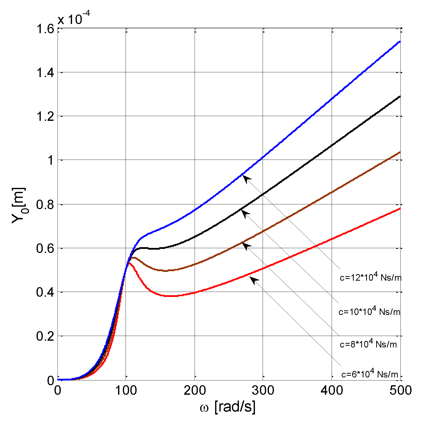
3. Transmitted Dynamic Force

The force Q ˜ = Q ˜ ( t ) transmitted to the fixed base represents the effect of the connection ( E | E V ) in a dynamic regime, which can be formulated as [12,13]:
Q ˜ = Q ˜ ( t ) = k x ˜ + N k y ˜ ,
where k = k 1 ,     and   N k   = k 2 .
Introducing x ˜ and y ˜ as
x ˜ = X ˜ e j ω t = F 0 N k + j c ω D ˜ , y ˜ = Y ˜ e j ω t = F 0 j c ω D ˜ ,
in Equation (24), we obtain
Q ˜ = F 0 D ˜ [ N k 2 + j c ω k ( 1 N ) ] .
We introduce D ˜ = N k ( k m ω 2 ) +   j c ω ( k + N k m ω 2 ) in Equation (25) and obtain
Q ˜ = F 0 N k 2 + j c ω k ( 1 N ) N k ( k m ω 2 ) +   j c ω ( k + N k m ω 2 ) ,
By making q 1 = N k 2 ;   q 2 = c ω k ( 1 + N ) ;   q 3 = N k ( k m ω 2 ) ;   q 4 = c ω ( k + N k m ω 2 ) , Equation (26) becomes
Q ˜ = F 0 q 1 + j q 2 q 3 + j q 4 ,
from which Q 0 2 becomes
| Q ˜ | 2 = Q 0 2 = F 0 2 q 1 2 + q 2 2 q 3 2 + q 4 2
and the amplitude of the transmitted force Q 0 is
Q 0 = F 0 q 1 2 + q 2 2 q 3 2 + q 4 2   ,
Replacing q 1 ; q 2 ; q 3 ; q 4 with prior notations, we obtain Q 0 in natural sizes, as follows:
Q 0 ( c , ω ) = F 0 N 2 k 4 + c 2 ω 2 k 2 ( 1 N ) 2 N 2 k 2 ( k m ω 2 ) 2 +   c 2 ω 2 ( k + N k m ω 2 ) 2   ,
In the relative parameters Ω , ζ , and N, Equation (28) may be written as
Q 0 ( ζ , Ω ) = F 0 N 2 + ( 2 ζ Ω ) 2 ( 1 N ) 2 N 2 ( 1 Ω 2 ) 2 + ( 2 ζ Ω ) 2 ( N + 1 Ω 2 ) 2 ,

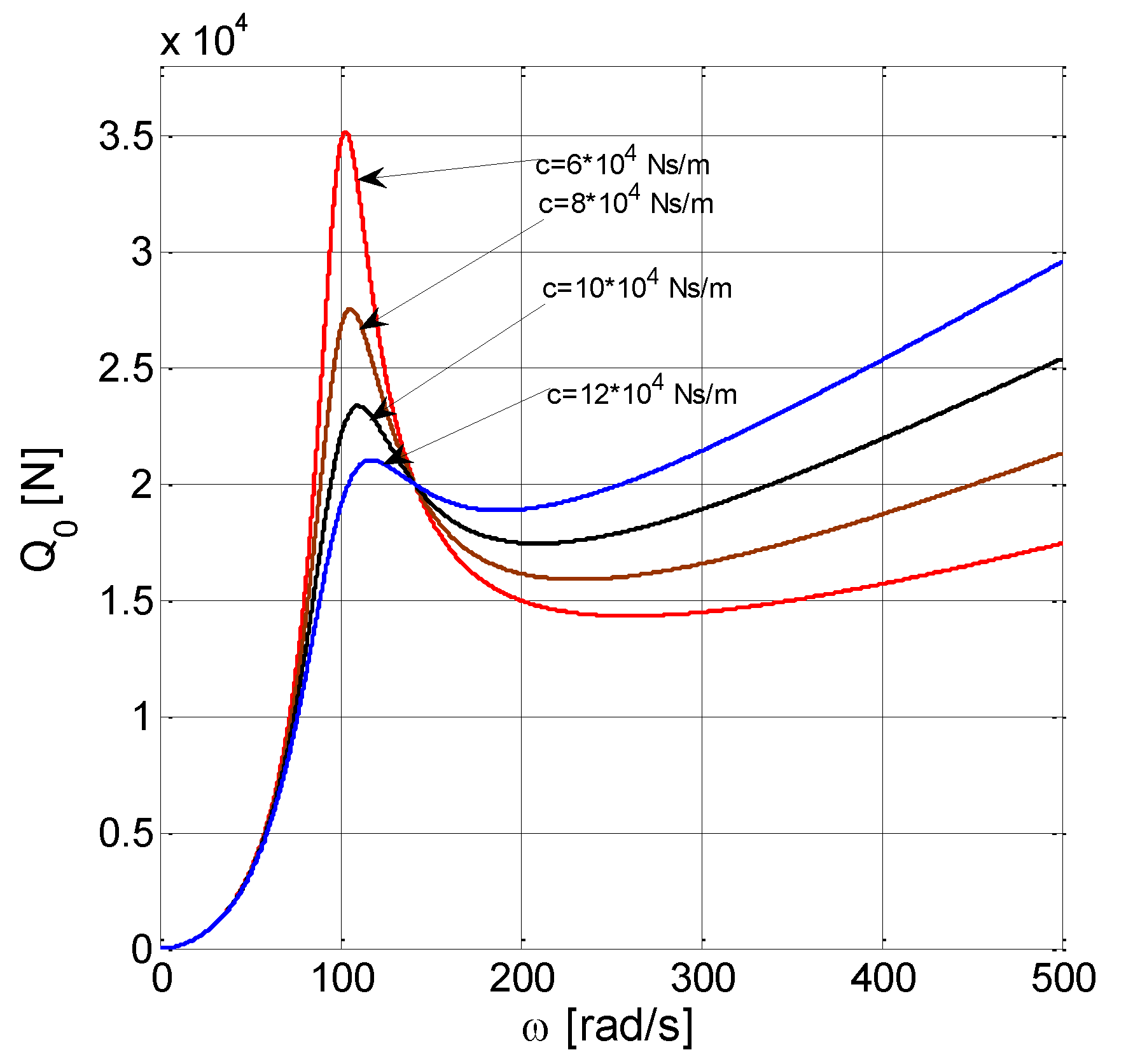
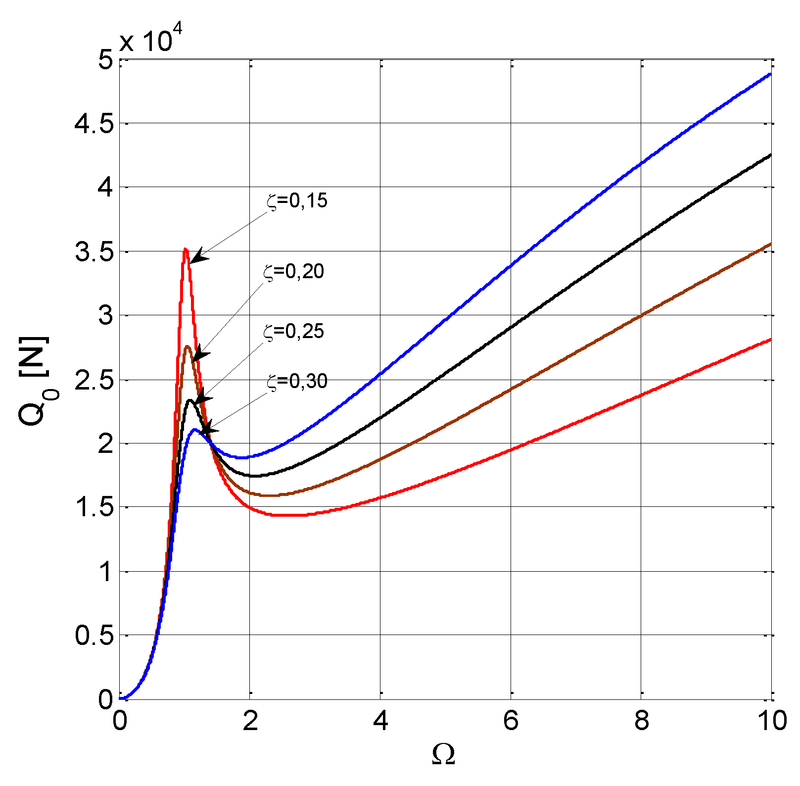
Variation of transmitted force amplitude Q 0

(a) Case of natural sizes
Q 0 ( c , ω ) = m 0 r ω 2 · R ( c , ω )
where R ( c , ω ) is given by the relation
R ( c , ω ) = N 2 k 4 + c 2 ω 2 k 2 ( 1 N ) 2 N 2 k 2 ( k m ω 2 ) 2 +   c 2 ω 2 ( k + N k m ω 2 ) 2  
(b) Case of relative sizes
  Q 0 ( ζ , Ω ) = m 0 r m k Ω 2 · R ( ζ , Ω )
where R ( ζ , Ω ) is given by the relation
R ( ζ , Ω ) = N 2 + ( 2 ζ Ω ) 2 ( 1 N ) 2 N 2 ( 1 Ω 2 ) 2 + ( 2 ζ Ω ) 2 ( N + 1 Ω 2 ) 2
The force Q 0 ( c , ω ) is presented in Figure 6, while Figure 7 shows a representation of force Q 0 ( ζ , Ω ) at force F 0 = m 0 r ω 2 , which is, respectively, F 0 = m 0 r m k Ω 2 .

4. The Capacity of Dynamic Insulation

The force transmissibility is given by the relation T = Q 0 F 0 and may be respective to the natural or relative sizes.
In this case, based on Equations (28)–(31), we have
T ( c , ω ) = Q 0 ( c , ω ) F 0 = R ( c , ω )
or
T ( ζ , Ω ) = Q 0 ( ζ , Ω ) F 0 = R ( ζ , Ω ) .

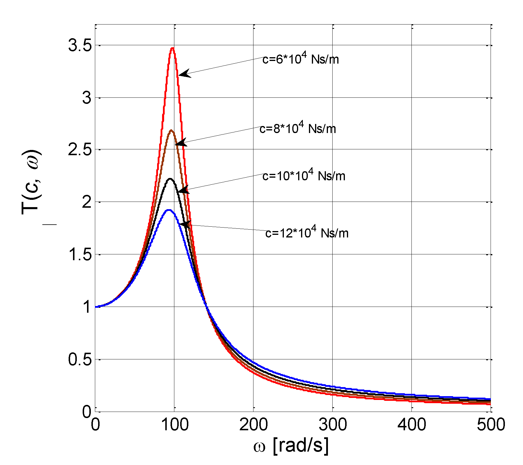
Variation of Force Transmissibility

For transmissibility T ( c , ω ) and T ( ζ , Ω ) , considering F 0 = m 0 r ω 2 and F 0 = m 0 r m k Ω 2 , respectively, we have
T ( c , ω ) = Q 0 ( c , ω ) m 0 r ω 2 = R ( c , ω )
or
T ( ζ , Ω ) = Q 0 ( ζ , Ω ) m 0 r k · m Ω 2 = R ( ζ , Ω ) ,
which are represented in Figure 8.

5. Amplitude of Instantaneous Deformation for a Linearly Viscous Buffer.

For the linearly viscous buffer with c characteristics, the instantaneous deformation may be assessed by two methods [6,9,10,11]:
MethodI
The instantaneous deformation z ˜ is given by the relation
z ˜ = x ˜ + y ˜
where we introduce x ˜ and y ˜ as follows:
x ˜ = X ˜ e j ω t ;   y ˜ = Y ˜ e j ω t z ˜ = F 0 ( α δ + β γ ) δ 2 + γ 2 j β δ α γ δ 2 + γ 2 + F 0 β γ + j β δ δ 2 + γ 2 z ˜ = F 0 [ α δ j α γ δ 2 + γ 2 ]
thus
Z 0 2 = F 0 2 α 2 δ 2 + α 2 γ 2 ( δ 2 + γ 2 ) 2 = α 2 F 0 2 1 δ 2 + γ 2
or
Z 0 = α F 0 δ 2 + γ 2 .
MethodII
From c z ˙ ˜ = k 2 y ˜ or c z ˙ ˜ = k 2 F 0 β γ + j β δ δ 2 + γ 2 e j ω t , and recalling that k 2 = α and β = c ω , it follows that
z ˙ ˜ = d z ˜ d t = α F 0 c · β γ + j β δ δ 2 + γ 2 e j ω t ,
so
z ˜ = α β F 0 c · γ + j δ δ 2 + γ 2 e j ω t d t ,
or
z ˜ = α F 0 j · γ + j δ δ 2 + γ 2 .
The expression z ˜ may be established as a complex number. Therefore,
z ˜ = α F 0 δ 2 + γ 2 [ δ j γ ] = Z 0 e i φ 0 ,
so we have
α 2 F 0 2 ( δ 2 + γ 2 ) 2 [ δ 2 + γ 2 ] = Z 0 2
or Z 0 = α F 0 δ 2 + γ 2 , which is identical to that from method I, respective to Equation (36).
Returning to natural size, we obtain
Z 0 ( c , ω ) = N k F 0 N 2 k 2 ( k m ω 2 ) 2 +   c 2 ω 2 ( k + N k m ω 2 ) 2 ,
and returning to relative sizes, we have
Z 0 ( ζ , Ω ) = F 0 k N N 2 ( 1 Ω 2 ) 2 + ( 2 ζ Ω ) 2 ( N + 1 Ω 2 ) 2 .

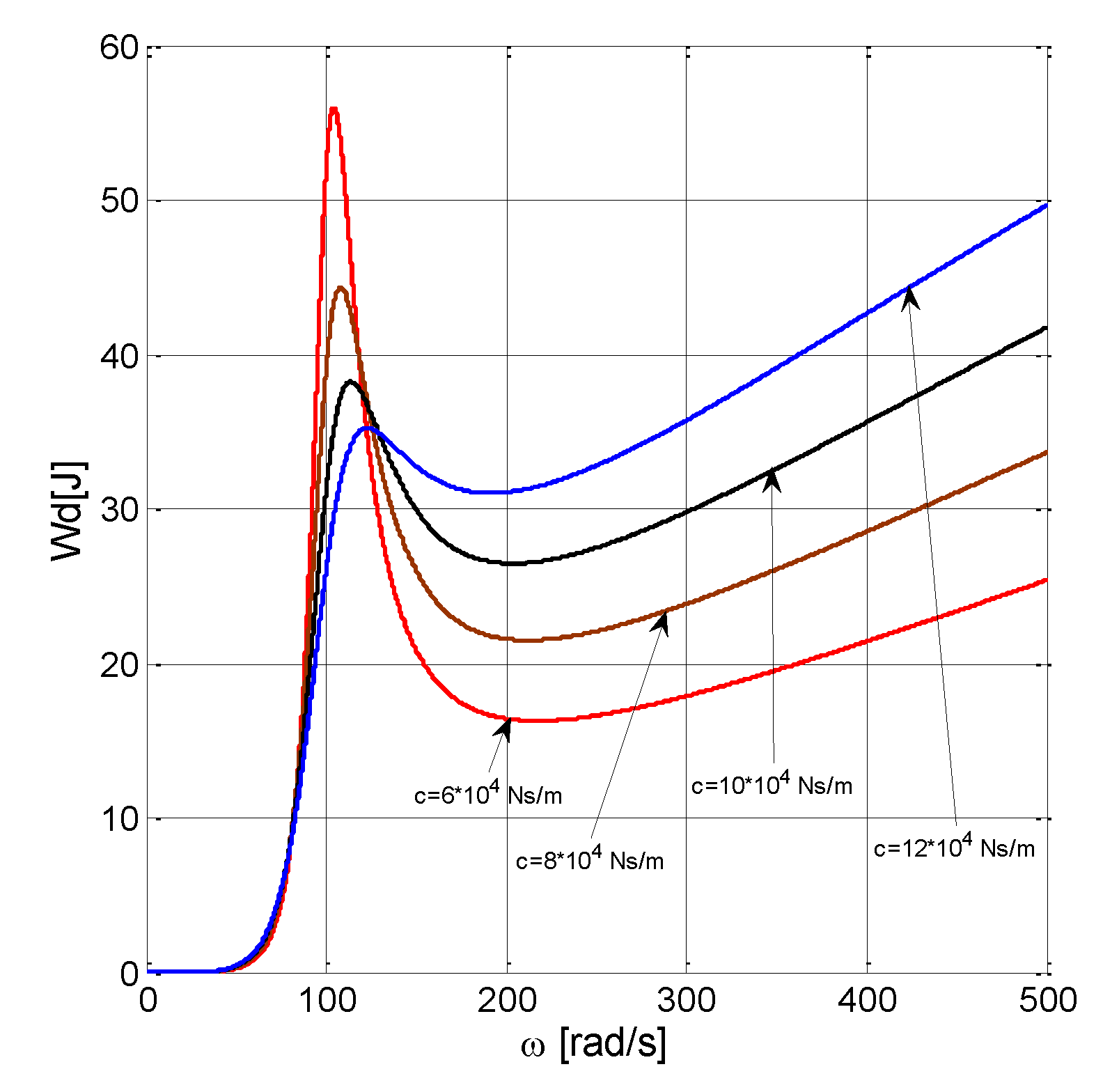
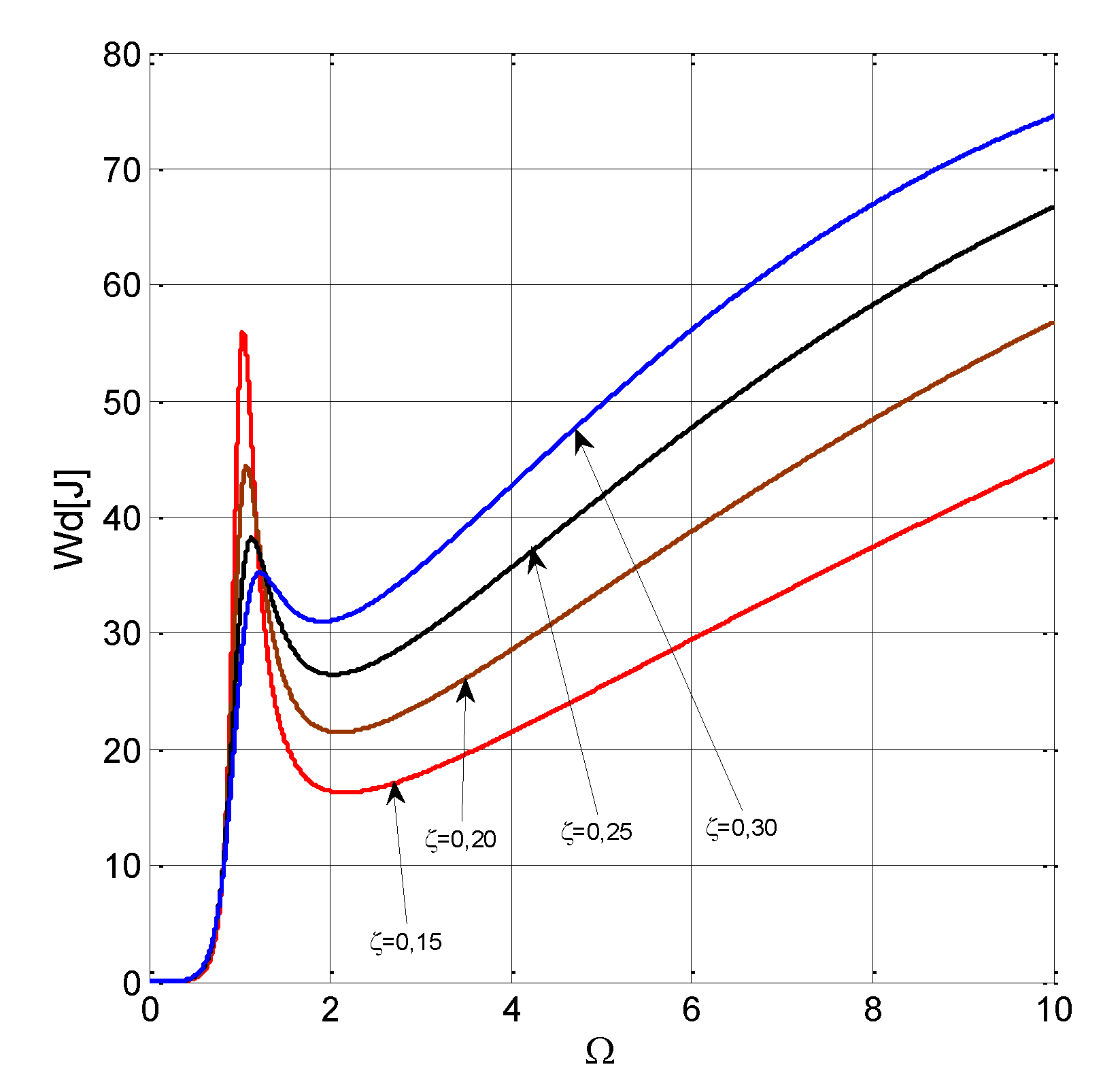
6. Dissipated Energy

In the Zener model, the energy dissipated per cycle is expressed as
W d = π c ω Z 0 2 .
Replacing Z 0 from Equation (41) and (42), we determine the dissipated energy per cycle as
W d ( c , ω ) = π ( m 0 r ) 2 c ω 5 N 2 k 2 N 2 k 2 ( k m ω 2 ) 2 +   c 2 ω 2 ( k + N k m ω 2 ) 2
or
W d ( ζ ,   Ω ) = π ( m 0 r m ) 2 k ( 2 ζ Ω 5 ) N 2 N 2 ( 1 Ω 2 ) 2 + ( 2 ζ Ω ) 2 ( N + 1 Ω 2 ) 2
with the graphic representations in Figure 9 and Figure 10.

7. Conclusions

The Zener linear viscoelastic model may be used to study the dynamic behaviour of materials, systems, and structures that are technologically manufactured both to assure predictable values for the dynamic forces transmitted to the base and to evaluate the dissipated energy. Based on some anti-vibrating devices assembled to follow the Zener linear model, solutions for the dynamic insulation of the industrial vibrations for dynamic equipment in a technological flow at working frequencies ranging from 20 Hz to 50 Hz have been studied and established.
In addition, Zener type dynamic behaviors were identified when compacting process is made by vibrating rolls and for certain stratifications of the road structures [1,2,3,7,8].
Numerical analysis and experimental data allowed for the adjustment of a Zener rheological model, with mass and harmonic excitation using inertial rotating force.
(a)
The analytical model and parametric curves lead to the following conclusions:
(b)
The X0 and Y0 amplitudes define the largest displacements of the mass m, and, respectively, of the elastic component k2 = kN, which is useful in the evaluation of the technological parameters [4,5,7];
(c)
The parametric curves of amplitudes X0 and Y0 show distributions depending on on the ante-resonance, resonance, and post-resonance dynamic regimes [3,7,14,15];
The dynamic area of interest for the stable behaviour of the technological vibrations is specific to the post-resonance field [1,7,15];
Thus, for significantly high values of the excitation pulsations, in conditions of predictable amortization, the X0 amplitude presents a stable layer at low variations of the excitation pulsation, suggesting that Y0 continuously increased with ω.
(d)
The maximal dynamic transmitted force Q0 in the post-resonance field for ω >> ωn or Ω >> 1 shows the stable values set by the size of the viscous amortization.
(e)
Transmissibility decreases at high values of the excitation pulsation once a discrete value is set for amortization.
(f)
The dissipated energy increases in the post-resonance stage along with the excitation frequency and amortization level [1,8,12,13].
Consequently, based on the physical–mechanical parameters specific to the Zener rheological model for viscoelastic materials, systems, and structures, assessments can be performed on the parameter sizes of the dynamic answer and behaviour in the harmonic excitation regime with harmonic rotation forces.
The input numerical values presented for the case study show that for a composition of land where predominant material is clay 60%, sand (10–15%), mineral aggregates (20%), stabilizer (1%), water (10–18%), the Zener model, according to the response values, reflects with high fidelity the rheological behavior at the excitation pulse ω = (250...320) rad/s or Ω = 1.5 ÷ 2.5.
For the excitation pulse interval of interest mentioned, the technological effect, expressed as good compacting, is given by the parametric values for the amplitude of the forced vibrations X0 = 0,005 m, the force transmitted to the field Q0 = (1,5 ÷ 2,5) × 103 kN, and the dissipated energy Wd = (10 ÷ 25) kJ.

Author Contributions

P.B. designed the rheological model based on the experimental data and formulated the dynamic equations and established calculation formulas for the dissipated energy; C.D. provided the experimental data in the form of input parameters for the vibratory compactor dynamic model and for the viscous-linear characteristics of the compacted earth. She also set the computation formulas for field strength correlated with dissipated energy and degree of compaction.

Funding

This research received no external funding.

Conflicts of Interest

The authors declare no conflict of interest.

References

  1. Bratu, P.; Stuparu, A.; Leopa, A.; Popa, S. The dynamic analyse of a construction with the base insulation consisting in anti-seismic devices modeled as a Hooke-Voigt-Kelvin linear rheological system. Acta Tech. Napoc. Ser. Appl. Math. Eng. 2018, 60, 465–472. [Google Scholar]
  2. Bratu, P.; Stuparu, A.; Popa, S.; Iacob, N.; Voicu, O.; Iacob, N.; Spanu, G. The dynamic isolation performances analysis of the vibrating equipment with elastic links to a fixed base. Acta Tech. Napoc. Ser. Appl. Math. Eng. 2018, 61, 23–28. [Google Scholar]
  3. Dobrescu, C.F. Highlighting the Change of the Dynamic Response to Discrete Variation of Soil Stiffness in the Process of Dynamic Compaction with Roller Compactors Based on Linear Rheological Modeling. Appl. Mech. Mater. 2015, 801, 242–248. [Google Scholar] [CrossRef]
  4. Adam, D.; Kopf, F. Theoretical Analysis of Dynamically Loaded Soils, European Workshop: Compaction of Soils and Granular Materials; ETC11 of ISSMGE: Paris, France, 2000. [Google Scholar]
  5. Bejan, S. Analiza Performanței Procesului de Compactare Dinamică Prin Vibrații Pentru Structuri Rutiere. Ph.D. Thesis, “Dunarea de Jos” University of Galati, Galați, Romania, 2015. [Google Scholar]
  6. Bratu, P. The behavior of nonlinear viscoelastic systems subjected to harmonic dynamic excitation. In Proceedings of the 9th International Congress on Sound and Vibration, University of Central Florida, Orlando, FL, USA, 8–11 July 2002. [Google Scholar]
  7. Bratu, P.; Debeleac, C. The analysis of vibratory roller motion. In Proceedings of the VII International Triennial Conference Heavy Machinery–HM 2011, Session Earth-moving and transportation machinery, Vrnjačka Banja, Serbia, 29 June–2 July 2011; pp. 23–26, ISBN 978-86-82631-58-3. [Google Scholar]
  8. Bratu, P.; Stuparu, A.; Popa, S.; Iacob, N.; Voicu, O. The assessment of the dynamic response to seismic excitation for constructions equipped with base isolation systems according to the Newton-Voigt-Kelvin model. Acta Tech. Napoc. Ser. Appl. Math. Eng. 2017, 60, 459–464. [Google Scholar]
  9. Bratu, P. Dynamic response of nonlinear systems under stationary harmonic excitation, Non-linear acoustics and vibration. In Proceedings of the 11th International Congress on Sound and Vibration, St. Petersburg, Russia, 5–8 July 2004; pp. 2767–2770. [Google Scholar]
  10. Dobrescu, C.F.; Brăguţă, E. Optimization of Vibro-Compaction Technological Process Considering Rheological Properties. In Springer Proceedings in Physics, Proceedings of the 14th AVMS Conference, Timisoara, Romania, 25–26 May 2017; Herisanu, N., Marinca, V., Eds.; Springer: Berlin/Heidelberg, Germany, 2017; pp. 287–293. [Google Scholar] [CrossRef]
  11. Leopa, A.; Debeleac, C.; Năstac, S. Simulation of Vibration Effects on Ground Produced by Technological Equipments. In Proceedings of the 12th International Multidisciplinary Scientific GeoConference and EXPO-Modern Management of Mine Producing, Geology and Environmental Protection, SGEM 2012, Albena, Bulgaria, 17–23 June 2012; Volume 5, pp. 743–750. [Google Scholar]
  12. Morariu-Gligor, R.M.; Crisan, A.V.; Şerdean, F.M. Optimal design of an one-way plate compactor. Acta Tech. Napoc. Ser. Appl. Math. Mech Eng. 2017, 60, 557–564. [Google Scholar]
  13. Pințoi, R.; Bordos, R.; Braguța, E. Vibration Effects in the Process of Dynamic Compaction of Fresh Concrete and Stabilized Earth. J. Vib. Eng. Technol. 2017, 5, 247–254. [Google Scholar]
  14. Mooney, M.A.; Rinehart, R.V. Field Monitoring of Roller Vibration During Compaction of Subgrade Soil. J. Geotech. Geoenviron. Eng. ASCE 2007, 133, 257–265. [Google Scholar] [CrossRef]
  15. Mooney, M.A.; Rinehart, R.V. In-Situ Soil Response to Vibratory Loading and Its Relationship to Roller-Measured Soil Stiffness. J. Geotech. Geoenviron. Eng. ASCE 2009, 135, 1022–1031. [Google Scholar] [CrossRef]
Figure 1. Zener linear model E | ( E V ) with harmonically excited mass.
Symmetry 11 01050 g001
Figure 2. Plots of   X 0 ( c , ω ) for continuously varying ω and discrete values of c.
Symmetry 11 01050 g002
Figure 3. Plots of Y 0 ( c , ω ) for continuously varying ω and discrete values of c.
Symmetry 11 01050 g003
Figure 4. Plots of   X 0 ( ζ , Ω ) for continuously varying Ω and discrete values of ζ.
Symmetry 11 01050 g004
Figure 5. Plots of   Y 0 ( ζ , Ω ) for continuously varying Ω and discrete values of ζ.
Symmetry 11 01050 g005
Figure 6. Plots of transmitted force amplitude Q 0 ( c , ω ) for continuously varying ω and discrete values of c. The excitation force amplitude F0 is expressed as F 0 = m 0 r ω 2 .
Symmetry 11 01050 g006
Figure 7. Plots of transmitted force amplitude Q 0 ( ζ , Ω ) for continuously varying Ω and discrete values of ζ. Excitation force amplitude F0 is expressed as F 0 = m 0 r m k Ω 2 .
Symmetry 11 01050 g007
Figure 8. Plots of force transmissibility T ( c , ω ) for continuously varying ω and discrete values of c. Excitation force amplitude Fo is expressed as F 0 = m 0 r ω 2 .
Symmetry 11 01050 g008
Figure 9. Plots of the dissipated energy per unit cycle W d ( c , ω ) for continuously varying ω and discrete values of c. The excitation force amplitude F0 is expressed as F 0 = m 0 r ω 2 .
Symmetry 11 01050 g009
Figure 10. The plots of the dissipated energy per unit cycle W d ( ζ , Ω ) for continuously varying Ω and discrete values of ζ. The excitation force amplitude F0 is expressed as   F 0 = m 0 r m k Ω 2 .
Symmetry 11 01050 g010

