Retardant Effects of Collapsing Dynamics of a Laser-Induced Cavitation Bubble Near a Solid Wall

Abstract

In the present paper, the dynamic behavior of cavitation bubbles near a wall is experimentally investigated with a focus on the retardant effects of the wall on the collapsing dynamics of the bubble. In the present experiments, a cavitation bubble is generated by a focused laser beam with its behavior recorded through high-speed photography. During the data analysis, the influences of non-dimensional bubble–wall distance on the bubble collapsing dynamics are qualitatively and quantitatively investigated in terms of the interface evolution, the velocities of the poles, and the movement of the bubble centroid. Our results reveal that the presence of the wall could significantly affect the collapsing characteristics, leading to a dramatic difference between the moving velocities of interfaces near and away from the wall. With the decrease of the bubble–wall distance, the effects will be gradually strengthened with a rapid movement of the bubble centroid during the final collapse. Finally, a physical interpretation of the phenomenon is given based on the bubble theory, together with a rough estimation of the induced water hammer pressure by the bubble collapse.

1. Introduction

Cavitation bubble dynamics near a solid plane wall is of great importance for many essential industrial applications. For example, in hydro-turbines [1,2] or pumps [3], the bubble shows violent oscillations with a prominent interface speed, generating strong shock waves during its final collapse. Furthermore, a toroidal shape bubble will also be seen with a tiny-scale micro-jet towards the wall. Hence, hydraulic facilities are greatly threatened by the presence of cavitation bubbles. On the contrary, the above damaging potential of a cavitation bubble could be also employed for various kinds of applications, such as cleaning of dirt [4,5]. In order to protect a surface from cavitation damage or enhance the cavitation-induced physical benefits (e.g., effective cleaning), the detailed physical process of the cavitation dynamics during the whole event should be fully explored.

Bubble–wall interactions have been intensively investigated by numerous researchers with the following categories: solid wall (e.g., plane [6,7,8,9,10,11], concave [12], convex [12]), elastic wall (e.g., resilient structure [13], membrane [14], biological tissue [15]), composite materials, particles [16,17,18], gaps [19], two parallel walls [20], free surfaces [21,22], and non-Newtonian fluids [23,24,25,26], together with the axisymmetric body [27]. For reviews of the present topic, Blake and Gibson [28], Lauterborn [29], Section 3 of Brennen [30] and Wang et al. [31] are suggested. Here, our attention is mainly focused on the cavitation collapsing dynamics near a plane solid wall.

According to the distance between the bubble and the wall, the previous findings on the cavitation near a plane solid wall could be summarized as follows.

For a large distance, the bubble nearly retains its spherically symmetrical shape during its dynamic oscillations. Hence, a radial fluid flow will be generated by the volumetric oscillations of the bubbles. During the whole process, because of the significant distance from the wall, the bubble has no direct contact with the wall.

For a medium distance, the bubble shows some non-spherical oscillations with observable movement towards the wall. The fluid field around the bubble becomes complex with vortex generations. Depending on the exact distance, the bubble may contact the wall (usually during its second cycle).

For a short distance, the bubble shows great interface deformations in different directions. During its final collapse, a distinguished toroidal bubble is formed with a jet inside the bubble [32]. When the distance is extremely short, the formation and the properties of the jet alter strongly.

In the literature, bubble–wall interactions have been intensively investigated by many researchers using in-house code (e.g., boundary integral method [33,34,35,36]) or open source code (e.g., OpenFOAM [37,38]). Specifically, Lee et al. [33] incorporated energy loss through a discontinuous jump function in the potential energy during the bubble status with minimum volume. Wang [34] employed a weakly compressible theory for the predictions of the damped oscillations with a vortex ring model for the predictions of the toroidal bubble. The bubble oscillations within several cycles were successfully predicted with the energy loss through shock wave generations. Han et al. [36] investigated the weak and strong bubble–bubble interactions near a rigid boundary with a detailed discussion on the jet characteristics. Koch et al. [37] proposed new code based on the finite volume and the volume of fluid methods for the bubble phenomenon predictions using OpenFOAM. Lechner et al. [38] further employed the aforementioned code for the simulations of a bubble very close to the boundary and found that a thin and fast jet could be demonstrated.

In the present paper, the retardant effect of a laser-induced cavitation bubble near a solid plane wall is experimentally investigated by employing a high-speed camera. Here, a brief description of the retardant effect will be given with the aid of Figure 1. Figure 1 shows a brief description of the bubble–wall system with the definitions of several important control parameters in the present experiment. In the figure, the gray sphere represents the cavitation bubble, and the gray rectangle represents the rigid wall. The point O represents the origin of the coordinate system and the point M represents the inception point of the cavitation. The points A and B represent the two poles of the cavitation bubble. The positive velocity direction of pole A and pole B is pointing toward the wall. During the collapse stage of the cavitation bubbles near the wall, different partitions of the bubble interface show dramatically different movements. For example, pole B shown in Figure 1 close to the wall moves much slower than pole A away from the wall. This difference will significantly alter the bubble behavior in the later stage. In the literature, the details of the aforementioned retardant effect have not been clearly investigated, especially in a quantitative way. Here, qualitative and quantitative studies of the retardant effects of the wall presence on the collapsing shape of the bubble (e.g., different collapsing speed of the two partitions with one near the wall and the other away from the wall) are both undertaken in detail.

During our experiments, a series of bubble–wall interaction cases are investigated in terms of the standing-off distance. For the qualitative study, high-speed photographs are employed to illustrate the characteristics of the bubble–wall interactions. For the quantitative study, the collapsing velocities of two bubble poles are given together with the bubble centroid movement. For the convenience of readers, the topics of the following sections are organized as follows. Section 2 describes the experimental setup together with the definitions of key parameters and several non-dimensional parameters involved in the present paper. Section 3 qualitatively illustrates the dynamic behaviors of the cavitation bubble with different bubble–wall distances during their collapsing stages. Section 4 quantitatively discusses the influences of the bubble–wall distance on the interface velocities of the cavitation bubble with the aid of several typical examples. Section 5 quantitatively investigates the evolution of the bubble interfaces and the movement of the cavitation bubble centroid during its collapsing stage. Section 6 further explains the physical mechanisms related to the observed phenomenon. Section 7 gives a brief summary of the conclusive points.

2. Experimental Setup

The present experimental facilities consists of a laser-based bubble generating system. For a very detailed description of the whole system (e.g., the cavitation generation and lighting systems), readers can refer to our recent previous work [16]. In the present paper, the same experimental facilities were employed for studying bubble–wall interactions. Briefly speaking, the present system employed a focused Nd:YAG laser beam to convert laser energy into a bubble explosion in water. Meanwhile, a high-speed camera was employed to record the whole bubble events for each parameter setup. For the principles of high-speed imaging, readers are referred to Thoroddsen et al. [39]. One of the advantages of the present bubble system is stability in terms of accurate control of the bubble size and repetition of the phenomenon. A brief description of the experimental procedures is as follows:

• Check the connections between different systems, e.g., signal transmission.
• Place the solid wall in a suitable place through the 3D platform.
• Generate bubbles using focused laser. Meanwhile, trigger the camera and the flashing lights. The delays between the three elements could be adjusted for different purposes.
• Save the data and check its quality.
• Repeat the same parameter setup several times for repeatability.
• Try another distance between the bubble and wall or different bubble sizes controlled by the laser energy.

As shown in Figure 1, several essential parameters involved are defined clearly. For the convenience of the following discussions, a non-dimensional parameter λ reflecting the bubble standing-off distance is defined as:

$$\lambda =\frac{L}{R_{\max }}$$

(1)

where R_max is the equivalent maximum radius of the cavitation bubble during its dynamic oscillations, also corresponding to the maximum bubble volume; L is the distance between the inception point of the bubble and the surface of the solid wall. In order to analyze the data, the Phantom Camera Control (PCC) application was employed for the accurate measurement of R_max and L. In the present paper, a series of experiments with different R_max (7 values) and L (13 values) were conducted with the variations of λ within [0.2, 3.0].

The images shown in the present paper were shot by a high-speed camera (Phantom V1212) at 240,000 frames per second (fps). For further discussion, in order to describe the retardant effects of the wall on the cavitation bubble collapse, the bottom-most point (defined as pole A) and the upper-most point (defined as pole B) are employed. Furthermore, $V_A$ and $V_B$ represent the velocity of the poles A and B during the collapsing stage of the cavitation bubble with:

$$\Delta V=\left|V_B|-|V_A\right|.$$

(2)

For the convenience of the following descriptions, a non-dimensional time ($\tau$) is defined as follows:

$$\tau =\frac{t-t_{R_{\max }}}{T_c}$$

(3)

where $t$ represents the time from the generation of the cavitation bubble to the current moment; $t_{R_{\max }}$ represents the time from the generation of the cavitation bubble to the moment when it reaches its maximum volume; $T_c$ represents the overall time of the collapsing stage (from the moment when bubble reaches its maximum volume to the final collapse) of the cavitation bubble (see subplots 9–14 of Figure 2). Hence, for $\tau =0$, the volume of the cavitation bubble reaches its maximum at the current moment; for $\tau =1$, the cavitation bubble is at the moment of its final collapse. Furthermore, the critical time above which $\Delta V$ reaches 5 m/s, is further defined as ${\tau }_{crit}$.

In order to discuss the movement of the centroid of the cavitation bubble, the moving distance ($\Delta D$) of the bubble centroid during the collapsing stage is defined as follows:

$$\Delta D=D_0-D$$

(4)

where $D$ represents the instantaneous distance between the wall and the centroid of the cavitation bubble; and $D_0$ represents the distance between the wall and the centroid of the cavitation bubble at the moment of time $\tau =0$ (or $t=t_{R_{\max }}$).

3. Qualitative Descriptions of the Cavitation Bubble Dynamic Behavior Near the Wall

In this section, the influences of the standing-off distance on the cavitation bubble dynamic behavior near the wall are qualitatively assessed. In Section 3.1, a general case of the cavitation bubble–wall interaction is illustrated and the dynamic behavior of the cavitation bubble is divided into several stages, from the cavitation inception to its collapse. In Section 3.2, influences of the standing-off distance on the retardant effects during the bubble collapse stages are qualitatively assessed in terms of three typical examples.

3.1. Typical Examples of the Collapse of a Cavitation Bubble Near a Wall

Figure 2 shows the photos of the dynamic behavior of a cavitation bubble collapsing near a wall. In order to compare the movement of the bubble interface (especially the left-most and right-most positions), all the subplots have been rotated 90 degrees clockwise, with the direction of gravity to the left. For the convenience of the reader, only the essential middle parts of the recorded photos are retained. In the figure, in order to describe the behavior of the cavitation bubble, 21 subplots are selected and arranged with a chronological order (with the inter-frame time intervals being 12.5 µs). As shown in subplot 7, the bubble reaches its maximum volume (or maximum bubble radius R_max) with the left-most position at the point A and the right-most position at the point B, respectively (denoted poles A and B for short). In order to show the movement of the bubble interface more clearly, two vertical dashed lines are marked in the figure with the yellow and the blue lines passing the points A and B, respectively.

In Figure 2, the whole dynamic behavior of the cavitation bubble near the wall can be divided into several stages as follows (also marked in the figure). Firstly, the cavitation bubble is initially generated by the focused laser beams above the wall (subplot 1 of Figure 2, denoted “cavitation inception”). Then, with the input of the laser energy, the bubble immediately steps into the stage of growth (subplot 2–7 of Figure 2) with the bubble radius gradually expanding. During the growth stage, the bubble shape is basically spherical. Then, the cavitation bubble reaches its maximum volume (subplot 8 of Figure 2), and the equivalent maximum radius of the cavitation bubble at this time is defined as R_max. In the present paper, the laser energy is critical for the bubble size and the phenomenon. Hence, for the same energy, R_max is assumed to be the same. Specifically, for the convenience of the calculations, the value of R_max without the presence of the wall is employed for the calculations of the non-dimensional standing-off distance. Afterwards, the cavitation bubble enters its first collapsing stage (subplot 9–14 of Figure 2) with a rapid shrinkage of the bubble interface. Differently from the growth stage, the bubble at the collapsing stage is highly non-spherical with great differences in different directions. As shown in Figure 2, some further phenomena (e.g., the rebound) could be also observed in our experiment. However, these phenomena are outside of our primary interest and will not be further discussed in detail in the present paper.

3.2. Influences of the Bubble–Wall Distance on the Bubble Collapse

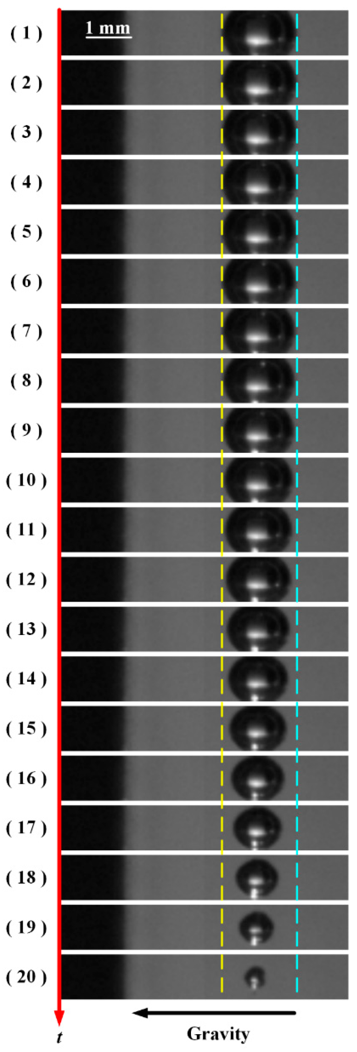
In this section, influences of the bubble–wall distance on the bubble collapse are given in terms of several typical examples in order to describe the main collapsing characteristics of the bubble near the solid wall.

Figure 3, Figure 4 and Figure 5 show the obtained experimental high-speed photos of the dynamic process of the cavitation bubble with short, medium and large distances, respectively. During the bubble collapsing stages with a short distance, one can note that there exist great differences between the movements of the poles A and B of the cavitation bubble interface. Here, in Figure 3, Figure 4 and Figure 5, subplot 1 represents the moment when the cavitation bubble reaches its maximum volume. As for those in Figure 2, the two vertical dashed yellow and blue lines correspond to the bubble positions at maximum volume (R_max), respectively. The time interval between every two adjacent subplots is 4.17 µs. The detailed characteristics among three cases are summarized in

Table 1. Comparisons of the directions and the magnitude of the velocities of the bubble interface poles ($V_A$ and $V_B$) during the bubble collapsing stage in the present experiments.

λ	$\mathbf{Direction}\mathbf{of}{\mathit{V}}_{\mathit{A}}$	$\mathbf{Direction}\mathbf{of}{\mathit{V}}_{\mathit{B}}$	$\Delta \mathit{V}$
Small	No Move	←	Large
Medium	→	←	Medium
Large	→	←	Small

with the following explanations:

Case 1:

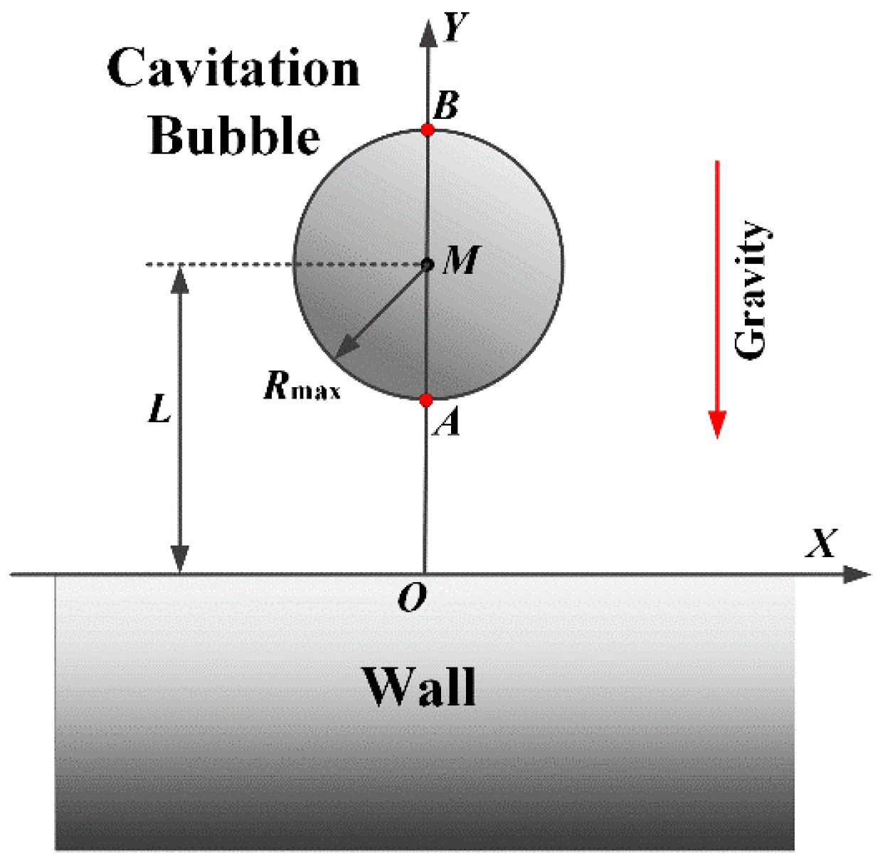
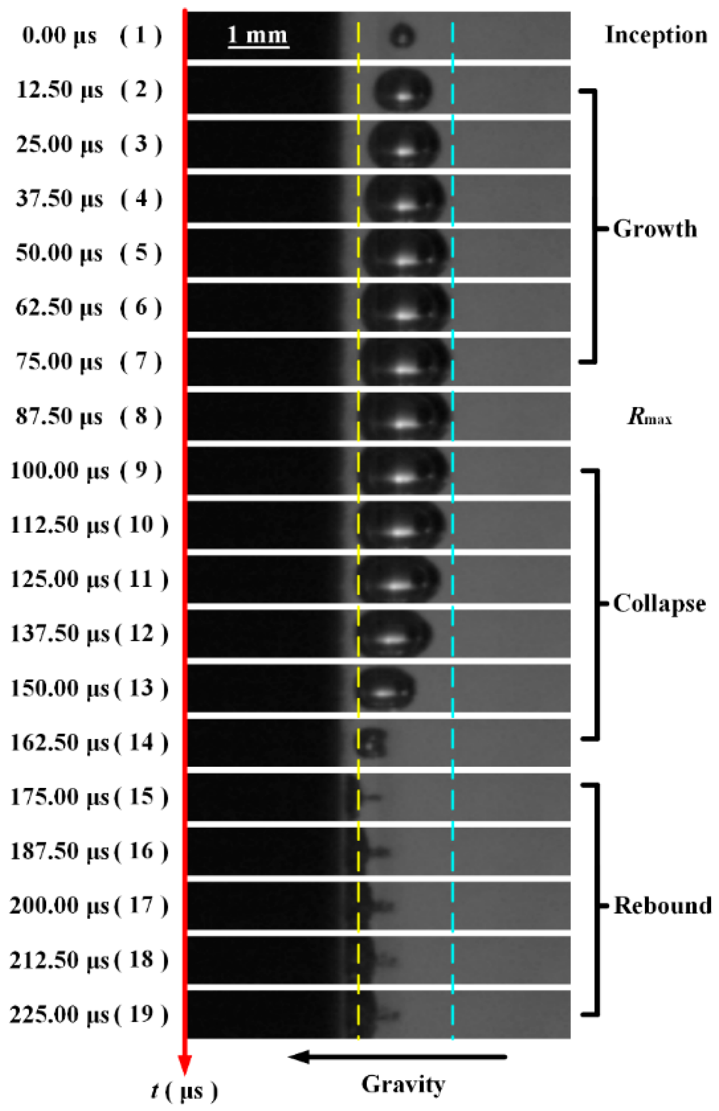
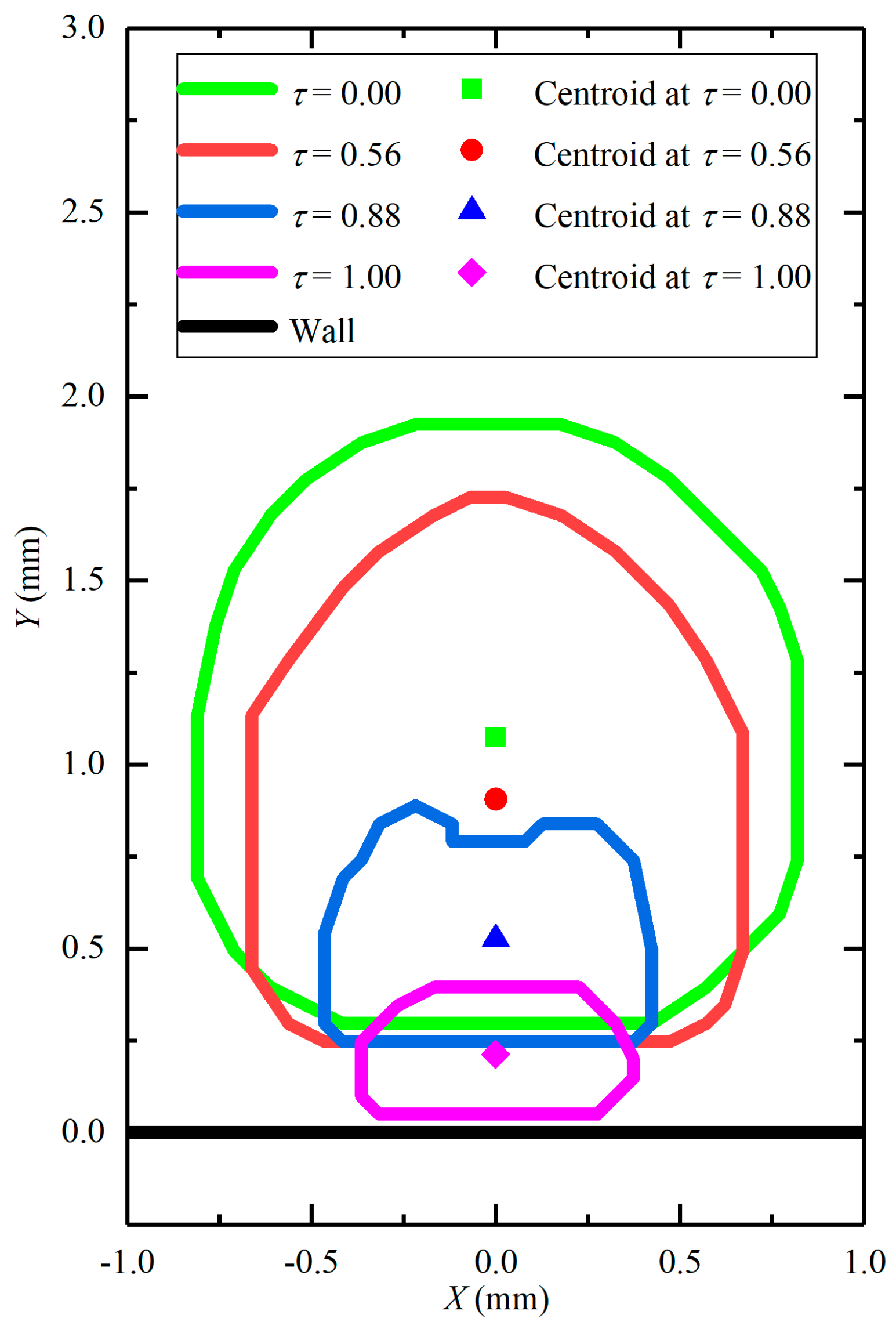
This case corresponds to the condition with a short distance between the cavitation bubble and the wall (e.g., λ = 1.25). It can be observed from the figure that when the cavitation bubble is very close to the wall, pole A is nearly stationary, while pole B moves to the left significantly. In addition, the overall position of the cavitation bubble also moves toward the wall. If the internal density of the cavitation bubbles is assumed to be uniform, the bubble (mass) centroid continuously moves to the left during the collapsing stage. At the end of the collapsing stage (subplot 18–20 in Figure 3), the left side of the bubble approaches the wall surface while the right side of the bubble shows a toroidal shape in the middle, indicating that the jet may be finally generated.

Case 2:

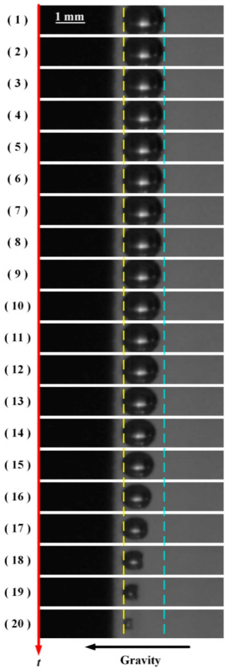
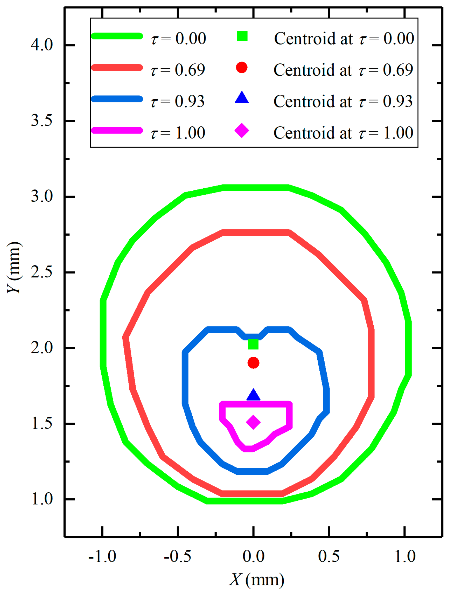
This case corresponds to the condition with a medium distance between the cavitation bubble and the wall (e.g., λ = 2.50). As shown in Figure 4, differently from Figure 3 with a short distance, both poles A and B move towards the inside of the cavitation bubble (Table 1). In addition, the velocity of pole B is much faster than that of pole A, leading to the obvious movement of the bubble towards the wall. Due to the relatively considerable distance, the bubble does not contact the wall during the whole process. At the end of the collapsing stage, similarly to Figure 3, there also exists a toroidal shape on the right side of the cavitation bubble (subplot 20 in Figure 4). However, the display time of the torus is obviously delayed in Figure 4 because of the weak influences of the wall.

Case 3:

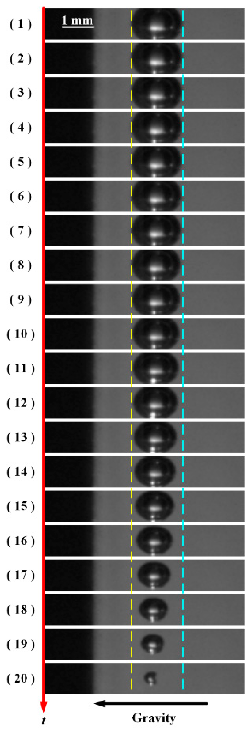
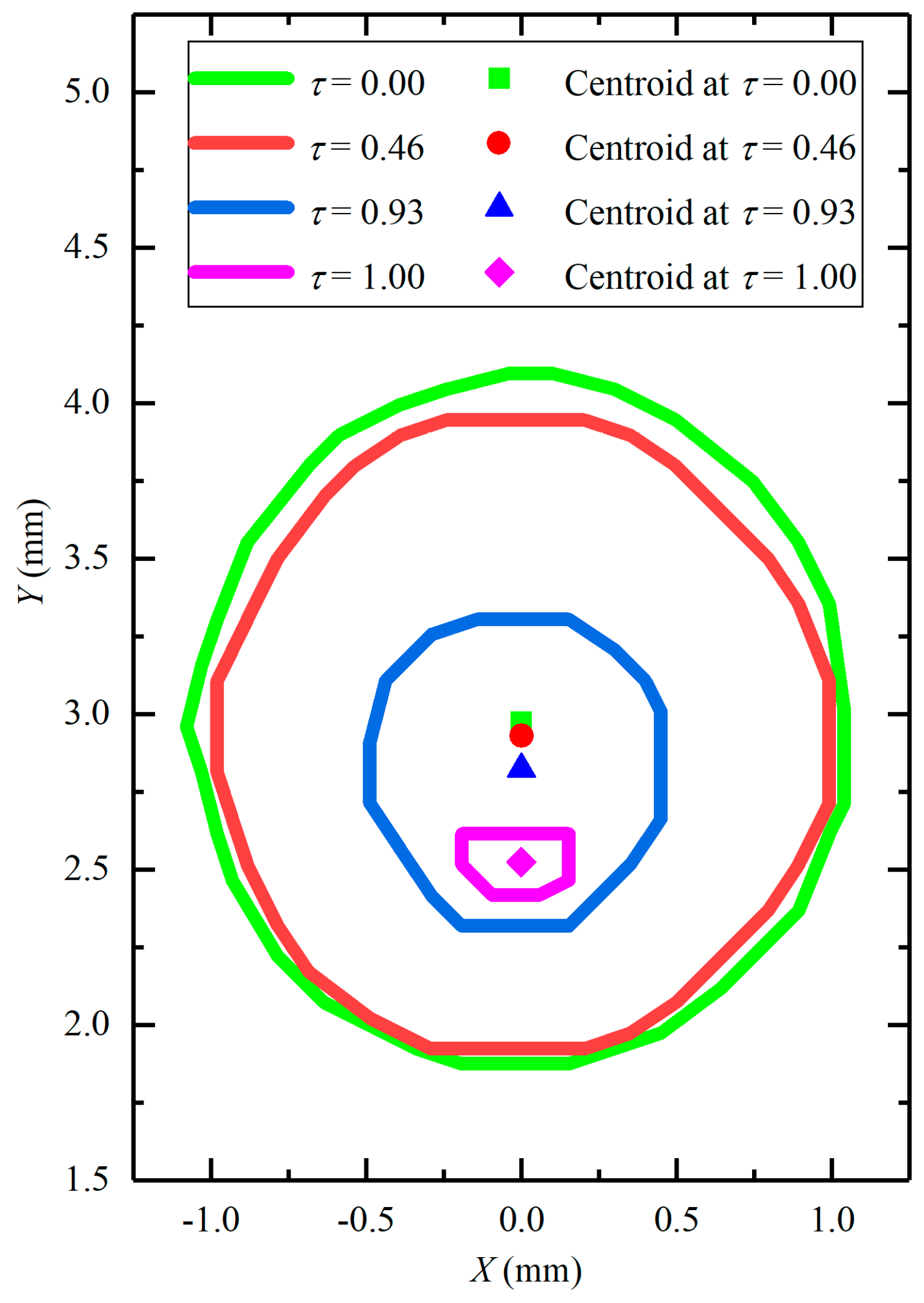
This case corresponds to the condition with a large distance between the cavitation bubble and the wall (e.g., λ = 3.75). It can be observed from the figure that when the bubble–wall distance is large, the bubble nearly retains a spherical shape during the oscillations. In particular, poles A and B both move toward the inside of the bubble with nearly the same speed. Hence, the movement of the bubble centroid is very marginal during the collapsing stage.

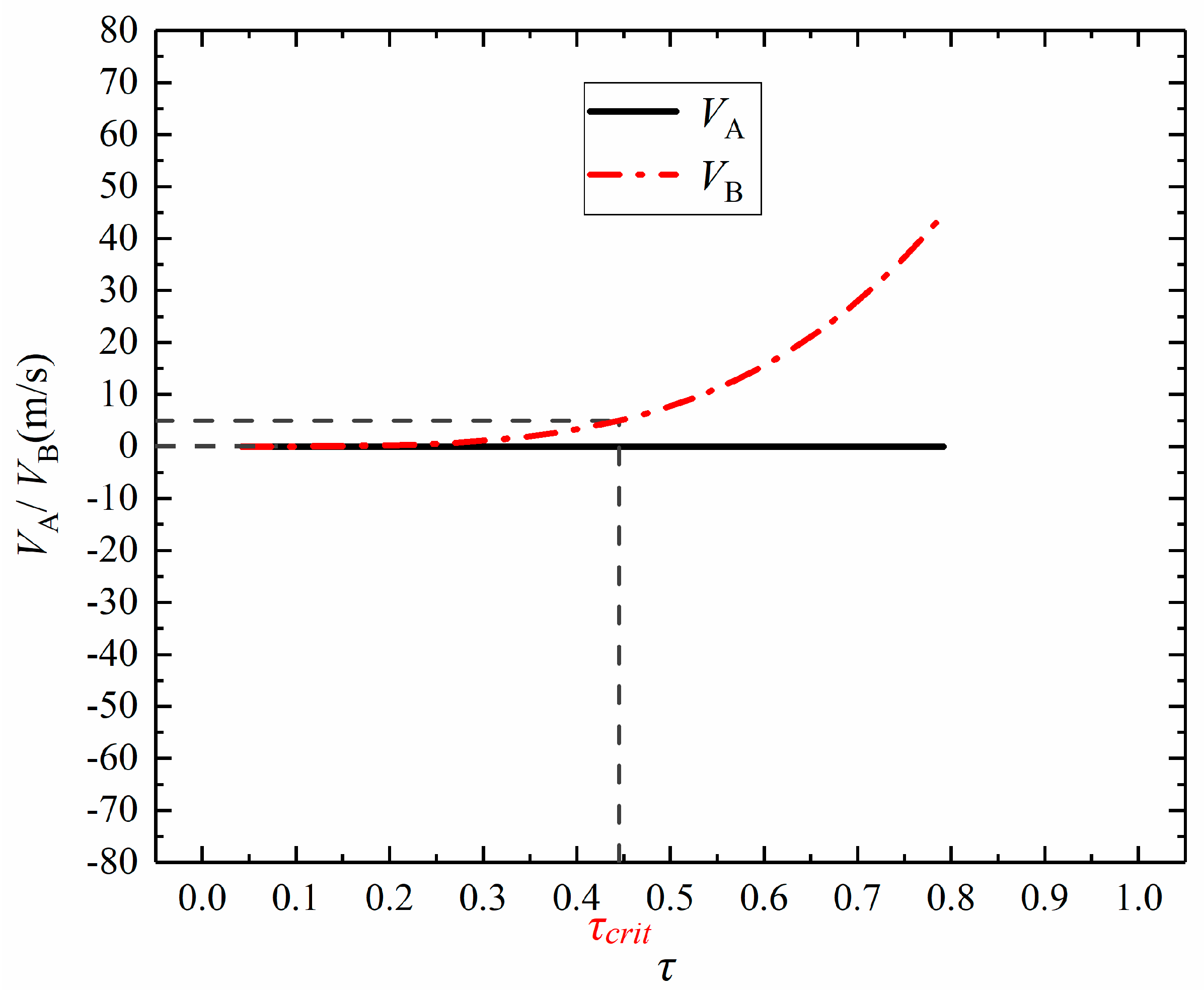
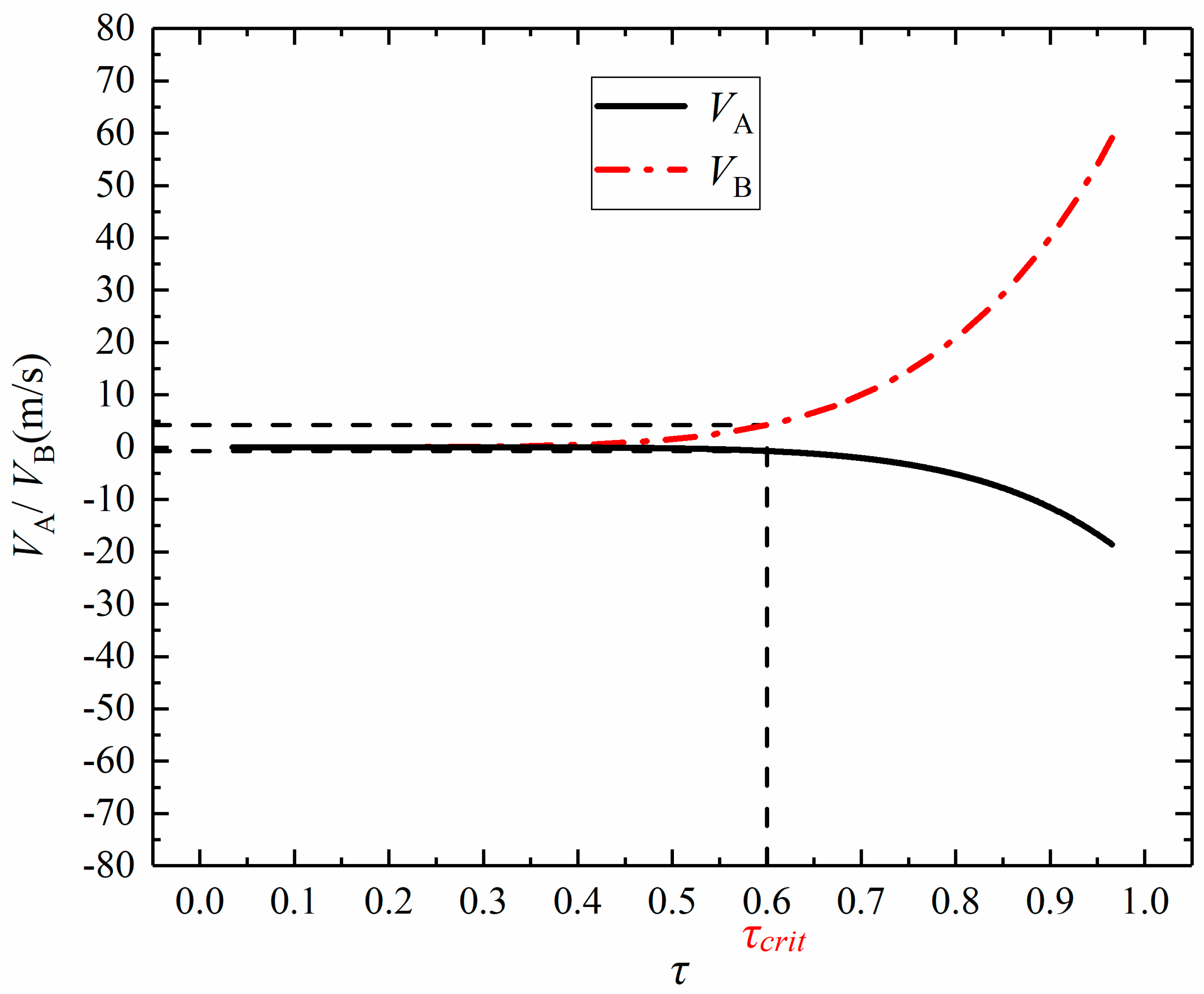
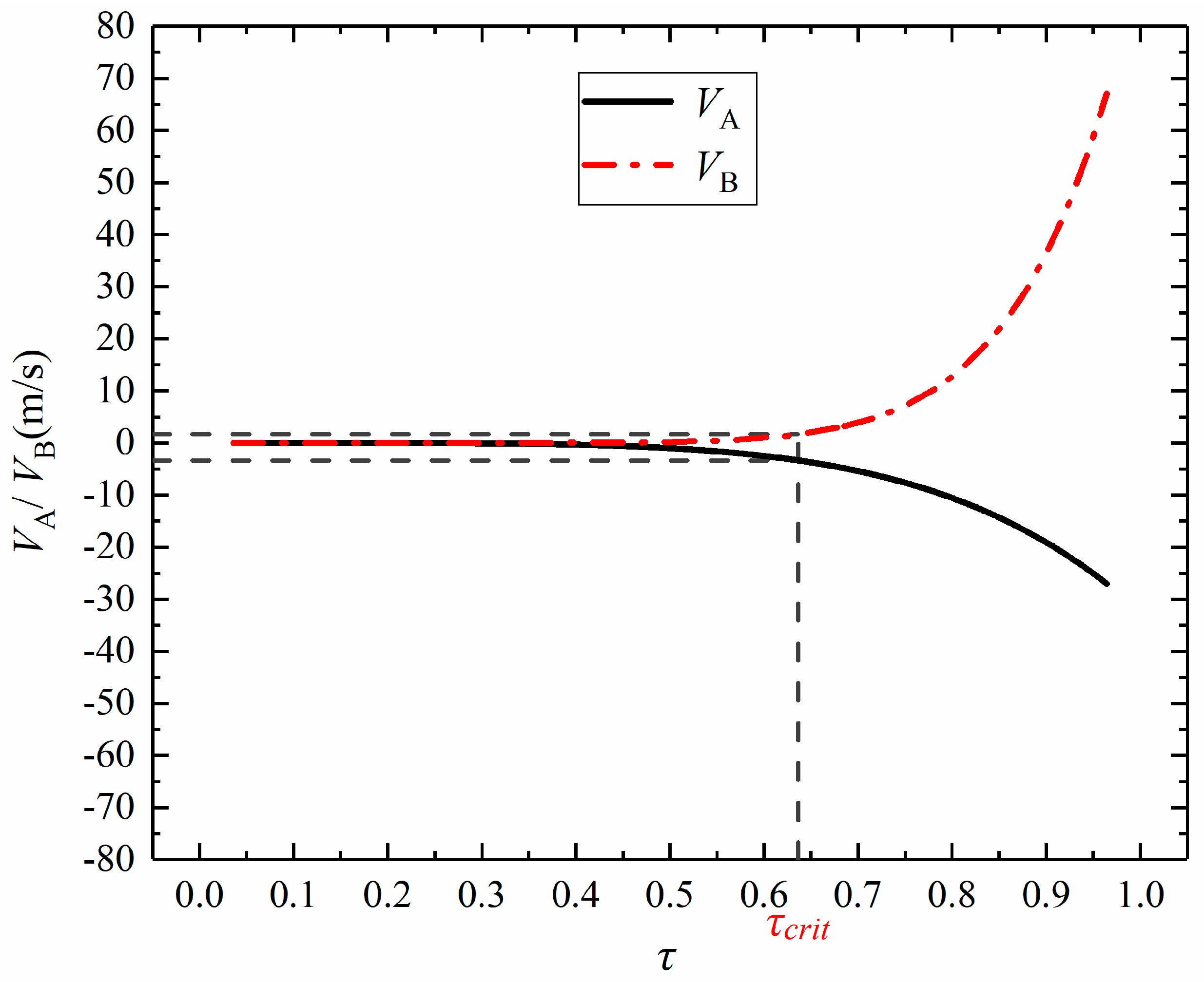
4. The Velocities of Poles A and B of the Cavitation Bubble

In this section, the velocities of poles A and B with different bubble–wall distances will be quantitatively calculated and further discussed in detail. For each subplot, the actual positions of poles A and B during the collapsing stage are accurately evaluated in order to obtain their historical data. Then, based on the obtained data, the velocities of the poles A and B are calculated based on the positions between two frames. Finally, data fitting is employed to show the trends of the curve for the purpose of the comparisons.

Figure 6, Figure 7 and Figure 8 show the variations of the averaged velocities of the poles A and B ($V_A$ and $V_B$) with the non-dimensional collapsing time ($\tau$). The velocities are analyzed based on the experimental data of our previous work [16]. In the figures, the solid black line represents the velocity of pole A ($V_A$), and the dotted-dashed red line represents the velocity of pole B ($V_B$). The positive directions of $V_A$ and $V_B$ are both consistent with the direction of gravity. The τ_crit shown in Figure 6, Figure 7 and Figure 8 is defined as the value of $\tau$ corresponding to a difference in the velocities between poles A and B of 5 m/s.

In order to obtain the trend lines of $V_A$ and $V_B$ accurately, the average velocities of the poles are employed to represent the instantaneous velocities. For the calculations of the velocity curve of the pole, the detailed procedure could be expressed as follows.

Firstly, the present pole positions for a series of the given time are obtained based on the accurate measurement of the poles in each high-speed photo with a time interval ($\Delta \tau$) of 4.17 µs.

Secondly, for the calculations of the average velocity of the pole at a time $\tau$, the moving distance of the pole ($\Delta d$) during the time interval ($\tau -\Delta \tau$, $\tau +\Delta \tau$) is obtained, and then the averaged velocity ($V_i$) is evaluated based on the following expression:

$$V_i=\frac{\Delta d}{2\Delta \tau }$$

(5)

Finally, assuming the velocities are power functions (as shown in Equation (6)), the function fitting method is employed to calculate the coefficients a and b, together with the adjusted $R^2$, during the bubble collapsing stage:

$$V_i=a{\tau }^b$$

(6)

where the subscript i could be A or B.

Table 2. A list of the parameters (including a, b and the adjusted $R^2$) of the fitted lines for the curves of $V_A$ and $V_B$ as shown in Figure 6, Figure 7 and Figure 8.

Parameters	Case 1		Case 2		Case 3
	Point A	Point B	Point A	Point B	Point A	Point B
a	0.00	108.98 ± 18.63	−23.63 ± 3.36	71.81 ± 5.14	−32.40 ± 2.96	92.72 ± 7.60
b	0.00	3.81 ± 0.50	6.82 ± 1.29	5.53 ± 0.54	5.03 ± 0.65	8.88 ± 0.91
Adjusted $R^2$	---	0.90	0.76	0.92	0.88	0.92

shows the coefficients a and b, together with the adjusted $R^2$, for the curves shown in Figure 6, Figure 7 and Figure 8. One can observe that good fits could be obtained in most examples.

Figure 6 shows the velocities of poles A and B for case 1 (with λ = 0.80). When $\tau$ = 0, the velocities of the two poles are almost 0 m/s, corresponding to the condition with the maximum bubble radius. At the early collapsing stage ($\tau$ < 0.30), $V_A$ and $V_B$ are of limited values (nearly zero). For $\tau$ > τ_crit = 0.45, $V_B$ increases dramatically, indicating a large amount of shrinkage. However, $V_A$ is nearly zero throughout and hence it is not necessary to perform curve fitting for $V_A$. Here, because the presence of the torus at the right part of bubble leads to great difficulties for the calculations of $V_B$, only data with $\tau$ < 0.8 is shown in Figure 6. As shown in Figure 6, $\Delta V$ is quite significant for this case, especially at the late collapsing stage.

Figure 7 shows the velocities of poles A and B with λ = 1.59. Compared with case 1, $\tau$ < τ_crit = 0.60, the values of the $V_A$ and $V_B$ are both nearly zero, indicating that the collapse of the bubble is delayed. Furthermore, for $\tau$ > 0.60, $V_A$ also increases slightly but is still far less than $V_B$. For example, at the final collapsing stage ($\tau$ = 1.00), $V_B$ is about three times the value of $V_A$.

Figure 8 shows the velocities of poles A and B with λ = 2.39. As shown in Figure 8, the collapse of the bubble interface is further postponed to $\tau$ > τ_crit = 0.64. Differently from Figure 6 and Figure 7, for nearly the whole collapsing process (e.g., $\tau$ < 0.80), $V_A$ is almost equal to $V_B$ and the bubble mainly retains a spherical collapsing shape (e.g., $V_A\approx V_B$).

As a summary, the retardant effects of the wall on the bubble collapse could be viewed from the non-spherical bubble collapse process. During the collapsing stage of the cavitation bubble, the velocities of the bubble interface in different directions are remarkably different. Specifically, the moving velocity of the interface away from the wall (e.g., pole B) is faster than that near the wall (e.g., pole A). Moreover, the difference between the two velocities ($\Delta V$) increases with the decrease of the standing-off distance.

5. The Motions of the Bubble Centroid

In this section, the contours of the bubble interface and the motions of the centroid of the cavitation bubble during its collapsing stage will be qualitatively and quantitatively discussed. Firstly, Figure 9, Figure 10 and Figure 11 are employed to qualitatively show the movement of the bubble interfaces together with the positions of the bubble centroids for typical phenomenon mentioned in Section 4, respectively. Then, the moving velocities of the bubble centroids during the collapsing stage of the cavitation bubble are further quantitatively discussed.

5.1. The Motions of the Bubble Interface and the Position of the Centroid

Figure 9, Figure 10 and Figure 11 show the motions of the contours of the bubble interfaces and the centroids of the cavitation bubble during its collapsing process ($\tau$ = 0.00–1.00). In the figures, the colored dashed lines represent the contours of the cavitation bubble interface at a given time $\tau$ marked in the figure; the colored symbols with different shapes represent the positions of the bubble centroids of the aforementioned contours with the same color; and the solid black line represents the position of the wall upper surface. Figure 9, Figure 10 and Figure 11 are further analyzed based on the experimental data shown in Figure 6, Figure 7 and Figure 8.

For Figure 9, at the initial stage (e.g., $\tau$ = 0.56), the bubble nearly retains a spherical shape and the movement of the bubble centroid is insignificant. However, at the later stage (e.g., $\tau$ = 0.88 and 1.00), the bubble interfaces show remarkable movement with highly non-spherical shapes. Meanwhile, the bubble centroid also shows considerable movement toward the wall surface.

For Figure 10 and Figure 11, the phenomenon at the initial stage is similar to that of Figure 9. In contrast, for the final collapsing stages, the movement of the bubble centroid is still limited. With the increase of λ, as shown in Figure 10 and Figure 11, the bubble contours are closer to the spherical ones with the bubble centroids nearly unchanged.

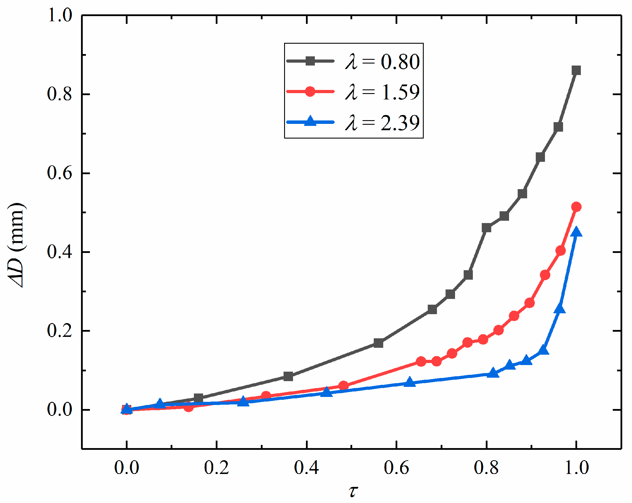
5.2. The Relative Movement of the Bubble Centroid

Figure 12 quantitatively shows the relative movement of the centroid of the cavitation bubble during its whole collapsing stage for Figure 9, Figure 10 and Figure 11. In the figure, the positions of the bubble centroid are calculated based on the high-speed photos obtained during the present experiments. With the decrease of λ, for a given non-dimensional time, the movement of the bubble centroid rapidly increases. The above trends are clearly demonstrated during the whole collapsing process, indicating the strong effects of the wall on the bubble collapsing dynamics.

6. Physical Interpretation of the Phenomenon

In this section, some further discussions of the physical reasons for the observed retardant effects are given. For the large standing-off distance (e.g., case 3), during the bubble growth stage, the bubbles retain a spherical shape, generating a spherically symmetrical fluid flow around the bubble (e.g., the radial flow). In addition, during the bubble interface movement, an outward pressure wave will be also generated and the pressure surrounding the bubble will be increased. Hence, the velocity and the pressure of the fluid around the bubble will be both enhanced prominently. When the bubble reaches its maximum size, the collapse process begins due to the pressure difference across the bubble interface. Because of the spherically symmetrical conditions, the collapse of this case is also spherical.

Now, the case with a short standing-off distance (e.g., case 1) will be analyzed. For the bubble partition away from the wall (denoted “partition 1”), the behavior is similar to that of case 3. However, for the bubble partition near the wall (denoted “partition 2”), the energy of the fluid flow will be greatly dissipated due to the process of the fluid collision with the wall. Hence, both the fluid velocity and the pressure of partition 2 will be lower than those of the other partition (e.g., partition 1). In effect, the pressure inside the bubble could be considered as being uniform. Then, during the collapse, the moving speed of partition 2 will be lower than that of partition 1 due to the different pressure difference across the bubble interface.

The fast-moving velocities of the bubble interface will generate significant shock waves, which could induce a water hammer. Here, the pressure amplitude of the water hammer near the wall can be estimated by employing the following expression adapted from Equation (4) of Ref. [6]:

$$P_{WH}=\frac{{\rho }_L{c}_L{\rho }_W{c}_W}{{\rho }_L{c}_L+{\rho }_W{c}_W}{V}_C.$$

(7)

where $P_{WH}$ is the water hammer (WH) pressure amplitude; ${\rho }_L$ is the density of the surrounding liquid; ${\rho }_W$ is the density of the wall material; $c_L$ is the speed of sound in the surrounding liquid; $c_W$ is the speed of sound in the wall material; and, $V_C$ is the typical bubble collapsing speed. Here, the liquid is water with ${\rho }_L$ of 1000 kg/m³ and $c_L$ of 1500 m/s, and the wall material is steel with ${\rho }_L$ of 8050 kg/m³ and $c_L$ of 5790 m/s. The assumptions employed for Equation (7) include the adiabatic status. In the present paper, the cavitation bubbles show fast movement during the collapse and this assumption could be safely satisfied. As shown in Section 4, a typical collapse velocity ($V_C$) measured in our experiment is of the order of 60 m/s, yielding a rough estimation of $P_{WH}$ of approximately 87.19 MPa. Hence, one can find a vivid example of the tremendous damage potential of the cavitation bubble collapse.

In the above model, the transmission time required for wave propagation is not considered, which is important for a compressible fluid [40]. Here, a rough calculation will be given based on the data of the present setup. The collapse time for the current bubble size is of the order of 100 µs (e.g., 75 µs shown in Figure 2 from inception to R_max). The speed of the wave could be considered to be 1500 m/s, which is the speed of sound in the water. Then, during the bubble collapse, the traveling distance of the wave can be estimated as 0.15 m, which is far beyond the typical size of the generated bubbles (with the maximum bubble radius being about 1 mm). Hence, the pressure wave could easily reach the surrounding fluids near the bubble during its dynamic oscillations. Clearly there are still some limitations of the aforementioned mechanisms (e.g., wave reflections by the wall and the bubble). These complex scenarios will be further considered in future work, together with non-spherical bubble oscillations [41]. Furthermore, the cavitation-induced vortex generations are of great interest for many industrial flows, which could also be revealed with the aid of the newly developed vortex identification method [42,43].

In the future, the discussed theory will be further improved through direct comparisons with other published papers (e.g., those based on the boundary integral method). It should be also noted that there are also some difficulties to be overcome. For example, for the numerical simulations, the choice of the time frame is rather arbitrary (e.g., 0.01 µs shown in Figure 4 in Ref. [38]). During the experiments, for capturing such fine-scale bubble dynamics, a very fast camera is required (e.g., over 100 million fps). Another difficulty for the experiment is the observation of the jet phenomenon. A good flash system with sufficient intensity is necessary, and the synchronization between different systems is also important. These techniques will be attempted in our future work to provide a series of high-quality data.

7. Conclusions

In the present paper, the retardant effects of a wall on bubble interface movement are experimentally investigated with the aid of high-speed photography. Specifically, the influences of the standing-off distance (λ) on the bubble interface contours and the movement of different partitions (represented by poles A and B) are qualitatively and quantitatively revealed, together with the movement of the bubble centroid. The conclusions of the present paper can be summarized as follows:

(1)

The presence of the wall could significantly alter the collapse contour, leading to a great difference between the movements of poles A and B.

(2)

The retardant effect can be observed due to the presence of the wall. With the increase of λ, the retardant effects of the wall will be dismissed and the bubble finally recovers the spherical oscillations.

(3)

The cavitation bubble could induce a significant water hammer pressure (up to 87 MPa in our experiment) during the bubble collapse.

In future work, the retardant effect caused by the wall will be further investigated with the aid of a higher speed camera and a more complex model.

References

1. Zhang, Y.; Liu, K.; Xian, H.; Du, X. A review of methods for vortex identification in hydroturbines. Renew. Sustain. Energy Rev. 2018, 81, 1269–1285. [Google Scholar] [CrossRef]
2. Arndt, R.E.; Voigt, R.L., Jr.; Sinclair, J.P.; Rodrique, P.; Ferreira, A. Cavitation erosion in hydroturbines. J. Hydraul. Eng. 1989, 115, 1297–1315. [Google Scholar] [CrossRef]
3. Brennen, C.E. Hydrodynamics of Pumps; Cambridge University Press: Cambridge, UK, 2011. [Google Scholar]
4. Reuter, F.; Mettin, R. Mechanisms of single bubble cleaning. Ultrason. Sonochem. 2016, 29, 550–562. [Google Scholar] [CrossRef] [PubMed]
5. Zeng, Q.; Gonzalez-Avila, S.R.; Dijkink, R.; Koukouvinis, P.; Gavaises, M.; Ohl, C.D. Wall shear stress from jetting cavitation bubbles. J. Fluid Mech. 2018, 846, 341–355. [Google Scholar] [CrossRef] [Green Version]
6. Philipp, A.; Lauterborn, W. Cavitation erosion by single laser-produced bubbles. J. Fluid Mech. 1998, 361, 75–116. [Google Scholar] [CrossRef]
7. Benjamin, T.B.; Ellis, A.T. The collapse of cavitation bubbles and the pressures thereby produced against solid boundaries. Philos. Trans. R. Soc. Lond. Ser. A 1966, 260, 221–240. [Google Scholar] [CrossRef]
8. Zhang, S.; Duncan, J.H.; Chahine, G.L. The final stage of the collapse of a cavitation bubble near a rigid wall. J. Fluid Mech. 1993, 257, 147–181. [Google Scholar] [CrossRef]
9. Brujan, E.A.; Keen, G.S.; Vogel, A.; Blake, J.R. The final stage of the collapse of a cavitation bubble close to a rigid boundary. Phys. Fluids 2002, 14, 85–92. [Google Scholar] [CrossRef] [Green Version]
10. Popinet, S.; Zaleski, S. Bubble collapse near a solid boundary: A numerical study of the influence of viscosity. J. Fluid Mech. 2002, 464, 137–163. [Google Scholar] [CrossRef]
11. Zhang, Y.L.; Yeo, K.S.; Khoo, B.C.; Wang, C. 3D jet impact and toroidal bubbles. J. Comput. Chem. Phys. 2001, 166, 336–360. [Google Scholar] [CrossRef]
12. Tomita, Y.; Robinson, P.B.; Tong, S.P.; Blake, J.R. Growth and collapse of cavitation bubbles near a curved rigid boundary. J. Fluid Mech. 2002, 466, 259–283. [Google Scholar] [CrossRef]
13. Klaseboer, E.; Hung, K.C.; Wang, C.; Wang, C.W.; Khoo, B.C.; Boyce, P.; Debono, S.; Charlier, H. Experimental and numerical investigation of the dynamics of an underwater explosion bubble near a resilient/rigid structure. J. Fluid Mech. 2005, 537, 387–413. [Google Scholar] [CrossRef]
14. Yusof, N.S.M.; Babgi, B.; Alghamdi, Y.; Aksu, M.; Madhavan, J.; Ashokkumar, M. Physical and chemical effects of acoustic cavitation in selected ultrasonic cleaning applications. Ultrason. Sonochem. 2016, 29, 568–576. [Google Scholar] [CrossRef] [PubMed]
15. Prentice, P.; Cuschieri, A.; Dholakia, K.; Prausnitz, M.; Campbell, P. Membrane disruption by optically controlled microbubble cavitation. Nat. Phys. 2005, 1, 107–110. [Google Scholar] [CrossRef] [Green Version]
16. Zhang, Y.; Xie, X.; Zhang, Y.; Du, X. Experimental study of influences of a particle on the collapsing dynamics of a laser-induced cavitation bubble near a solid wall. Exp. Fluid Sci. 2019, 105, 289–306. [Google Scholar] [CrossRef]
17. Zhang, Y.; Chen, F.; Zhang, Y.; Zhang, Y.; Du, X. Experimental investigations of interactions between a laser-induced cavitation bubble and a spherical particle. Exp. Fluid Sci. 2018, 98, 645–661. [Google Scholar] [CrossRef]
18. Zhang, Y.; Xie, X.; Zhang, Y.; Zhang, Y.X. High-speed experimental photography of collapsing cavitation bubble between a spherical particle and a rigid wall. J. Hydrodyn. 2018, 30, 1012–1021. [Google Scholar] [CrossRef]
19. Gonzalez-Avila, S.R.; Klaseboer, E.; Khoo, B.C.; Ohl, C.D. Cavitation bubble dynamics in a liquid gap of variable height. J. Fluid Mech. 2011, 682, 241–260. [Google Scholar] [CrossRef]
20. Brujan, E.A.; Takahira, H.; Ogasawara, T. Planar jets in collapsing cavitation bubbles. Exp. Fluid Sci. 2019, 101, 48–61. [Google Scholar] [CrossRef]
21. Li, T.; Zhang, A.M.; Wang, S.P.; Li, S.; Liu, W.T. Bubble interactions and bursting behaviors near a free surface. Phys. Fluids 2019, 31, 042104. [Google Scholar] [CrossRef]
22. Pearson, A.; Cox, E.; Blake, J.R.; Otto, S.R. Bubble interactions near a free surface. Eng. Anal. Bound. Elem. 2004, 28, 295–313. [Google Scholar] [CrossRef]
23. Brujan, E. Cavitation in Non-Newtonian Fluids: With Biomedical and Bioengineering Applications; Springer: Berlin/Heidelberg, Germany, 2010. [Google Scholar]
24. Brujan, E.A.; Nahen, K.; Schmidt, P.; Vogel, A. Dynamics of laser-induced cavitation bubbles near an elastic boundary. J. Fluid Mech. 2001, 433, 251–281. [Google Scholar] [CrossRef]
25. Hopfes, T.; Wang, Z.; Giglmaier, M.; Adams, N.A. Collapse dynamics of bubble pairs in gelatinous fluids. Exp. Fluid Sci. 2019, 108, 104–114. [Google Scholar] [CrossRef]
26. Wu, J.H.; Wang, Y.; Ma, F.; Gou, W.J. Cavitation erosion in bloods. J. Hydrodyn. 2017, 29, 724–727. [Google Scholar] [CrossRef]
27. Wan, C.R.; Liu, H. Shedding frequency of sheet cavitation around axisymmetric body at small angles of attack. J. Hydrodyn. 2017, 29, 520–523. [Google Scholar] [CrossRef]
28. Blake, J.R.; Gibson, D.C. Cavitation bubbles near boundaries. Annu. Rev. Fluid Mech. 1987, 19, 99–123. [Google Scholar] [CrossRef]
29. Lauterborn, W.; Kurz, T. Physics of bubble oscillations. Rep. Prog. Phys. 2010, 73, 106501. [Google Scholar] [CrossRef]
30. Brennen, C.E. Cavitation and Bubble Dynamics; Cambridge University Press: Cambridge, UK, 1995. [Google Scholar]
31. Wang, S.P.; Zhang, A.M.; Liu, Y.L.; Zhang, S.; Cui, P. Bubble dynamics and its applications. J. Hydrodyn. 2018, 30, 975–991. [Google Scholar] [CrossRef]
32. Best, J.P. The formation of toroidal bubbles upon the collapse of transient cavities. J. Fluid Mech. 1993, 251, 79–107. [Google Scholar] [CrossRef]
33. Lee, M.; Klaseboer, E.; Khoo, B.C. On the boundary integral method for the rebounding bubble. J. Fluid Mech. 2007, 570, 407–429. [Google Scholar] [CrossRef]
34. Wang, Q. Multi-oscillations of a bubble in a compressible liquid near a rigid boundary. J. Fluid Mech. 2014, 745, 509–536. [Google Scholar] [CrossRef]
35. Wang, Q.; Liu, W.; Zhang, A.M.; Sui, Y. Bubble dynamics in a compressible liquid in contact with a rigid boundary. Interface Focus 2015, 5, 20150048. [Google Scholar] [CrossRef] [PubMed]
36. Han, R.; Zhang, A.M.; Li, S.; Zong, Z. Experimental and numerical study of the effects of a wall on the coalescence and collapse of bubble pairs. Phys. Fluids 2018, 30, 042107. [Google Scholar] [CrossRef]
37. Koch, M.; Lechner, C.; Reuter, F.; Köhler, K.; Mettin, R.; Lauterborn, W. Numerical modeling of laser generated cavitation bubbles with the finite volume and volume of fluid method, using OpenFOAM. Comput. Fluids 2016, 126, 71–90. [Google Scholar] [CrossRef]
38. Lechner, C.; Lauterborn, W.; Koch, M.; Mettin, R. Fast, thin jets from bubbles expanding and collapsing in extreme vicinity to a solid boundary: A numerical study. Phys. Rev. Fluids 2019, 4, 021601. [Google Scholar] [CrossRef]
39. Thoroddsen, S.T.; Etoh, T.G.; Takehara, K. High-speed imaging of drops and bubbles. Annu. Rev. Fluid Mech. 2008, 40, 257–285. [Google Scholar] [CrossRef]
40. Wang, Q.; Liu, W.; Leppinen, D.M.; Walmsley, A.D. Microbubble dynamics in a viscous compressible liquid near a rigid boundary. IMA J. Appl. Math. 2019, 84, 696–711. [Google Scholar] [CrossRef]
41. Klapcsik, K.; Hegedűs, F. Study of non-spherical bubble oscillations under acoustic irradiation in viscous liquid. Ultrason. Sonochem. 2019, 54, 256–273. [Google Scholar] [CrossRef] [PubMed]
42. Zhang, Y.; Qiu, X.; Chen, F.; Liu, K.; Zhang, Y.; Liu, C. A selected review of vortex identification methods with applications. J. Hydrodyn. 2018, 30, 767–779. [Google Scholar] [CrossRef]
43. Dong, X.; Wang, Y.; Chen, X.; Dong, Y.; Zhang, Y.; Liu, C. Determination of epsilon for Omega vortex identification method. J. Hydrodyn. 2018, 30, 541–548. [Google Scholar] [CrossRef]
Figure 1. The definitions of the paramount control parameters of the bubble–wall interaction system. In the figure, L is the distance between the inception point of the cavitation bubble and the upper surface of the wall; Rmax is the equivalent maximum radius of the bubble during its whole oscillations. The red arrow represents the direction of gravity.
Symmetry 11 01051 g001
Figure 2. Representative high-speed photos of the dynamic process of the cavitation bubble near the wall from the bubble inception to the rebound. fps = 240,000, λ = 1.00.
Symmetry 11 01051 g002
Figure 3. The obtained experimental high-speed photos of the dynamic process of the cavitation bubble with a short distance to the wall. The time interval between two adjacent subplots is 4.17 µs. The two vertical dashed yellow and blue lines correspond to the bubble positions during the maximum volume, respectively. fps = 240,000, λ = 1.25.
Symmetry 11 01051 g003
Figure 4. The obtained experimental high-speed photos of the dynamic process of the cavitation bubble with a medium distance to the wall. The time interval between two adjacent subplots is 4.17 µs. The two vertical dashed yellow and blue lines correspond to the bubble positions during the maximum volume, respectively. fps = 240,000, λ = 2.50.
Symmetry 11 01051 g004
Figure 5. The obtained experimental high-speed photos of the dynamic process of the cavitation bubble with a large distance to the wall. The time interval between two adjacent subplots is 4.17 µs. The two vertical dashed yellow and blue lines correspond to the bubble positions during the maximum volume respectively. fps = 240,000, λ = 3.75.
Symmetry 11 01051 g005
Figure 6. The velocities of the poles A and B of the cavitation bubble interface during the collapsing stage with a short bubble–wall distance (λ = 0.80). The solid black line represents the velocity of pole A ( V A ) and the dotted-dashed red line represents the velocity of pole B ( V B ).
Symmetry 11 01051 g006
Figure 7. The velocities of the poles A and B of the cavitation bubble interface during the collapsing stage with a medium bubble–wall distance (λ = 1.59). The solid black line represents the velocity of pole A ( V A ) and the dotted-dashed red line represents the velocity of pole B ( V B ).
Symmetry 11 01051 g007
Figure 8. The velocities of the poles A and B of the cavitation bubble interface during the collapsing stage with a large bubble–wall distance (λ = 2.39). The solid black line represents the velocity of pole A ( V A ) and the dotted-dashed red line represents the velocity of pole B ( V B ).
Symmetry 11 01051 g008
Figure 9. The motions of the bubble interface and the movement of the bubble centroid during the collapsing stage with λ = 0.80. The four dashed lines with different colors represent the four representative interfaces of the cavitation bubble during its collapsing stage (τ = 0.00–1.00). The four symbols with different colors and shapes represent the calculated centroids of the cavitation bubbles for the given non-dimensional time. The black line represents the position of the wall.
Symmetry 11 01051 g009
Figure 10. The motions of the bubble interface and the movement of the bubble centroid during the collapsing stage with λ = 1.59. The four dashed lines with different colors represent the four representative interfaces of the cavitation bubble during its collapsing stage (τ = 0.00–1.00). The four symbols with different colors and shapes represent the calculated centroids of the cavitation bubbles for the given non-dimensional time. The black line represents the position of the wall.
Symmetry 11 01051 g010
Figure 11. The motions of the bubble interface and the movement of the bubble centroid during the collapsing stage with λ = 2.39. The four dashed lines with different colors represent the four representative interfaces of the cavitation bubble during its collapsing stage (τ = 0.00–1.00). The four symbols with different colors and shapes represent the calculated centroids of the cavitation bubbles for the given non-dimensional time. The black line represents the position of the wall.
Symmetry 11 01051 g011
Figure 12. The variations of the moving distance ( Δ D ) of the bubble centroids with non-dimensional time (τ) during the collapsing stage.
Symmetry 11 01051 g012