Article

An Improved Butterfly Optimization Algorithm for Engineering Design Problems Using the Cross-Entropy Method

1
School of Finance and Mathematics, West Anhui University, Lu’an 237012, China
2
Department of Mechanical and Aerospace Engineering, University of Florida, Gainesville, FL 32611, USA
3
School of Economics and Management, East China Jiaotong University, Nanchang 330013, China
*
Authors to whom correspondence should be addressed.
Symmetry 2019, 11(8), 1049; https://doi.org/10.3390/sym11081049
Submission received: 4 July 2019 / Revised: 9 August 2019 / Accepted: 9 August 2019 / Published: 14 August 2019
(This article belongs to the Special Issue Symmetry in Mechanical Engineering)

Abstract

:
Engineering design optimization in real life is a challenging global optimization problem, and many meta-heuristic algorithms have been proposed to obtain the global best solutions. An excellent meta-heuristic algorithm has two symmetric search capabilities: local search and global search. In this paper, an improved Butterfly Optimization Algorithm (BOA) is developed by embedding the cross-entropy (CE) method into the original BOA. Based on a co-evolution technique, this new method achieves a proper balance between exploration and exploitation to enhance its global search capability, and effectively avoid it falling into a local optimum. The performance of the proposed approach was evaluated on 19 well-known benchmark test functions and three classical engineering design problems. The results of the test functions show that the proposed algorithm can provide very competitive results in terms of improved exploration, local optima avoidance, exploitation, and convergence rate. The results of the engineering problems prove that the new approach is applicable to challenging problems with constrained and unknown search spaces.

1. Introduction

Real-world engineering design optimization problems are very challenging to find the global optimum of a highly complex and multiextremal objective function, involving many different decision variables under complex constraints [1,2]. A general engineering design optimization problem can be stated as follows:
min f ( x ) , x = ( x 1 , x 2 , , x n ) T R n ,
subject to
g j ( x ) 0 , j = 1 , 2 , , p ,
h k ( x ) = 0 , k = 1 , 2 , , q ,
l b i x i u b i , i = 1 , 2 , , n ,
where n is the number of search space dimensions, g j ( x ) and h k ( x ) are the jth inequality constraint and kth equality constraint, respectively. l b i and u b i represent the lower and upper bound of the value of x i .
Most of the constraints of the global optimization problem are nonlinear. Such nonlinearity often results in a multimodal response landscape [3]. Due to their high complexity, nonlinearity, and multimodality, traditional optimization methods, such as gradient-based optimization algorithms, are no longer suitable for this problem [4]. Many researchers have developed various derivative-free global optimization methods for it. In general, these methods can be divided into two classes: deterministic methods and stochastic meta-heuristic algorithms [4,5]. The former, such as the Hill-Climbing [6], Newton–Raphson [7], and DIRECT algorithm [8], can obtain the same optimal results based on the same set of initial values. However, this behavior results in local optima entrapment and a loss of reliability in finding the global optimum, since most real engineering design problems have extremely high numbers of local solutions [9]. The latter, such as the Genetic Algorithm (GA) [10,11], Particle Swarm Optimization (PSO) [12], Cuckoo Search (CS) [13], Bat Algorithm (BA) [14], Grey Wolf Optimizer (GWO) [15], Forest Optimization Algorithm (FOA) [16,17], Ant Lion Optimizer (ALO) [9], Whale Optimization Algorithm (WOA) [18], Crow Search Algorithm (CSA) [19], Salp Swarm Algorithm (SSA) [20], and Butterfly Optimization Algorithm (BOA) [21,22], mostly benefit from their simplicity, flexibility, and stochastic operators, which makes them different from deterministic methods [4], and they have become very popular optimization techniques for such optimization problems in recent years.
Despite the merits of nature-inspired meta-heuristic algorithms, it has been pointed out that most of them are unable to guarantee global convergence [23]. At the same time, the No Free Lunch (NFL) theorem has proved that none of these methods are able to solve all global optimization problems [24]. They perform very well when dealing with certain optimization problems, but fail in most cases. An excellent meta-heuristic algorithm has two symmetric search capabilities: local search and global search, and achieves a proper balance between exploration and exploitation to effectively avoid it falling into a local, and find the global optimum. In order to enhance global search capabilities, many hybrid meta-heuristic algorithms have been developed by combining meta-heuristics with exact algorithms or other meta-heuristics for solving more complicated optimization problems [25,26,27,28,29].
Inspired by the idea of global random search algorithms [5,30], and based on co-evolution, this paper explores an improved butterfly optimization algorithm (BOA) using the cross-entropy method, which is a global stochastic optimization method based on a statistical model. The original BOA was proposed by Arora and Singh [21] in 2015, and was inspired by the food foraging behavior of butterflies, while the cross-entropy (CE) method was developed by Rubinstein [31] in 1997 to estimate the probability of rare events in complex random networks. Since the BOA has a tendency to prematurely converge to local optima [32], this paper embeds the CE method into the BOA to obtain a good balance between exploration and exploitation and improve the BOA’s global search capability.
The rest of this paper is structured as follows. In Section 2, the BOA and CE method are briefly introduced, and a study of the improved BOA is presented in Section 3. The results and a discussion of benchmark functions are provided in Section 4. Section 5 solves three classical engineering design problems. In Section 6, conclusions and future research directions are presented.

2. Methods

2.1. Butterfly Optimization Algorithm

The BOA is a new nature-inspired meta-heuristic algorithm which was inspired by the food foraging behavior of butterflies [21,22]. In this method, the characteristics of butterflies are ideally summarized as follows:
1. All butterflies are assumed to emit some fragrance that makes the butterflies attractive to each other;
2. Each butterfly moves randomly or toward the best butterfly—i.e., the one which emits the most fragrance;
3. The stimulus intensity of a butterfly is determined by the landscape of the objective function.
In the BOA, the perceived magnitude of the fragrance (f) is defined as a function of the stimulus physical intensity as follows:
f = c I a ,
where c [ 0 , ] is the sensory modality; I is the stimulus intensity, which is associated with the encoded objective function; and a [ 0 , 1 ] is the power exponent dependent on modality, which represents the varying degree of fragrance absorption.
There are two key steps in the BOA: global search and local search. The former can make the butterflies move toward the best butterfly, which can be represented as
x i t + 1 = x i t + ( r 2 × g x i t ) × f i ,
where x i t is the position of the ith butterfly at time t. Here, g represents the current best position. f i represents the fragrance of the ith butterfly, and r is a random number in [ 0 , 1 ] .
The latter is implemented through a local random walk, which can be represented as
x i t + 1 = x i t + ( r 2 × x j t x k t ) × f i ,
where x j t and x k t are the positions of the jth and kth butterflies in the solution space, respectively, and r is a random number in [ 0 , 1 ] .
Additionally, a switch probability p is used in the BOA to switch between a common global search and an intensive local search. Based on the above, the original BOA can be implemented with pseudo-code as shown in Algorithm 1:
Algorithm 1: Butterfly Optimization Algorithm
  Begin
   Objective function f ( x ) , x = ( x 1 , x 2 , , x d ) T , here d represents the number of dimensions.
   Generate initial population P containing n butterflies p o p i ( i = 1 , 2 , , n ) .
   Stimulus I i intensity at is p o p i determined by the fitness value f ( p o p i ) .
   Define sensor modality c, power exponent a, and switch probability p.
   while stop criteria not met do
        for each butterfly in the population P do
             Calculate fragrance f using Equation (5).
        end for
        Evaluate and rank the population P, and find the best butterfly.
        for each butterfly in the population P do
             Generate a random number r U [ 0 , 1 ] .
             if ( r < p )
                  Implement global search using Equation (6).
             else
                  Implement local search using Equation (7).
             end if
        end for
        Update the value of the power exponent a.
   end while
   Output the best solution and optimal value.
End
BOA shows better performance compared to some other optimization algorithms [21,22] and has attracted the attention of many researchers due to its simplicity and interesting nature-inspired interpretations as an optimization approach for global optimization problems and for various real-life applications [32,33].

2.2. The Cross-Entropy (CE) Method

Based on Monte Carlo technology, Rubinstein [31] developed the CE method in 1997 and uses the cross-entropy or Kullback–Leibler divergence to measure the distance between two sampling distributions, solve an optimization problem by minimizing this distance, and obtain the optimal parameters of probability distribution. The CE method has good global search capability, excellent adaptability, and strong robustness. It is frequently used for many complex optimization problems such as continuous multi-extremal optimization [34], multi-objective optimization [35], combination optimization [36,37], vehicle routing problems [38], energy-efficient radio resource management [39], and complex optimization problems from other fields [40,41,42,43].
A general optimization problem can be stated as follows:
min x X S ( x ) ,
where X is a finite set of states, and S is a real-valued performance function on X .
Next, we can construct a probability distribution estimation problem associated with the above problem, and the auxiliary problem can be defined as follows:
l ( γ ) = P u ( S ( X ) γ ) = E u [ I { S ( X ) γ } ] ,
where P u is the probability measure under which the random state X has some probability density function f ( x ; u ) on X ; E u is the corresponding expectation operator; γ represents a threshold parameter; and I represents the indicator function, whose value is 1, if S ( X ) γ , and 0, otherwise. The importance sampling approach is used to reduce the sample size in the CE method. Consequently, Equation (9) can be rewritten as follows:
l ( γ ) = 1 N i = 1 N I S ( X ) γ f ( x i ; v ) g ( x i ) ,
where x i represents a random sample from f ( x ; v ) with importance sampling density g ( x ) . the Kullback–Leibler divergence, i.e., the cross-entropy is introduced to measure the distance between two sampling distributions for obtaining the optimal importance sampling density. Thus, the optimal density g ( x ) can be found by minimizing the Kullback–Leibler divergence, which is equivalent to solving the following optimization problem [34]:
min v 1 N i = 1 N I S ( X ) γ ln f ( x i ; v ) .
In order to improve the convergence speed of the CE method, adaptive smoothing v ^ k is demoted by v ˜ , as follows:
v ^ k + 1 = α v ˜ + ( 1 α ) v ^ k ,
where 0 α 1 is a smoothing parameter.
The CE method for optimization problems is described in Algorithm 2.
Algorithm 2: Cross-entropy (CE) for optimization problems
  Begin
   Set t = 0 . Initialize the probability parameter v ^ k .
   while stop criteria for CE not met do
        Generate S 1 , S 2 , , S N i i d f ( x ; v ^ k ) . Evaluate and rank the sample S.
        Solve the problem given in Equation (11) based on the sample S. Denote the solution by  v ˜ .
        Update the parameter v ^ k using v ˜ .
        Set t = t + 1 .
   end while
   Output the best solution and optimal value.
End

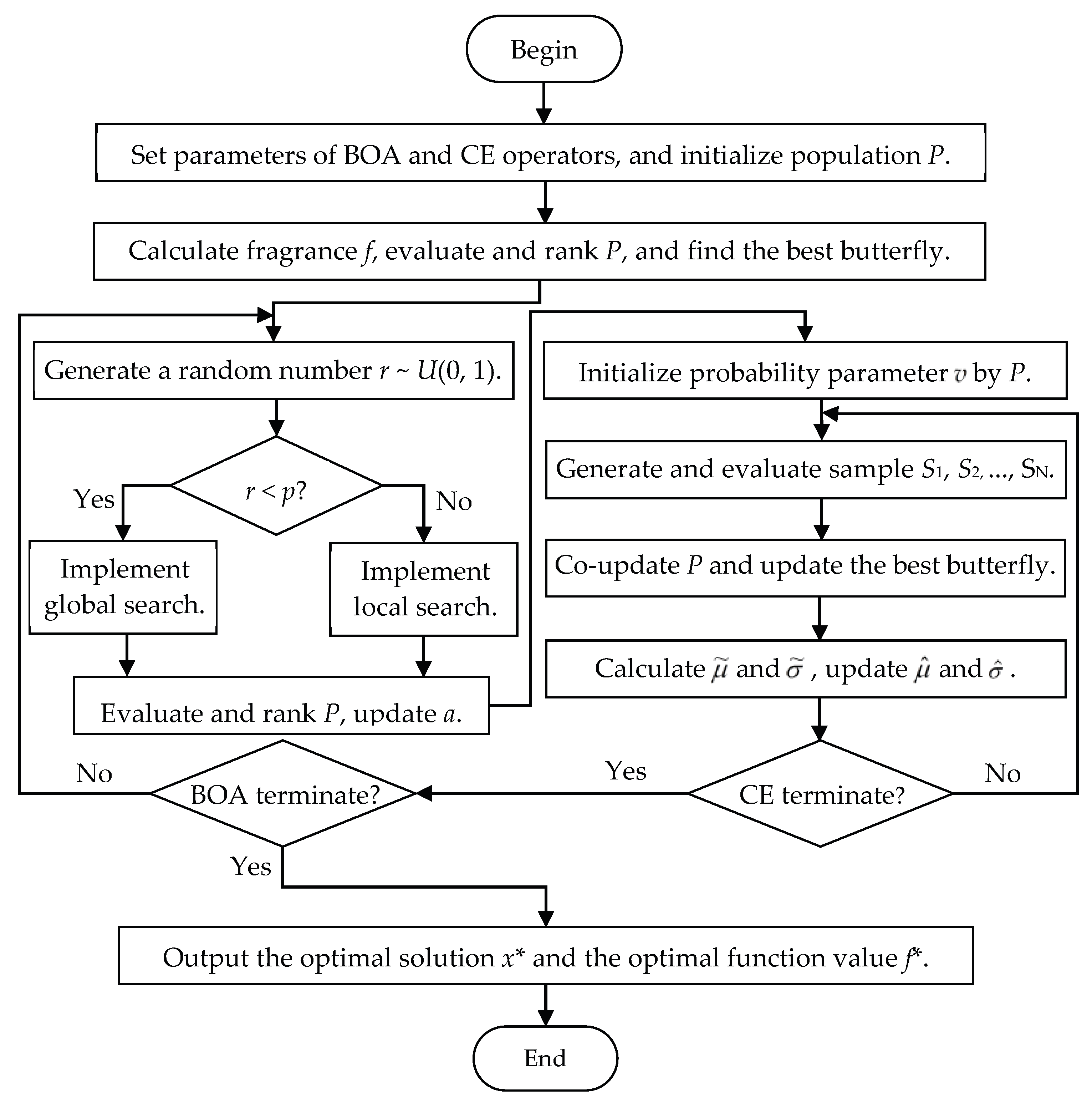
3. Hybrid BOA-CE Method

This section presents the details of the improved algorithm, named BOA-CE. A meta-heuristic method should have two main functions—exploration and exploitation—and should try to find a proper balance between them for better performance [44]. The nature-inspired BOA has shown the advantages of excellent local search capability and fast convergence; however, it tends to fall into a local optimum rather than finding the global optimum [21,22,32,33]. In order to improve the global search capability of the BOA, and, based on a co-evolutionary technique, this paper proposes the BOA-CE algorithm by embedding the CE method into it. The new method contains BOA and CE optimization operators, and co-updates the BOA population P and the CE sample S using co-evolutionary technology in each iteration. The CE operator obtains the initial probability parameters using the BOA population P in order to improve its convergence rate while the BOA operator updates its population P and the best butterfly using the elite sample S e of the CE operator to enhance the population diversity. The pseudo-code of the BOA-CE hybrid algorithm is described in Algorithm 3. Figure 1 presents the flow chart of the BOA-CE algorithm, and the co-evolutionary process between BOA operator and CE operator can be clearly seen from Figure 1.
In addition, as an example, we use the BOA-CE algorithm to find the global optimum of the 2D Sphere function in order to more clearly describe the co-evolutionary process of the BOA operator and the CE operator:
f ( x ) = x 1 2 + x 2 2 , 100 x 1 , x 2 100 ,
which has a global minimum f = 0 at x = ( 0 , 0 ) T . Now, let us use the BOA-CE algorithm to find the optima and this process is summarized as follows: (1) the values of the parameters of the BOA operator are c = 0.01 , a = 0.1 , p = 0.8 , the population size n = 40 , and the maximum number of iteration t 1 = 50 , while the values of the parameters of the CE operator are α = 0.8 , the sample size N = 80 , the elite sample size N e = 30 , and the maximum number of iteration t 2 = 2 ; (2) initializing the population of the BOA operator P, calculating f i ( x ) = x i 1 2 + x i 2 2 , i = 1 , 2 , , 40 , and finding the current best f = 13.5036 and x = ( 3.5586 , 0.9164 ) T ; (3) generating a rand number r, and updating x i with x i n e w = x i o l d + ( r 2 × f x i o l d ) × f i if r p and x i n e w = x i o l d + ( r 2 × x j o l d x k o l d ) × f i otherwise for each butterfly in the P; (4) calculating the mean μ = ( 4.9571 , 11.4528 ) and standard σ = ( 60.2592 , 53.9977 ) deviation of P, and using them to initialize the probability parameter v = ( 4.9571 , 11.4528 , 60.2592 , 53.9977 ) ; (5) generating a sample S by the probability parameter v, and calculating f i ( x ) = x i 1 2 + x i 2 2 , i = 1 , 2 , , 80 , and finding the new current best f = 4.4290 and x = ( 1.8693 , 0.9668 ) T ; (6) updating the probability parameter v using the elite sample, and regenerating a sample S using the new parameter v, and finding the new current best f = 2.4542 and x = ( 0.8951 , 1.2857 ) T ; (7) co-updating the population P using the sample S and the population P; (8) repeating the above operations until the termination condition ( t 1 > 50 ) is met, and outputting the approximate optimal solution x = ( 1.1154 × 10 31 , 2.5727 × 10 32 ) T and function value f = 1.3104 × 10 62 . Figure 2 clearly describes the of co-updating the current best f by the BOA operator and CE operator.
Algorithm 3: BOA-CE algorithm
  Begin
   Objective function f ( x ) , x = ( x 1 , x 2 , , x d ) T ; here, d represents the number of dimensions.
   Generate initial population P containing n butterflies p o p i ( i = 1 , 2 , , n ) .
   Stimulus I i intensity at is p o p i determined by the fitness value f ( p o p i ) .
   Define sensor modality c, power exponent a, and switch probability p.
   while stop criteria not met do
        for each butterfly in the population P do
             Calculate fragrance f using Equation (5).
        end for
        Evaluate, rank P, and find the best butterfly.
        for each butterfly in the population P do
             Generate a random number r U [ 0 , 1 ] .
             if ( r < p )
                  Implement global search using Equation (6).
             else
                  Implement local search using Equation (7).
             end if
        end for
        Update the value of the power exponent a.
        Evaluate and rank the population P.
        Initialize the probability parameter v ^ k using the population P.
        while stop criteria for CE not met do
             Generate S 1 , S 2 , , S N i i d f ( x ; v ^ k ) , evaluate the sample S.
             Rank the population P and the sample S together, co-update P and S, update the best butterfly.
             Calculate the probability parameter v ˜ by the elite sample S e .
             Update the probability parameters v ^ k via Equation (12).
        end while
   end while
   Output the best solution and optimal value.
End
The BOA-CE hybrid algorithm has two main operators: BOA and CE. The BOA operator has two inner loops for the butterflies population size n 1 , and one outer loop for iteration t 1 . While the CE operator has one inner loops for the sample size n 2 , and two outer loops for iterations t 1 and t 2 , respectively. Therefore, for our proposed hybrid algorithm (BOA-CE), the time complexity is O ( 2 n 1 t 1 + n 2 t 1 t 2 ) . It is linear in terms of t 1 t 2 , which represents the total number of iterations in the BOA-CE.

4. Experiment and Results

In this section, a total of 19 test functions [45,46] with different characteristics were employed to benchmark the performance of the proposed BOA-CE algorithm from different perspectives [9,15,16,20,28]. The test functions can be divided into three classes: unimodal (Table 1), multimodal (Table 2), and composite functions (Table 3). Generally, unimodal functions are employed to benchmark the exploitation and convergence of a method, while multimodal functions are selected to evaluate the performance of exploration and local optima avoidance [9,20]. In contrast, composite functions can be used to evaluate the combined performance of exploration and exploitation.
To verify the results, the proposed BOA-CE algorithm was compared against a number of well-known and recent algorithms: Genetic Algorithm (GA) [10], PSO [12], BA [14], GWO [15], CSA [19], SSA [20], and BOA [31]. The variants were coded in the MATLAB R2018b, running on a PC with an Intel Core i7-8700 processor (Gainesville, FL, USA), a 3.19 GHz CPU, and 16 GB of RAM. To provide a fair comparison, the following test experimental conditions and settings were used: (1) the population size of the BOA operator in the BOA-CE algorithm was set to 40, while the CE operator’s sample size was 80. The maximum number of iterations of the BOA operator and CE operator were 500 and 2, respectively; (2) the other method’s population sizes were 100 for fair comparison, and their maximum number of iterations was 1000; (3) all of the other parameters in each algorithm for comparison were as the same as those used in the original references [10,12,14,15,19,20,31]. Each of the algorithms was run 30 times on each of the test functions, and the results are shown in Table 4, Table 5 and Table 6. The average value and standard deviation of the best solution obtained by each method is given to compare their overall performance. The winner (best value) is highlighted in bold.

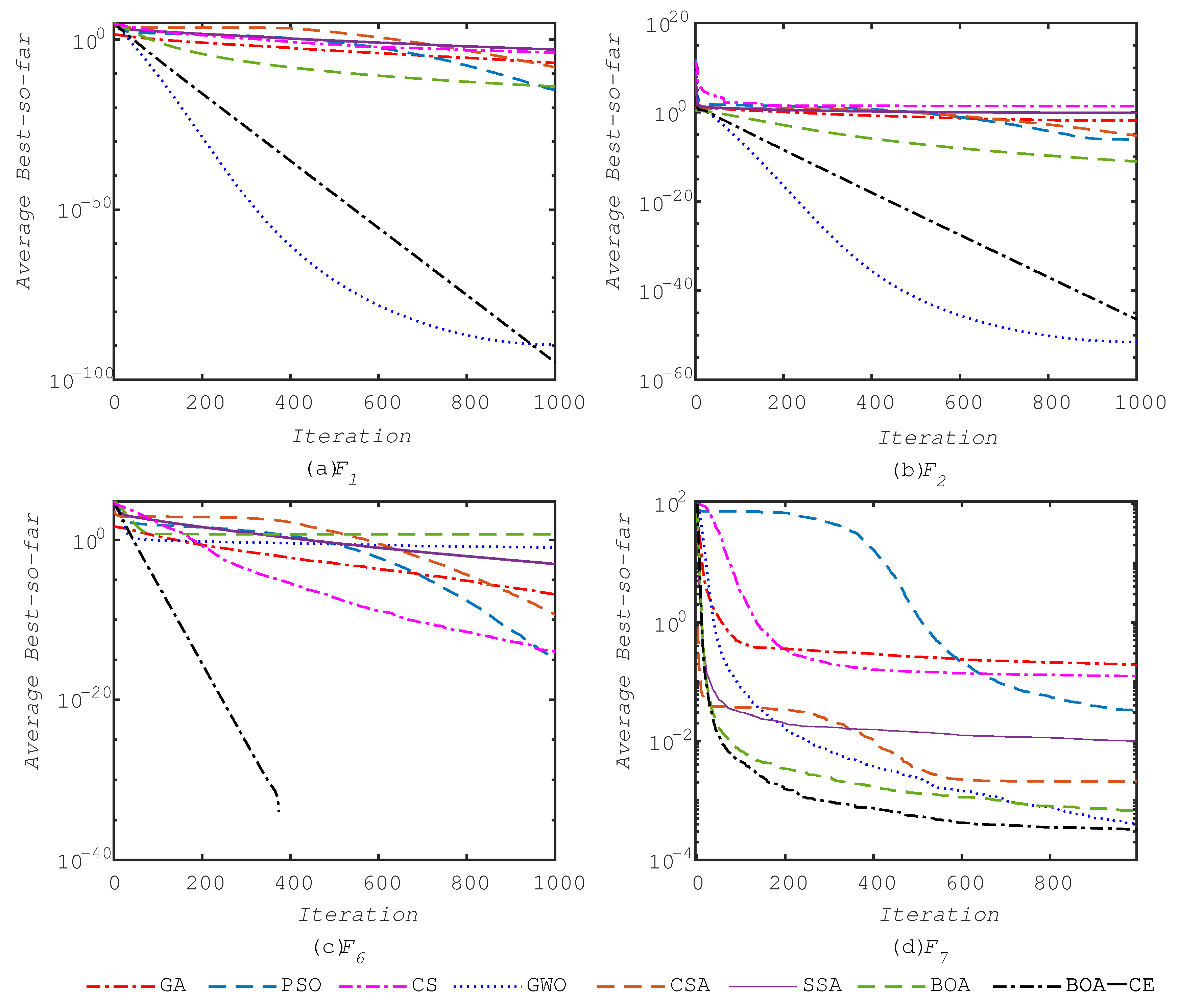
4.1. Results of the Algorithms Using Unimodal Test Functions

The results of the application of the algorithms to unimodal test functions are shown in Table 4. The best results are highlighted in bold. From Table 4, it can be found that: (1) the proposed method outperforms GA, PSO, BA, CSA, SSA, and BOA for the majority of the test functions; and (2) BOA-CE and GWO each provide the best results for three of these problems. This is due to the co-evolutionary technology that are adopted between the BOA and CE operators to enhance exploitation.
The progress of the average best value over 30 runs for some of the benchmark functions, such as F1, F2, F6, and F7, is illustrated in Figure 3. The figure clearly shows that the proposed BOA-CE algorithm rapidly converges towards the optimum and exploits it accurately. This benefit is mainly due to the algorithm’s excellent exploitation.

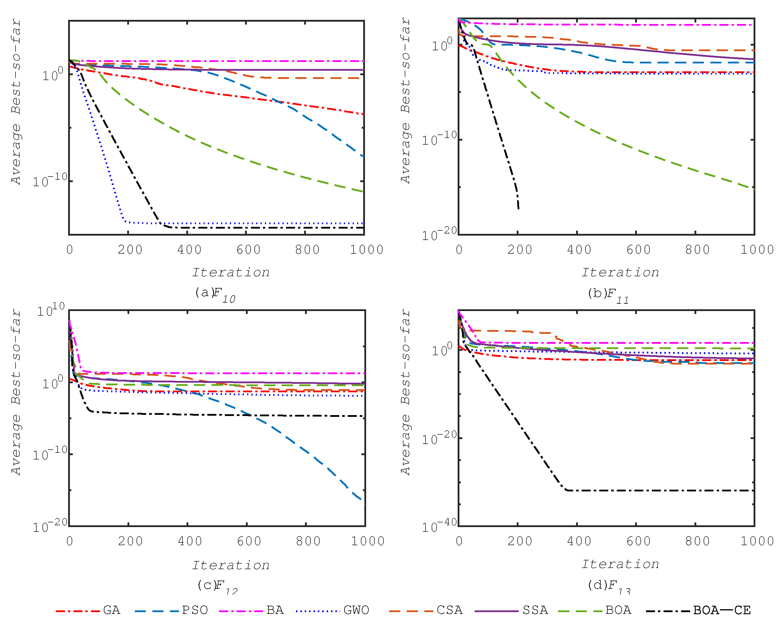
4.2. Results of the Algorithms Using Multimodal Test Functions

The results of the application of the algorithms to multimodal test functions are shown in Table 5. Table 5 shows that the BOA-CE method outperforms the other approaches in the majority of the test cases. Multimodal test functions are employed to benchmark the performance in terms of exploration and local optima avoidance. Therefore, these results prove that the BOA-CE algorithm has an excellent exploration which helps it to explore the promising regions of the search space. Additionally, the local optima avoidance of the improved method is also excellent, since it is able to avoid all of the local optima and find the global optimum for the majority of the multimodal test functions.
Figure 4 shows the convergence curves of the algorithms when applied to some of the multimodal test functions, such as F10, F11, F12, and F13. The figure shows that the BOA-CE algorithm has the fastest convergence for the majority of the multimodal test functions.

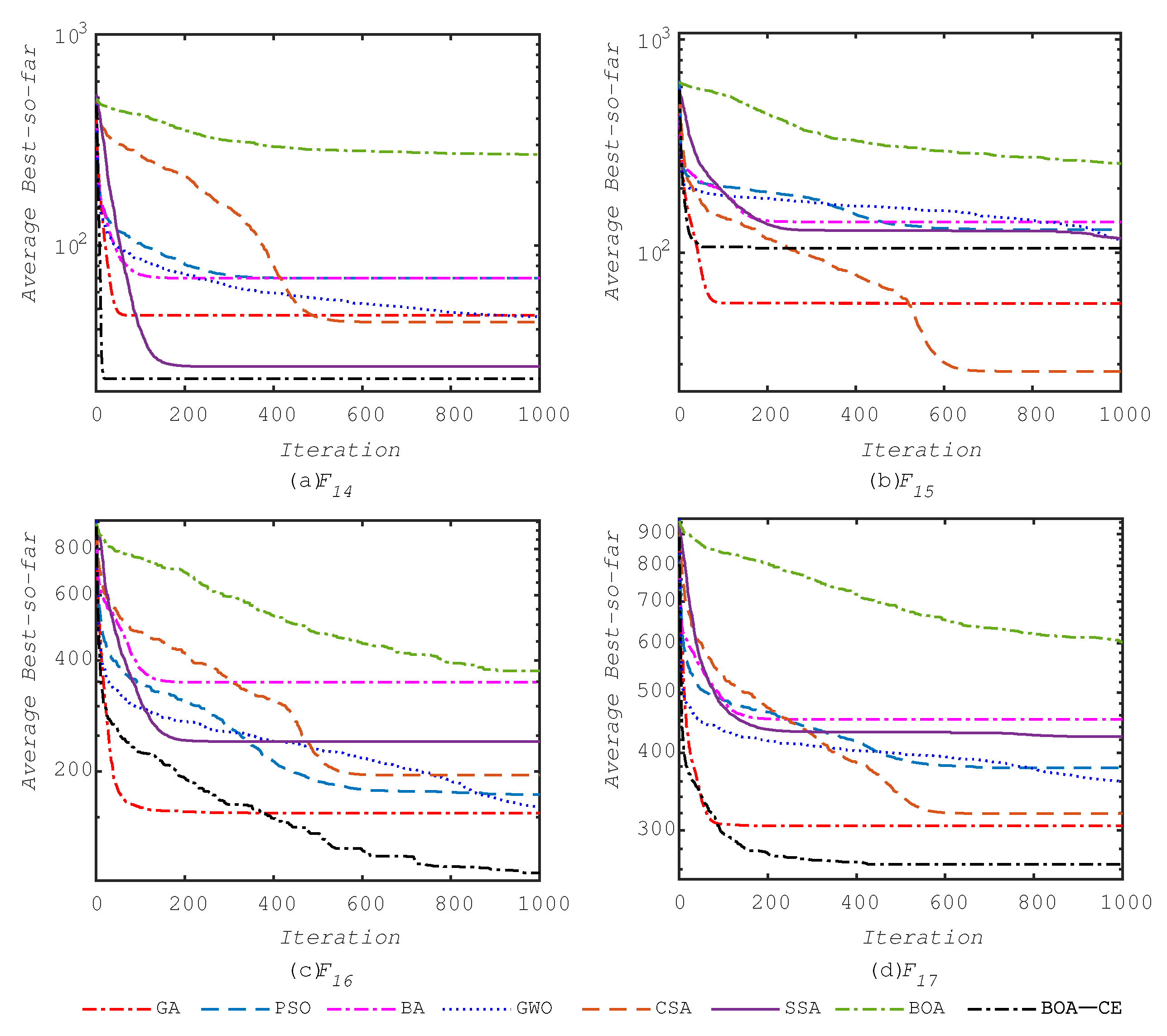
4.3. Results of the Algorithms on Composite Test Functions

The results of composite test functions are reported in Table 6. From Table 6, we can find that the BOA-CE algorithm outperforms others in most of the composite test functions. Considering the characteristics of composite test functions and these results, it may be stated that the BOA-CE algorithm appropriately balances exploration and exploitation to focus on the high-performance areas of the search space.
The convergence curves of the methods for some of the composite test functions are shown in Figure 5. Figure 5 clearly shows that the BOA-CE algorithm has the fastest convergence on the composite test functions.
In addition, Table 7 presents the time consumption of all the algorithms to solve the 19 benchmark functions. From Table 7, it can be seen that the least total time cost is PSO to solve all of the benchmark functions, followed by CSA, and the BOA-CE is ranked third, which is better than BOA.
The results of three test functions show that the local optima avoidance of the improved method was enhanced by embedding the cross-entropy method. This global stochastic optimization method enables the BOA-CE algorithm to achieve a proper balance between exploration and exploitation, and enhance its global search capability. Furthermore, the new method is particularly outstanding in solving multimodal function optimization problems.This provides a new method for solving complex engineering design optimization problems.

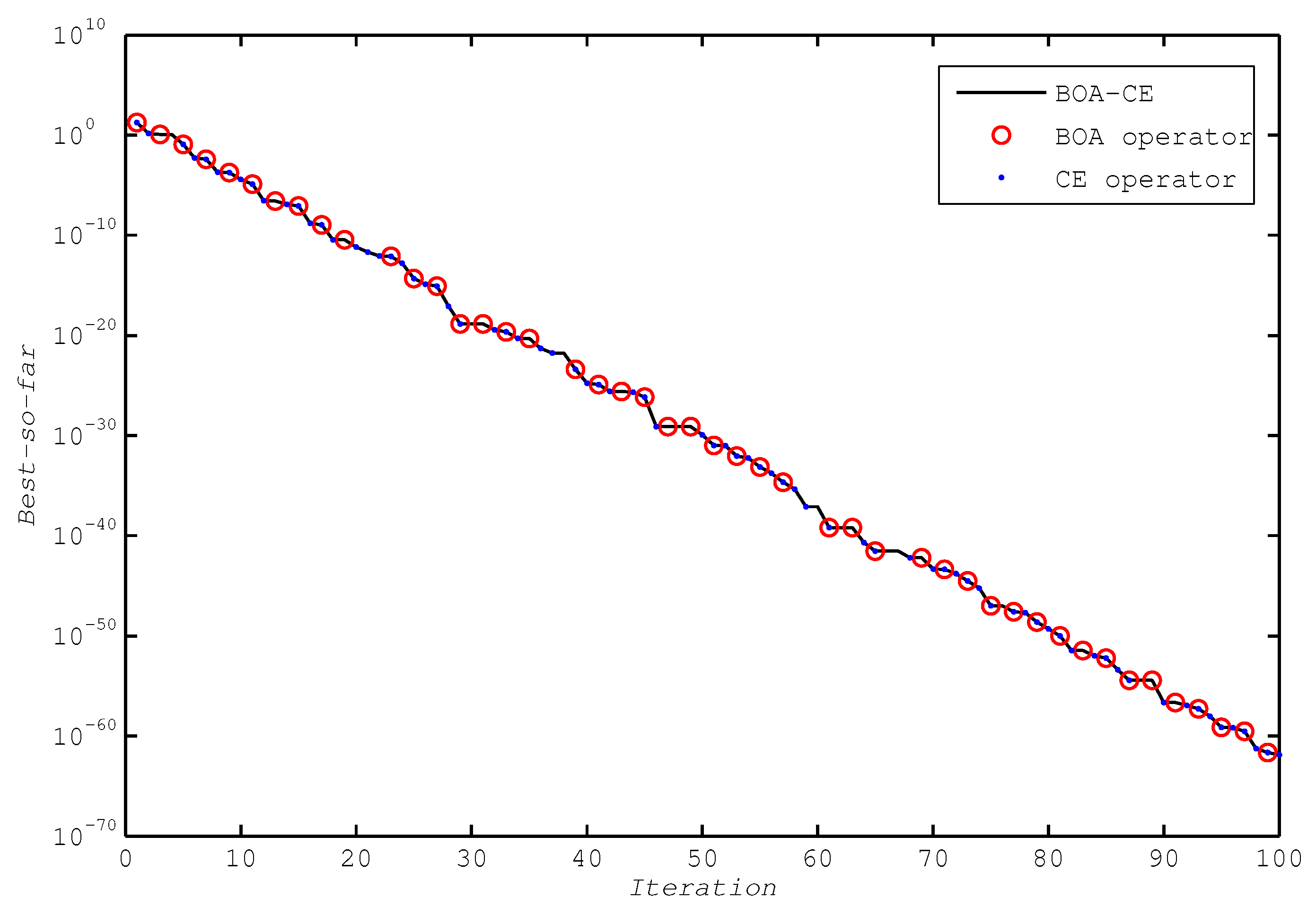
4.4. Analysis of the Hybrid BOA-CE Algorithm

The main reasons for the excellent performance of the proposed BOA-CE algorithm in solving global optimization problems may be stated as follows:
  • The BOA, which mimics the food foraging behavior of butterflies in nature, has the advantage of a fast convergence rate. Based on co-updating, the BOA-CE uses the excellent individuals obtained by the BOA operator to update the CE operator’s probability parameters during the iterative process, which speeds up the convergence rate of the CE operator.
  • The CE method is a global stochastic optimization method based on statistical model, and has the advantages of randomness, adaptability, and robustness, which bring a good population diversity to the BOA operator so that it can effectively avoid falling into a local optimum and improve its global search capability.
  • The BOA-CE algorithm employs a co-evolutionary technique to co-update the BOA operator’s population and the CE operator’s probability parameters. This enables the improved method to obtain an appropriate balance between exploration and exploitation and have more superior performance in terms of exploitation, exploration, and local optima avoidance when solving complex optimization problems.

5. Using the BOA-CE Algorithm for Classical Engineering Design Problems

In this section, the BOA-CE algorithm was tested on three classical constrained engineering design problems: a tension/compression spring, a welded beam, and a pressure vessel [9,15,19,20,28,31,47,48,49,50,51,52]. Constraint handling is a challenging task for a method when solving these problems. Penalty functions are divided into different types: static, dynamic, annealing, adaptive, co-evolutionary, and death penalty [47]. For the sake of simplicity, we equipped the BOA-CE algorithm with a death penalty function to handle constraints. Table 8 shows the BOA-CE parameters chosen to solve these design problems, where N is the population sizes of the BOA and CE operator, and I t e r m a x represents the maximum number of iterations.

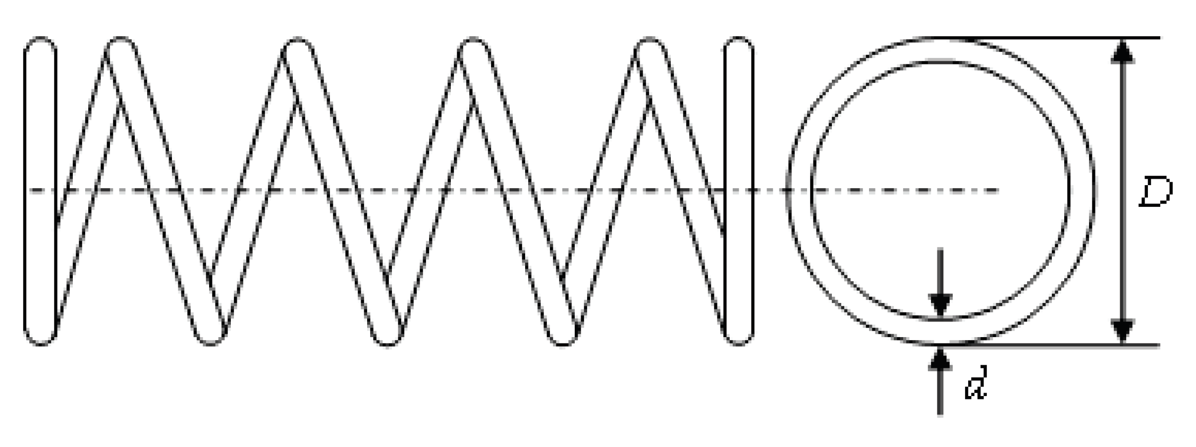
5.1. Tension/Compression Spring Design

The objective of this problem is to minimize the weight of the tension/compression spring shown in Figure 6. It contains three design variables: the wire diameter (d), mean coil diameter (D), and number of active coils (N), which are subject to one linear and three nonlinear inequality constraints on shear stress, surge frequency, and deflection. The optimization problem is formulated as follows:
min f ( x ) = ( x 3 + 2 ) x 2 x 1 2 ,
subject to
g 1 ( x ) = 1 x 2 3 x 3 71785 x 1 4 0 ,
g 2 ( x ) = 4 x 2 2 x 1 x 2 12566 ( x 2 x 1 3 x 1 4 ) + 1 5108 x 1 2 1 0 ,
g 3 ( x ) = 1 140.45 x 1 x 2 2 x 3 0 ,
g 4 ( x ) = x 1 + x 2 1.5 1 0 ,
where 0.05 x 1 2.00 , 0.25 x 2 1.30 , and 2.00 x 3 15.00 .
This problem has been popular among researchers and has been optimized using various meta-heuristic algorithms. To solve this problem, Coello employed GA [48], He and Wang employed PSO [49], Gandomi et al. used BA [50], Mirjalili employed GWO [15] and SSA [20], Lee and Geem [51] used HS, and Askarzadeh [19] used CSA. The best weight values are highlighted in bold. Table 9 shows a comparison of the results obtained using the BOA-CE algorithm and those obtained using the other algorithms. It can be seen that the BOA-CE and CSA algorithms find a design with the minimum weight for this problem and outperform all other algorithms.

5.2. Welded Beam Design

The objective of this problem is to minimize the fabrication cost of the welded beam shown in Figure 7. It contains four design variables: the thickness of the weld (h), length of the clamped bar (l), height of the bar (t), and thickness of the bar (b), which are subject to two linear and five nonlinear inequality constraints on shear stress, bending stress in the beam, buckling load, and end deflection of the beam. The optimization problem can be stated as follows:
min f ( x ) = 1.1047 x 1 2 x 2 + 0.04811 x 3 x 4 ( 14.0 + x 2 ) ,
subject to
g 1 ( x ) = τ ( x ) τ m a x 0 ,
g 2 ( x ) = σ ( x ) σ m a x 0 ,
g 3 ( x ) = δ ( x ) δ m a x 0 ,
g 4 ( x ) = x 1 x 4 0 ,
g 5 ( x ) = P P c ( x ) 0 ,
g 6 ( x ) = 0.125 x 1 0 ,
g 7 ( x ) = 1.10471 x 1 2 + 0.04811 x 3 x 4 ( 14.0 + x 2 ) 5.0 0 ,
where τ ( x ) = ( τ ) 2 + 2 τ τ x 2 2 R + ( τ ) 2 , τ = P 2 x 1 x 2 , τ = M R J , M = P ( L + x 2 2 ) , R = x 2 2 4 + ( x 1 + x 3 2 ) 2 , J = 2 { 2 x 1 x 2 [ x 2 2 4 + ( x 1 + x 3 2 ) 2 ] } , σ ( x ) = 6 P L x 4 x 3 2 , δ ( x ) = 6 P L 3 E x 3 3 x 4 , P c ( x ) = 4.013 E x 3 2 x 4 6 36 L 2 ( 1 x 3 2 L E 4 G ) , P = 6000 lb, L = 14 in, σ m a x = 0.25 in, E = 30 × 10 6 psi, G = 12 × 10 6 psi, τ m a x = 30,000 psi, 0.1 x 1 , x 4 2 , and 0.1 x 2 , x 3 10 .
The welded beam design problem has been tackled using many meta-heuristic algorithms, such as GA [48], PSO [49], BA [50], GWO [15], HS [51], WOA [18], and CSA [19]. The optimization results using the BOA-CE algorithm are compared with those from the literature in Table 10. The minimum cost is highlighted in bold. The table shows that BOA-CE outperforms all other algorithms except CSA, with only a slight difference in its result.

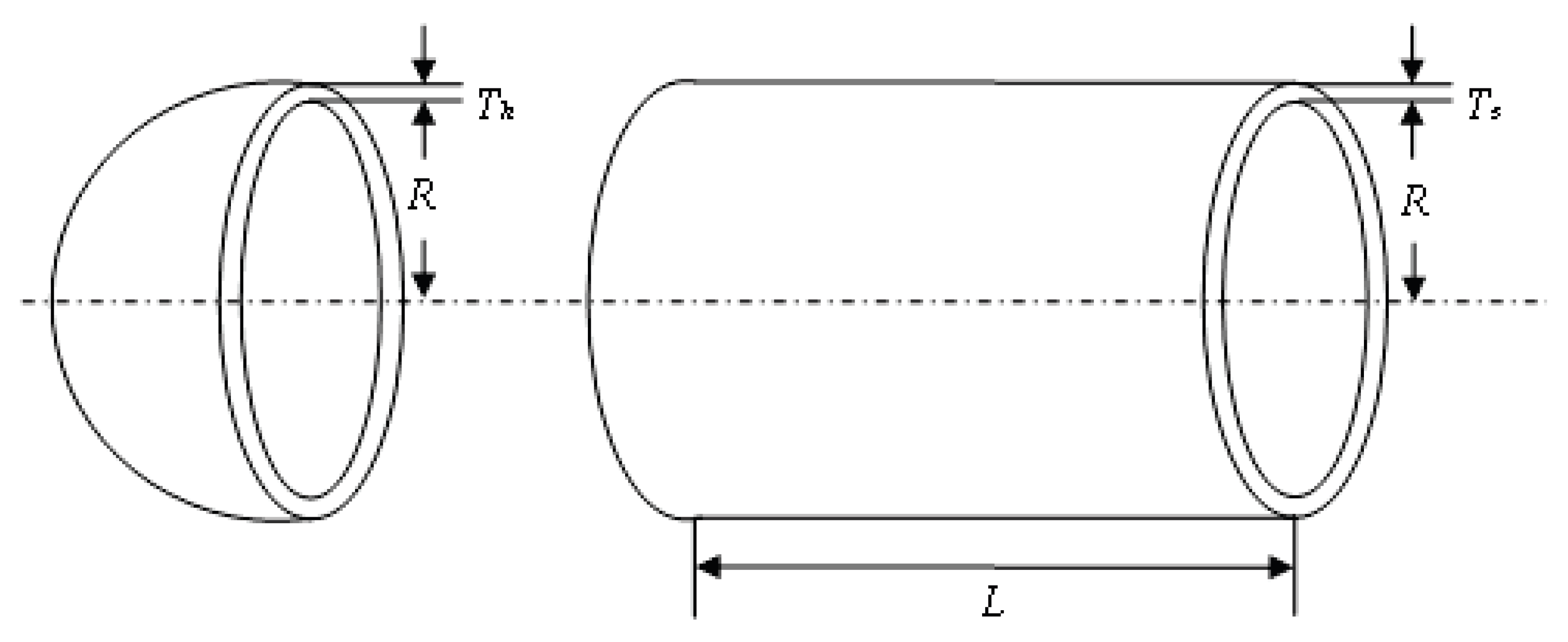
5.3. Pressure Vessel Design

The objective of this problem is to minimize the total cost of a pressure vessel considering the cost of material, forming and welding shown in Figure 8. There are two discrete and two continuous design variables: thickness of the shell ( T s ), thickness of the head ( T h ), inner radius (R) and length of the cylindrical section of the vessel (L), not including the head, which are subjected to three linear and one nonlinear inequality constraints. The thicknesses of the variables are integer multiples of 0.0625 inches. This optimization problem can be mathematically formulated as follows:
min f ( x ) = 0.6224 x 1 x 3 x 4 + 1.7781 x 2 x 3 2 + 3.1661 x 1 2 x 4 + 19.84 x 1 2 x 3 ,
subject to
g 1 ( x ) = x 1 + 0.0193 x 3 0 ,
g 2 ( x ) = x 3 + 0.00954 x 4 0 ,
g 3 ( x ) = π x 3 2 x 4 4 3 π x 3 3 + 1296000 0 ,
g 4 ( x ) = x 4 240 0 ,
where 0 < x 1 , x 2 99 , 0 < x 3 , x 4 200 .
In the past, this problem is solved by GA [48], PSO [49], BA [50], GWO [15], HS [51], WOA [18], and DE [52]. Table 11 shows optimization results of BOA-CE are compared with those found by other methods. It can be seen that BOA-CE and BA outperform all other algorithms except GWO. However the value of T h obtained by GWO is not an integer multiple of 0.0625 inches and thus does not satisfy the constraint.

6. Conclusions

In order to improve the global search ability of the BOA, an improved BOA algorithm, named BOA-CE, was constructed by embedding the CE method into the BOA using a co-evolutionary technique. A total of 19 test functions were used to evaluate the performance of the new method in terms of its exploration, exploitation, local optima avoidance, and convergence rate. The results of the test functions demonstrated that the proposed algorithm can effectively avoid falling into a local optima and has excellent local and global search capacity. This is mainly due to the co-evolutionary technique, which enables the new method to obtain an appropriate balance between exploration and exploitation and has more superior performance when solving complex function optimization problems. Furthermore, the paper also considered the solving of three classical engineering problems using the hybrid algorithm. The comparative results show that the BOA-CE algorithm provides very competitive results when solving real problems with unknown search spaces. In future research, a discrete version of the BOA-CE algorithm will be constructed to solve combinatorial optimization problems.

Author Contributions

G.L. designed the algorithm, implemented all experiments, and wrote the manuscript. F.S. revised the manuscript. P.Z. conducted the literature review and analyzed the data. C.L. revised the manuscript.

Funding

This research was funded by the National Natural Science Foundation of China (Grant No. 71761012), the Natural Science Foundation of Anhui Province (Grant No. 1808085MG224), and the Natural Science Foundation of West Anhui University (Grant No. WXZR201818).

Acknowledgments

The authors are grateful for the support provided by the Risk Management and Financial Engineering Lab at the University of Florida, Gainesville, FL 32611, USA.

Conflicts of Interest

The authors declare no conflict of interest.

Appendix A

Table A1. Mathematical formulation of the primitive functions in Table 3.
NameFormulation
Sphere f ( x ) = i = 1 D x i 2
Ackley f ( x ) = 20 exp ( 0.2 1 D i = 1 D x i 2 ) exp ( 1 D i = 1 D cos ( 2 π x i ) ) + 20 + e
Griewank f ( x ) = 1 4000 i = 1 D x i 2 i = 1 D cos ( x i i ) + 1
Weierstrass f ( x ) = i = 1 D ( k = 0 k m a x [ a k cos ( 2 π b k ( x i + 0.5 ) ) ] ) D k = 0 k m a x [ a k cos ( 2 π b k · 0.5 ) ] , a = 0.5 , b = 3 , k m a x = 20
Rastrigin f ( x ) = i = 1 D 1 [ x i 2 10 cos ( 2 π x i ) + 10 ]
D: dimensions.

References

  1. Hu, X.; Eberhart, R.C.; Shi, Y. Engineering optimization with particle swarm. In Proceedings of the 2003 IEEE Swarm Intelligence Symposium, Indianapolis, IN, USA, 26–26 April 2003; pp. 53–57. [Google Scholar]
  2. Sergeyev, Y.D.; Kvasov, D.E. A deterministic global optimization using smooth diagonal auxiliary functions. Commun. Nonlinear Sci. Numer. Simul. 2015, 21, 99–111. [Google Scholar] [CrossRef]
  3. Lera, D.; Sergeyev, Y.D. GOSH: Derivative-free global optimization using multi-dimensional space-filling curves. J. Glob. Optim. 2018, 71, 193–211. [Google Scholar] [CrossRef]
  4. Sergeyev, Y.D.; Kvasov, D.E.; Mukhametzhanov, M.S. On the efficiency of nature-inspired metaheuristics in expensive global optimization with limited budget. Sci. Rep. 2018, 8, 453. [Google Scholar] [CrossRef] [PubMed]
  5. Zilinskas, A.; Zhigljavsky, A. Stochastic Global Optimization: A Review on the Occasion of 25 Years of Informatica. Informatica 2016, 27, 229–256. [Google Scholar] [CrossRef]
  6. Goldfeld, S.M.; Quandt, R.E.; Trotter, H.F. Maximization by quadratic hill-climbing. Econometrica 1966, 34, 541–551. [Google Scholar] [CrossRef]
  7. Abbasbandy, S. Improving Newton–Raphson method for nonlinear equations by modified Adomian decomposition method. Appl. Math. Comput. 2003, 145, 887–893. [Google Scholar] [CrossRef]
  8. Jones, D.R.; Perttunen, C.D.; Stuckman, B.E. Lipschitzian optimization without the Lipschitz constant. J. Optim. Theory Appl. 1993, 79, 157–181. [Google Scholar] [CrossRef]
  9. Mirjalili, S. The Ant Lion Optimizer. Adv. Eng. Softw. 2015, 83, 80–98. [Google Scholar] [CrossRef]
  10. Whitley, D. A genetic algorithm tutorial. Stat. Comput. 1994, 4, 65–85. [Google Scholar] [CrossRef]
  11. Wieczorek, L.; Ignaciuk, P. Continuous Genetic Algorithms as Intelligent Assistance for Resource Distribution in Logistic Systems. Data 2018, 3, 68. [Google Scholar] [CrossRef]
  12. Kennedy, J.; Eberhart, R.C. Particle swarm optimization. In Proceedings of the 1995 IEEE International Conference on Neural Networks, Perth, Australia, 27 November–1 December 1995; pp. 1942–1948. [Google Scholar]
  13. Yang, X.S.; Deb, S. Engineering Optimisation by Cuckoo Search. Int. J. Math. Model. Numer. Optim. 2010, 1, 330–343. [Google Scholar] [CrossRef]
  14. Yang, X.S. A new metaheuristic bat-inspired algorithm. In Nature Inspired Cooperative Strategies for Optimization (NICSO 2010); Springer: Berlin/Heidelberg, Germany, 2010; pp. 65–74. [Google Scholar]
  15. Mirjalili, S.; Mirjalili, S.M.; Lewis, A. Grey Wolf Optimizer. Adv. Eng. Softw. 2014, 69, 46–61. [Google Scholar] [CrossRef] [Green Version]
  16. Ghaemi, M.; Feizi-Derakhshi, M.R. Forest Optimization Algorithm. Expert Syst. Appl. 2014, 41, 6676–6687. [Google Scholar] [CrossRef]
  17. Naz, M.; Zafar, K.; Khan, A. Ensemble Based Classification of Sentiments Using Forest Optimization Algorithm. Data 2019, 4, 76. [Google Scholar] [CrossRef]
  18. Mirjalili, S.; Lewis, A. The Whale Optimization Algorithm. Adv. Eng. Softw. 2016, 95, 51–67. [Google Scholar] [CrossRef]
  19. Askarzadeh, A. A novel metaheuristic method for solving constrained engineering optimization problems: Crow search algorithm. Comput. Struct. 2016, 169, 1–12. [Google Scholar] [CrossRef]
  20. Mirjalili, S.; Gandomi, A.H.; Mirjalili, S.Z.; Saremi, S.; Faris, H.; Mirjalili, S.M. Salp Swarm Algorithm: A bio-inspired optimizer for engineering design problems. Adv. Eng. Softw. 2017, 114, 163–191. [Google Scholar] [CrossRef]
  21. Arora, S.; Singh, S. Butterfly algorithm with Lèvy Flights for global optimization. In Proceedings of the 2015 International Conference on Signal Processing, Computing and Control (ISPCC), Waknaghat, India, 24–26 September 2015; pp. 220–224. [Google Scholar]
  22. Arora, S.; Singh, S. Butterfly optimization algorithm: A novel approach for global optimization. Soft Comput. 2019, 23, 715–734. [Google Scholar] [CrossRef]
  23. Yang, X.S.; Deb, S. Cuckoo search: Recent advances and applications. Neural Comput. Appl. 2014, 24, 169–174. [Google Scholar] [CrossRef]
  24. Wolpert, D.H.; Macready, W.G. No Free Lunch Theorems for Optimization. IEEE Trans. Evol. Comput. 1997, 1, 67–82. [Google Scholar] [CrossRef]
  25. Lai, X.S.; Zhang, M.Y. An Efficient Ensemble of GA and PSO for Real Function Optimization. In Proceedings of the 2009 2nd IEEE International Conference on Computer Science and Information Technology, Beijing, China, 8–11 August 2009; pp. 651–655. [Google Scholar]
  26. Mirjalili, S.; Hashim, S.Z.M. A New Hybrid PSOGSA Algorithm for Function Optimization. In Proceedings of the 2010 International Conference on Computer and Information Application (2010 ICCIA), Tianjin, China, 3–5 December 2010; pp. 374–377. [Google Scholar]
  27. Abdullah, A.; Deris, S.; Mohamad, M.S.; Hashim, S.Z.M. A New Hybrid Firefly Algorithm for Complex and Nonlinear Problem. In Distributed Computing and Artificial Intelligence; Springer: Berlin/Heidelberg, Germany, 2012; pp. 673–680. [Google Scholar] [Green Version]
  28. He, X.S.; Ding, W.J.; Yang, X.S. Bat algorithm based on simulated annealing and Gaussian perturbations. Neural Comput. Appl. 2014, 25, 459–468. [Google Scholar] [CrossRef]
  29. Mafarja, M.M.; Mirjalili, S. Hybrid Whale Optimization Algorithm with simulated annealing for feature selection. Neurocomputing 2017, 260, 302–312. [Google Scholar] [CrossRef]
  30. Pepelyshev, P.; Zhigljavsky, A.; Zilinskas, A. Performance of global random search algorithms for large dimensions. J. Glob. Optim. 2018, 71, 57–71. [Google Scholar] [CrossRef]
  31. Rubinstein, R.Y. Optimization of Computer Simulation Models with Rare Events. Eur. J. Oper. Res. 1997, 99, 89–112. [Google Scholar] [CrossRef]
  32. Arora, S.; Singh, S. An Improved Butterfly Optimization Algorithm for Global Optimization. Adv. Sci. 2017, 8, 711–717. [Google Scholar] [CrossRef]
  33. Arora, S.; Singh, S. Node Localization in Wireless Sensor Networks Using Butterfly Optimization Algorithm. Arab. J. Sci. Eng. 2017, 42, 3325–3335. [Google Scholar] [CrossRef]
  34. Kroese, D.P.; Portsky, S.; Rubinstein, R.Y. The Cross-Entropy Method for Continuous Multi-extremal Optimization. Methodol. Comput. Appl. Probab. 2006, 8, 383–407. [Google Scholar] [CrossRef]
  35. Bekker, J.; Aldrich, C. The cross-entropy method in multi-objective optimisation: An assessment. Eur. J. Oper. Res. 2011, 211, 112–121. [Google Scholar] [CrossRef]
  36. Rubinstein, R.Y. The Cross-Entropy Method for Combinatorial and Continuous Optimization. Methodol. Comput. Appl. Probab. 1999, 1, 127–190. [Google Scholar] [CrossRef]
  37. Rubinstein, R.Y.; Kroese, D.P. The Cross-Entropy Method: A Unified Approach to Combinatorial Optimization, Monte Carlo Simulation and Machine Learning; Springer: New York, NY, USA, 2004. [Google Scholar]
  38. Chepuri, K.; Homem-De-Mello, T. Solving the vehicle routing problem with stochastic demands using the cross-entropy method. Ann. Oper. Res. 2005, 134, 153–181. [Google Scholar] [CrossRef]
  39. Yu, J.; Konaka, S.; Akutagawa, M.; Zhang, Q. Cross-Entropy-Based Energy-Efficient Radio Resource Management in HetNets with Coordinated Multiple Points. Information 2016, 7, 3. [Google Scholar] [CrossRef]
  40. Joseph, A.G.; Bhatnagar, S. An online prediction algorithm for reinforcement learning with linear function approximation using cross entropy method. Mach. Learn. 2018, 107, 1385–1429. [Google Scholar] [CrossRef] [Green Version]
  41. Peherstorfer, B.; Kramer, B.; Willcox, K. Multifidelity preconditioning of the cross-entropy method for rare event simulation and failure probability estimation. SIAM/ASA J. Uncertain. Quantif. 2018, 6, 737–761. [Google Scholar] [CrossRef]
  42. Wang, Y.; Yang, H.; Qin, K. The Consistency between Cross-Entropy and Distance Measures in Fuzzy Sets. Symmetry 2019, 11, 386. [Google Scholar] [CrossRef]
  43. Pramanik, S.; Dalapati, S.; Alam, S.; Smarandache, F.; Roy, T.K. NS-Cross Entropy-Based MAGDM under Single-Valued Neutrosophic Set Environment. Information 2018, 9, 37. [Google Scholar] [CrossRef]
  44. Eiben, A.E.; Schipper, C.A. On evolutionary exploration and exploitation. Fund. Inform. 1998, 35, 35–50. [Google Scholar]
  45. Yao, X.; Liu, Y.; Lin, G.M. Evolutionary Programming Made Faster. IEEE Trans. Evol. Comput. 1999, 3, 82–102. [Google Scholar]
  46. Liang, J.; Suganthan, P.; Deb, K. Novel composition test functions for numerical global optimization. In Proceedings of the 2005 IEEE Swarm Intelligence Symposium, Pasadena, CA, USA, 8–10 June 2005; pp. 68–75. [Google Scholar]
  47. Coello, C.C.A.; Mezura, M.E. Constraint-handling in genetic algorithms through the use of dominance-based tournament selection. Adv. Eng. Inform. 2002, 16, 193–203. [Google Scholar] [CrossRef]
  48. Coello, C.C.A. Use of a Self-Adaptive Penalty Approach for Engineering Optimization Problems. Comput. Ind. 2000, 41, 113–127. [Google Scholar] [CrossRef]
  49. He, Q.; Wang, L. An effective co-evolutionary particle swarm optimization for constrained engineering design problems. Eng. Appl. Artif. Intell. 2007, 20, 89–99. [Google Scholar] [CrossRef]
  50. Gandomi, A.H.; Yang, X.S.; Alavi, A.H.; Talatahari, S. Bat algorithm for constrained optimization tasks. Neural Comput. Appl. 2013, 22, 1239–1255. [Google Scholar] [CrossRef]
  51. Lee, K.S.; Geem, Z.W. A new meta-heuristic algorithm for continuous engineering optimization: Harmony search theory and practice. Comput. Methods Appl. Mech. Eng. 2005, 194, 3902–3933. [Google Scholar] [CrossRef]
  52. Huang, F.; Wang, L.; He, Q. An effective co-evolutionary differential evolution for constrained optimization. Appl. Math. Comput. 2007, 186, 340–356. [Google Scholar] [CrossRef]
Figure 1. The flow chart of the BOA-CE algorithm.
Symmetry 11 01049 g001
Figure 2. The BOA operator and CE operator co-update the current best f of the 2D Sphere function.
Symmetry 11 01049 g002
Figure 3. Convergence of algorithms when applied to some unimodal benchmark functions.
Symmetry 11 01049 g003
Figure 4. Convergence of algorithms on some unimodal benchmark functions.
Symmetry 11 01049 g004
Figure 5. Convergence of algorithms when applied to some composite benchmark functions.
Symmetry 11 01049 g005
Figure 6. The tension/compression spring design problem.
Symmetry 11 01049 g006
Figure 7. The welded beam design problem.
Symmetry 11 01049 g007
Figure 8. The tension/compression spring design problem.
Symmetry 11 01049 g008
Table 1. Unimodal benchmark functions.
FunctionDimRange F min
F 1 ( x ) = i = 1 n x i 2 30 [ 100 , 100 ] 0
F 2 ( x ) = i = 1 n x i + i = 1 n x i 30 [ 10 , 10 ] 0
F 3 ( x ) = i = 1 n ( j = 1 i x j ) 2 30 [ 100 , 100 ] 0
F 4 ( x ) = max i { x i , 1 i n } 30 [ 100 , 100 ] 0
F 5 ( x ) = i = 1 n 1 [ 100 ( x i + 1 x i 2 ) 2 + ( x i 1 ) 2 ] 30 [ 30 , 30 ] 0
F 6 ( x ) = i = 1 n ( [ x i + 0.5 ] ) 2 30 [ 100 , 100 ] 0
F 7 ( x ) = i = 1 n i x i 4 + r a n d o m [ 0 , 1 ) 30 [ 1.28 , 1.28 ] 0
Table 2. Multi-modal benchmark functions.
FunctionDimRange F min
F 8 ( x ) = i = 1 n x i sin ( x i ) 30 [ 500 , 500 ] 12,569.487
F 9 ( x ) = i = 1 n 1 [ x i 2 10 cos ( 2 π x i ) + 10 ] 30 [ 5.12 , 5.12 ] 0
F 10 ( x ) = 20 exp ( 0.2 1 n i = 1 n x i 2 ) exp ( 1 n i = 1 n cos ( 2 π x i ) ) 30[−32, 32]0
+ 20 + e
F 11 ( x ) = 1 4000 i = 1 n x i 2 i = 1 n cos ( x i i ) + 1 30[−600, 600]0
F 12 ( x ) = π n { 10 sin 2 ( π y 1 ) + i = 1 n 1 ( y i 1 ) 2 [ 1 + 10 sin 2 ( π y i + 1 ) 30[−50, 50]0
+ ( y n + 1 ) 2 ] } + i = 1 n u ( x i , 10 , 100 , 4 )
y i = 1 + x i + 1 4
u ( x i , a , k , m ) = k ( x i a ) m , x i > a 0 , a x i a k ( x i a ) m , x i < a
F 13 ( x ) = 0.1 { sin 2 ( 3 π x 1 ) + i = 1 n ( x i 1 ) 2 [ 1 + sin 2 ( 3 π x i + 1 ) ] } 30[−50, 50]0
+ i = 1 n u ( x i , 5 , 100 , 4 )
Table 3. Composite benchmark functions.
Function 1 DimRange F min
F 14 (CF1)
f 1 , f 2 , , f 10 = Sphere Function,10 [ 5 , 5 ] 0
[ λ 1 , λ 2 , , λ 10 ] = [ 1 , 1 , , 1 ] , [ σ 1 , σ 2 , , σ 10 ] = [ 1 / 100 , 5 / 100 , , 5 / 100 ]
F 15 (CF2)
f 1 , f 2 , , f 10 = Griewank’s Function,10 [ 5 , 5 ] 0
[ λ 1 , λ 2 , , λ 10 ] = [ 1 , 1 , , 1 ] , [ σ 1 , σ 2 , , σ 10 ] = [ 1 / 100 , 5 / 100 , , 5 / 100 ]
F 16 (CF3)
f 1 , f 2 , , f 10 = Griewank’s Function,10 [ 5 , 5 ] 0
[ λ 1 , λ 2 , , λ 10 ] = [ 1 , 1 , , 1 ] , [ σ 1 , σ 2 , , σ 10 ] = [ 1 , 1 , , 1 ]
F 17 (CF4)
f 1 , f 2 = Ackley’s Function, f 3 , f 4 = Rastrigin’s Function,
f 5 , f 6 = Weierstrass Function, f 7 , f 8 = Griewank’s Function,10 [ 5 , 5 ] 0
f 9 , f 10 = Sphere Function, [ λ 1 , λ 2 , , λ 10 ] = [ 1 , 1 , , 1 ] ,
[ σ 1 , σ 2 , , σ 10 ] = [ 5 32 , 5 32 , 1 , 1 , 5 0.5 , 5 0.5 , 5 100 , 5 100 , 5 100 , 5 100 ]
F 18 (CF5)
f 1 , f 2 = Rastrigin’s Function, f 3 , f 4 = Weierstrass Function,
f 5 , f 6 = Griewank’s Function, f 7 , f 8 = Ackley’sGriewank’s Function,10 [ 5 , 5 ] 0
f 9 , f 10 = Sphere Function, [ λ 1 , λ 2 , , λ 10 ] = [ 1 , 1 , , 1 ] ,
[ σ 1 , σ 2 , , σ 10 ] = [ 1 5 , 1 5 , 5 0.5 , 5 0.5 , 5 100 , 5 100 , 5 32 , 5 32 , 5 100 , 5 100 ]
F 19 (CF6)
f 1 , f 2 = Rastrigin’s Function, f 3 , f 4 = Weierstrass Function,
f 5 , f 6 = Griewank’s Function, f 7 , f 8 = Ackley’sGriewank’s Function,
f 9 , f 10 = Sphere Function, [ λ 1 , λ 2 , , λ 10 ] = [ 1 , 1 , , 1 ] ,10 [ 5 , 5 ] 0
[ λ 1 , λ 2 , , λ 10 ] = [ 0.1 , 0.2 , 0.3 , 0.4 , 0.5 , 0.6 , 0.7 , 0.8 , 0.9 , 1 ] ,
[ σ 1 , σ 2 , , σ 10 ] = [ 0.1 × 1 5 , 0.2 × 1 5 , 0.3 × 0.4 × 5 0.5 , 0.5 × 5 0.5 ,
0.6 × 5 100 , 0.7 × 5 100 , 0.8 × 5 32 , 0.9 × 5 32 , 1 × 5 100 , 5 100 ]
1 Mathematical formulation of Sphere, Ackley, Rastrigin, Weierstrass, and Griewank can be found in Appendix A Table A1.
Table 4. Results of unimodal benchmark functions.
Fun.Metr.GAPSOBAGWOCSASSABOABOA-CE
F1Mean 1.44 × 10 07 1.43 × 10 15 1.46 × 10 04 1.97 × 10 90 1.20 × 10 03 6.70 × 10 09 1.57 × 10 14 1.26 × 10 95
SD 4.32 × 10 07 3.42 × 10 15 7.98 × 10 04 5.36 × 10 90 5.64 × 10 04 1.23 × 10 09 7.69 × 10 16 9.78 × 10 96
F2Mean 1.48 × 10 02 7.50 × 10 07 2.57 × 10 + 01 2.92 × 10 52 7.16 × 10 01 6.00 × 10 06 9.14 × 10 12 3.60 × 10 47
SD 6.05 × 10 02 3.30 × 10 06 3.93 × 10 + 01 3.35 × 10 52 4.51 × 10 01 1.33 × 10 06 1.37 × 10 12 2.50 × 10 47
F3Mean 5.20 × 10 01 2.30 × 10 + 00 2.42 × 10 + 03 1.74 × 10 26 8.30 × 10 + 00 8.33 × 10 10 1.60 × 10 14 2.44 × 10 09
SD 1.95 × 10 01 1.18 × 10 + 00 2.18 × 10 + 03 5.09 × 10 26 4.74 × 10 + 00 3.05 × 10 10 9.73 × 10 16 1.83 × 10 10
F4Mean 1.88 × 10 01 2.01 × 10 01 3.56 × 10 + 01 1.74 × 10 21 1.35 × 10 + 00 1.23 × 10 05 1.09 × 10 11 8.82 × 10 07
SD 4.63 × 10 01 6.33 × 10 02 6.27 × 10 13 2.81 × 10 21 6.84 × 10 01 1.99 × 10 06 6.72 × 10 13 1.51 × 10 07
F5Mean 1.87 × 10 + 01 4.28 × 10 + 01 1.47 × 10 + 02 2.62 × 10 + 01 4.19 × 10 + 01 1.26 × 10 + 01 2.89 × 10 + 01 2.79 × 10 + 01
SD 2.82 × 10 + 01 3.07 × 10 + 01 2.71 × 10 + 02 6.30 × 10 01 2.82 × 10 + 01 2.86 × 10 + 01 3.95 × 10 02 2.56 × 10 01
F6Mean 1.56 × 10 07 1.47 × 10 15 1.06 × 10 14 1.10 × 10 01 9.65 × 10 04 4.74 × 10 10 5.05 × 10 + 00 0
SD 2.37 × 10 07 2.20 × 10 15 5.40 × 10 14 1.58 × 10 01 4.19 × 10 04 1.44 × 10 10 5.34 × 10 01 0
F7Mean 3.79 × 10 01 3.22 × 10 02 1.25 × 10 01 3.99 × 10 04 9.87 × 10 03 2.06 × 10 03 6.68 × 10 04 3.29 × 10 04
SD 9.79 × 10 02 1.12 × 10 02 4.30 × 10 02 1.65 × 10 04 4.50 × 10 03 1.22 × 10 03 3.25 × 10 04 1.52 × 10 04
Table 5. Results of multi-modal benchmark functions.
Fun.Metr.GAPSOBAGWOCSASSABOABOA-CE
F8Mean 10,486.64 6500.75 3525.02 6941.03 7294.61 2824.35 4246.74 4017.15
SD 626.18 819.29 192.65 641.14 801.93 211.32 350.36 323.25
F9Mean 1.33 × 10 + 00 3.24 × 10 01 1.35 × 10 + 02 3.45 × 10 + 01 1.87 × 10 + 01 1.21 × 10 + 01 3.03 × 10 14 1.01 × 10 + 01
SD 1.23 × 10 + 00 1.78 × 10 + 00 3.38 × 10 + 01 1.14 × 10 + 01 7.82 × 10 + 00 5.86 × 10 + 00 1.46 × 10 13 3.46 × 10 + 01
F10Mean 1.76 × 10 04 1.10 × 10 14 1.64 × 10 + 01 1.89 × 10 08 2.56 × 10 + 00 4.24 × 10 01 1.01 × 10 11 4.44 × 10 15
SD 7.59 × 10 05 3.11 × 10 15 2.30 × 10 + 00 1.72 × 10 08 6.99 × 10 01 6.81 × 10 01 1.10 × 10 12 0
F11Mean 1.23 × 10 03 8.70 × 10 04 1.22 × 10 + 02 1.29 × 10 02 2.89 × 10 02 2.47 × 10 01 5.59 × 10 16 0
SD 3.41 × 10 03 2.68 × 10 03 5.54 × 10 + 01 1.45 × 10 02 1.34 × 10 02 1.46 × 10 01 5.64 × 10 16 0
F12Mean 5.19 × 10 02 1.35 × 10 02 1.82 × 10 + 01 9.96 × 10 18 6.25 × 10 01 8.53 × 10 02 3.84 × 10 01 2.02 × 10 05
SD 1.12 × 10 01 9.37 × 10 03 5.84 × 10 + 00 1.13 × 10 17 5.39 × 10 01 2.11 × 10 01 1.13 × 10 01 8.76 × 10 05
F13Mean 5.09 × 10 03 1.51 × 10 01 3.85 × 10 + 01 1.10 × 10 03 1.20 × 10 02 7.32 × 10 04 2.24 × 10 + 00 1.35 × 10 32
SD 1.23 × 10 02 1.43 × 10 01 1.62 × 10 + 01 3.35 × 10 03 1.51 × 10 02 2.79 × 10 030 4.04 × 10 01 5.57 × 10 48
Table 6. Results of composite benchmark functions.
Fun.Metr.GAPSOBAGWOCSASSABOABOA-CE
F14Mean 46.67 70.00 70.00 45.90 26.67 43.33 270.28 23.33
SD 50.74 95.23 83.67 71.84 44.98 67.89 58.82 43.02
F15Mean 57.91 128.09 139.61 115.17 116.59 27.77 262.27 104.76
SD 62.53 76.97 95.29 82.14 61.98 17.39 110.66 72.26
F16Mean 154.18 172.96 348.41 160.34 240.86 195.18 374.19 105.92
SD 42.63 75.64 111.53 48.84 66.57 38.64 57.17 59.17
F17Mean 305.43 378.64 452.73 360.09 424.94 319.45 602.76 264.51
SD 35.95 128.17 114.34 105.96 92.62 27.58 85.08 96.10
F18Mean 53.09 92.41 85.22 56.75 9.49 14.10 130.84 71.00
SD 79.02 136.96 150.90 62.29 17.69 29.53 59.39 47.42
F19Mean 627.64 765.17 745.07 698.91 497.13 55.26 819.40 790.79
SD 192.16 191.11 198.03 201.69 17.93 152.72 112.13 153.62
Table 7. Time consumption of BOA-CE solving 19 benchmark functions.
Fun.GAPSOBAGWOCSASSABOABOA-CE
F18.960.200.330.550.100.660.460.41
F28.800.210.350.570.110.430.490.42
F310.750.762.521.132.020.561.611.15
F48.440.200.410.550.140.380.460.40
F59.110.270.590.620.290.450.590.51
F68.570.200.340.550.100.380.450.40
F79.290.540.911.140.580.520.840.90
F88.720.310.870.650.190.440.680.62
F98.810.260.410.570.150.400.580.48
F108.660.260.430.590.170.410.550.45
F118.970.310.690.640.340.470.660.54
F1210.141.171.621.521.160.912.451.67
F1310.101.171.621.521.170.912.461.66
F14264.89249.55256.03304.78260.24266.09263.94265.80
F15261.13232.07261.98300.36258.01255.73263.67259.32
F16259.28210.24269.61250.40263.24258.70259.05252.60
F17313.15212.06287.05273.28282.19283.91286.06282.38
F18293.31262.41289.38272.57286.17286.81288.63286.88
F19287.42172.65278.74288.92282.58297.25291.06284.31
Total1798.501344.821653.881700.911638.951655.411664.701640.89
Ranking81572643
Table 8. Parameters of the BOA-CE algorithm for solving design problems.
Design ProblemBOA OperatorCE Operator
N Iter max N Iter max
Tension/compression spring1005010050
Welded beam10010010050
Pressure vessel10010010050
Table 9. A comparison of results for the tension/compression spring design problem.
AlgorithmOptimum VariablesOptimum Weight
d D N
GA [48]0.0514800.35166111.6322010.0127048
PSO [49]0.0517280.35764411.2445430.012675
BA [50]0.0516900.35673011.2885000.012670
GWO [15]0.0516900.35673711.2888500.012666
HS [51]0.0511540.34987112.0764320.012671
CSA [19]0.0516890.35671711.2890120.012665
SSA [20]0.0512070.34521512.0040320.012676
BOA-CE0.0516180.35500411.3901440.012665
Table 10. A comparison of results for the tension/compression spring design problem.
AlgorithmOptimum VariablesOptimum Cost
h l t b
GA [48]0.2059863.4713289.0202240.2064801.728226
PSO [49]0.2023693.5442149.0482100.2057231.731485
BA [50]0.20153.5629.04140.20571.7312
GWO [15]0.2056763.4783779.036810.2057781.72624
HS [51]0.24426.22318.29150.24432.3807
WOA [18]0.2053963.4842939.0374260.2062761.730499
CSA [19]0.2057303.4704899.0366240.2057301.724852
BOA-CE0.2057303.4704819.0366110.2057301.724854
Table 11. A comparison of results for the tension/compression spring design problem.
AlgorithmOptimum VariablesOptimum Cost
T s T h R L
GA [48]0.81250.437542.097398176.6540506059.9463
PSO [49]0.81250.437542.091266176.7465006061.0777
BA [50]0.81250.437542.0984456176.6365966059.7143
GWO [15]0.81250.434542.089181176.7587316051.5639
HS [ [51]1.12500.625058.278943.75497198.433
WOA [18]0.81250.437542.0982699176.6389986059.7410
DE [52]0.81250.437542.098411176.637696059.7341
BOA-CE0.81250.437542.0984456176.63659586059.7143

