

Comparing the Effects of Green and Blue Bodies and Urban Morphology on Land Surface Temperatures Close to Rivers and Large Lakes


Abstract
:1. Introduction
2. Materials and Methods
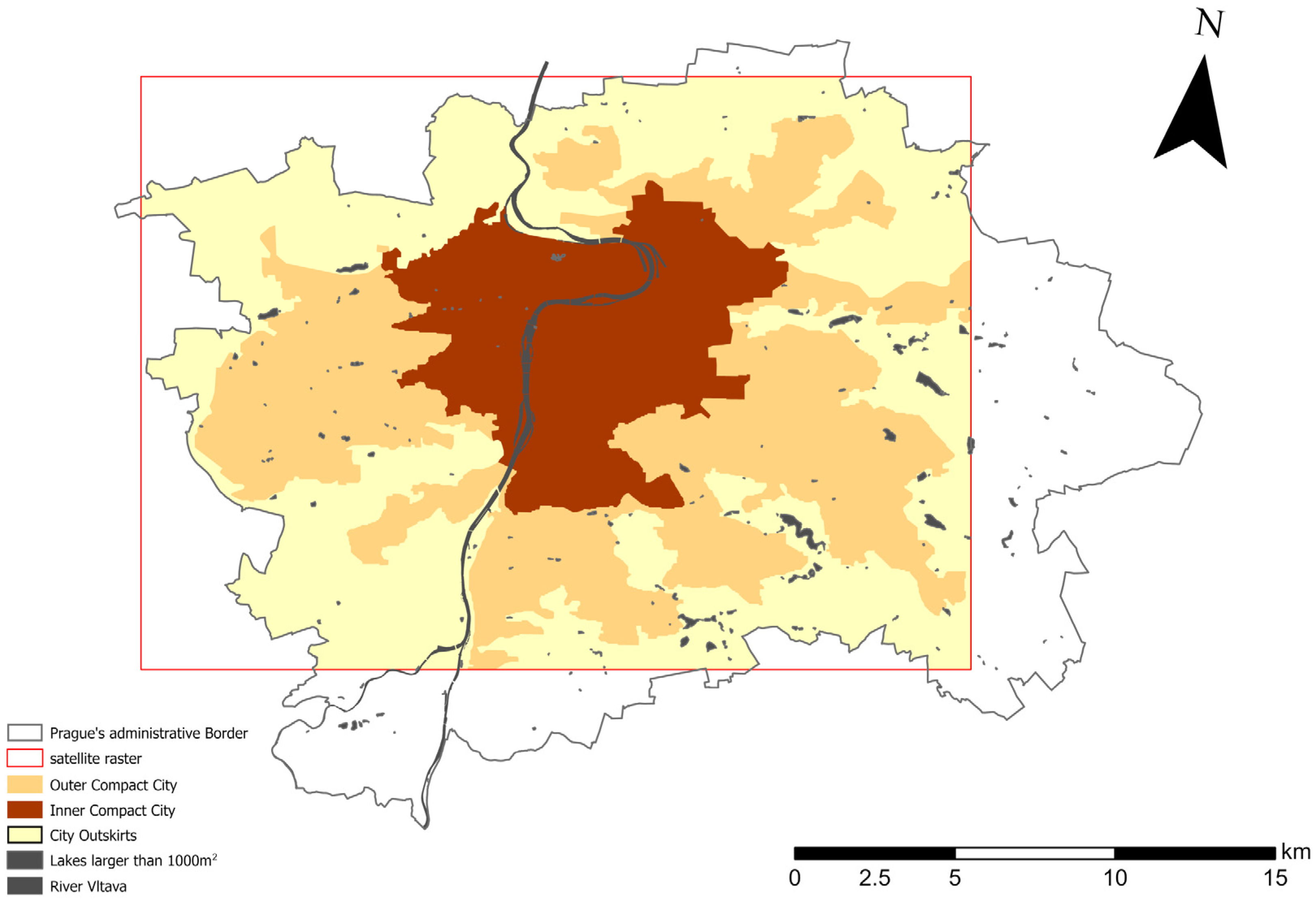
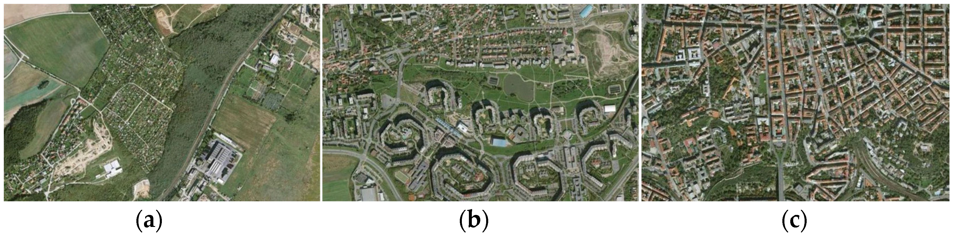
2.1. Study Area
2.2. Temperature Measurement
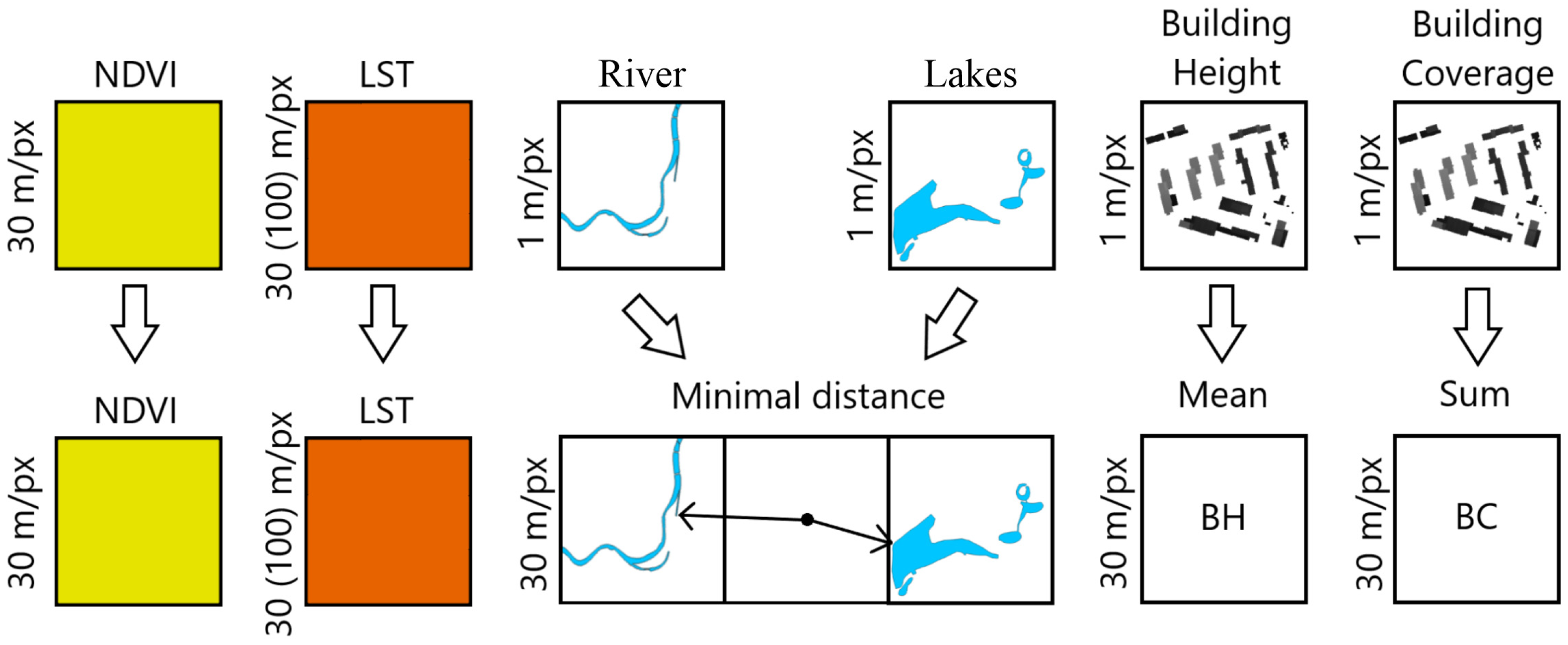
2.3. Creating Input Data (Factors) for Analysis
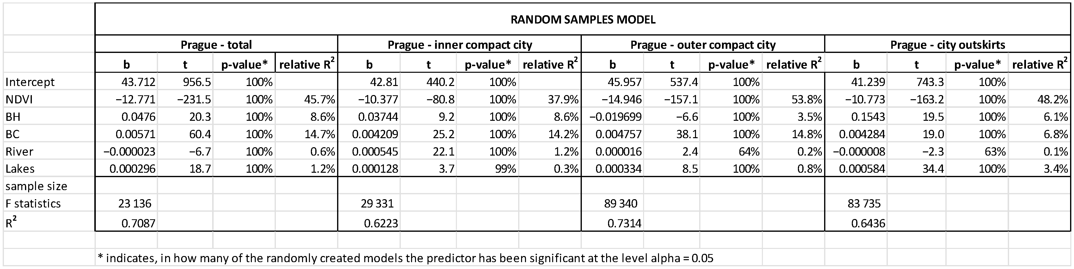
2.4. Statistical Analysis
3. Results
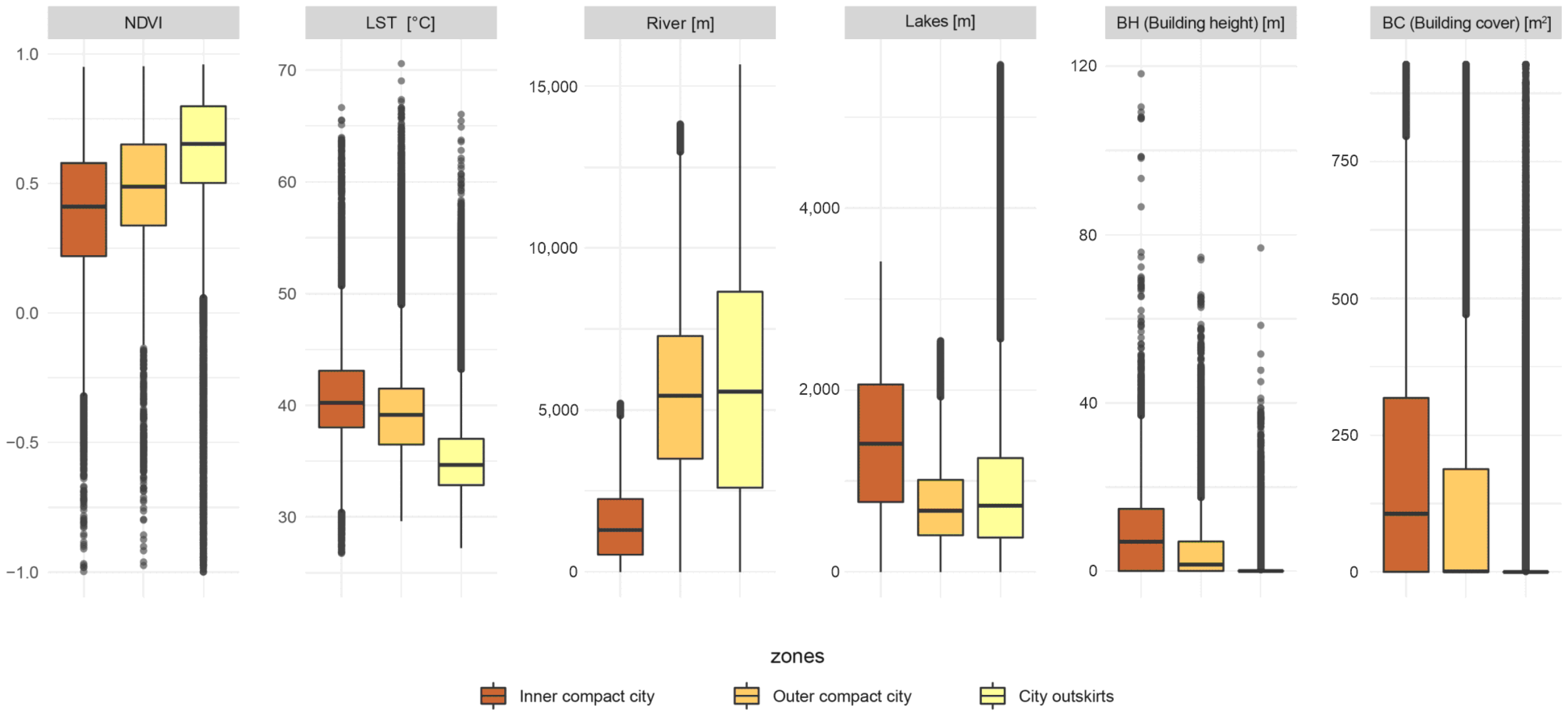
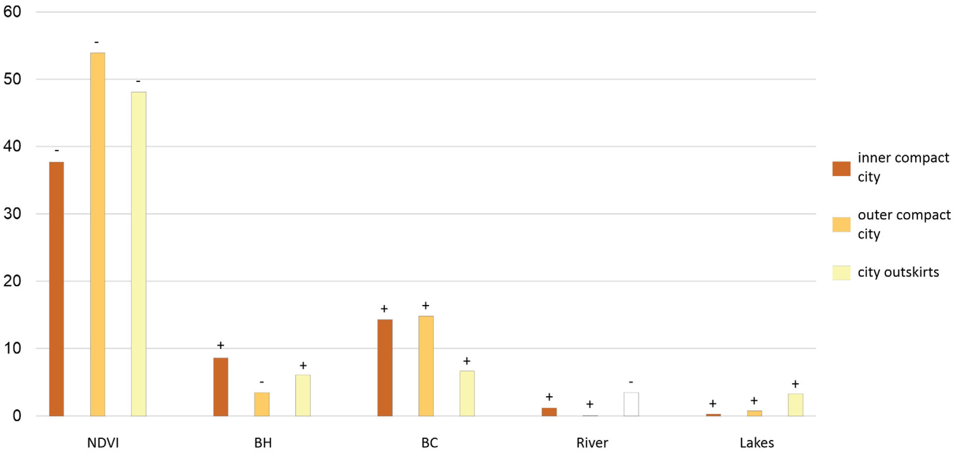
3.1. City Overview
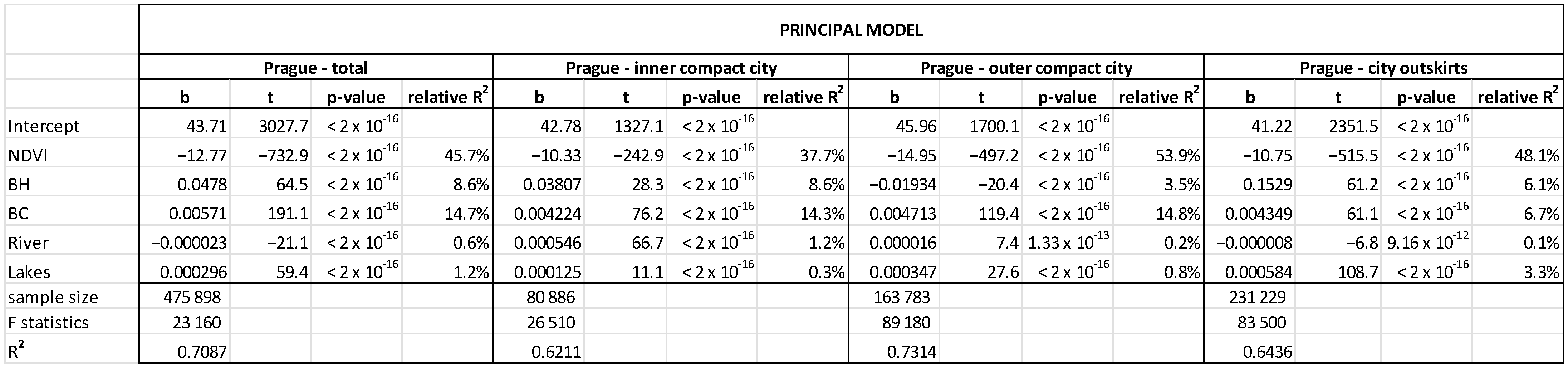
3.2. Association of LST and Individual Factors in Prague as a Whole (Principal Models)
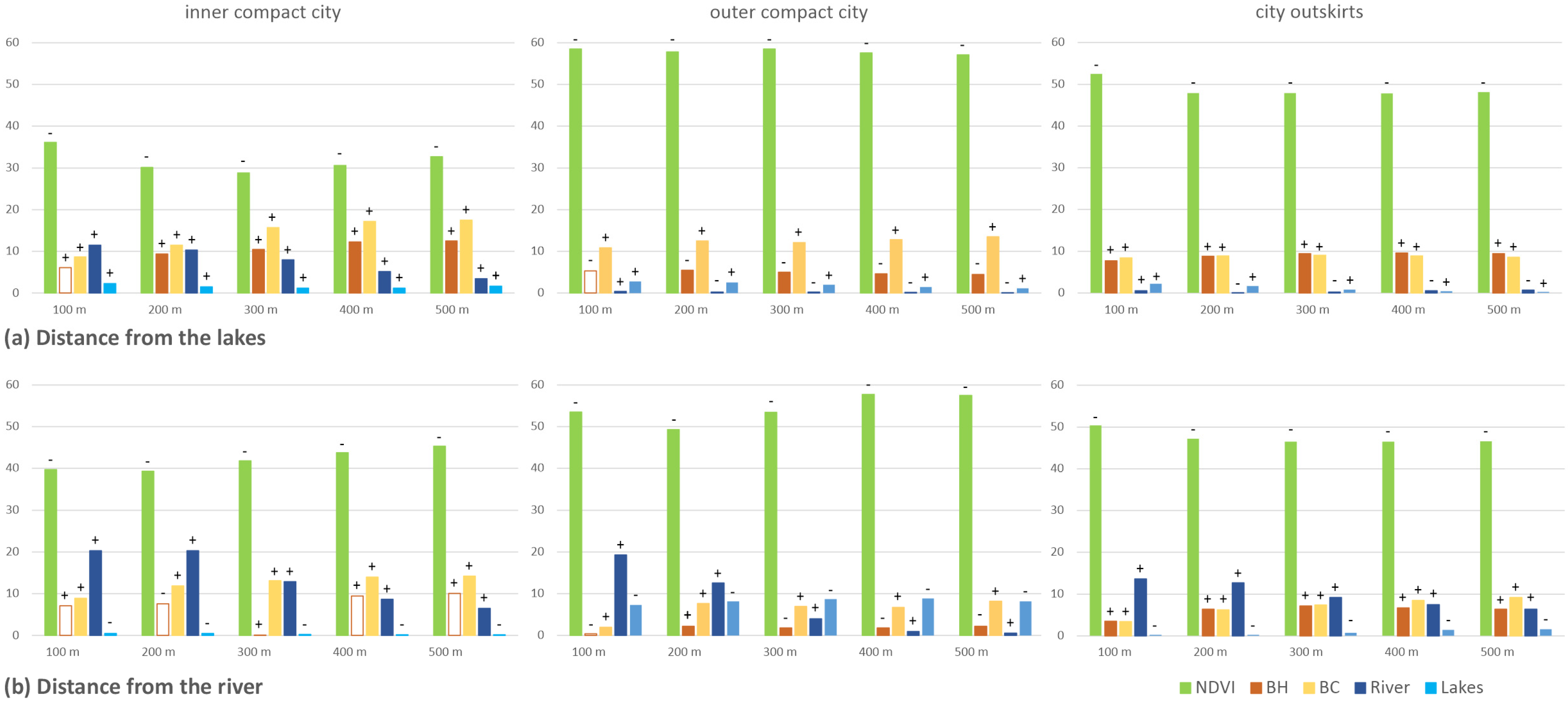
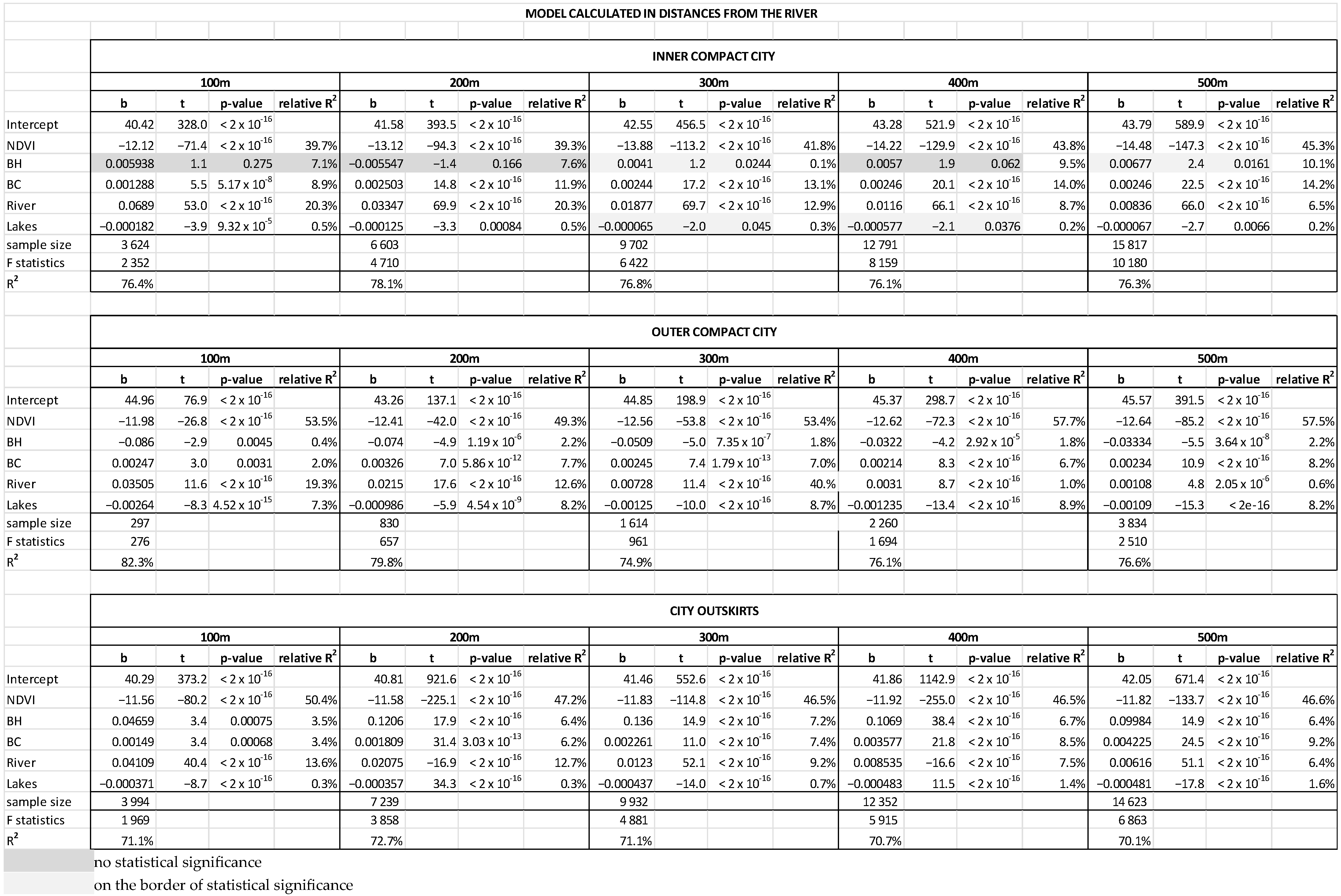
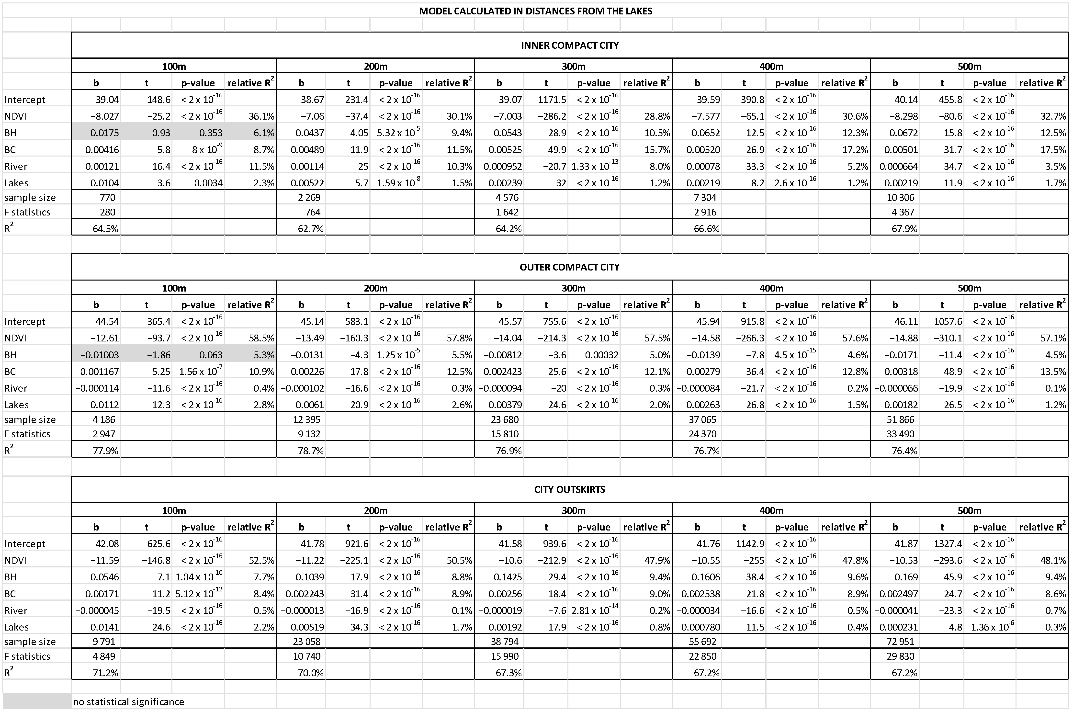
3.3. Association of LST and Individual Factors around the River and Lakes
4. Discussion
4.1. Comparing the Effect of the Green and Blue Bodies on LST
4.2. Comparing the Effect of the Lakes and the River on LST
4.3. Explaining Urban Morphology
4.4. Study Limitations and Further Research
5. Conclusions
Author Contributions
Funding
Data Availability Statement
Acknowledgments
Conflicts of Interest
Appendix A

Appendix B

Appendix C

Appendix D

References
- Sun, F.; Liu, M.; Wang, Y.; Wang, H.; Che, Y. The Effects of 3D Architectural Patterns on the Urban Surface Temperature at a Neighborhood Scale: Relative Contributions and Marginal Effects. J. Clean. Prod. 2020, 258, 120706. [Google Scholar] [CrossRef]
- Zhou, L.; Yuan, B.; Hu, F.; Wei, C.; Dang, X.; Sun, D. Understanding the Effects of 2D/3D Urban Morphology on Land Surface Temperature Based on Local Climate Zones. Build. Environ. 2022, 208, 108578. [Google Scholar] [CrossRef]
- Manoli, G.; Fatichi, S.; Schläpfer, M.; Yu, K.; Crowther, T.W.; Meili, N.; Burlando, P.; Katul, G.G.; Bou-Zeid, E. Magnitude of Urban Heat Islands Largely Explained by Climate and Population. Nature 2019, 573, 55–60. [Google Scholar] [CrossRef]
- Gunawardena, K.R.; Wells, M.J.; Kershaw, T. Utilising Green and Bluespace to Mitigate Urban Heat Island Intensity. Sci. Total Environ. 2017, 584–585, 1040–1055. [Google Scholar] [CrossRef]
- Bay, J.H.P.; Lehmann, S. Growing Compact: Urban Form, Density and Sustainability; Bay, J.H.P., Lehmann, S., Eds.; Routledge: Oxon, NY, USA, 2017. [Google Scholar]
- EC (European Commission). Green Paper: Towards a New Culture for Urban Mobility; Office for the Official Publications of the European Communities: Luxembourg, 2007. [Google Scholar]
- Assessment, A.C. Compact City Policies; OECD Publishing: Paris, France, 2012; ISBN 9789264167865. [Google Scholar]
- Urban, A.; Fonseca-Rodríguez, O.; Di Napoli, C.; Plavcová, E. Temporal Changes of Heat-Attributable Mortality in Prague, Czech Republic, over 1982–2019. Urban Clim. 2022, 44, 101197. [Google Scholar] [CrossRef]
- Ayanlade, A. Remote Sensing Approaches for Land Use and Land Surface Temperature Assessment: A Review of Methods. Int. J. Image Data Fusion 2017, 8, 188–210. [Google Scholar] [CrossRef]
- Gemitzi, A.; Dalampakis, P.; Falalakis, G. Detecting Geothermal Anomalies Using Landsat 8 Thermal Infrared Remotely Sensed Data. Int. J. Appl. Earth Obs. Geoinf. 2021, 96, 102283. [Google Scholar] [CrossRef]
- Wang, Y.; Zhan, Q.; Ouyang, W. Science of the Total Environment How to Quantify the Relationship between Spatial Distribution of Urban Waterbodies and Land Surface Temperature? Sci. Total Environ. 2019, 671, 1–9. [Google Scholar] [CrossRef] [PubMed]
- Guo, G.; Zhou, X.; Wu, Z.; Xiao, R.; Chen, Y. Characterizing the Impact of Urban Morphology Heterogeneity on Land Surface Temperature in Guangzhou, China. Environ. Model. Softw. 2016, 84, 427–439. [Google Scholar] [CrossRef]
- He, B.J.; Zhu, J.; Zhao, D.X.; Gou, Z.H.; da Qi, J.; Wang, J. Co-Benefits Approach: Opportunities for Implementing Sponge City and Urban Heat Island Mitigation. Land Use Policy 2019, 86, 147–157. [Google Scholar] [CrossRef]
- Badura, T.; Krkoška Lorencová, E.; Ferrini, S.; Vačkářová, D. Public Support for Urban Climate Adaptation Policy through Nature-Based Solutions in Prague. Landsc. Urban Plan. 2021, 215, 104215. [Google Scholar] [CrossRef]
- Ouyang, W.; Morakinyo, T.E.; Ren, C.; Ng, E. The Cooling Efficiency of Variable Greenery Coverage Ratios in Different Urban Densities: A Study in a Subtropical Climate. Build. Environ. 2020, 174, 106772. [Google Scholar] [CrossRef]
- Ghosh, S.; Das, A. Modelling Urban Cooling Island Impact of Green Space and Water Bodies on Surface Urban Heat Island in a Continuously Developing Urban Area. Model. Earth Syst. Environ. 2018, 4, 501–515. [Google Scholar] [CrossRef]
- Kirschner, V.; Macků, K.; Moravec, D.; Maňas, J. Measuring the Relationships between Various Urban Green Spaces and Local Climate Zones. Sci. Rep. 2023, 13, 9799. [Google Scholar] [CrossRef] [PubMed]
- Wang, Y.; Ouyang, W. Investigating the Heterogeneity of Water Cooling Effect for Cooler Cities. Sustain. Cities Soc. 2021, 75, 103281. [Google Scholar] [CrossRef]
- Jacobs, C.; Klok, L.; Bruse, M.; Cortesão, J.; Lenzholzer, S.; Kluck, J. Are Urban Water Bodies Really Cooling? Urban Clim. 2020, 32, 100607. [Google Scholar] [CrossRef]
- Lin, Y.; Wang, Z.; Jim, C.Y.; Li, J.; Deng, J.; Liu, J. Water as an Urban Heat Sink: Blue Infrastructure Alleviates Urban Heat Island Effect in Mega-City Agglomeration. J. Clean. Prod. 2020, 262, 121411. [Google Scholar] [CrossRef]
- Agathangelidis, I.; Cartalis, C.; Santamouris, M. Urban Morphological Controls on Surface Thermal Dynamics: A Comparative Assessment of Major European Cities with a Focus on Athens, Greece. Climate 2020, 8, 131. [Google Scholar] [CrossRef]
- Pang, B.; Zhao, J.; Zhang, J.; Yang, L. How to Plan Urban Green Space in Cold Regions of China to Achieve the Best Cooling Efficiency. Urban Ecosyst. 2022, 25, 1181–1198. [Google Scholar] [CrossRef]
- Grilo, F.; Pinho, P.; Aleixo, C.; Catita, C.; Silva, P.; Lopes, N.; Freitas, C.; Santos-Reis, M.; McPhearson, T.; Branquinho, C. Using Green to Cool the Grey: Modelling the Cooling Effect of Green Spaces with a High Spatial Resolution. Sci. Total Environ. 2020, 724, 138182. [Google Scholar] [CrossRef]
- Qiu, K.; Jia, B. The Roles of Landscape Both inside the Park and the Surroundings in Park Cooling Effect. Sustain. Cities Soc. 2020, 52, 101864. [Google Scholar] [CrossRef]
- Ferreira, L.S.; Duarte, D.H.S. Exploring the Relationship between Urban Form, Land Surface Temperature and Vegetation Indices in a Subtropical Megacity. Urban Clim. 2019, 27, 105–123. [Google Scholar] [CrossRef]
- Chen, W.; Zhang, J.; Shi, X.; Liu, S. Impacts of Building Features on the Cooling Effect of Vegetation in Community-Based Microclimate: Recognition, Measurement and Simulation from a Case Study of Beijing. Int. J. Environ. Res. Public. Health 2020, 17, 8915. [Google Scholar] [CrossRef] [PubMed]
- Straub, A.; Berger, K.; Breitner, S.; Cyrys, J.; Geruschkat, U.; Jacobeit, J.; Kühlbach, B.; Kusch, T.; Philipp, A.; Schneider, A.; et al. Statistical Modelling of Spatial Patterns of the Urban Heat Island Intensity in the Urban Environment of Augsburg, Germany. Urban Clim. 2019, 29, 100491. [Google Scholar] [CrossRef]
- Xue, Z.; Hou, G.; Zhang, Z.; Lyu, X.; Jiang, M.; Zou, Y.; Shen, X.; Wang, J.; Liu, X. Quantifying the Cooling-Effects of Urban and Peri-Urban Wetlands Using Remote Sensing Data: Case Study of Cities of Northeast China. Landsc. Urban Plan. 2019, 182, 92–100. [Google Scholar] [CrossRef]
- Zheng, Z.; Zhou, W.; Yan, J.; Qian, Y.; Wang, J.; Li, W. The Higher, the Cooler? Effects of Building Height on Land Surface Temperatures in Residential Areas of Beijing. Phys. Chem. Earth 2019, 110, 149–156. [Google Scholar] [CrossRef]
- Rahman, M.M.; Avtar, R.; Yunus, A.P.; Dou, J.; Misra, P.; Takeuchi, W.; Sahu, N.; Kumar, P.; Johnson, B.A.; Dasgupta, R.; et al. Monitoring Effect of Spatial Growth on Land Surface Temperature in Dhaka. Remote Sens. 2020, 12, 1191. [Google Scholar] [CrossRef]
- Yu, S.; Chen, Z.; Yu, B.; Wang, L.; Wu, B.; Wu, J.; Zhao, F. Exploring the Relationship between 2D/3D Landscape Pattern and Land Surface Temperature Based on Explainable EXtreme Gradient Boosting Tree: A Case Study of Shanghai, China. Sci. Total Environ. 2020, 725, 138229. [Google Scholar] [CrossRef]
- He, B.J.; Wang, J.; Zhu, J.; Qi, J. Beating the Urban Heat: Situation, Background, Impacts and the Way Forward in China. Renew. Sustain. Energy Rev. 2022, 161, 112350. [Google Scholar] [CrossRef]
- Alexander, C. Influence of the Proportion, Height and Proximity of Vegetation and Buildings on Urban Land Surface Temperature. Int. J. Appl. Earth Obs. Geoinf. 2021, 95, 102265. [Google Scholar] [CrossRef]
- COM. Green Paper on the Urban Environment; Commission of the European Communities: Luxembourg, 1990. [Google Scholar]
- Štěpánek, P.; Trnka, M.; Meitner, J.; Dubrovský, M.; Zahradníček, P.; Lhotka, O.; Skalák, P.; Kyselý, J.; Farda, A.; Semerádová, D. Očekávané Klimatické Podmínky v České Republice Část I. Změna Základních Parametrů; Czech Globe: Brno, Czech Republic, 2019. [Google Scholar]
- ČHMÚ. Výroční Zpráva ČHMÚ; ČHMÚ: Prague, Czech Republic, 2019. [Google Scholar]
- Ouředníček, M.; Pospíšilová, L.; Špačková, P.; Temelová, J.; Novák, J. Prostorová Typologie a Zonace Prahy. In Sociální Proměny Pražských Čtvrtí (Social Change of the Cities); Ouředníček, M., Temelová, J., Eds.; Academia: Prague, Czech Republic, 2012; pp. 268–286. [Google Scholar]
- Yang, Q.; Huang, X.; Tang, Q. The Footprint of Urban Heat Island Effect in 302 Chinese Cities: Temporal Trends and Associated Factors. Sci. Total Environ. 2019, 655, 652–662. [Google Scholar] [CrossRef]
- van de Griend, A.A.; Owe, M. On the Relationship between Thermal Emissivity and the Normalized Difference Vegetation Index for Natural Surfaces. Int. J. Remote Sens. 1993, 14, 1119–1131. [Google Scholar] [CrossRef]
- Asgarian, A.; Amiri, B.J.; Sakieh, Y. Assessing the Effect of Green Cover Spatial Patterns on Urban Land Surface Temperature Using Landscape Metrics Approach. Urban Ecosyst. 2015, 18, 209–222. [Google Scholar] [CrossRef]
- Cooley, T.; Anderson, G.P.; Felde, G.W.; Hoke, M.L.; Ratkowski, A.J.; Chetwynd, J.H.; Gardner, J.A.; Adler-Golden, S.M.; Matthew, M.W.; Berk, A.; et al. FLAASH, a MODTRAN4-Based Atmospheric Correction Algorithm, Its Application and Validation. In Proceedings of the IEEE International Geoscience and Remote Sensing Symposium, Toronto, ON, Canada, 24–28 June 2002; Volume 3, pp. 1414–1418. [Google Scholar]
- Azen, R.; Budescu, D.V. The Dominance Analysis Approach for Comparing Predictors in Multiple Regression. Psychol. Methods 2003, 8, 129–148. [Google Scholar] [CrossRef]
- Karimi Firozjaei, M.; Kiavarz, M.; Alavipanah, S.K. Impact of Surface Characteristics and Their Adjacency Effects on Urban Land Surface Temperature in Different Seasonal Conditions and Latitudes. Build. Environ. 2022, 219, 109145. [Google Scholar] [CrossRef]
- Kovář, P. Ekosystémová a Krajinná Ekologie; Charles University, Karolinum: Prague, Czech Republic, 2014; ISBN 978-80-246-2788-5. [Google Scholar]
- Zhang, Z.; Paschalis, A.; Mijic, A.; Meili, N.; Manoli, G.; van Reeuwijk, M.; Fatichi, S. A Mechanistic Assessment of Urban Heat Island Intensities and Drivers across Climates. Urban Clim. 2022, 44, 101215. [Google Scholar] [CrossRef]
- Fedor, T.; Hofierka, J. Comparison of Urban Heat Island Diurnal Cycles under Various Atmospheric Conditions Using WRF-UCM. Atmosphere 2022, 13, 2057. [Google Scholar] [CrossRef]
- Chen, J.; Zhan, W.; Du, P.; Li, L.; Li, J.; Liu, Z.; Huang, F. Seasonally Disparate Responses of Surface Thermal Environment to 2D / 3D Urban Morphology. Build. Environ. 2022, 214, 108928. [Google Scholar] [CrossRef]
- Anselin, L. Spatial Econometrics. In A Companion to Theoretical Econometrics; Baltagi, B.H., Ed.; Blackwell Publishing Ltd.: Hoboken, NJ, USA, 2003. [Google Scholar]
- Anselin, L. Spatial Econometrics: Methods and Models, 1st ed.; Springer: Dordrecht, The Netherlands, 1988. [Google Scholar]
- Brunsdon, C.; Fotheringham, S.; Charlton, M. Geographically Weighted Regression. J. R. Stat. Soc. Ser. D (Stat.) 1998, 47, 431–443. [Google Scholar] [CrossRef]
- Brunsdon, C.; Fotheringham, A.S.; Charlton, M.E. Geographically Weighted Regression: A Method for Exploring Spatial Nonstationarity. Geogr. Anal. 1996, 28, 281–298. [Google Scholar] [CrossRef]
- Stewart, I.D.; Oke, T.R. Local Climate Zones for Urban Temperature Studies. Bull. Am. Meteorol. Soc. 2012, 93, 1879–1900. [Google Scholar] [CrossRef]


Disclaimer/Publisher’s Note: The statements, opinions and data contained in all publications are solely those of the individual author(s) and contributor(s) and not of MDPI and/or the editor(s). MDPI and/or the editor(s) disclaim responsibility for any injury to people or property resulting from any ideas, methods, instructions or products referred to in the content. |
© 2024 by the authors. Licensee MDPI, Basel, Switzerland. This article is an open access article distributed under the terms and conditions of the Creative Commons Attribution (CC BY) license (https://creativecommons.org/licenses/by/4.0/).
Share and Cite
Kirschner, V.; Moravec, D.; Macků, K.; Kozhoridze, G.; Komárek, J. Comparing the Effects of Green and Blue Bodies and Urban Morphology on Land Surface Temperatures Close to Rivers and Large Lakes. Land 2024, 13, 162. https://doi.org/10.3390/land13020162
Kirschner V, Moravec D, Macků K, Kozhoridze G, Komárek J. Comparing the Effects of Green and Blue Bodies and Urban Morphology on Land Surface Temperatures Close to Rivers and Large Lakes. Land. 2024; 13(2):162. https://doi.org/10.3390/land13020162
Chicago/Turabian StyleKirschner, Vlad’ka, David Moravec, Karel Macků, Giorgi Kozhoridze, and Jan Komárek. 2024. "Comparing the Effects of Green and Blue Bodies and Urban Morphology on Land Surface Temperatures Close to Rivers and Large Lakes" Land 13, no. 2: 162. https://doi.org/10.3390/land13020162