

Dynamic Impact of Urban Built Environment on Land Surface Temperature Considering Spatio-Temporal Heterogeneity: A Perspective of Local Climate Zone


Abstract
:1. Introduction
2. Materials and Methods
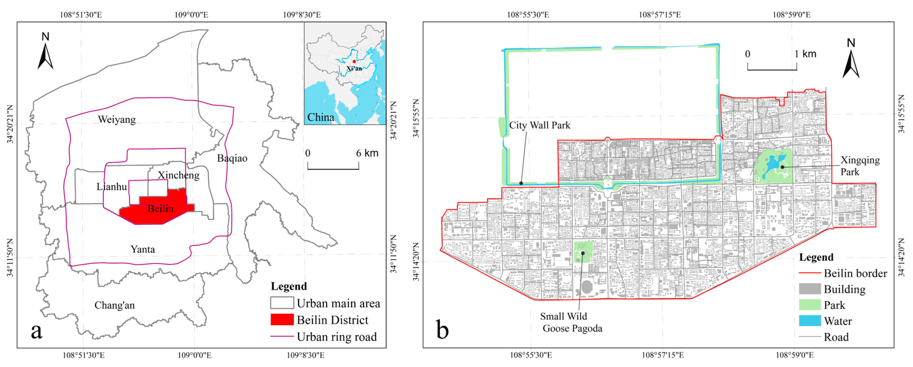
2.1. Study Area
2.2. Data Source and Processing
2.2.1. Land Surface Temperature
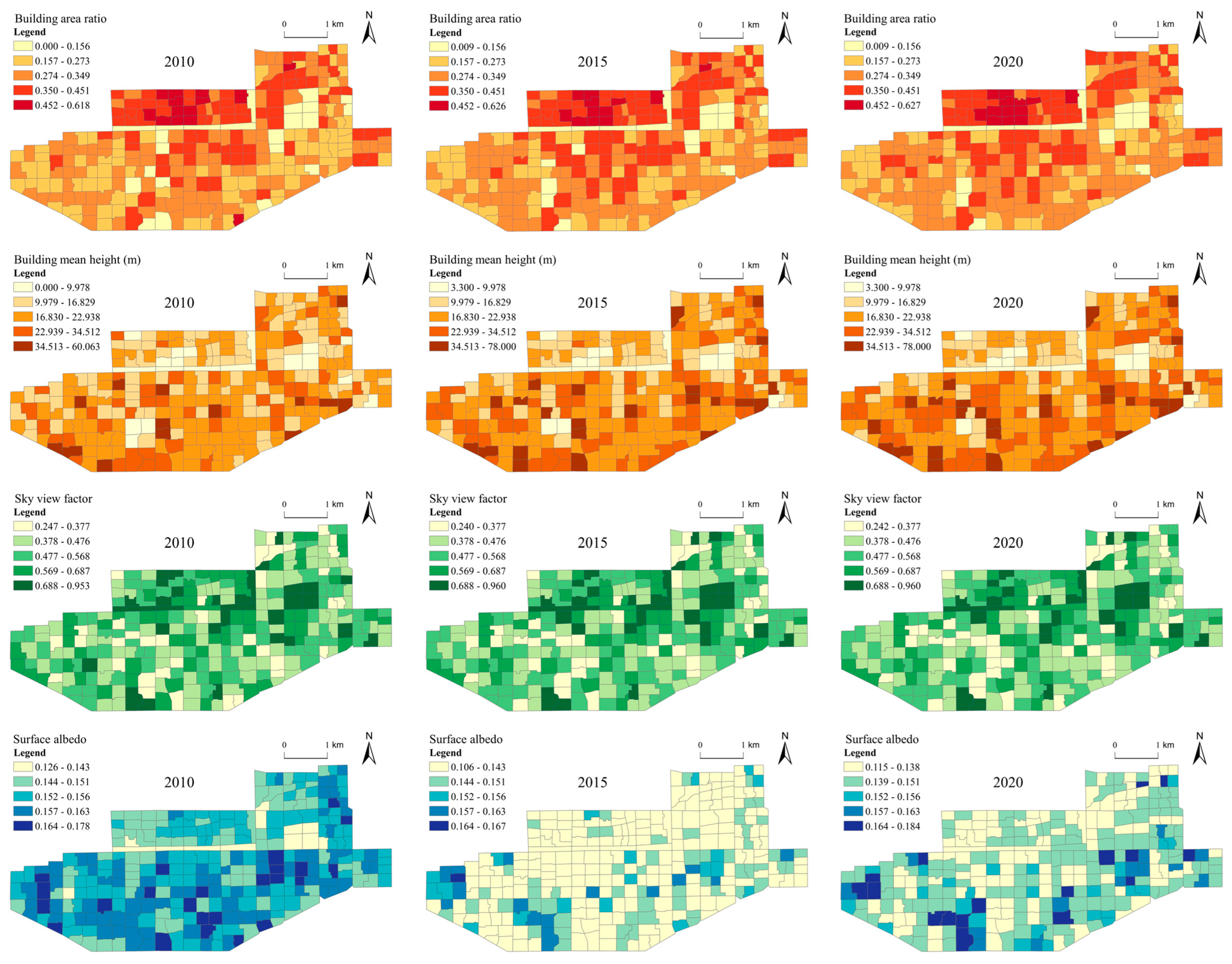
2.2.2. Built Environment Dataset
2.3. Methods
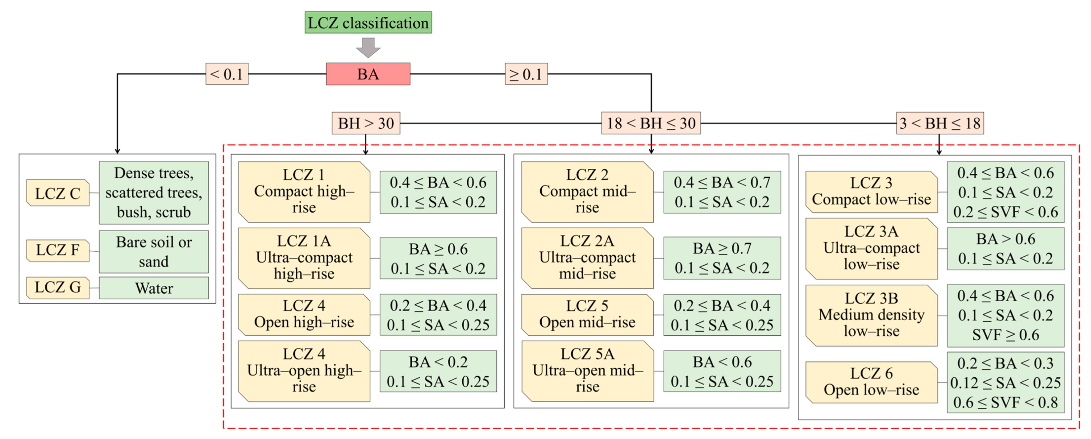
2.3.1. Local Climate Zone Classification
2.3.2. Driving Indicators

| Type | Indicator | Calculation Formula | Physical Meaning | Reference |
|---|---|---|---|---|
| Urban 2D morphology | Vegetation cover ratio (VC) | Reflects the vegetation cover. | [95] | |
| Impervious surface area ratio (ISA) | Reflects the coverage of impervious surface. | [96] | ||
| Urban 3D morphology | Building mean height (BH) | Reflects the overall height of buildings. | [17,29,35,36,97] | |
| Building area ratio (BA) | Reflects the density of buildings. | [17,29,35,36,97] | ||
| Building mean volume (BV) | Reflects the space occupied by buildings. | [29,35,85] | ||
| Space congestion degree (SC) | Reflects the congestion degree of buildings. | [35] | ||
| Floor area ratio (FAR) | Reflects the construction intensity of buildings. | [35] | ||
| Sky view factor (SVF) | Reflects the sky openness. | [36,97,98] |
2.3.3. Geodetector
2.3.4. Geographically Weighted Regression
3. Results
3.1. LCZ Types
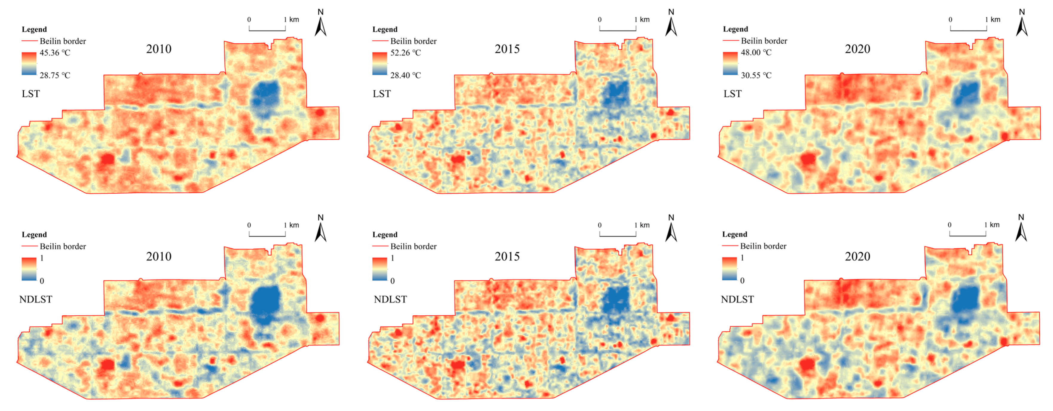
3.2. Spatio-Temporal Evolution Characteristics of LST
3.2.1. Temporal Variation of LST
3.2.2. Spatial Changing Characteristics of LST
3.3. Influence Effect Based on Geodetector
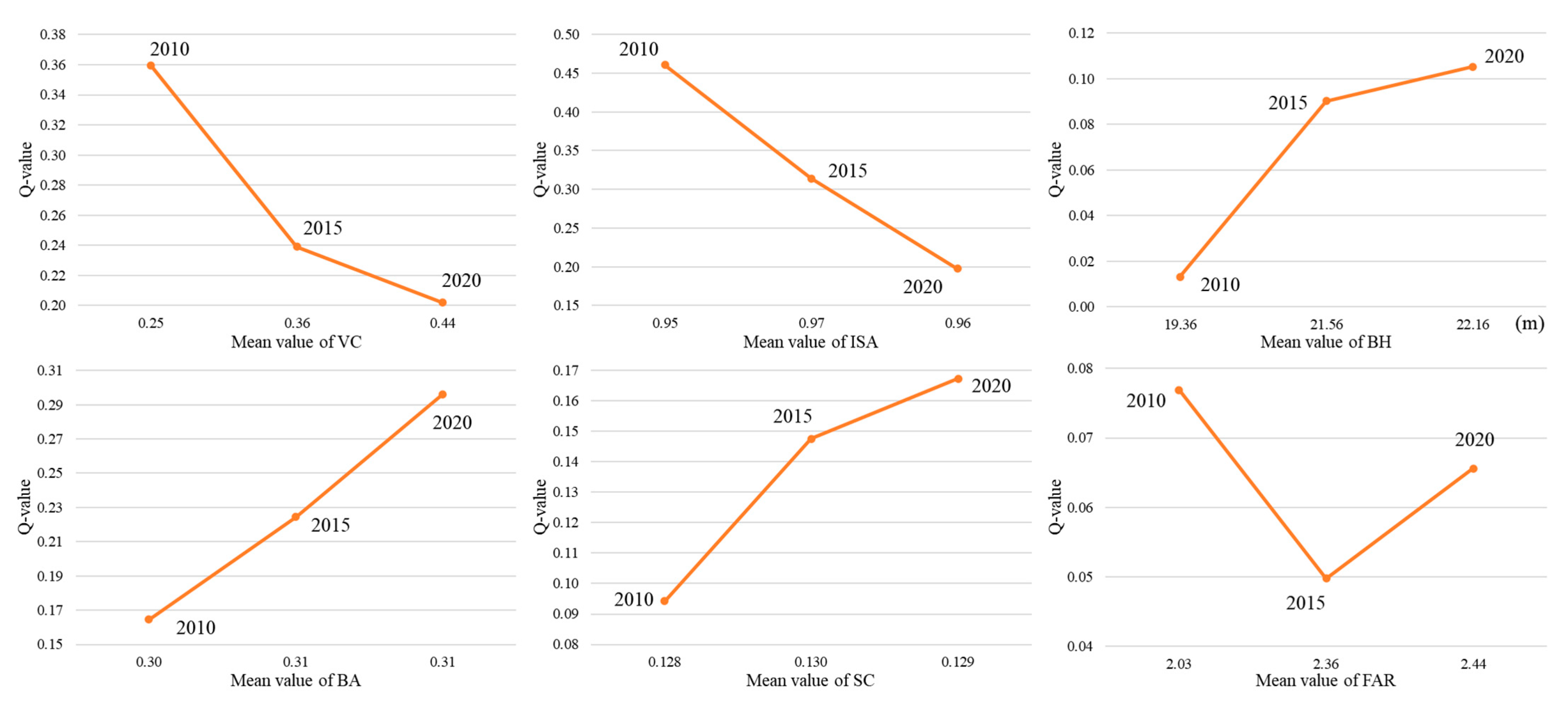
3.3.1. Factor Detection
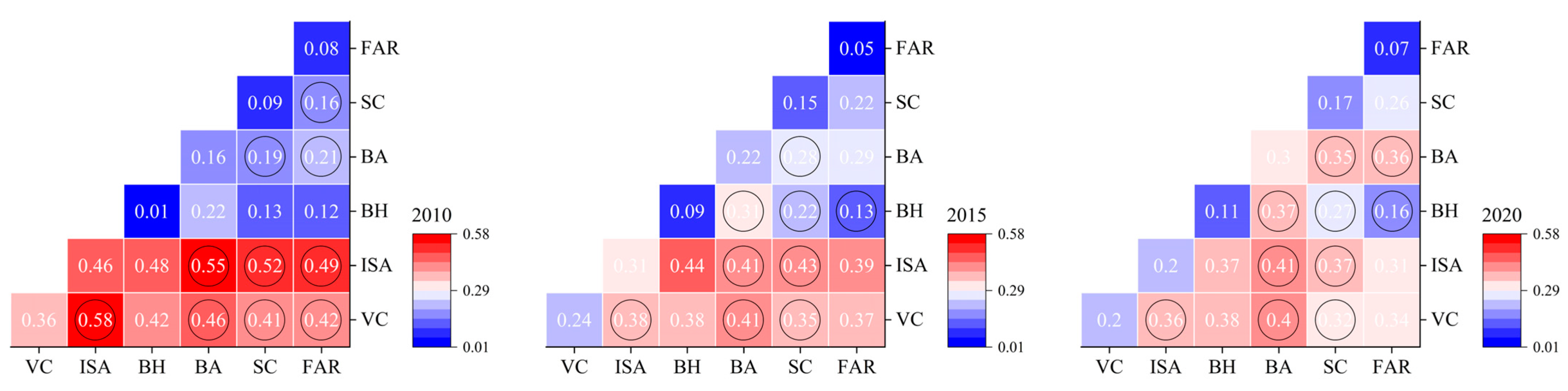
3.3.2. Interaction Detection
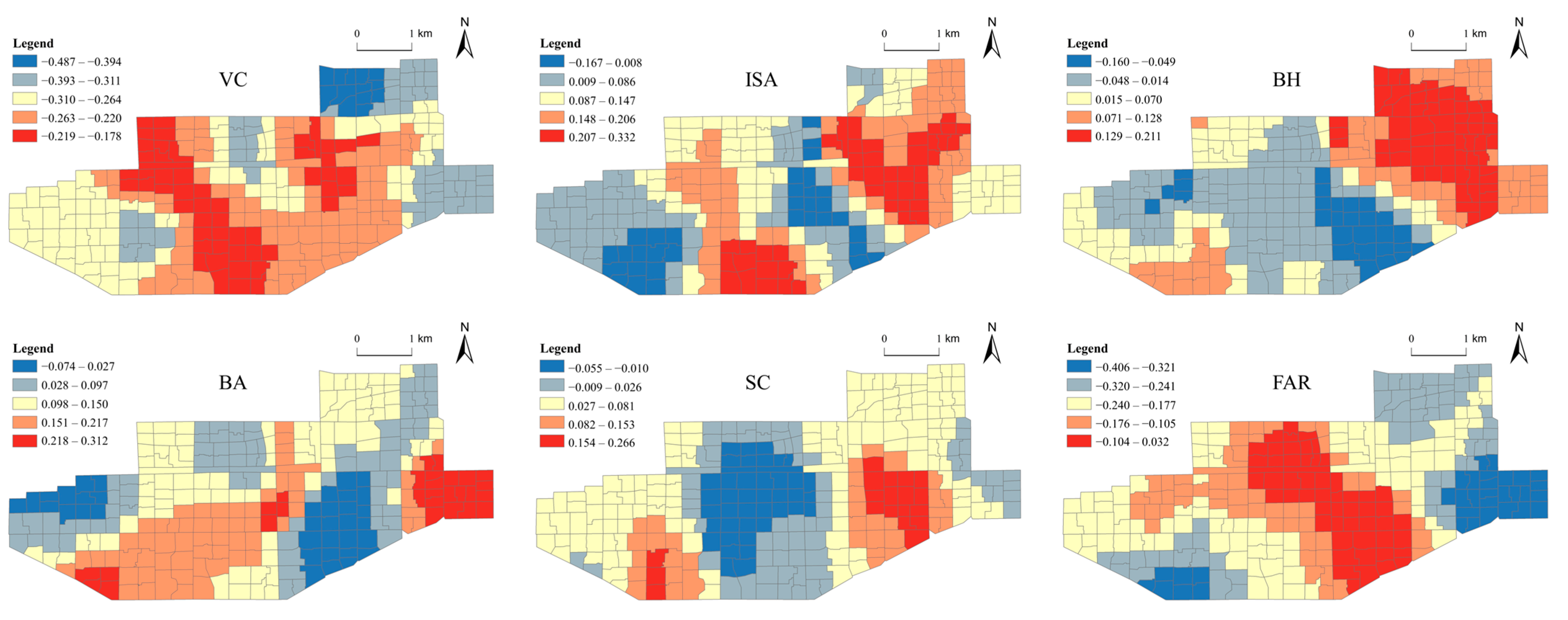
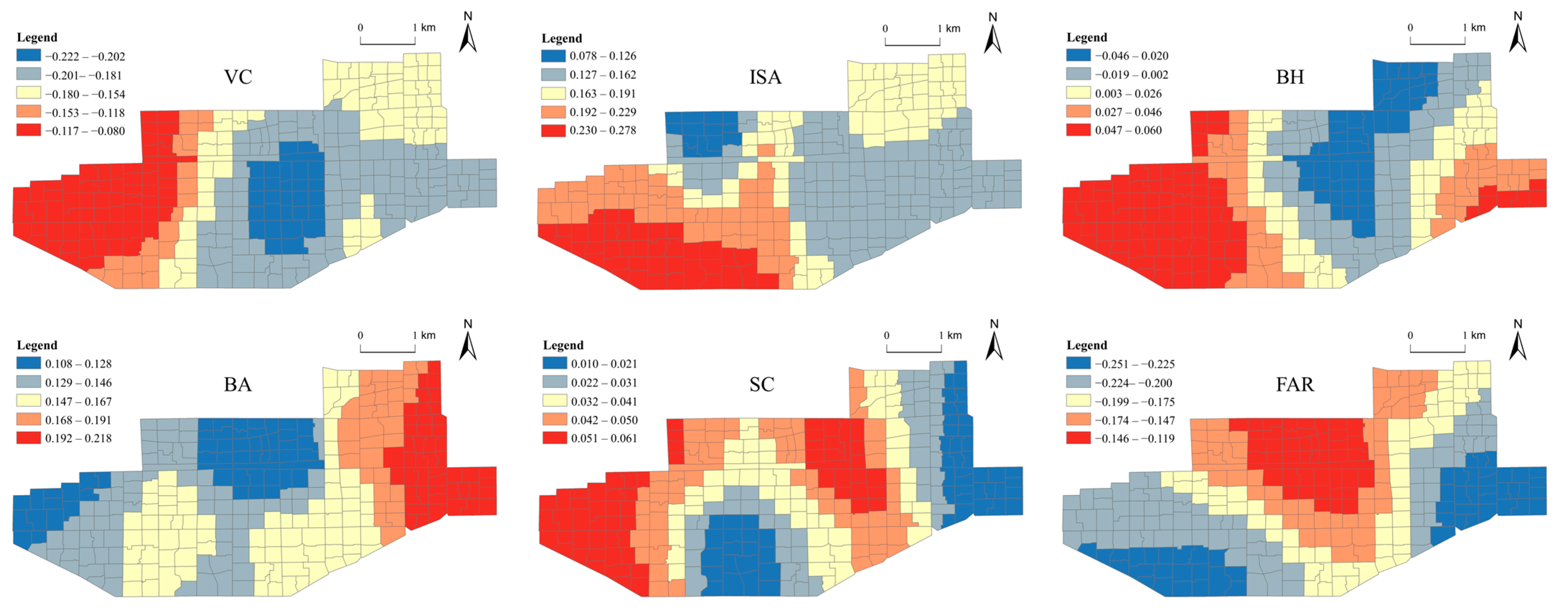
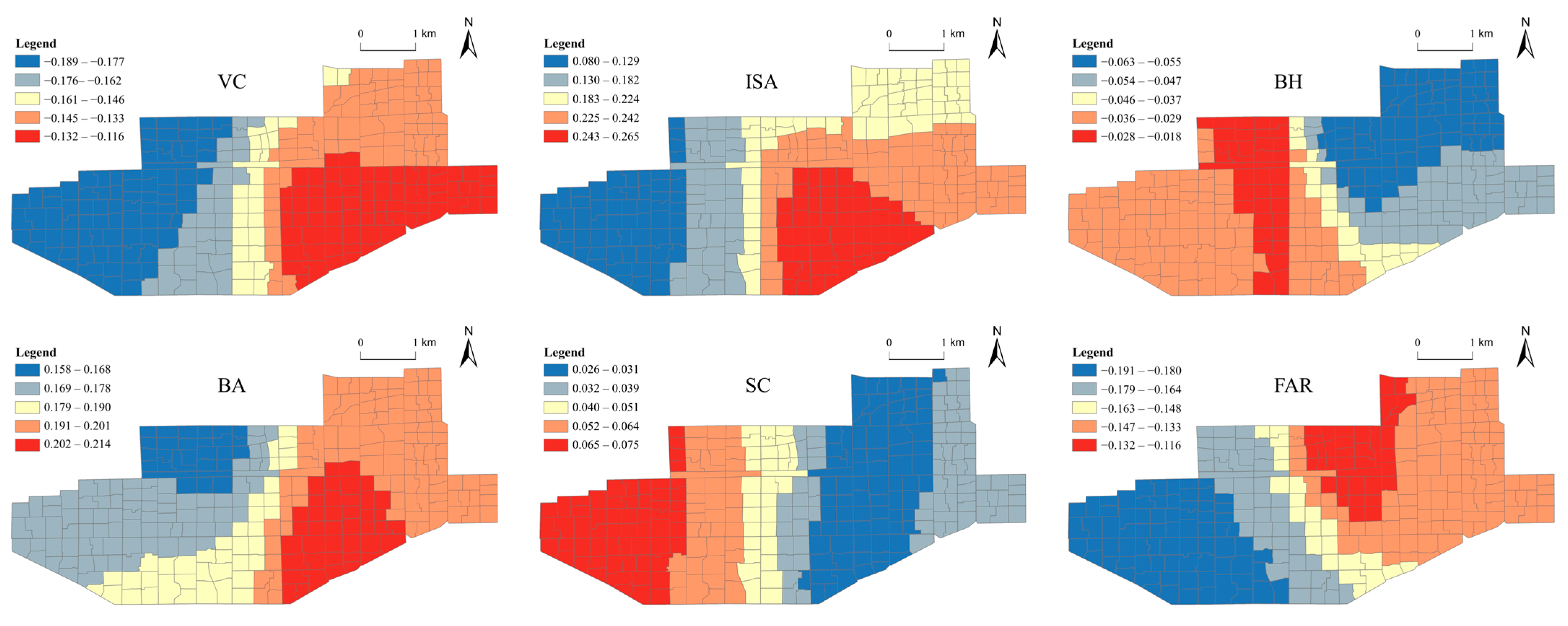
3.4. Influence Effect Based on GWR
4. Discussion
4.1. Spatial Differentiation of LST in Different LCZs
4.2. Impact Effect of Built Environment on LST
4.3. Optimal Solution of Impact Effect on LST
4.4. Insights and Shortcomings
5. Conclusions
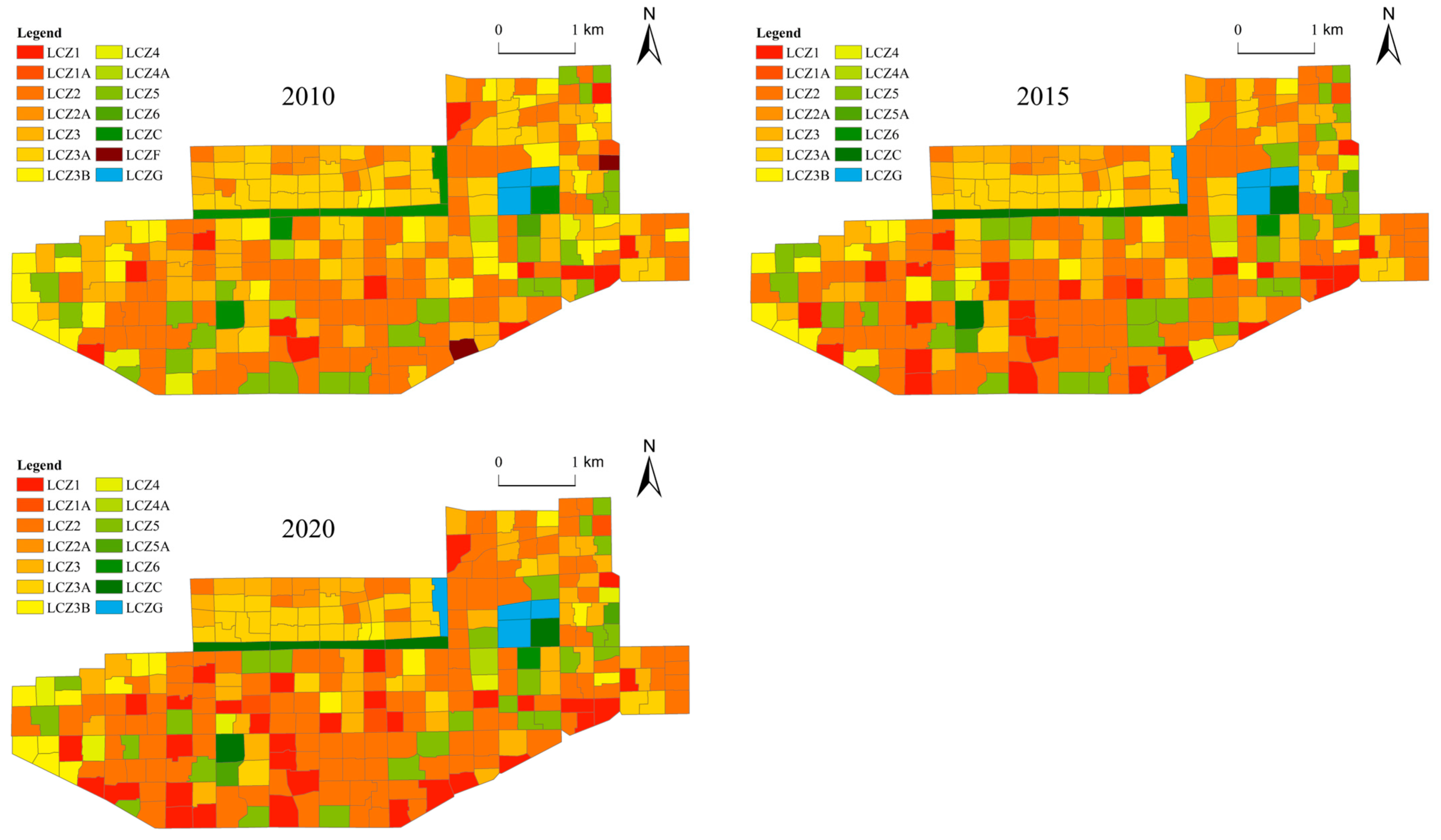
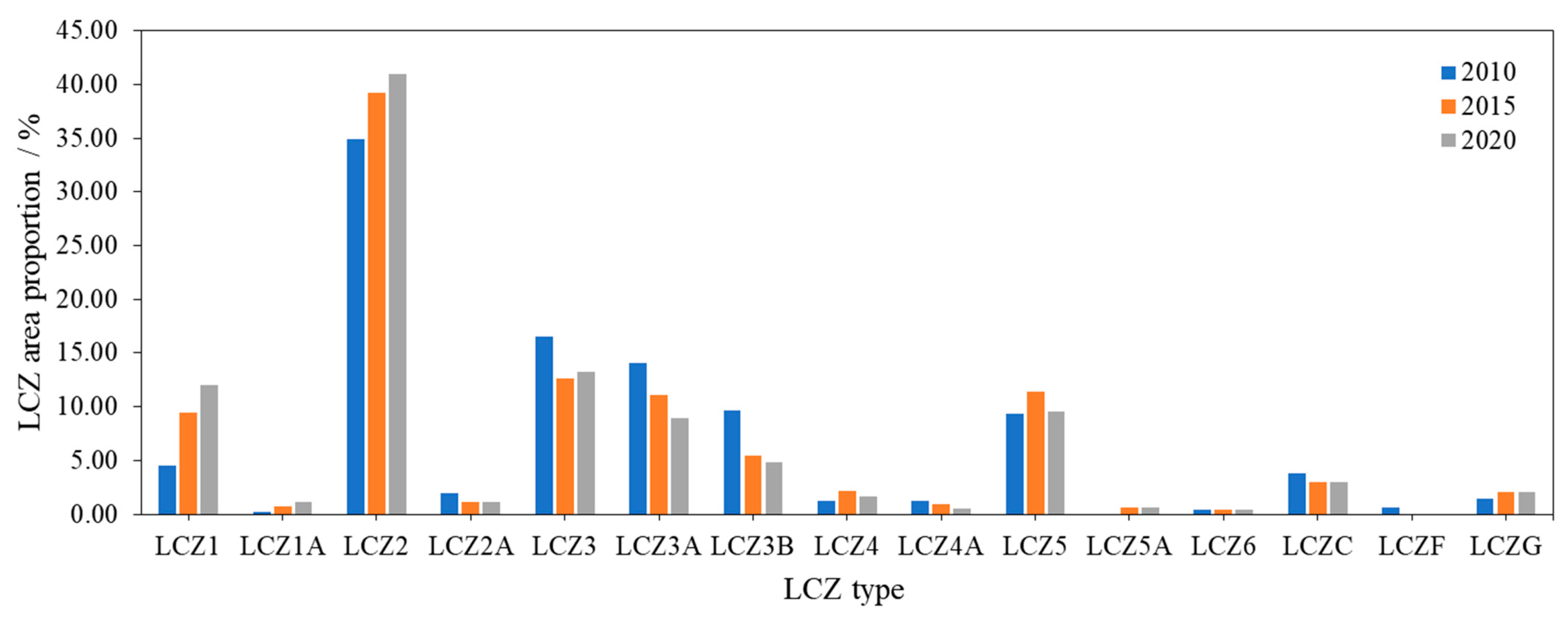
- (1)
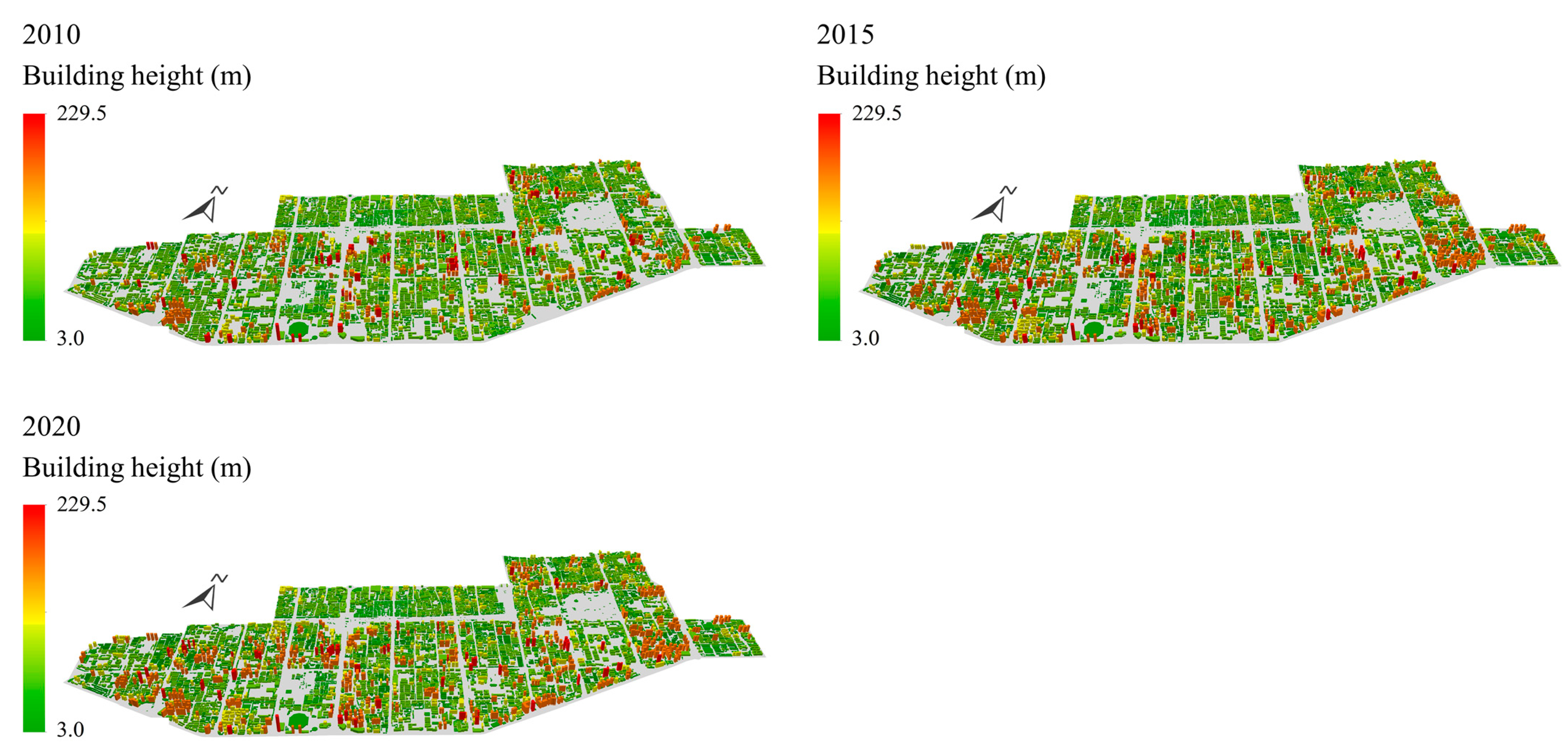
- In Beilin District, 15, 14, and 14 LCZ types were found in the years 2010, 2015, and 2020, respectively. Dense building zones in Beilin District account for a large share in the area, while open building zones and natural surface zones account for a small share. From 2010 to 2020, the area of mid- and high-rise dense building zones continues to increase, while the area of low-rise dense building zones continues to decrease.
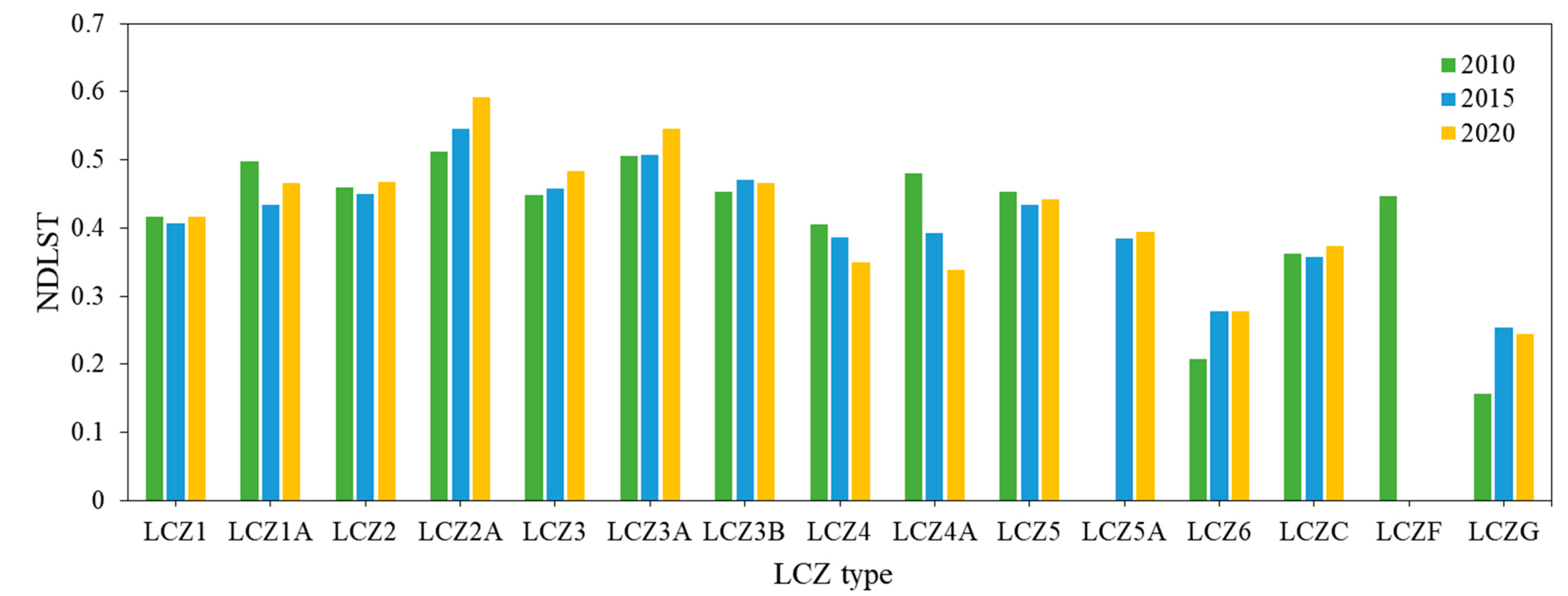
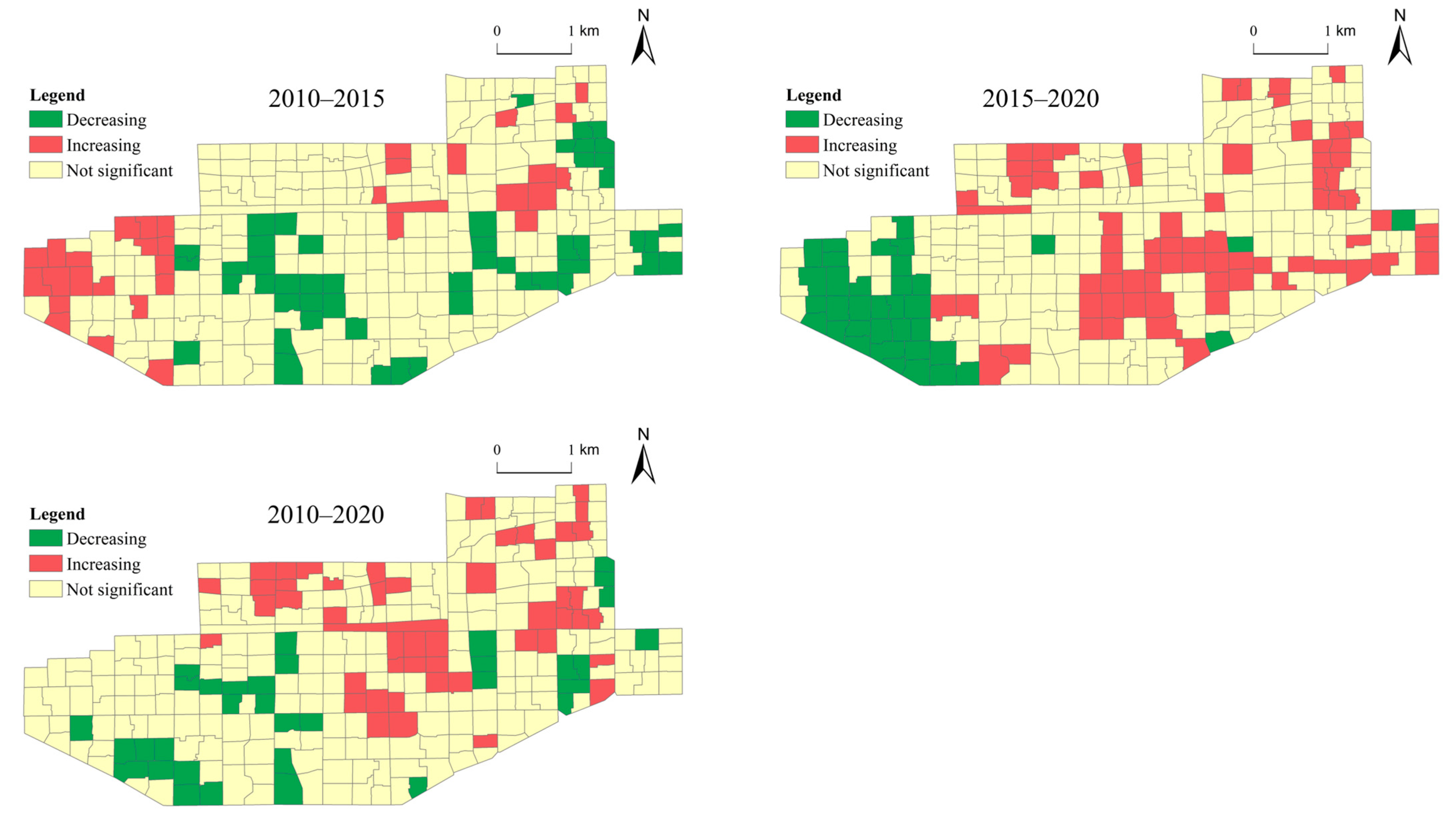
- (2)
- The LST of different LCZ types in Beilin District is markedly different. The LST of dense building zones is generally higher than that of open building zones and natural surface zones. The LST of mid- and low-rise dense building zones increased gradually, while the LST of high-rise open building zones decreased gradually. The warming area of Beilin District is obviously more than the cooling area.
- (3)
- The 2D built environment indicators had a larger force on the LST than 3D indicators. The force of VC decreased from 0.36 to 0.20 and ISA from 0.46 to 0.20; the force of BA increased from 0.16 to 0.30 and SC from 0.09 to 0.17; the force of FAR was relatively stable at 0.07–0.08; and the force of BH changed from insignificant to significant. The interaction of the built environment on the LST showed an enhancement effect, which was greater for 2D than for 3D indicators. The force of VC and ISA gradually decreased, while the force of BH, BA, and SC gradually increased, and FAR was relatively stable.
- (4)
- VC and FAR showed negative effects, with the average action intensity of VC decreasing from −0.27 to −0.15, FAR from −0.20 to −0.16. ISA, BA, and SC showed positive effects, with the average action intensity of ISA increasing from 0.12 to 0.20 and BA from 0.12 to 0.19. SC remained stable at 0.04. BH gradually acted from positively to negatively, with the average action intensity changing from 0.05 to −0.04.
Author Contributions
Funding
Data Availability Statement
Conflicts of Interest
Appendix A

Appendix B
| Visual | LCZ 1 | LCZ 1A | LCZ 2 | LCZ 3 | LCZ 3A | LCZ 3B | LCZ 4 | LCZ 4A | LCZ 5 | LCZ C | LCZ G | Total Zone | Mapping Accuracy (%) | |
|---|---|---|---|---|---|---|---|---|---|---|---|---|---|---|
| GIS | ||||||||||||||
| LCZ 1 | 1 | 0 | 0 | 0 | 0 | 0 | 0 | 0 | 0 | 0 | 0 | 1 | 100 | |
| LCZ 1A | 1 | 0 | 0 | 0 | 0 | 0 | 0 | 0 | 0 | 0 | 0 | 1 | 0 | |
| LCZ 2 | 0 | 0 | 13 | 2 | 0 | 0 | 0 | 0 | 0 | 0 | 0 | 15 | 86.7 | |
| LCZ 3 | 0 | 0 | 1 | 7 | 1 | 0 | 0 | 0 | 1 | 0 | 0 | 10 | 70 | |
| LCZ 3A | 0 | 0 | 0 | 0 | 6 | 0 | 0 | 0 | 0 | 0 | 0 | 6 | 100 | |
| LCZ 3B | 0 | 0 | 0 | 0 | 0 | 5 | 0 | 0 | 0 | 0 | 0 | 5 | 100 | |
| LCZ 4 | 0 | 0 | 0 | 0 | 0 | 0 | 0 | 1 | 0 | 0 | 0 | 1 | 0 | |
| LCZ 4A | 0 | 0 | 0 | 0 | 0 | 0 | 0 | 0 | 1 | 0 | 0 | 1 | 0 | |
| LCZ 5 | 0 | 0 | 0 | 1 | 0 | 1 | 0 | 0 | 6 | 0 | 0 | 8 | 75 | |
| LCZ C | 0 | 0 | 0 | 0 | 0 | 0 | 0 | 0 | 0 | 1 | 0 | 1 | 100 | |
| LCZ G | 0 | 0 | 0 | 0 | 0 | 0 | 0 | 0 | 0 | 0 | 1 | 1 | 100 | |
| Total Zone | 2 | 0 | 14 | 10 | 7 | 6 | 0 | 1 | 8 | 1 | 1 | 50 | ||
| Mapping accuracy (%) | 50 | 0 | 93 | 70 | 86 | 83 | 0 | 0 | 75 | 100 | 100 | |||
| Visual | LCZ 1 | LCZ 1A | LCZ 2 | LCZ 2A | LCZ 3 | LCZ 3A | LCZ 3B | LCZ 4A | LCZ 5 | LCZ C | LCZ G | Total Zone | Mapping Accuracy (%) | |
|---|---|---|---|---|---|---|---|---|---|---|---|---|---|---|
| GIS | ||||||||||||||
| LCZ 1 | 7 | 0 | 0 | 0 | 0 | 0 | 0 | 0 | 0 | 0 | 0 | 7 | 100 | |
| LCZ 1A | 1 | 0 | 0 | 0 | 0 | 0 | 0 | 0 | 0 | 0 | 0 | 1 | 0 | |
| LCZ 2 | 0 | 0 | 16 | 0 | 0 | 0 | 0 | 0 | 0 | 0 | 0 | 16 | 100 | |
| LCZ 2A | 0 | 0 | 0 | 1 | 0 | 0 | 0 | 0 | 0 | 0 | 0 | 1 | 100 | |
| LCZ 3 | 0 | 0 | 0 | 0 | 4 | 0 | 0 | 0 | 0 | 0 | 0 | 4 | 100 | |
| LCZ 3A | 0 | 0 | 0 | 0 | 0 | 8 | 0 | 0 | 0 | 0 | 0 | 8 | 100 | |
| LCZ 3B | 0 | 0 | 0 | 0 | 1 | 0 | 2 | 0 | 0 | 0 | 0 | 3 | 67 | |
| LCZ 4A | 0 | 0 | 0 | 0 | 0 | 1 | 0 | 1 | 0 | 0 | 0 | 2 | 50 | |
| LCZ 5 | 0 | 0 | 0 | 0 | 0 | 0 | 1 | 0 | 5 | 0 | 0 | 6 | 83 | |
| LCZ C | 0 | 0 | 0 | 0 | 0 | 0 | 0 | 0 | 0 | 1 | 0 | 1 | 100 | |
| LCZ G | 0 | 0 | 0 | 0 | 0 | 0 | 0 | 0 | 0 | 0 | 1 | 1 | 100 | |
| Total Zone | 8 | 0 | 16 | 1 | 5 | 9 | 3 | 1 | 5 | 1 | 1 | 50 | ||
| Mapping accuracy (%) | 88 | 0 | 100 | 100 | 80 | 89 | 67 | 100 | 100 | 100 | 100 | |||
| Visual | LCZ 1 | LCZ 1A | LCZ 2 | LCZ 2A | LCZ 3 | LCZ 3A | LCA 3B | LCZ 4 | LCZ 4A | LCZ 5 | Total Zone | Mapping Accuracy (%) | |
|---|---|---|---|---|---|---|---|---|---|---|---|---|---|
| GIS | |||||||||||||
| LCZ 1 | 2 | 0 | 0 | 0 | 0 | 0 | 0 | 0 | 0 | 0 | 2 | 1 | |
| LCZ 1A | 1 | 1 | 1 | 0 | 0 | 0 | 0 | 0 | 0 | 0 | 3 | 33 | |
| LCZ 2 | 0 | 0 | 21 | 0 | 0 | 0 | 0 | 0 | 0 | 0 | 21 | 1 | |
| LCZ 2A | 0 | 0 | 1 | 0 | 0 | 1 | 0 | 0 | 0 | 0 | 2 | 0 | |
| LCZ 3 | 0 | 0 | 1 | 0 | 7 | 0 | 0 | 0 | 0 | 0 | 8 | 88 | |
| LCZ 3A | 0 | 0 | 0 | 0 | 0 | 4 | 1 | 0 | 0 | 0 | 5 | 80 | |
| LCA 3B | 0 | 0 | 0 | 0 | 0 | 0 | 2 | 0 | 0 | 0 | 2 | 100 | |
| LCZ 4 | 0 | 0 | 0 | 0 | 0 | 0 | 0 | 1 | 0 | 0 | 1 | 100 | |
| LCZ 4A | 1 | 0 | 0 | 0 | 0 | 0 | 0 | 0 | 3 | 0 | 4 | 75 | |
| LCZ 5 | 0 | 0 | 0 | 0 | 0 | 0 | 0 | 0 | 0 | 2 | 2 | 100 | |
| Total Zone | 4 | 1 | 24 | 0 | 7 | 5 | 3 | 1 | 3 | 2 | 50 | ||
| Mapping accuracy (%) | 50 | 1 | 88 | 0 | 1 | 80 | 66 | 100 | 100 | 100 | |||
Appendix C


References
- IPCC. Climate Change 2022: Mitigation of Climate Change. Contribution of Working Group III to the Sixth Assessment Report of the Intergovernmental Panel on Climate Change; Cambridge University Press: Cambridge, UK; New York, NY, USA , 2022. [Google Scholar]
- Rizwan, A.M.; Dennis, L.Y.C.; Liu, C. A review on the generation, determination and mitigation of urban heat island. J. Environ. Sci. 2008, 20, 120–128. [Google Scholar] [CrossRef] [PubMed]
- Li, X.; Zhou, Y.; Yu, S.; Jia, G.; Li, H.; Li, W. Urban heat island impacts on building energy consumption: A review of approaches and findings. Energy 2019, 174, 407–419. [Google Scholar] [CrossRef]
- Agarwal, M.; Tandon, A. Modeling of the urban heat island in the form of mesoscale wind and of its effect on air pollution dispersal. Appl. Math. Model. 2010, 34, 2520–2530. [Google Scholar] [CrossRef]
- Wong, K.V.; Paddon, A.; Jimenez, A. Review of world urban heat islands: Many linked to increased mortality. J. Energy Resour. Technol. 2013, 135, 022101. [Google Scholar] [CrossRef]
- Shahfahad; Naikoo, M.W.; Towfiqul Islam, A.R.M.; Mallick, J.; Rahman, A. Land use/land cover change and its impact on surface urban heat island and urban thermal comfort in a metropolitan city. Urban Clim. 2022, 41, 101052. [Google Scholar] [CrossRef]
- Krehbiel, C.P.; Jackson, T.; Henebry, G.M. Web-enabled landsat data time series for monitoring urban heat island impacts on land surface phenology. IEEE J. Sel. Top. Appl. Earth Obs. Remote Sens. 2016, 9, 2043–2050. [Google Scholar] [CrossRef]
- Weng, Q. Remote sensing of impervious surfaces in the urban areas: Requirements, methods, and trends. Remote Sens. Environ. 2012, 117, 34–49. [Google Scholar] [CrossRef]
- Mohan, M.; Kandya, A. Impact of urbanization and land-use/land-cover change on diurnal temperature range: A case study of tropical urban airshed of India using remote sensing data. Sci. Total Environ. 2015, 506–507, 453–465. [Google Scholar] [CrossRef]
- Dai, Z.; Guldmann, J.M.; Hu, Y. Spatial regression models of park and land-use impacts on the urban heat island in central Beijing. Sci. Total Environ. 2018, 626, 1136–1147. [Google Scholar] [CrossRef]
- Kamali Maskooni, E.; Hashemi, H.; Berndtsson, R.; Daneshkar Arasteh, P.; Kazemi, M. Impact of spatiotemporal land-use and land-cover changes on surface urban heat islands in a semiarid region using Landsat data. Int. J. Digit. Earth 2021, 14, 250–270. [Google Scholar] [CrossRef]
- Mansour, K.; Aziz, M.A.; Hashim, S.; Effat, H. Impact of anthropogenic activities on urban heat islands in major cities of El-Minya Governorate, Egypt. Egypt. J. Remote Sens. Space Sci. 2022, 25, 609–620. [Google Scholar] [CrossRef]
- Marković, M.; Cheema, J.; Teofilović, A.; Čepić, S.; Popović, Z.; Tomićević-Dubljević, J.; Pause, M. Monitoring of spatiotemporal change of green spaces in relation to the land surface temperature: A case study of Belgrade, Serbia. Remote Sens. 2021, 13, 3846. [Google Scholar] [CrossRef]
- Zhu, Z.; Shen, Y.; Fu, W.; Zheng, D.; Huang, P.; Li, J.; Lan, Y.; Chen, Z.; Liu, Q.; Xu, X.; et al. How does 2D and 3D of urban morphology affect the seasonal land surface temperature in Island City? A block-scale perspective. Ecol. Indic. 2023, 150, 110221. [Google Scholar] [CrossRef]
- Huang, X.; Wang, Y. Investigating the effects of 3D urban morphology on the surface urban heat island effect in urban functional zones by using high-resolution remote sensing data: A case study of Wuhan, central China. ISPRS J. Photogramm. Remote Sens. 2019, 152, 119–131. [Google Scholar] [CrossRef]
- Zhou, R.; Xu, H.; Zhang, H.; Zhang, J.; Liu, M.; He, T.; Gao, J.; Li, C. Quantifying the relationship between 2D/3D building patterns and land surface temperature: Study on the metropolitan Shanghai. Remote Sens. 2022, 14, 4098. [Google Scholar] [CrossRef]
- Li, X.; Yang, B.; Xu, G.; Liang, F.; Jiang, T.; Dong, Z. Exploring the impact of 2-D/3-D building morphology on the land surface temperature: A case study of three megacities in China. IEEE J. Sel. Top. Appl. Earth Obs. Remote Sens. 2021, 14, 4933–4945. [Google Scholar] [CrossRef]
- Kolokotsa, D.; Lilli, K.; Gobakis, K.; Mavrigiannaki, A.; Haddad, S.; Garshasbi, S.; Mohajer, H.R.H.; Paolini, R.; Vasilakopoulou, K.; Bartesaghi, C.; et al. Analyzing the impact of urban planning and building typologies in urban heat island mitigation. Buildings 2022, 12, 537. [Google Scholar] [CrossRef]
- Elkhazindar, A.; Kharrufa, S.N.; Arar, M.S. The effect of urban form on the heat island phenomenon and human thermal comfort: A comparative study of UAE residential sites. Energies 2022, 15, 5471. [Google Scholar] [CrossRef]
- Wu, Z.; Tong, Z.; Wang, M.; Long, Q. Assessing the impact of urban morphological parameters on land surface temperature in the heat aggregation areas with spatial heterogeneity: A case study of Nanjing. Build. Environ. 2023, 235, 110232. [Google Scholar] [CrossRef]
- Gao, Y.; Zhao, J.; Han, L. Exploring the spatial heterogeneity of urban heat island effect and its relationship to block morphology with the geographically weighted regression model. Sustain. Cities Soc. 2022, 76, 103431. [Google Scholar] [CrossRef]
- Hidalgo-García, D.; Arco-Díaz, J. Modeling the surface urban heat island (SUHI) to study of its relationship with variations in the thermal field and with the indices of land use in the metropolitan area of Granada (Spain). Sustain. Cities Soc. 2022, 87, 104166. [Google Scholar] [CrossRef]
- Ghosh, S.; Kumar, D.; Kumari, R. Assessing spatiotemporal variations in land surface temperature and SUHI intensity with a cloud based computational system over five major cities of India. Sustain. Cities Soc. 2022, 85, 104060. [Google Scholar] [CrossRef]
- Deng, X.; Gao, F.; Liao, S.; Liu, Y.; Chen, W. Spatiotemporal evolution patterns of urban heat island and its relationship with urbanization in Guangdong-Hong Kong-Macao greater bay area of China from 2000 to 2020. Ecol. Indic. 2023, 146, 109817. [Google Scholar] [CrossRef]
- Abd-Elmabod, S.K.; Jiménez-González, M.A.; Jordán, A.; Zhang, Z.; Mohamed, E.S.; Hammam, A.A.; El Baroudy, A.A.; Abdel-Fattah, M.K.; Abdelfattah, M.A.; Jones, L. Past and future impacts of urbanisation on land surface temperature in Greater Cairo over a 45 year period. Egypt. J. Remote Sens. Space Sci. 2022, 25, 961–974. [Google Scholar] [CrossRef]
- Liu, X.; Ming, Y.; Liu, Y.; Yue, W.; Han, G. Influences of landform and urban form factors on urban heat island: Comparative case study between Chengdu and Chongqing. Sci. Total Environ. 2022, 820, 153395. [Google Scholar] [CrossRef]
- Gu, Y.; You, X.-y. A spatial quantile regression model for driving mechanism of urban heat island by considering the spatial dependence and heterogeneity: An example of Beijing, China. Sustain. Cities Soc. 2022, 79, 103692. [Google Scholar] [CrossRef]
- Yu, X.; Xu, G.; Liu, Y.; Xiao, R. Influences of 3D features of buildings on land surface temperature: A case study in the Yangtze River Delta urban agglomeration. China Environ. Sci. 2021, 41, 5806–5816. [Google Scholar] [CrossRef]
- Cao, S.; Cai, Y.; Du, M.; Weng, Q.; Lu, L. Seasonal and diurnal surface urban heat islands in China: An investigation of driving factors with three-dimensional urban morphological parameters. GISci. Remote Sens. 2022, 59, 1121–1142. [Google Scholar] [CrossRef]
- Wang, J.; Meng, F.; Lu, H.; Lv, Y.; Jing, T. Individual and combined effects of 3D buildings and green spaces on the urban thermal environment: A case study in Jinan, China. Atmosphere 2023, 14, 908. [Google Scholar] [CrossRef]
- Liu, Y.; Xu, Y.; Zhang, F.; Shu, W. Influence of Beijing spatial morphology on the distribution of urban heat island. Acta Geogr. Sin. 2021, 76, 1662–1679. [Google Scholar] [CrossRef]
- Yan, G.; Su, J.; Guan, D. The impact of urban architectural vertical characteristics on urban thermal environment in Zhongshan District, Dalian. Sci. Geogr. Sin. 2019, 39, 125–130. [Google Scholar] [CrossRef]
- Hou, H.; Su, H.; Yao, C.; Wang, Z. Spatiotemporal patterns of the impact of surface roughness and morphology on urban heat island. Sustain. Cities Soc. 2023, 92, 104513. [Google Scholar] [CrossRef]
- Zheng, Y.; Ren, C.; Shi, Y.; Yim, S.H.L.; Lai, D.Y.F.; Xu, Y.; Fang, C.; Li, W. Mapping the spatial distribution of nocturnal urban heat island based on local climate zone framework. Build. Environ. 2023, 234, 110197. [Google Scholar] [CrossRef]
- Yu, X.; Liu, Y.; Zhang, Z.; Xiao, R. Influences of buildings on urban heat island based on 3D landscape metrics: An investigation of China’s 30 megacities at micro grid-cell scale and macro city scale. Landsc. Ecol. 2021, 36, 2743–2762. [Google Scholar] [CrossRef]
- Yang, L.; Yu, K.; Ai, J.; Liu, Y.; Yang, W.; Liu, J. Dominant factors and spatial heterogeneity of land surface temperatures in urban areas: A case study in Fuzhou, China. Remote Sens. 2022, 14, 1266. [Google Scholar] [CrossRef]
- Kim, J.; Lee, D.K.; Brown, R.D.; Kim, S.; Kim, J.H.; Sung, S. The effect of extremely low sky view factor on land surface temperatures in urban residential areas. Sustain. Cities Soc. 2022, 80, 103799. [Google Scholar] [CrossRef]
- Lu, H.; Li, F.; Yang, G.; Sun, W. Multi-scale impacts of 2D/3D urban building pattern in intra-annual thermal environment of Hangzhou, China. Int. J. Appl. Earth Obs. Geoinf. 2021, 104, 102558. [Google Scholar] [CrossRef]
- Chen, Y.; Yang, J.; Yu, W.; Ren, J.; Xiao, X.; Xia, J.C. Relationship between urban spatial form and seasonal land surface temperature under different grid scales. Sustain. Cities Soc. 2023, 89, 104374. [Google Scholar] [CrossRef]
- Yang, C.; Zhu, W.; Sun, J.; Xu, X.; Wang, R.; Lu, Y.; Zhang, S.; Zhou, W. Assessing the effects of 2D/3D urban morphology on the 3D urban thermal environment by using multi-source remote sensing data and UAV measurements: A case study of the snow-climate city of Changchun, China. J. Clean. Prod. 2021, 321, 128956. [Google Scholar] [CrossRef]
- Zhang, N.; Zhang, J.; Chen, W.; Su, J. Block-based variations in the impact of characteristics of urban functional zones on the urban heat island effect: A case study of Beijing. Sustain. Cities Soc. 2022, 76, 103529. [Google Scholar] [CrossRef]
- Wang, Q.; Wang, X.; Meng, Y.; Zhou, Y.; Wang, H. Exploring the impact of urban features on the spatial variation of land surface temperature within the diurnal cycle. Sustain. Cities Soc. 2023, 91, 104432. [Google Scholar] [CrossRef]
- Hu, Y.; Dai, Z.; Guldmann, J.M. Modeling the impact of 2D/3D urban indicators on the urban heat island over different seasons: A boosted regression tree approach. J. Environ. Manag. 2020, 266, 110424. [Google Scholar] [CrossRef] [PubMed]
- Han, S.; Hou, H.; Estoque, R.C.; Zheng, Y.; Shen, C.; Murayama, Y.; Pan, J.; Wang, B.; Hu, T. Seasonal effects of urban morphology on land surface temperature in a three-dimensional perspective: A case study in Hangzhou, China. Build. Environ. 2023, 228, 109913. [Google Scholar] [CrossRef]
- Stewart, I.D.; Oke, T.R. Local climate zones for urban temperature studies. Bull. Am. Meteorol. Soc. 2012, 93, 1879–1900. [Google Scholar] [CrossRef]
- Wang, R.; Cai, M.; Ren, C.; Bechtel, B.; Xu, Y.; Ng, E. Detecting multi-temporal land cover change and land surface temperature in Pearl River Delta by adopting local climate zone. Urban Clim. 2019, 28, 100455. [Google Scholar] [CrossRef]
- Zheng, B.; Chen, Y.; Hu, Y. Analysis of land cover and SUHII pattern using local climate zone framework—A case study of Chang-Zhu-Tan main urban area. Urban Clim. 2022, 43, 101153. [Google Scholar] [CrossRef]
- Yang, J.; Ren, J.; Sun, D.; Xiao, X.; Xia, J.; Jin, C.; Li, X. Understanding land surface temperature impact factors based on local climate zones. Sustain. Cities Soc. 2021, 69, 102818. [Google Scholar] [CrossRef]
- Zhao, Z.; Sharifi, A.; Dong, X.; Shen, L.; He, B. Spatial variability and temporal heterogeneity of surface urban heat island patterns and the suitability of local climate zones for land surface temperature characterization. Remote Sens. 2021, 13, 4338. [Google Scholar] [CrossRef]
- Alghamdi, A.S.; Alzhrani, A.I.; Alanazi, H.H. Local climate zones and thermal characteristics in Riyadh City, Saudi Arabia. Remote Sens. 2021, 13, 4526. [Google Scholar] [CrossRef]
- Geletič, J.; Lehnert, M.; Dobrovolný, P. Land surface temperature differences within local climate zones, based on two central European cities. Remote Sens. 2016, 8, 788. [Google Scholar] [CrossRef]
- Ochola, E.M.; Fakharizadehshirazi, E.; Adimo, A.O.; Mukundi, J.B.; Wesonga, J.M.; Sodoudi, S. Inter-local climate zone differentiation of land surface temperatures for management of urban heat in Nairobi City, Kenya. Urban Clim. 2020, 31, 100540. [Google Scholar] [CrossRef]
- Bechtel, B.; Demuzere, M.; Mills, G.; Zhan, W.; Sismanidis, P.; Small, C.; Voogt, J. SUHI analysis using local climate zones—A comparison of 50 cities. Urban Clim. 2019, 28, 100451. [Google Scholar] [CrossRef]
- Yang, J.; Wang, Y.; Xiu, C.; Xiao, X.; Xia, J.; Jin, C. Optimizing local climate zones to mitigate urban heat island effect in human settlements. J. Clean. Prod. 2020, 275, 123767. [Google Scholar] [CrossRef]
- Dian, C.; Pongrácz, R.; Dezső, Z.; Bartholy, J. Annual and monthly analysis of surface urban heat island intensity with respect to the local climate zones in Budapest. Urban Clim. 2020, 31, 100573. [Google Scholar] [CrossRef]
- Du, P.; Chen, J.; Bai, X.; Han, W. Understanding the seasonal variations of land surface temperature in Nanjing urban area based on local climate zone. Urban Clim. 2020, 33, 100657. [Google Scholar] [CrossRef]
- Geletič, J.; Lehnert, M.; Savić, S.; Milošević, D. Inter-/intra-zonal seasonal variability of the surface urban heat island based on local climate zones in three central European cities. Build. Environ. 2019, 156, 21–32. [Google Scholar] [CrossRef]
- Chang, Y.; Xiao, J.; Li, X.; Middel, A.; Zhang, Y.; Gu, Z.; Wu, Y.; He, S. Exploring diurnal thermal variations in urban local climate zones with ECOSTRESS land surface temperature data. Remote Sens. Environ. 2021, 263, 112544. [Google Scholar] [CrossRef]
- Wang, R.; Voogt, J.; Ren, C.; Ng, E. Spatial-temporal variations of surface urban heat island: An application of local climate zone into large Chinese cities. Build. Environ. 2022, 222, 109378. [Google Scholar] [CrossRef]
- Eldesoky, A.H.M.; Gil, J.; Pont, M.B. The suitability of the urban local climate zone classification scheme for surface temperature studies in distinct macroclimate regions. Urban Clim. 2021, 37, 100823. [Google Scholar] [CrossRef]
- Yang, J.; Zhan, Y.; Xiao, X.; Xia, J.C.; Sun, W.; Li, X. Investigating the diversity of land surface temperature characteristics in different scale cities based on local climate zones. Urban Clim. 2020, 34, 100700. [Google Scholar] [CrossRef]
- Zhou, L.; Yuan, B.; Hu, F.; Wei, C.; Dang, X.; Sun, D. Understanding the effects of 2D/3D urban morphology on land surface temperature based on local climate zones. Build. Environ. 2022, 208, 108578. [Google Scholar] [CrossRef]
- Hou, X.; Xie, X.; Bagan, H.; Chen, C.; Wang, Q.; Yoshida, T. Exploring spatiotemporal variations in land surface temperature based on local climate zones in Shanghai from 2008 to 2020. Remote Sens. 2023, 15, 3106. [Google Scholar] [CrossRef]
- Wang, Z.; Zhu, P.; Zhou, Y.; Li, M.; Lu, J.; Huang, Y.; Deng, S. Evidence of relieved urban heat island intensity during rapid urbanization through local climate zones. Urban Clim. 2023, 49, 101537. [Google Scholar] [CrossRef]
- Azhdari, A.; Soltani, A.; Alidadi, M. Urban morphology and landscape structure effect on land surface temperature: Evidence from Shiraz, a semi-arid city. Sustain. Cities Soc. 2018, 41, 853–864. [Google Scholar] [CrossRef]
- Liu, H.; Huang, B.; Zhan, Q.; Gao, S.; Li, R.; Fan, Z. The influence of urban form on surface urban heat island and its planning implications: Evidence from 1288 urban clusters in China. Sustain. Cities Soc. 2021, 71, 102987. [Google Scholar] [CrossRef]
- Wu, Y.; Hou, H.; Wang, R.; Murayama, Y.; Wang, L.; Hu, T. Effects of landscape patterns on the morphological evolution of surface urban heat island in Hangzhou during 2000–2020. Sustain. Cities Soc. 2022, 79, 103717. [Google Scholar] [CrossRef]
- Wu, Z.; Yao, L.; Zhuang, M.; Ren, Y. Detecting factors controlling spatial patterns in urban land surface temperatures: A case study of Beijing. Sustain. Cities Soc. 2020, 63, 102454. [Google Scholar] [CrossRef]
- Chen, J.; Du, P.; Jin, S.; Ding, H.; Chen, C.; Xu, Y.; Feng, L.; Guo, G.; Zheng, H.; Huang, M. Unravelling the multilevel and multi-dimensional impacts of building and tree on surface urban heat islands. Energy Build. 2022, 259, 111843. [Google Scholar] [CrossRef]
- Du, S.; Xiong, Z.; Wang, Y.-C.; Guo, L. Quantifying the multilevel effects of landscape composition and configuration on land surface temperature. Remote Sens. Environ. 2016, 178, 84–92. [Google Scholar] [CrossRef]
- Liao, W.; Hong, T.; Heo, Y. The effect of spatial heterogeneity in urban morphology on surface urban heat islands. Energy Build. 2021, 244, 111027. [Google Scholar] [CrossRef]
- Li, Z.; Hu, D. Exploring the relationship between the 2D/3D architectural morphology and urban land surface temperature based on a boosted regression tree: A case study of Beijing, China. Sustain. Cities Soc. 2022, 78, 103392. [Google Scholar] [CrossRef]
- Yuan, B.; Zhou, L.; Dang, X.; Sun, D.; Hu, F.; Mu, H. Separate and combined effects of 3D building features and urban green space on land surface temperature. J. Environ. Manag. 2021, 295, 113116. [Google Scholar] [CrossRef]
- Yu, S.; Chen, Z.; Yu, B.; Wang, L.; Wu, B.; Wu, J.; Zhao, F. Exploring the relationship between 2D/3D landscape pattern and land surface temperature based on explainable eXtreme Gradient Boosting tree: A case study of Shanghai, China. Sci. Total Environ. 2020, 725, 138229. [Google Scholar] [CrossRef]
- Shao, L.; Liao, W.; Li, P.; Luo, M.; Xiong, X.; Liu, X. Drivers of global surface urban heat islands: Surface property, climate background, and 2D/3D urban morphologies. Build. Environ. 2023, 242, 110581. [Google Scholar] [CrossRef]
- Peng, W.; Wang, R.; Duan, J.; Gao, W.; Fan, Z. Surface and canopy urban heat islands: Does urban morphology result in the spatiotemporal differences? Urban Clim. 2022, 42, 101136. [Google Scholar] [CrossRef]
- Guo, F.; Wu, Q.; Schlink, U. 3D building configuration as the driver of diurnal and nocturnal land surface temperatures: Application in Beijing’s old city. Build. Environ. 2021, 206, 108354. [Google Scholar] [CrossRef]
- Chen, Y.; Shan, B.; Yu, X. Study on the spatial heterogeneity of urban heat islands and influencing factors. Build. Environ. 2022, 208, 108604. [Google Scholar] [CrossRef]
- Lu, Y.; Yue, W.; Liu, Y.; Huang, Y. Investigating the spatiotemporal non-stationary relationships between urban spatial form and land surface temperature: A case study of Wuhan, China. Sustain. Cities Soc. 2021, 72, 103070. [Google Scholar] [CrossRef]
- Hu, D.; Meng, Q.; Schlink, U.; Hertel, D.; Liu, W.; Zhao, M.; Guo, F. How do urban morphological blocks shape spatial patterns of land surface temperature over different seasons? A multifactorial driving analysis of Beijing, China. Int. J. Appl. Earth Obs. Geoinf. 2022, 106, 102648. [Google Scholar] [CrossRef]
- Liu, H.; Zhan, Q.; Gao, S.; Yang, C. Seasonal variation of the spatially non-stationary association between land surface temperature and urban landscape. Remote Sens. 2019, 11, 1016. [Google Scholar] [CrossRef]
- Sobrino, J.A.; Jiménez-Muñoz, J.C.; Paolini, L. Land surface temperature retrieval from LANDSAT TM 5. Remote Sens. Environ. 2004, 90, 434–440. [Google Scholar] [CrossRef]
- Xie, Q.; Liu, J.; Hu, D. Urban expansion and its impact on spatio-temporal variation of urban thermal characteristics: A case study of Wuhan. Geogr. Res. 2016, 35, 1259–1272. [Google Scholar] [CrossRef]
- Bechtel, B.; Alexander, P.J.; Böhner, J.; Ching, J.; Conrad, O.; Feddema, J.; Mills, G.; See, L.; Stewart, I. Mapping local climate zones for a worldwide database of the form and function of cities. ISPRS Int. J. Geo-Inf. 2015, 4, 199–219. [Google Scholar] [CrossRef]
- Cai, M.; Ren, C.; Xu, Y.; Lau, K.; Wang, R. Investigating the relationship between local climate zone and land surface temperature using an improved WUDAPT methodology—A case study of Yangtze River Delta, China. Urban Clim. 2018, 24, 485–502. [Google Scholar] [CrossRef]
- Zheng, Y.; Ren, C.; Xu, Y.; Wang, R.; Ho, J.; Lau, K.; Ng, E. GIS-based mapping of local climate zone in the high-density city of Hong Kong. Urban Clim. 2018, 24, 419–448. [Google Scholar] [CrossRef]
- Wu, J.; Liu, C.; Wang, H. Analysis of Spatio-temporal patterns and related factors of thermal comfort in subtropical coastal cities based on local climate zones. Build. Environ. 2022, 207, 108568. [Google Scholar] [CrossRef]
- Quan, S.J.; Dutt, F.; Woodworth, E.; Yamagata, Y.; Yang, P.P.-J. Local Climate Zone Mapping for Energy Resilience: A Fine-grained and 3D Approach. Energy Procedia 2017, 105, 3777–3783. [Google Scholar] [CrossRef]
- Huang, F.; Jiang, S.; Zhan, W.; Bechtel, B.; Liu, Z.; Demuzere, M.; Huang, Y.; Xu, Y.; Ma, L.; Xia, W.; et al. Mapping local climate zones for cities: A large review. Remote Sens. Environ. 2023, 292, 113573. [Google Scholar] [CrossRef]
- Liang, S. Narrowband to broadband conversions of land surface albedo I: Algorithms. Remote Sens. Environ. 2001, 76, 213–238. [Google Scholar] [CrossRef]
- Wang, R.; Ren, C.; Xu, Y.; Lau, K.K.L.; Shi, Y. Mapping the local climate zones of urban areas by GIS-based and WUDAPT methods: A case study of Hong Kong. Urban Clim. 2018, 24, 567–576. [Google Scholar] [CrossRef]
- Li, Y.; Yin, K.; Wang, Y.; Wang, L.; Yu, Y.; Hu, D. Studies on influence factors of surface urban heat island: A review. World Sci.-Technol. R D 2017, 39, 51–61. [Google Scholar] [CrossRef]
- Yu, Z.; Yang, G.; Zuo, S.; Jørgensen, G.; Koga, M.; Vejre, H. Critical review on the cooling effect of urban blue-green space: A threshold-size perspective. Urban For. Urban Green. 2020, 49, 126630. [Google Scholar] [CrossRef]
- Allegrini, J.; Carmeliet, J. Coupled CFD and building energy simulations for studying the impacts of building height topology and buoyancy on local urban microclimates. Urban Clim. 2017, 21, 278–305. [Google Scholar] [CrossRef]
- Carlson, T.N.; Ripley, D.A. On the relation between NDVI, fractional vegetation cover, and leaf area index. Remote Sens. Environ. 1997, 62, 241–252. [Google Scholar] [CrossRef]
- Berger, C.; Rosentreter, J.; Voltersen, M.; Baumgart, C.; Schmullius, C.; Hese, S. Spatio-temporal analysis of the relationship between 2D/3D urban site characteristics and land surface temperature. Remote Sens. Environ. 2017, 193, 225–243. [Google Scholar] [CrossRef]
- Meng, Q.; Liu, W.; Zhang, L.; Allam, M.; Bi, Y.; Hu, X.; Gao, J.; Hu, D.; Jancsó, T. Relationships between land surface temperatures and neighboring environment in highly urbanized areas: Seasonal and scale effects analyses of Beijing, China. Remote Sens. 2022, 14, 4340. [Google Scholar] [CrossRef]
- Scarano, M.; Mancini, F. Assessing the relationship between sky view factor and land surface temperature to the spatial resolution. Int. J. Remote Sens. 2017, 38, 6910–6929. [Google Scholar] [CrossRef]
- Wang, J.; Xu, C. Geodetector: Principle and prospective. Acta Geogr. Sin. 2017, 72, 116–134. [Google Scholar] [CrossRef]
- Fotheringham, A.S.; Charlton, M.E.; Brunsdon, C. Geographically weighted regression: A natural evolution of the expansion method for spatial data analysis. Environ. Plan. A Econ. Space 1998, 30, 1905–1927. [Google Scholar] [CrossRef]
- Shi, Y.; Lau, K.K.L.; Ren, C.; Ng, E. Evaluating the local climate zone classification in high-density heterogeneous urban environment using mobile measurement. Urban Clim. 2018, 25, 167–186. [Google Scholar] [CrossRef]
- Han, B.; Luo, Z.; Liu, Y.; Zhang, T.; Yang, L. Using local climate zones to investigate spatio-temporal evolution of thermal environment at the urban regional level: A case study in Xi’an, China. Sustain. Cities Soc. 2022, 76, 103495. [Google Scholar] [CrossRef]
- Federer, C.A. Solar radiation absorption by leafless hardwood forests. Agric. Meteorol. 1971, 9, 3–20. [Google Scholar] [CrossRef]
- Ma, Q.; Wu, J.; He, C. A hierarchical analysis of the relationship between urban impervious surfaces and land surface temperatures: Spatial scale dependence, temporal variations, and bioclimatic modulation. Landsc. Ecol. 2016, 31, 1139–1153. [Google Scholar] [CrossRef]
- Sarif, M.O.; Rimal, B.; Stork, N.E. Assessment of changes in land use/land cover and land surface temperatures and their impact on surface urban heat island phenomena in the Kathmandu Valley (1988–2018). ISPRS Int. J. Geo-Inf. 2020, 9, 726. [Google Scholar] [CrossRef]
- Chen, H.; Deng, Q.; Zhou, Z.; Ren, Z.; Shan, X. Influence of land cover change on spatio-temporal distribution of urban heat island: A case in Wuhan main urban area. Sustain. Cities Soc. 2022, 79, 103715. [Google Scholar] [CrossRef]
- Moazzam, M.F.U.; Doh, Y.H.; Lee, B.G. Impact of urbanization on land surface temperature and surface urban heat Island using optical remote sensing data: A case study of Jeju Island, Republic of Korea. Build. Environ. 2022, 222, 109368. [Google Scholar] [CrossRef]
- Bala, R.; Prasad, R.; Yadav, V.P. Quantification of urban heat intensity with land use/land cover changes using Landsat satellite data over urban landscapes. Theor. Appl. Climatol. 2021, 145, 1–12. [Google Scholar] [CrossRef]
- Feng, X.; Myint, S.W. Exploring the effect of neighboring land cover pattern on land surface temperature of central building objects. Build. Environ. 2016, 95, 346–354. [Google Scholar] [CrossRef]
- Lan, Y.; Zhan, Q. How do urban buildings impact summer air temperature? The effects of building configurations in space and time. Build. Environ. 2017, 125, 88–98. [Google Scholar] [CrossRef]
- Chen, Y.; Shan, B.; Yu, X.; Zhang, Q.; Ren, Q. Comprehensive effect of the three-dimensional spatial distribution pattern of buildings on the urban thermal environment. Urban Clim. 2022, 46, 101324. [Google Scholar] [CrossRef]
- Chen, L.; Ng, E.; An, X.; Ren, C.; Lee, M.; Wang, U.; He, Z. Sky view factor analysis of street canyons and its implications for daytime intra-urban air temperature differentials in high-rise, high-density urban areas of Hong Kong: A GIS-based simulation approach. Int. J. Climatol. 2012, 32, 121–136. [Google Scholar] [CrossRef]
- Kong, F.; Chen, J.; Middel, A.; Yin, H.; Li, M.; Sun, T.; Zhang, N.; Huang, J.; Liu, H.; Zhou, K.; et al. Impact of 3-D urban landscape patterns on the outdoor thermal environment: A modelling study with SOLWEIG. Comput. Environ. Urban Syst. 2022, 94, 101773. [Google Scholar] [CrossRef]
- Yang, F.; Lau, S.S.Y.; Qian, F. Summertime heat island intensities in three high-rise housing quarters in inner-city Shanghai China: Building layout, density and greenery. Build. Environ. 2010, 45, 115–134. [Google Scholar] [CrossRef]
- van Hove, L.W.A.; Jacobs, C.M.J.; Heusinkveld, B.G.; Elbers, J.A.; van Driel, B.L.; Holtslag, A.A.M. Temporal and spatial variability of urban heat island and thermal comfort within the Rotterdam agglomeration. Build. Environ. 2015, 83, 91–103. [Google Scholar] [CrossRef]
- Yan, H.; Wang, K.; Lin, T.; Zhang, G.; Sun, C.; Hu, X.; Ye, H. The challenge of the urban compact form: Three-dimensional index construction and urban land surface temperature impacts. Remote Sens. 2021, 13, 1067. [Google Scholar] [CrossRef]
- Lu, L.; Fu, P.; Dewan, A.; Li, Q. Contrasting determinants of land surface temperature in three megacities: Implications to cool tropical metropolitan regions. Sustain. Cities Soc. 2023, 92, 104505. [Google Scholar] [CrossRef]
- Wang, Q.; Wang, X.; Zhou, Y.; Liu, D.; Wang, H. The dominant factors and influence of urban characteristics on land surface temperature using random forest algorithm. Sustain. Cities Soc. 2022, 79, 103722. [Google Scholar] [CrossRef]
- Zhang, Z.; Luan, W.; Yang, J.; Guo, A.; Su, M.; Tian, C. The influences of 2D/3D urban morphology on land surface temperature at the block scale in Chinese megacities. Urban Clim. 2023, 49, 101553. [Google Scholar] [CrossRef]
- Guo, G.; Zhou, X.; Wu, Z.; Xiao, R.; Chen, Y. Characterizing the impact of urban morphology heterogeneity on land surface temperature in Guangzhou, China. Environ. Model. Softw. 2016, 84, 427–439. [Google Scholar] [CrossRef]


| Satellite Image | Date | Time | Air Temperature | Cloud Cover (%) | Data Source |
|---|---|---|---|---|---|
| Landsat 5 TM | 17 June 2010 | 11:10 (CST) | 37 °C (max) | 1 | USGS, https://earthexplorer.usgs.gov/ (20 January 2022) |
| Landsat 7 ETM+ | 25 July 2015 | 11:19 (CST) | 36 °C (max) | 0 | |
| Landsat 8 TIRS/OLI | 28 July 2019 | 11:20 (CST) | 40 °C (max) | 10 |
| Data Type | Data Feature | Data Usage | Data Source |
|---|---|---|---|
| Landsat image | Raster data, 30 m × 30 m | Used to invert NDVI to calculate vegetation cover and invert surface albedo to classify LCZ. | USGS, https://earthexplorer.usgs.gov/ (20 January 2022) |
| Land cover | Raster data, 30 m × 30 m | Used to classify land use types in the LCZ classification process. | Global land cover dataset, https://www.resdc.cn/ (20 January 2022) |
| Building footprint | Vector data with height | Used to calculate the indicators of building height, building density, and building volume. | Amap, https://www.amap.com/ (20 January 2022) |
| Road network | Vector data with levels | Used to divide the boundaries of LCZ. | Amap, https://www.amap.com/ (20 January 2022) |
| Impervious surface | Raster data, 30 m × 30 m | Used to count the percentage of impervious surface. | Global impervious surface dataset, https://data.casearth.cn/ (20 January 2022) |
| Graphical Representation | Description | Interaction |
|---|---|---|
 | q(∩) < min(q(), q()) | Weaken, nonlinear |
 | min(q(), q()) < q(∩) < max(q()), q()) | Weaken, uni- |
 | q(∩) > max(q(), q()) | Enhance, bi- |
 | q(∩) > q() + q() | Enhance, nonlinear |
 | q(∩) = q() + q() | Independent |
 min(q(), q();
  max(q(), q());
  q() + q();
  q(∩).
q(∩).| Period | Value | VC | ISA | BH | BA | BV | SC | SVF | FAR |
|---|---|---|---|---|---|---|---|---|---|
| 2010 | q-value | 0.36 *** | 0.46 *** | 0.01 | 0.16 *** | 0.00 | 0.09 ** | 0.01 | 0.08 *** |
| p-value | 0.00 | 0.00 | 0.98 | 0.00 | 1.00 | 0.03 | 0.68 | 0.00 | |
| 2015 | q-value | 0.24 *** | 0.31 *** | 0.09 | 0.22 *** | 0.05 | 0.15 ** | 0.00 | 0.05 * |
| p-value | 0.00 | 0.00 | 0.38 | 0.00 | 0.80 | 0.01 | 1.00 | 0.07 | |
| 2020 | q-value | 0.20 *** | 0.20 *** | 0.11 *** | 0.30 *** | 0.04 | 0.17 *** | 0.00 | 0.07 *** |
| p-value | 0.00 | 0.00 | 0.00 | 0.00 | 0.87 | 0.00 | 0.96 | 0.00 |
| Period | Type | VC | ISA | BH | BA | SC | FAR |
|---|---|---|---|---|---|---|---|
| 2010 | Min | −0.49 | −0.17 | −0.16 | −0.07 | −0.06 | −0.41 |
| Max | −0.18 | 0.33 | 0.21 | 0.31 | 0.27 | 0.03 | |
| Mean | −0.27 | 0.12 | 0.05 | 0.12 | 0.04 | −0.20 | |
| Median | −0.27 | 0.12 | 0.03 | 0.12 | 0.04 | −0.20 | |
| St. dev. | 0.06 | 0.08 | 0.08 | 0.08 | 0.06 | 0.10 | |
| 2015 | Min | −0.22 | 0.08 | −0.05 | 0.11 | 0.01 | −0.25 |
| Max | −0.08 | 0.29 | 0.06 | 0.22 | 0.06 | −0.12 | |
| Mean | −0.16 | 0.19 | 0.02 | 0.15 | 0.04 | −0.19 | |
| Median | −0.18 | 0.18 | 0.02 | 0.15 | 0.04 | −0.19 | |
| St. dev. | 0.04 | 0.04 | 0.03 | 0.03 | 0.01 | 0.04 | |
| 2020 | Min | −0.19 | 0.08 | −0.06 | 0.16 | 0.03 | −0.19 |
| Max | −0.12 | 0.27 | −0.02 | 0.21 | 0.07 | −0.12 | |
| Mean | −0.15 | 0.20 | −0.04 | 0.19 | 0.04 | −0.16 | |
| Median | −0.15 | 0.22 | −0.04 | 0.19 | 0.04 | −0.15 | |
| St. dev. | 0.02 | 0.06 | 0.01 | 0.01 | 0.02 | 0.02 |
| Period | Direction | VC | ISA | BH | BA | SC | FAR |
|---|---|---|---|---|---|---|---|
| 2010 | Positive | 0% | 91% | 68% | 92% | 80% | 2% |
| Negative | 100% | 8% | 31% | 7% | 20% | 98% | |
| 2015 | Positive | 0% | 100% | 64% | 100% | 100% | 0% |
| Negative | 100% | 0% | 36% | 0% | 0% | 100% | |
| 2020 | Positive | 0% | 100% | 0% | 100% | 100% | 0% |
| Negative | 100% | 0% | 100% | 0% | 0% | 100% |
Disclaimer/Publisher’s Note: The statements, opinions and data contained in all publications are solely those of the individual author(s) and contributor(s) and not of MDPI and/or the editor(s). MDPI and/or the editor(s) disclaim responsibility for any injury to people or property resulting from any ideas, methods, instructions or products referred to in the content. |
© 2023 by the authors. Licensee MDPI, Basel, Switzerland. This article is an open access article distributed under the terms and conditions of the Creative Commons Attribution (CC BY) license (https://creativecommons.org/licenses/by/4.0/).
Share and Cite
Zhao, K.; Qi, M.; Yan, X.; Li, L.; Huang, X. Dynamic Impact of Urban Built Environment on Land Surface Temperature Considering Spatio-Temporal Heterogeneity: A Perspective of Local Climate Zone. Land 2023, 12, 2148. https://doi.org/10.3390/land12122148
Zhao K, Qi M, Yan X, Li L, Huang X. Dynamic Impact of Urban Built Environment on Land Surface Temperature Considering Spatio-Temporal Heterogeneity: A Perspective of Local Climate Zone. Land. 2023; 12(12):2148. https://doi.org/10.3390/land12122148
Chicago/Turabian StyleZhao, Kaixu, Mingyue Qi, Xi Yan, Linyu Li, and Xiaojun Huang. 2023. "Dynamic Impact of Urban Built Environment on Land Surface Temperature Considering Spatio-Temporal Heterogeneity: A Perspective of Local Climate Zone" Land 12, no. 12: 2148. https://doi.org/10.3390/land12122148