A Deep Feature Fusion Method for Complex Ground Object Classification in the Land Cover Ecosystem Using ZY1-02D and Sentinel-1A

Abstract

Despite the successful application of multimodal deep learning (MDL) methods for land use/land cover (LULC) classification tasks, their fusion capacity has not yet been substantially examined for hyperspectral and synthetic aperture radar (SAR) data. Hyperspectral and SAR data have recently been widely used in land cover classification. However, the speckle noise of SAR and the heterogeneity with the imaging mechanism of hyperspectral data have hindered the application of MDL methods for integrating hyperspectral and SAR data. Accordingly, we proposed a deep feature fusion method called Refine-EndNet that combines a dynamic filter network (DFN), an attention mechanism (AM), and an encoder–decoder framework (EndNet). The proposed method is specifically designed for hyperspectral and SAR data and adopts an intra-group and inter-group feature fusion strategy. In intra-group feature fusion, the spectral information of hyperspectral data is integrated by fully connected neural networks in the feature dimension. The fusion filter generation network (FFGN) suppresses the presence of speckle noise and the influence of heterogeneity between multimodal data. In inter-group feature fusion, the fusion weight generation network (FWGN) further optimizes complementary information and improves fusion capacity. Experimental results from ZY1-02D satellite hyperspectral data and Sentinel-1A dual-polarimetric SAR data illustrate that the proposed method outperforms the conventional feature-level image fusion (FLIF) and MDL methods, such as S²ENet, FusAtNet, and EndNets, both visually and numerically. We first attempt to investigate the potentials of ZY1-02D satellite hyperspectral data affected by thick clouds, combined with SAR data for complex ground object classification in the land cover ecosystem.

1. Introduction

Remote sensing technology is one of the essential means to obtain surface information in Earth observation (EO) missions [1,2]. With the development of satellite imaging technology, there are constantly more remote sensing data with diverse and complementary information, and the requirement for data fusion technology is increasing. Advanced multimodal remote sensing data (e.g., hyperspectral, synthetic aperture radar, and LiDAR data) and data fusion technologies are used for complex land use/land cover (LULC) classification, to rapidly and accurately grasp surface natural resources information, which is critical for sustainable development [3,4].

Hyperspectral data have approximately continuous spectral information. When combined with geometric characteristics of spectral curves, specific vegetation types and soil substrate components can be identified. However, it is easily affected by cloud cover, so there are often two interference factors, thick clouds and shadows. The commonly used hyperspectral data include PRISMA data, Zhuhai-1 data [5], GF-5 data [6], and ZY1-02D data [7,8,9]. According to the scattering mechanism of ground objects, dual-polarization SAR data can provide shape, texture, vegetation density, and soil moisture conditions to distinguish different ground objects without being affected by clouds [10]. However, the presence of speckle noise in synthetic aperture radar (SAR) data makes the classification accuracy of ground objects lower than in optical data. The commonly used SAR data include Radarsat-2 data from the C-band [11], Sentinel-1 data from the C-band [12], ALOS data from the L-band [13], and GF-3 data from the C-band [5,14].

Nowadays, supervised classification using spectral information [9], spatial information, or backscattering information [15] from a single dataset is the main research method for LULC classification. However, the information contained in a single dataset is limited, and the capacity to identify complex ground objects is insufficient. For example, SAR data cannot distinguish vegetation with a similar scattering mechanism. Therefore, the combination of spectral information, spatial information, and backscattering information from hyperspectral and SAR data is an effective way to improve classification accuracy. There are still two unsolved problems in the fusing process.

The first issue centers on the insufficient fusion capacity of hyperspectral and SAR data in feature fusion. Research methods for feature fusion and classification of multimodal remote sensing data can be divided into “feature engineering + classifier” and end-to-end neural networks with two branches [16]. On the one hand, texture features, spectral features, polarization decomposition features, and elevation features are extracted from multimodal remote sensing data. They are directly stacked or selected and optimized by using trivariate mutual information (TMI), correlation analysis, and other methods [17,18], and then sent to KNN, RF, SVM, and other classifiers for classification [14,18,19]. On the other hand, feature representation is directly extracted from the original data based on end-to-end neural networks combined with training samples, while feature fusion and classification are adaptive [15,20]. Overall, simple feature stack, feature selection, or fusion with equal weight do not achieve effective integration of multimodal features.

The second issue relates to the suitability between multimodal feature fusion methods and specific data sources. Multimodal feature fusion methods can be divided into shallow feature fusion and deep feature fusion, according to the types of hyperspectral feature extraction methods [21]. Shallow feature fusion includes multiple kernel learning [22], manifold alignment [23,24], and subspace fusion [25]. The classification accuracy of the subspace fusion method in the Houston dataset is 85.32%. Deep feature fusion represents the multimodal deep learning (MDL) method, which includes early fusion, middle fusion, late fusion, encoder–decoder fusion, and cross fusion [26]. The classification accuracy was compared in the Houston dataset, which from early fusion to cross fusion was 84.88%, 86.02%, 87.60%, 88.52%, and 89.60%, respectively. Deep feature fusion is superior to shallow feature fusion, and with the improvement of fusion capacity, higher classification accuracy is obtained. For example, the classification accuracy of CCRNet achieved 88.15% through cross-channel fusion [27]. FusAtNet added spatial-spectral self-attention and cross-attention modules, and the overall accuracy was 89.98% [28]. S²ENet is added to the spectral information enhancement network (SEEM) and spatial information enhancement network (SAEM) for cross fusion, with an overall accuracy of 94.19% [29]. Although the above methods have been proven to be effective in multimodal data fusion, these methods only focus on hyperspectral and LiDAR data due to the limitations of public datasets. Both hyperspectral and SAR data have advantages in ground object information detection, which highlights the necessity to design a deep feature fusion method. This method takes the characteristics of hyperspectral and SAR data sources into account, to be suitable for LULC classification or other related fields.

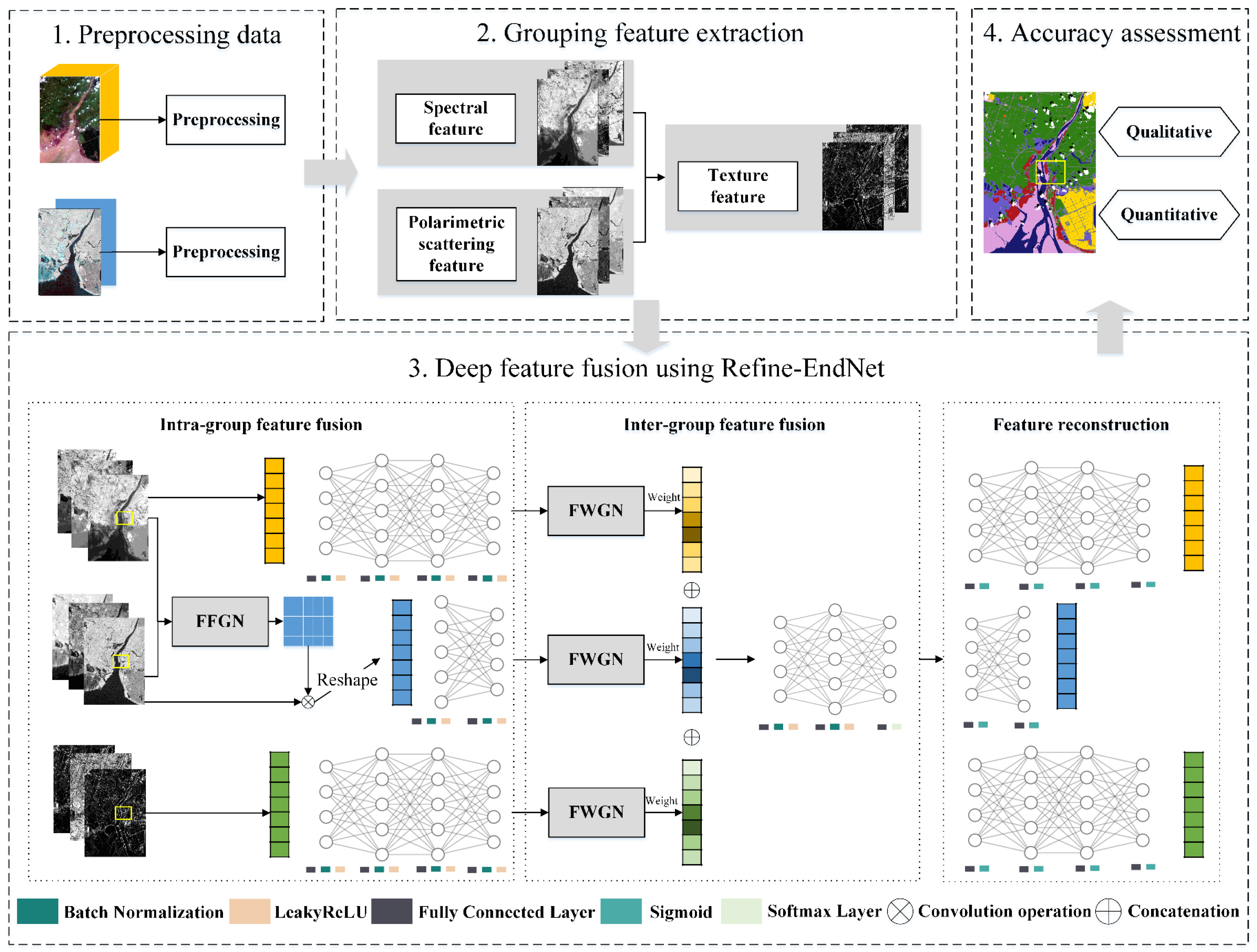
To solve the problems in the above research methods, the encoder–decoder framework [30] is selected from the perspective of adapting to data sources. The fully connected neural network is more suitable for feature extraction or feature fusion of hyperspectral data due to its transformation in channel dimension, and more channel information can be retained [31]. However, the characteristics of SAR data and the fusion capacity of EndNet need to be further studied. The main objectives of this study were to:

• Propose a new encoder–decoder framework suitable for hyperspectral and SAR data;
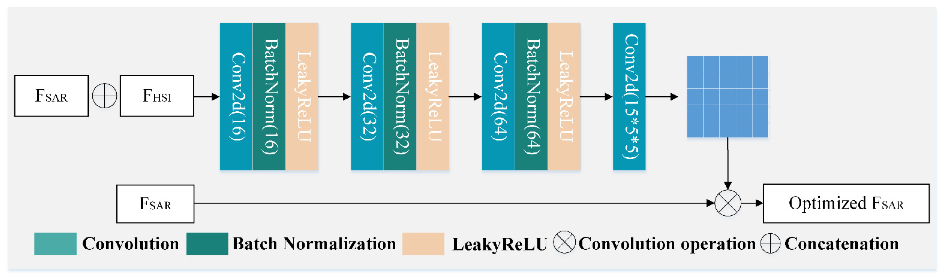
• Suppress the presence of speckle noise in SAR data and the heterogeneity between hyperspectral and SAR data on classification results by the fusion filter generation network (FFGN) based on a dynamic filtering network;
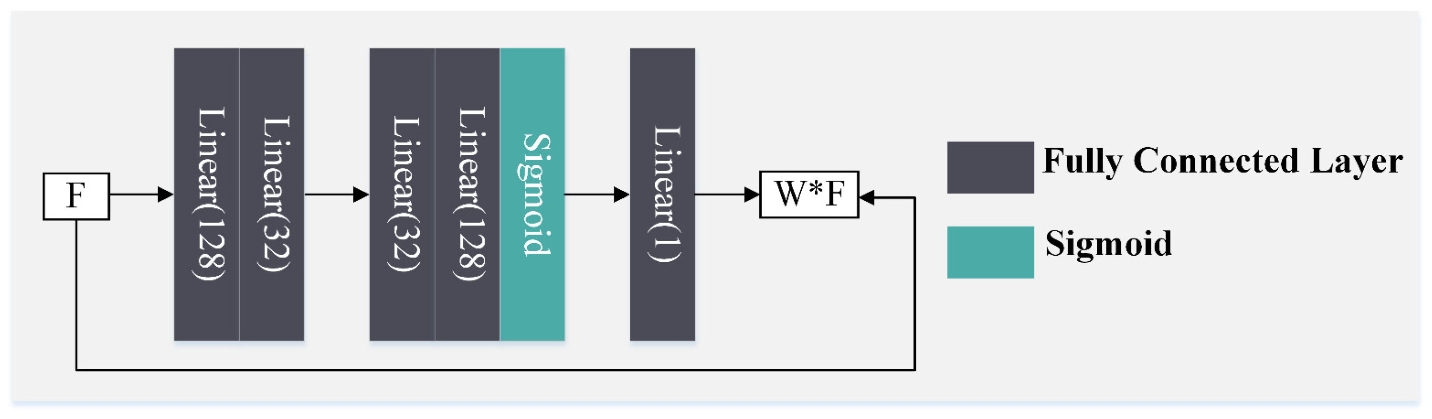
• Generate the fusion weight of group features to optimize the inter-group fusion process and improve the ability of fusion by the fusion weight generation network (FWGN) based on an attention mechanism.
• Improve the efficiency and accuracy of the algorithm by extracting feature information (spectral feature, texture feature, and polarization scattering feature) of ground objects from hyperspectral and SAR data and carrying out intra-group fusion.

The rest of this paper is organized as follows. In Section 2, the details and motivations of our proposed method are introduced. In Section 3, we show the experiments. Section 4 and Section 5 present the experimental results and discussion both qualitatively and quantitatively. Finally, Section 6 makes the summary with some important conclusions.

2. Materials and Methods

2.1. Overview

In this study, our proposed method follows an encoder–decoder framework that contains many fully connected neural networks. Figure 1 illustrates the flowchart of deep feature fusion using Refine-EndNet. Firstly, the spectral, texture, polarization, and scattering information are extracted from hyperspectral and SAR data that are preprocessed. Grouping these features and putting them into encoder layers that contain three branches separately, the intra-group feature is extracted deep abstract information and fused preliminarily by encoder layers in the feature dimension. The FFGN that follows a dynamic filter network is embedded into one of the branches to suppress the presence of speckle noise. Furthermore, the FWGN adds weight to optimize the grouping feature and combines the bottleneck to carry out inter-group feature fusion. The output of the bottleneck is the input of decoder layers and produces a label map. Lastly, the label map is evaluated from qualitative and quantitative aspects.

2.2. The Fusion Filter Generation Network

The dynamic filter network dynamically generates a filter based on input data, which has adaptability and flexibility and can realize local space conversion and adaptive feature extraction [32]. The generated dynamic filter does not share the weight among all pixels in the image, which is different from the standard convolution filter. Xu et al. believed that combining a dynamic filter network could effectively reduce the influence of speckle noise in SAR images [33]. Accordingly, hyperspectral $F_{HSI}\in {\mathbb{R}}^{h\times w\times c1}$ and SAR data $F_{SAR}\in {\mathbb{R}}^{h\times w\times c2}$ are concatenated together in feature dimension ($F_{HSI},F_{SAR})\in {\mathbb{R}}^{h\times w\times (c1+C2)}$, which is token as input. Pre-fusion is carried out through a dynamic filter network to realize the information interaction. Figure 2 illustrates the details of FFGN. In Figure 2, the fusion filter $\mathcal{F}\in {\mathbb{R}}^{h\times w\times c2\ast k^2}$ is generated by a dynamic filter network, wherein $k=5$, and it is reshaped into a dynamic convolution filter with a size of 5 $\times$ 5. As shown in Equation (1), keep convolution operation with each pixel position of $F_{SAR}\in {\mathbb{R}}^{h\times w\times c2}$ to optimize SAR data, and reduce the impact of heterogeneity with hyperspectral data.

$${Optimized F}_{SAR}=\mathcal{F}\otimes F_{SAR}$$

(1)

Note: ⊗ represents the convolution operation.

2.3. Deep Feature Fusion Using Refine-EndNet

MDL-RS is a sort of multimodal deep learning with a focus on remote sensing image classification, which contains two different forms: pixel-wise and spatial-spectral architectures designed by FC-Nets and CNNs [26]. As one of the MDL-RS methods consists of a feature extraction network (FE-Net), a fusion network (F-Network), and a Reconstruction Network (R-Net) [30]. In this study, an intra-group and inter-group feature fusion strategy is combined with EndNet. It is transformed into the Refine-EndNet, which comprises intra-group feature fusion, inter-group feature fusion, and feature reconstruction to realize deep feature fusion.

2.3.1. Intra-Group Feature Fusion

In the intra-group feature fusion, the spectral feature $F_1\in {\mathbb{R}}^{N\times c1}$, polarization decomposition and scattering feature $F_2\in {\mathbb{R}}^{N\times c2}$, and texture feature $F_3\in {\mathbb{R}}^{N\times c3}$ are fused through the three branches of FC-Nets of Refine-EndNet, respectively. $c1,c2,$ and $c3$ represent the dimensions of N pixels in the three groups of features. The intra-group feature fusion process is shown as follows:

$$z_{s,i}^{\left(l\right)}=\left\{\begin{array}{c}f\left(W_s^{\left(l\right)}{F}_{s,i}+b_s^{\left(l\right)}\right),l=1\\ f\left(W_s^{\left(l\right)}{F}_{s,i}^{\left(l-1\right)}+b_s^{\left(l\right)}\right),l=2,\cdots ,p\end{array}\right.$$

(2)

where $z_{s,i}^{\left(l\right)}$ is the fused intra-group feature for the $i$th pixel in the $l$th layer, $s$ stands for different grouping features; $f\left(·\right)$ is the non-linear activation function; $W_s^{\left(l\right)}$ and $b_s^{\left(l\right)}$ are the weights and biases of a grouping feature in the $l$th layer. A “block” of FC-Nets in this part consists of a fully connected (FC) layer, a batch normalization (BN) layer, and LeakyReLU activation layer.

2.3.2. Inter-Group Feature Fusion

To improve the fusion level of features after intra-group feature fusion, inter-group feature fusion is performed. $a_i$ is obtained from F-Net of EndNet [30] after equal weight fusion and the fusion process of F-Net is shown as Equation (3). Figure 3 illustrates the details of FWGN based on the attention mechanism. The fusion weight from FWGN is added to F-Net and it is transformed into a non-equal weight fusion process and is shown as Equation (4). During inter-group feature fusion, different weights are independent of each other, and not necessary for the sum to be 1. The greater the contribution to the classification results, the larger the weight.

$$a_i^{\left(l+1\right)}=h\left({[z}_{1,i}^{\left(l\right)}\oplus z_{2,i}^{\left(l\right)}\oplus z_{3,i}^{\left(l\right)}]\right)$$

(3)

$$a_i^{\left(l+1\right)}=h\left({[w_1\ast z}_{1,i}^{\left(l\right)}\oplus {w_2\ast z}_{2,i}^{\left(l\right)}\oplus {w_3\ast z}_{3,i}^{\left(l\right)}]\right)$$

(4)

where $a_i$ represents a feature from inter-group fusion; $h\left(·\right)$ is taken as a set of “blocks” that consists of the FC layer, the BN layer, and the LeakyReLU activation layer. ⊕ denotes a concatenation operator in the feature dimension. $w\in {ℝ}^{N\times 1}$ represents the weight that is given to each pixel in the spatial dimension.

2.3.3. Feature Reconstruction

In the feature reconstruction stage, the output feature map from inter-group feature fusion is directly transformed into original spectral, texture, polarization, and scattering features to preserve more useful information. The feature reconstruction process is shown as follows:

$$F_{s,i}=g\left(a_i^{\left(l+1\right)}\right), s=1, 2, 3$$

(5)

where $g\left(·\right)$ denotes the “block” that consists of the FC layer and the sigmoid activation layer. In particular, the reconstructed feature vector of the middle branch is similar to the SAR feature that is optimized by a fusion filter and reshaped into vector form.

2.3.4. Objective Function

In Equation (6), given the weight cross entropy and the mean square error between the encoding and decoding feature vectors as constraints.

$$\underset{\varnothing ,\phi }{\min }{{\displaystyle \sum }}_{s=1}^3\parallel F_s-g_{\phi }{\left(f_{\phi }\left(F_s\right)\right)\parallel }_F^2-\frac{1}{N}{{\displaystyle \sum }}_{i=1}^N\left[y_i\log a_i^{\left(l+1\right)}+\left(1-y_i\right)\log (1-a_i^{\left(l+1\right)})\right]$$

(6)

where $y_i$ is the label of the C category for each pixel.

3. Experiment Design

3.1. Study Area

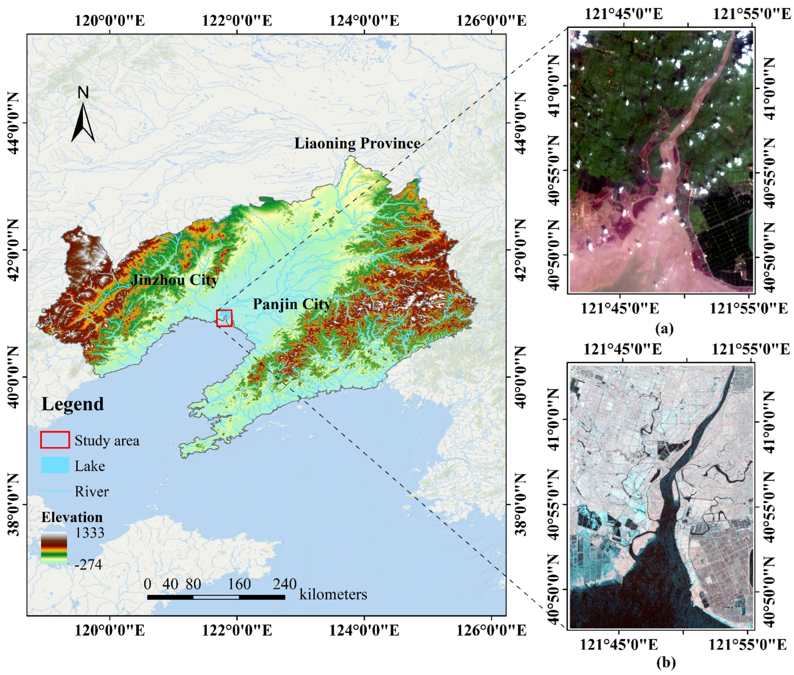
This study was carried in the Liao River Estuary National Nature Reserve in Panjin City, southern Liaoning Province, China, where the Liao River flows into the Bohai Sea (the red rectangle in Figure 4). The Liao River Estuary National Nature Reserve consists of the world’s largest reed marsh, a large area of suaeda community, and a shallow sea. The estuarine ecosystem provides a habitat for a variety of rare waterfowl, and the wetland landscape also provides good tourism resources for the local area. Figure 4 illustrates the geographic location of the study area. According to the standard of “Current land use classification” and the ground resolution of the ZY1-02D satellite hyperspectral data, the ground object category of the study area was determined. The sample statistics of the research area were verified by ZY1-02D satellite multispectral data and Google Earth high-resolution images (

Table 1. The sample information of the study area.

Class	Ground Objects	Number of Samples
C1	water	2168
C2	suaeda salt marsh	1682
C3	reed salt marsh	2614
C4	beach	4646
C5	paddy field	2096
C6	road and ditch	356
C7	aquiculture area	1935
C8	building area	269
C9	Oil well	125
C10	shadow	521
C11	cloud	2316

).

3.2. Hyperspectral and SAR Data and Preprocessing

The ZY1-02D satellite was launched on 12 September 2019, and fully inherits the advanced Gaofen−5 hyperspectral sensor technology to serve the monitoring of natural resources. It mainly carries two types of payloads, a visible, a near-infrared camera and an advanced hyperspectral imager sensor (AHSI) [7]. It covers 166 spectral bands ranging from 400 nm to 2500 nm. The spectral resolution of the visible and near-infrared band (VNIR) is 10 nm, the spectral resolution of the short-wave infrared band (SWIR) is 20 nm, and the spatial resolution is 30 m. The SAR data are an interferometric wide (IW) swath mode collected by Sentinel-1A with a spatial resolution of 5 × 20 m, which includes two polarization modes, namely vertical transmission vertical reception (VV) and vertical transmission horizontal reception (VH). Details of sensor parameters for hyperspectral and SAR data are shown in

Table 2. The information of AHSI on ZY1-02D and Sentinel-1A satellite.

Hyperspectral Image		SAR Image
Sensor	ZY1−02D AHSI	Sensor	Sentinel−1A
Launch Time	12 September 2019	Launch Time	3 April 2014
Spatial Resolution	30 m	Spatial Resolution	5 × 20 m
Spectral Resolution	10 nm (VNIR), 20 nm (SWIR)	Wavelength	C
Spectral Range	400–2500 nm	Polarization	VV and VH
Acquisition time	18 August 2021	Acquisition time	12 August 2021

. Auxiliary data are land use/land cover survey results and 30 m resolution digital elevation model (DEM) data in the study area.

The preprocessing of hyperspectral data includes anomalous band removal, radiometric calibration, atmospheric correction, and orthographic correction. Firstly, the spectral overlapping bands (VN: 72–76, five bands in total) between visible and short-wave infrared are eliminated. Secondly, the bands (SW: 22–27, 48–59, 82–83, 20 bands in total) affected by the water vapor absorption interval of 1357–1442 nm, 1795–1980 nm, and 2366–2384 nm are eliminated. Lastly, the bands (SW: 88–90, three bands in total) with low signal-to-noise ratio were eliminated. Radiometric calibration, atmospheric correction using FLAASH (Fast Line-of-sight Atmospheric Analysis of Spectral Hypercubes atmospheric correction), and orthotropic correction were performed for the remaining 138 bands.

The preprocessing of SAR data includes multi-looked processing, filtering, geocoding, and radiometric calibration. Firstly, the single-look complex data were multi-looked with a range number of one looks in the azimuth and five in the range, resulting in a ground-range resolution of 18.47 $\times$ 13.89 m. The speckle noise was removed using the Frost filter with 5 $\times$5 windows. The VV and VH images were geocoded to World Geodetic System 1984 datum and Universal Transverse Mercator Zone 50 North coordinate system via Range–Doppler terrain correction using DEM data, then radiometric calibration was carried out. Finally, they were resampled to a 30 m spatial resolution and georeferenced with hyperspectral data with an error of fewer than 0.5 pixels. The preprocessed hyperspectral and SAR datasets with a size of 965 $\times$ 635 were obtained.

3.3. Grouping Feature Extraction

Feature extraction (spectral, texture, polarization, and scattering features) is carried out on the original hyperspectral and SAR data to: (1) reduce redundant information or enrich the feature information; (2) improve the ability of subsequent model learning and generalization; (3) highlight the representative information of the original data and obtain the feature representation with obvious physical significance and strong interpretation.

3.3.1. Spectral Feature

Spectral features can be divided into dimensionality reduction and spectral index features [17]. The first part includes the first three principal component features obtained by the principal component transformation of all spectral bands of the hyperspectral data, the first five band features obtained by the minimum noise transformation of all spectral bands, and the commonly used ρ12, ρ21, ρ33, ρ55, ρ102, ρ125 of a total of seven multispectral bands. It aims to remove redundant information while preserving the main information of the spectral band as much as possible. The second part (shown as

Table 3. The vegetation index (VI) features of ZY1−02D satellite hyperspectral data and their corresponding equations.

VI	Formulation
NDVI	$\mathrm{NDVI}=\left(\mathsf{\rho }{55}^{ 1}-\mathsf{\rho }33\right)/\left(\mathsf{\rho }55+\mathsf{\rho }33\right)$
NDWI	$\mathrm{NDWI}=\left(\mathsf{\rho }21-\mathsf{\rho }55\right)/\left(\mathsf{\rho }21+\mathsf{\rho }55\right)$
ARI2	$\mathrm{ARI}2=\mathsf{\rho }48\left(1/\mathsf{\rho }19-1/\mathsf{\rho }37\right)$
PRI	$\mathrm{PRI}=\left(\mathsf{\rho }{17}^{ 1}-\mathsf{\rho }21\right)/\left(\mathsf{\rho }17+\mathsf{\rho }21\right)$
TCARI	$\mathrm{TCARI}=3\left[\left(\mathsf{\rho }37-\mathsf{\rho }33\right)-0.2\left(\mathsf{\rho }37-\mathsf{\rho }19\right)\times \left(\mathsf{\rho }37/\mathsf{\rho }33\right)\right]$
OSAVI	$\mathrm{OSAVI}=\left(1+0.16\right)\times \left(\mathsf{\rho }48-\mathsf{\rho }33\right)/\left(\mathsf{\rho }48+\mathsf{\rho }33+0.16\right)$

¹ $\mathsf{\rho }17$ and $\mathsf{\rho }55$ represents the 17th and 55th bands of ZY1-02D satellite hyperspectral data.

) includes the Normalized Difference Vegetation Index (NDVI) [34], the Normalized Difference Water Index (NDWI) [35], the Anthocyanin Reflectance Index2 (ARI2) [36], the Photochemical Reflectance Index (PRI) [37], the Transformed Chlorophyll Absorption in Reflectance Index (TCARI), and the Optimized Soil-Adjusted Vegetation Index (OSAVI) [38]. It aims to reflect information on canopy structure, pigmentation, leaf nitrogen content, and environmental humidity.

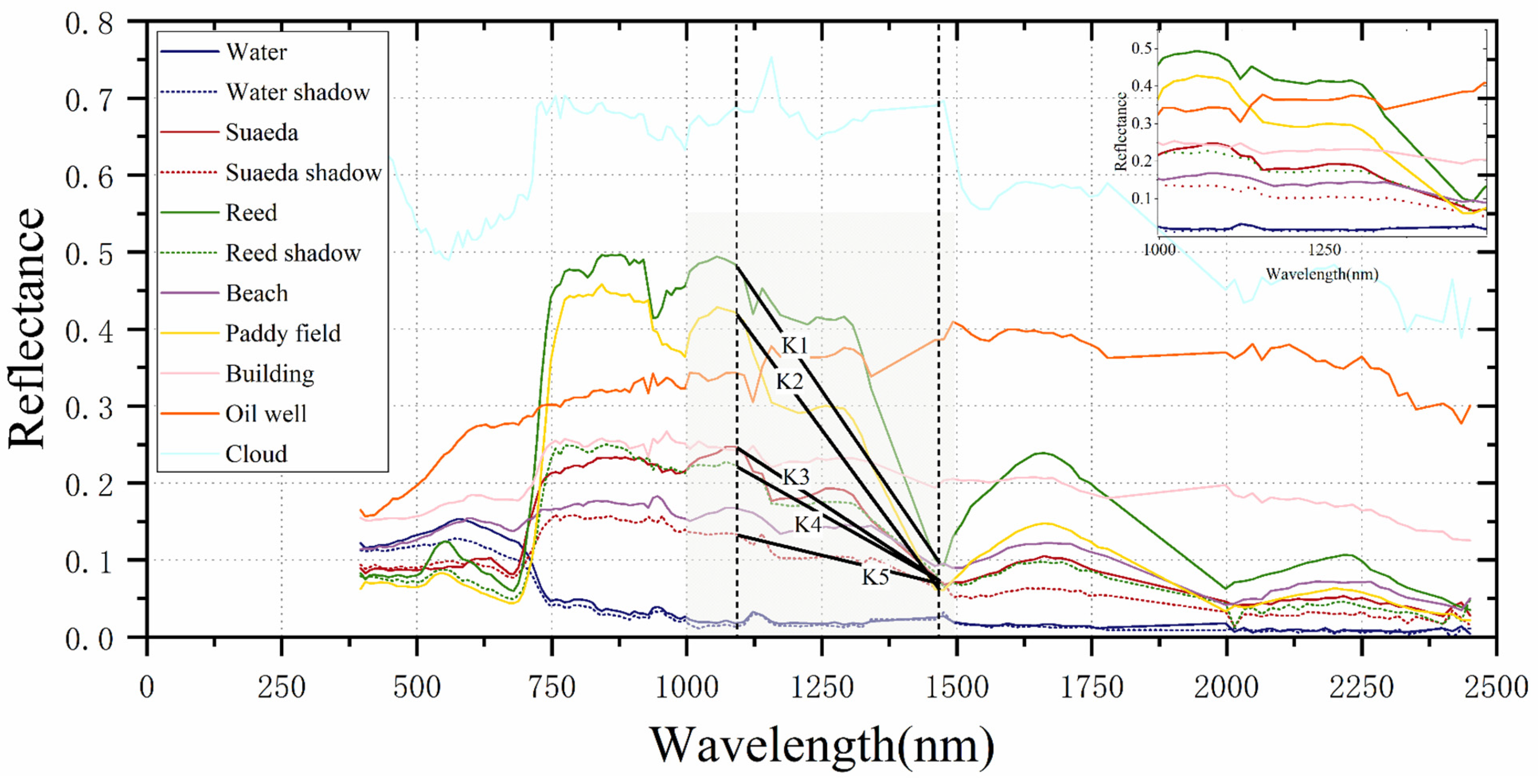
According to the rich geometric characteristics of the hyperspectral reflectance curve, the differences between vegetation under the shadows and vegetation in the bright area are further explored based on the NDVI, to improve the separability between the shadows and the salt marsh vegetation. Figure 5 illustrates the spectral characteristic curves of main land cover types in the study area, where the reflectance of vegetation under the shadows is much lower than the vegetation in the bright area at the near-infrared band. As shown in Figure 5, the reflectance of reed under the shadow is similar to suaeda in the bright area. Specially, the difference is greatest at 1089.23 nm and 1475.86 nm is the strong absorption position of all vegetation spectral curves. Therefore, the slope $K$ in these two spectral intervals can suppress vegetation information under shadows and highlight vegetation information in the bright area. Moreover, NDVI can effectively distinguish water from vegetation. In addition, slope $K$ can also effectively suppress non-vegetation objects such as buildings and clouds, while the red vegetation has the maximum reflectance in the red band. The hyperspectral shadow vegetation index (HSVI) Equation (7) is proposed to achieve reed > paddy field > suaeda > vegetation under the shadow. 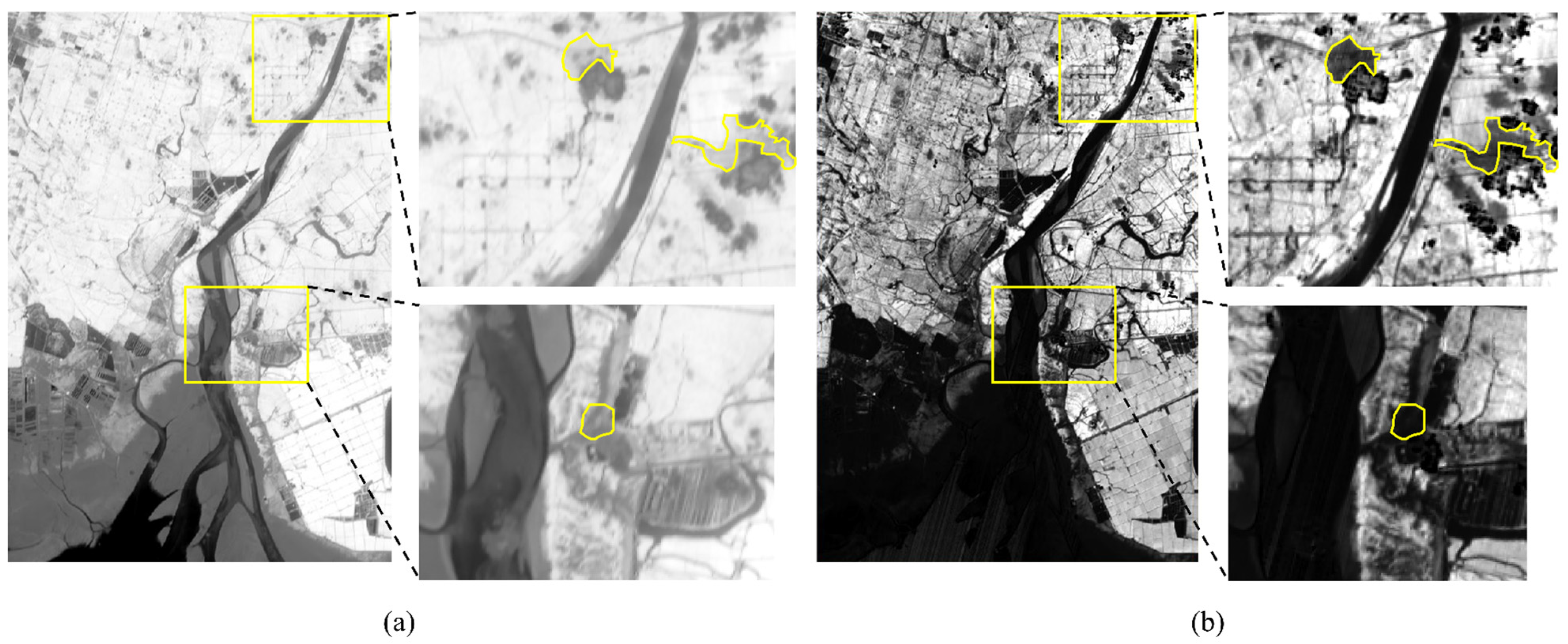Figure 6 shows the comparison between NDVI and the proposed index, which can effectively distinguish the three types of vegetation from the shadows.

$$HSVI=NDVI\ast K\ast \rho 29$$

(7)

3.3.2. Polarimetric Scattering Feature

The polarization scattering feature is used to represent the original SAR data, including matrix elements, polarization decomposition, and backscattering features (

Table 4. The partial polarization and scattering feature of dual-polarization SAR data and their corresponding equations.

Polarimetric Decomposition and Scattering Feature		Formulation
Matrix elements	$C_{11}$	${\left|S_{VV}\right|}^2$
	$C_{22}$	${\left|S_{VH}\right|}^2$
	Entropy ($H$)	$H=-{\displaystyle {\displaystyle \sum }_{i=1}^n}{P}_{i}lo{g}_2{P}_i$
Polarization decomposition	Anisotropy ($A$) *	$A=\frac{{\lambda }_1-{\lambda }_2}{{\lambda }_1+{\lambda }_2}$
	Alpha ($\alpha$) *	$\alpha ={\displaystyle {\displaystyle \sum }_{i=1}^n}{P}_i{\alpha }_i; {\alpha }_i=co{s}^{-1}\left(\left|v_{1i}\right|\right)$
	Pseudo probability ($P_1, P_2$)	$P_i=\frac{{\lambda }_i}{{{\displaystyle \sum }}_{j=1}^n{\lambda }_j}$
Backscattering	Cross-polarization ratio	$\frac{S_{VV}}{S_{VH}}$
	Cross-polarization difference	$S_{VV}-S_{VH}$

* ${\lambda }_i$ and $v$ represent the eigenvalue and eigenvector. For a more detailed description of the polarization decomposition features investigated in this study, interested readers can refer to [43].

). They are designed to reflect the different geometric and dielectric properties of ground objects [39,40,41,42]. The $H$-$A$-$\alpha$ decomposition method proposed by Cloude and Pottier is used to extract the eigenvalues and eigenvectors of dual-polarization (DP) SAR data by covariance matrix [$C$] Equation (8). $H$, $A$, $\alpha$, and eigenvalue parameters are calculated [43,44].

$$\left[C\right]=\left[\begin{array}{cc}\langle S_{VV}{S}_{VV}^{*}\rangle & \langle S_{VV}{S}_{VH}^{*}\rangle \\ \langle S_{VH}{S}_{VV}^{*}\rangle & \langle S_{VH}{S}_{VH}^{*}\rangle \end{array}\right]$$

(8)

where the matrix elements include $C_{11}$ and $C_{22}$, namely diagonal elements in the covariance matrix; the polarization decomposition feature includes Entropy ($H$), Anisotropy ($A$), Alpha ($\alpha$), eigenvector ($v$), Shannon Entropy ($SE$), Pseudo Probability ($P_1, P_2$) and Lambda (${\lambda }_1, {\lambda }_2$). The backscattering feature includes VV, VH, and the intensity information of cross-polarization ratio and cross-polarization difference.

3.3.3. Texture Feature

Although fully connected neural networks do not lose spatial information, local information reflected by texture features contributes significantly to classification accuracy [45]. Grey-Level Co-occurrence Matrix (GLCM) is a common method to extract texture features [5,18,36].

Table 5. The texture variables of the Grey-Level Co-occurrence Matrix (GLCM) and their corresponding equations using in this study.

Texture Variables	Formulation
Mean *	$Mean=\sum ip\left[i,j\right]$
Variance	$\mathrm{Variance}=\sum i^{2}p\left[i,j\right]-\sum ip\left[i,j\right]$
Homogeneity	$Homogeneity={\displaystyle {\displaystyle \sum }_i}{\displaystyle {\displaystyle \sum }_j}\frac{p\left[i,j\right]}{1+{\left(i-j\right)}^2}$
Contrast	$Contrast={\displaystyle {\displaystyle \sum }_i}{\displaystyle {\displaystyle \sum }_j}p{\left(i-j\right)}^{2}p\left[i,j\right]$
Dissimilarity	$\mathrm{Dissimilarity} ={\displaystyle {\displaystyle \sum }_i}{\displaystyle {\displaystyle \sum }_j}p\left|i,j\right|$
Correlation	$\mathrm{Correlation}=\frac{{{\displaystyle \sum }}_i{{\displaystyle \sum }}_{j}ijp\left[i,j\right]-\sum ip\left[i,j\right]\sum jp\left[i,j\right]}{\sqrt{\sum i^{2}p\left[i,j\right]-\sum ip\left[i,j\right]}\ast \sqrt{\sum j^{2}p\left[i,j\right]-\sum jp\left[i,j\right]}}$

* $i$, $j$ represents the sequence number of row and column pixels in the image, and $p\left[i,j\right]$ represents the relative frequency between two neighborhood pixels.

illustrates different variables that reflect the texture information in GLCM. Based on the principal component transformation of hyperspectral data, the first three principal components are selected to extract the texture features (mean, variance, heterogeneity, contrast, dissimilarity, and correlation). For SAR data, identical texture features are extracted based on backscattering features, matrix elements, and Shannon Entropy.

3.4. Experimental Setup

Experimental environment: the experiment was carried out on an Intel CPU with 2.30 GHz and 86 GB RAM. A NVIDIA GeForce RTX 3090 GPU with 24 GB of memory under CUDA version 11.3 was also employed. The deep learning framework is Pytorch1.11.0 in this study.

Experimental parameters: the proposed network was trained using the objective function mentioned earlier and an Adam optimizer [46] and a batch size of 64. The initialized learning rate was set to 0.001. The size of each FC layer was selected in the range of {16, 32, 64, 128, 256}, which is the same as EndNet. Moreover, the momentum is parameterized by 0.1. In intra-group feature fusion and feature reconstruction, the two branches that spectral feature and texture feature were input have four FC layers with the size of 16, 32, 64, and 128. More specifically, one of the branches that polarization and scattering feature was input comprised two FC layers with the size of 64 and 128. Settings above were aimed to keep the feature dimensions of the three branch networks the same. The influences of hyperparameters such as epoch, patch size, and Convolution kernel size of Refine-EndNet on classification accuracy were discussed in detail in the following sections.

Evaluation indexes: the classification performance of Refine-EndNet and other MDL methods were quantitatively evaluated by overall accuracy (OA), average accuracy (AA), and Kappa coefficient. Their visual effects of them were qualitatively evaluated.

3.5. Comparison of Experimental Parameters

3.5.1. Epoch of Refine-EndNet

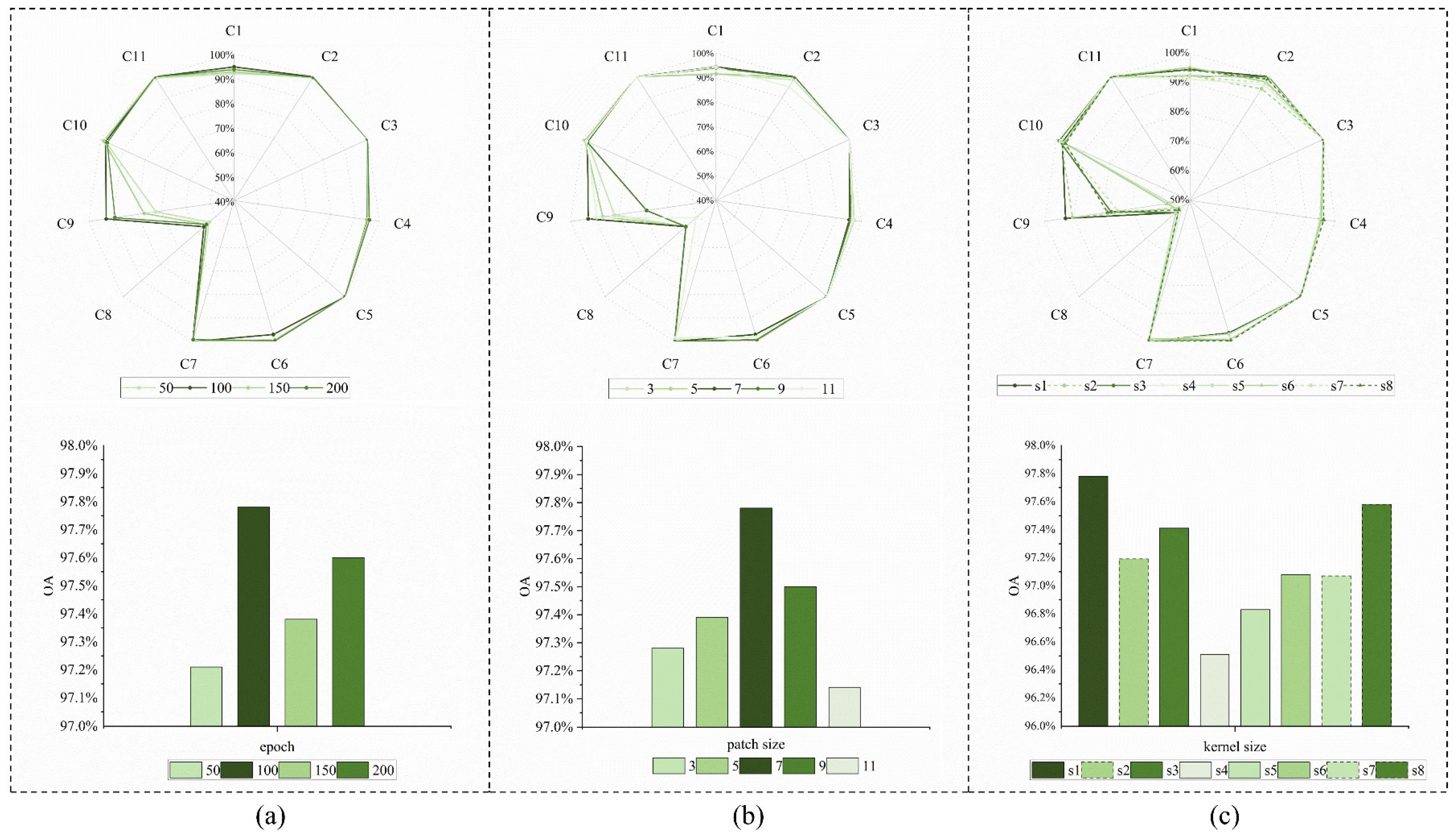
For Refine-EndNet, Figure 7a demonstrates the influence of the epoch on the classification accuracy, which compares the overall classification accuracy of 50, 100, 150, and 200 epochs. Overall, they are all between 97% and 98%, and the result of 100 epochs at 97.78% is the best.

3.5.2. Patch Size of Refine-EndNet

Figure 7a,b illustrates the impact of the different patch sizes on classification accuracy. With the gradual increase in patch size, the classification accuracy increases first and then decreases, and the overall accuracy is between 97% and 98%. The FFGN is used for pre-fusion hyperspectral and SAR data, for different categories of ground objects, and the classification accuracy is highest with the patch size of 7 × 7.

3.5.3. Convolution Kernel Size of Refine-EndNet

Figure 7c illustrates the influence of strategies with various convolution kernel sizes on the classification accuracy for Refine-EndNet. There are a total of eight strategies identified, numbered S1 to S8. S1 represented the size of the convolution kernel as 1 × 1, S2 represented 3 × 3, S3 represented 5 × 5, S4 represented 7 × 7, S5 represented 3 × 3 and 1 × 1, S6 represented 1 × 1 and 3 × 3, S7 represented 5 × 5 and 1 × 1, and S8 represented 1 × 1 and 5 × 5. The overall classification accuracy of S1 and S8 is the highest. For the oil well, S1 has a higher classification accuracy than S8.

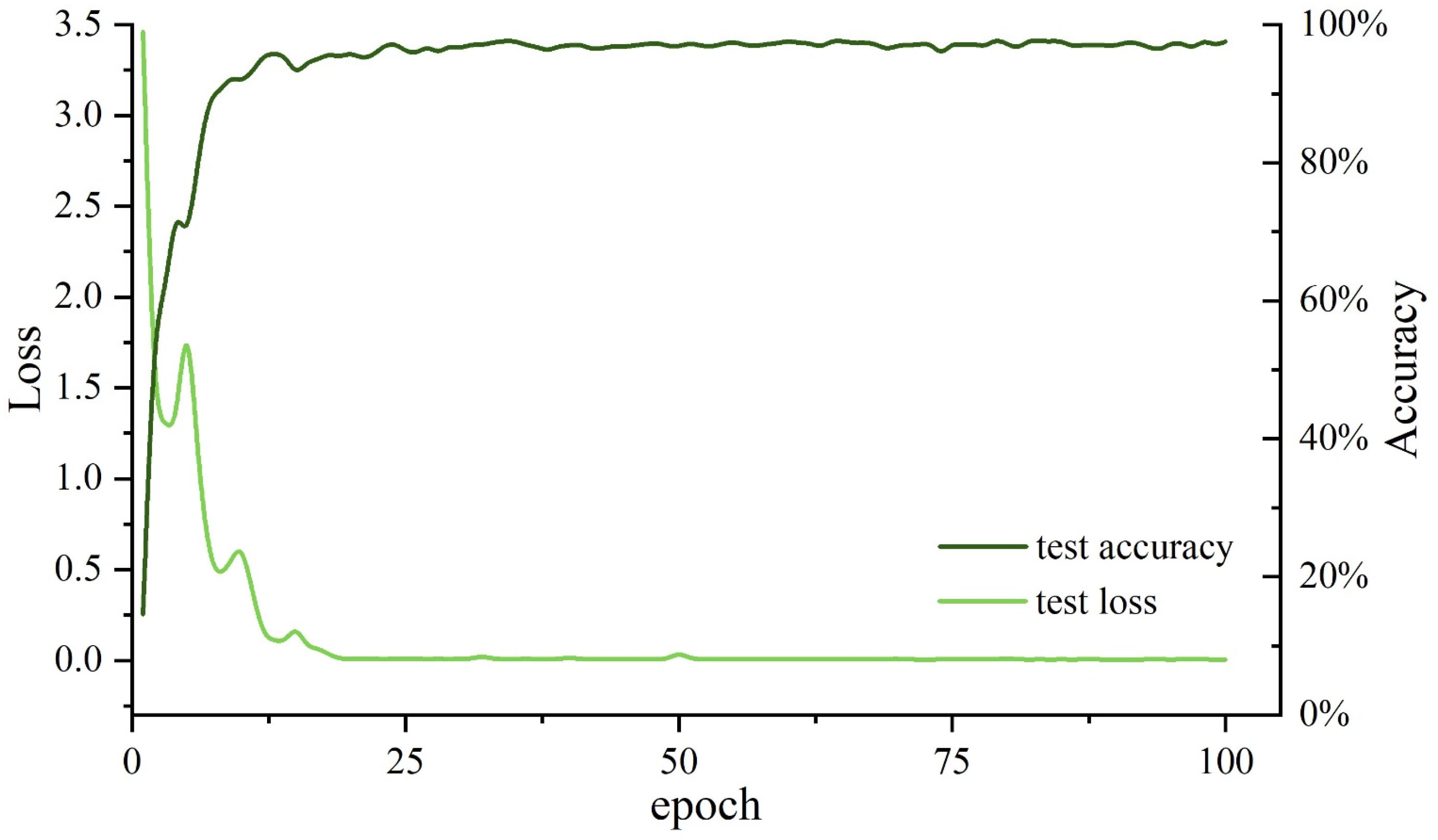
Overall, we select the epochs of 100, a patch size of 7 × 7, and a convolution kernel size of 1 × 1 as hyperparameters to train our proposed deep feature fusion model. The training curves consist of test loss and test accuracy are shown in Figure 8.

4. Results

4.1. Ablation Experiment

To measure the improvement of the EndNet by three parts: feature grouping (FG), FFGN, and FWGN, three ablation experiments were carried out in this study. In the first analysis, a branch network was added based on EndNet, and spectral, texture, polarization, and scattering features were used instead of the original image as input. Setting above makes the three-branch network more focused on the extraction and fusion of intra-group features. To accurately evaluate the effectiveness of FFGN and FWGN, only the part of FFGN was maintained in the second analysis. Finally, only the part of FWGN was maintained.

Table 6. Experimental results on the importance of feature grouping (FG), FFGN, and FWGN.

Baseline	FG	FFGN	FWGN	OA
■				95.12%
■	■			97.23%
■		■		96.79%
■			■	96.02%
■	■	■	■	97.78%

contains the comparison results of three ablation experiments, the baseline, and the proposed method.

Table 6 shows that FG, FFGN, and FWGN are all beneficial to improving the accuracy of ground object classification. The part of FG is more advantageous, and when this part exists in the model structure, the overall accuracy is improved by 2.11%. When the FFGN exists, the overall accuracy is improved by 1.67%. When the FFGN is included in the model structure, the overall accuracy is improved by 0.90%.

Table 7. The training time (in seconds) of 100 epochs for training different methods.

Methods	EndNet-FC	EndNet-CNN	FusAtNet	S2Enet	Refine-EndNet
time	365	496	--	385	404

represents the training time of 100 epochs for training different methods in this study. Refine-EndNet exhibits a slightly slower convergence than the EndNet-FC and S2ENet, given its relatively complex framework. FusAtNet was out of memory in the same experimental environment. Refine-EndNet performs a faster convergence than the EndNet-CNN and FusAtNet.

4.2. Feature Visualization

The fusion feature is visualized to investigate the effect of our proposed method. As shown in Figure 9, we select 16 representative feature maps of inter-group features with 128 dimensions. They have different emphases, which can be roughly divided in-to three aspects. Numbers 1, 18, 26, 55, 85, and 103 focus on the special characteristics of single or similar ground objects. Numbers 8, 36, 40, 67, 72, 91, and 116 concentrate on the information of ground object details. Numbers 11, 61, and 117 focus on the identification of texture information of ground objects. All feature maps include clouds and shadows without speckle noise. Therefore, the heterogeneity of hyperspectral and SAR data is well eliminated, and the influence of speckle noise on ground object classification is suppressed. The spectral, texture, polarization, and scattering information de-rived from the two multimodal data sources are used comprehensively, and the abstract information representation is generated.

The separability of different ground objects in Liao River Estuary National Nature Reserve under the grouping of spectral, texture, polarization, scattering features, and fusion features is visualized by the T-NSE algorithm [47] (shown in Figure 10). Among them, the different categories under fusion features can be distinguished best, and the sample points of the same category are clustered closely relative to the different categories under spectral features, polarization scattering features, and texture features. Therefore, our proposed method can improve the separability between the categories of ground objects.

4.3. Classification Results

Table 8. Classification results of the study area from different methods.

	EndNet-FC	EndNet-CNN	FusAtNet	S2ENet	R-EndNet2	FLIF-SVM	R-EndNe3
C1	93.15%	87.95%	89.73%	92.47%	92.33%	89.59%	94.52%
C2	98.98%	92.86%	96.53%	96.94%	96.33%	95.31%	100.00%
C3	99.88%	100.00%	99.88%	100.00%	100.00%	98.14%	100.00%
C4	99.00%	97.84%	93.01%	99.50%	96.84%	95.67%	95.01%
C5	95.48%	97.57%	97.57%	98.96%	100.00%	100.00%	100.00%
C6	98.86%	97.73%	87.88%	93.18%	98.86%	85.61%	96.97%
C7	92.69%	98.51%	97.65%	98.51%	97.03%	99.38%	100.00%
C8	54.93%	56.34%	56.34%	56.34%	46.48%	49.30%	56.34%
C9	95.18%	97.59%	71.08%	59.04%	98.80%	93.98%	92.77%
C10	69.58%	87.45%	87.45%	93.92%	95.06%	97.72%	97.72%
C11	100.00%	100.00%	100.00%	100.00%	100.00%	99.68%	100.00%
OA	95.14%	95.71%	94.71%	96.51%	96.84%	95.74%	97.78%
AA	90.70%	92.17%	88.83%	89.90%	92.88%	91.31%	93.94%
Kappa	0.9449	0.9513	0.9400	0.9604	0.9642	0.9517	0.9748

contains the comparison results of the quantitative evaluation indexes of EndNets [26], FusAtNet [28], S²ENet [29], FLIF-SVM, and Refined-EndNet. The FLIF-SVM is a conventional feature-level image fusion method that stacks features before sending them to the SVM. As shown in Table 8, the classification accuracy of all models except FusAtNet exceeds 95%. As aforementioned, FusAtNet and S²ENet are relatively superior models in MDL. When the original image is used as input, the overall classification accuracy of S²ENet achieves 96.51%, while that of FusAtNet is 94.71%, which is approximately 1% higher and 1% lower than that of EndNets, respectively. Refine-EndNet (R-EndNet2) outperform them with an overall accuracy of 96.84%, an average accuracy of 92.88%, and a Kappa coefficient of 0.9642. When the grouping features are used as inputs, Refine-EndNet (R-EndNet3) outperforms all methods with the highest overall classification accuracy of approximately 98%, an average accuracy of 93.94%, and the Kappa coefficient of 0.9748, suggesting an improvement of approximately 2.04% and 2.64% relative to the FLIF-SVM and EndNets, respectively. In summary, the evaluation indexes of Refine-EndNet are the most accurate among all models, regardless of whether the original images or the group features are used as inputs. It is more suitable for hyperspectral and SAR data fusion and has advantages in the task of ground object classification. All methods had the lowest accuracy of building land, possibly due to the relatively small number of training samples in this category.

Figure 11 demonstrates the comparison of classification effects of different methods in this study. As shown in Figure 11a,e,g, from the perspective of the overall visual effect, due to the injection of hyperspectral information and consideration of context information, the fusion of hyperspectral and SAR data through the encoder–decoder framework can suppress the speckle noise existing in SAR data to a certain extent. The injection of backscattered information also improves the separability of hyperspectral data between water and vegetation. In terms of local visual effects, the classification map obtained from EndNets is the poorest in complex scenes due to the limited fusion capacity, but the details of ground objects are maintained well (as shown in the first line in Figure 12). FusAtNet and S²ENet have poor classification effects in areas with dense shadows of cloud (as shown in the second line in Figure 12), and cannot effectively distinguish between water bodies and shadows (as shown in the third line in Figure 12). The FLIF-SVM had the worst classification map in the mixed growth area of reed and suaeda, and could not effectively identify water bodies (as shown in the second and third lines of Figure 12). Refine-EndNet maintains the ability of EndNet-FC that can distinguish the details of ground objects while achieving an excellent classification map in complex scenes, especially in areas where reeds and suaeda, water, and shadows mix and intervein.

5. Discussion

5.1. Effects of Cloud and Shadow for LULC Classification Using Hyperspectral and SAR

The revisit period of hyperspectral satellites is long, and the coastal region has cloudy coverage due to its climatic characteristics. So thick clouds and shadows become significant interference factors in the LULC classification of hyperspectral data, especially in areas with dense thick clouds and shadows. Previous studies have demonstrated the application potential of SAR data in water boundaries and vegetation extraction, which is not affected by clouds [10,14]. In this study, we found that hyperspectral data significantly contribute to the classification of ground objects. The previous studies combine SAR data to compensate for complex ground objects information under thick cloud and shadow [33,48,49]. If the same strategy is employed as in previous studies, the heterogeneity between multimodal data will lead to an unsatisfactory image reconstruction effect. Most of them are suitable for multispectral data, not for hyperspectral data. Therefore, clouds and shadows are included in the classification task as ground objects in this study.

Figure 13 demonstrates the normalized confusion matrix of the MDL approaches that contain EndNet-FC, FusAtNet, S²ENet, and the proposed method. All the methods achieve effective identification because the thick cloud has distinctive spectral curve characteristics. The shadow still has the spectral curve properties of the ground objects at the location, so it will inevitably emerge the error pixels. In the classification results of EndNet and FusAtNet, there are error pixels among shadow, water body, suaeda, and reed. As for S²ENet, there are considerably fewer error pixels among shadow, water body, and suaeda, relatively. As illustrated in Figure 13d, Refine-EndNet has the highest accuracy of shadow identification and the fewest error pixels. However, there are still error pixels with the suaeda and aquiculture areas.

5.2. Benefits of Refine-EndNet for Hyperspectral and SAR

5.2.1. Feature Engineering (FE) and Multimodal Deep Learning (MDL)

In this study, FE and MDL were combined to construct a deep feature fusion method. We found through experimental comparison (see Table 8) that extracting derived features of ground objects for the study area from the original data as input is a feasible way to improve classification accuracy. Although the MDL method has a more powerful ability of nonlinear fitting, the upper limit of classification accuracy still depends on the input data. This finding also explains that the research mode of “feature engineering + classifier” in FLIF is also applicable to deep learning. The efficiency and accuracy of the algorithm can be improved by artificially setting the feature information extracted from the branch network.

5.2.2. FFGN and FWGN

Hyperspectral and SAR data are multimodal remote sensing data. Moreover, hyperspectral data contain more additional information than SAR data due to the influence of cloud cover. It is impossible to perform effective feature fusion by directly inputting them into the encoder–decoder framework [30]. In this study, we found that the fusion level of complementary feature information can be enhanced by FFGN to achieve feature alignment through pre-fusion. Due to the injection of hyperspectral information, the speckle noise of SAR data is suppressed to some extent. As we all know, early, middle and late fusion [26] is equal weight fusion of multimodal data. The FWGN proposed in this study generates independent weights based on the grouping features themselves. It can optimize the contribution degree of feature information to classification results in the spatial dimension. The FFGN and FWGN guarantee that the addition of SAR data will not interfere with the classification effect of hyperspectral data on clouds and shadows (see Figure 13 and Table 8), and at the same time make proper use of the advantages of SAR data.

6. Conclusions

The accuracy of ground object classification is guaranteed by the complete fusion of complementary information from multimodal remote sensing data. In this study, a deep feature fusion method that follows an encoder–decoder framework is proposed for adapting hyperspectral and SAR data. It has two main components that aim to fully fuse spectral, texture, polarization, and scattering information and suppress the heterogeneity between hyperspectral and SAR data.

(1)

Intra-group feature fusion: Grouping features are optimized and fused by multi-branched fully connected neural networks, particularly for spectral information of hyperspectral data. Furthermore, the FFGN is utilized for pre-fusion to directly align the features of multimodal remote sensing data. It can effectively suppress the speckle noise of SAR data and the heterogeneity between hyperspectral and SAR data. However, the information of clouds and shadows are also brought into SAR data.

(2)

Inter-group feature fusion: The FWGN added independent weights in the spatial dimension to assess the importance and contribution of information from encoder layers for classification results and enhanced fusion capacity.

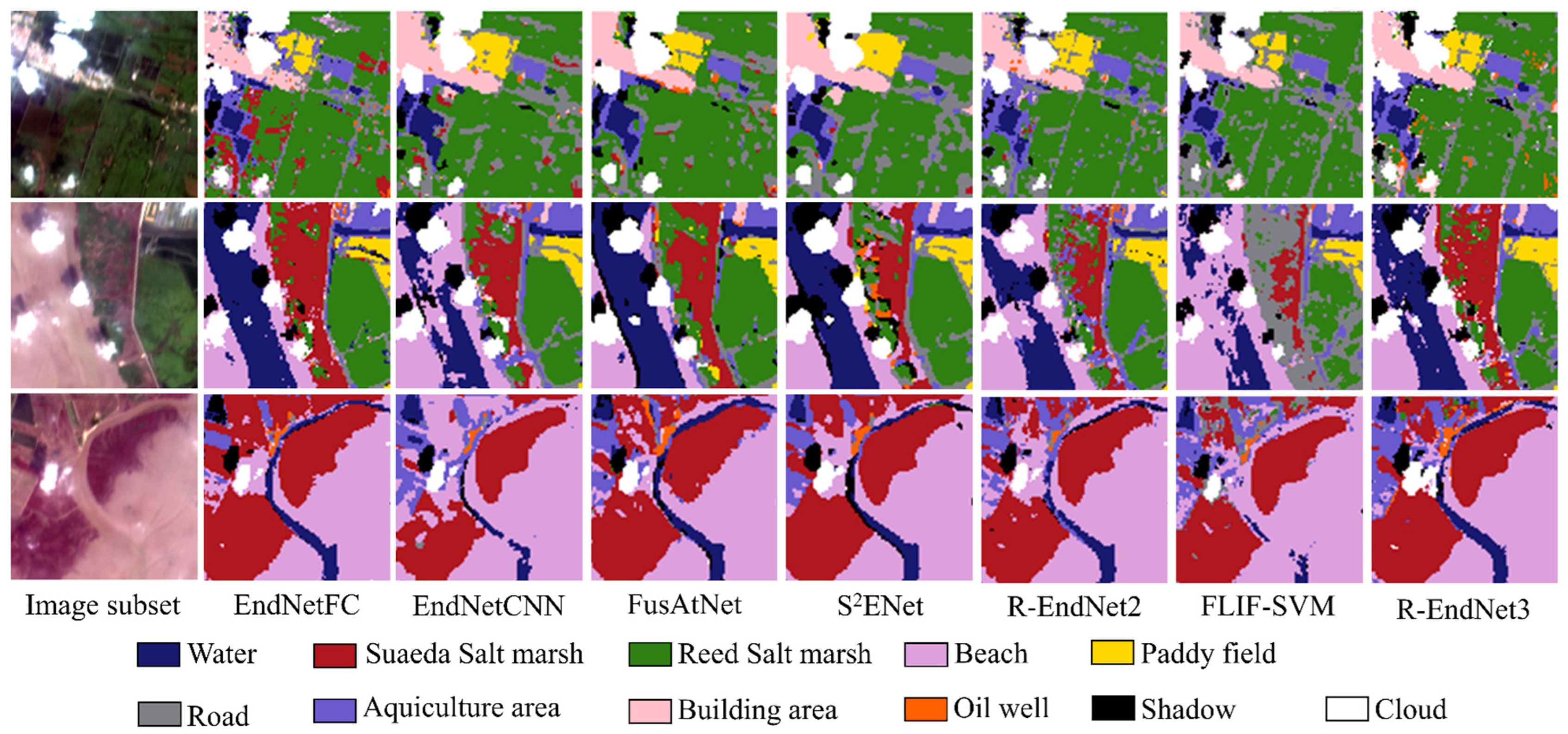
Our proposed method achieved a competitive classification accuracy of approximately 97.78%, providing an improvement of approximately 2.64% and 1.27% relative to EndNets and S²ENet, respectively. Although EndNet, FusAtNet, and S²ENet illustrated relatively equal strengths for fusing multimodal remote sensing data, Refine-EndNet is more advantageous for fusing hyperspectral and SAR data, particularly for hyperspectral data that are affected by clouds and shadows. Overall, our proposed method can realize the high-precision classification of ground objects and contribute to the deepening application of hyperspectral and SAR data.

References

1. Weiss, M.; Jacob, F.; Duveiller, G. Remote sensing for agricultural applications: A meta-review. Remote Sens. Environ. 2020, 236, 111402. [Google Scholar] [CrossRef]
2. Lary, D.J.; Alavi, A.H.; Gandomi, A.H.; Walker, A.L. Machine learning in geosciences and remote sensing. Geosci. Front. 2016, 7, 3–10. [Google Scholar] [CrossRef]
3. Wohlfart, C.; Winkler, K.; Wendleder, A.; Roth, A. TerraSAR-X and Wetlands: A Review. Remote Sens. 2018, 10, 916. [Google Scholar] [CrossRef]
4. Wang, W.; Yang, X.; Liu, G.; Zhou, H.; Ma, W.; Yu, Y.; Li, Z. Random Forest Classification of Sediments on Exposed Intertidal Flats Using Alos-2 Quad-Polarimetric Sar Data. ISPRS-Int. Arch. Photogramm. Remote Sens. Spat. Inf. Sci. 2016, XLI-B8, 1191–1194. [Google Scholar] [CrossRef]
5. Tu, C.; Li, P.; Li, Z.; Wang, H.; Yin, S.; Li, D.; Zhu, Q.; Chang, M.; Liu, J.; Wang, G. Synergetic Classification of Coastal Wetlands over the Yellow River Delta with GF-3 Full-Polarization SAR and Zhuhai-1 OHS Hyperspectral Remote Sensing. Remote Sens. 2021, 13, 4444. [Google Scholar] [CrossRef]
6. Jiao, L.; Sun, W.; Yang, G.; Ren, G.; Liu, Y. A Hierarchical Classification Framework of Satellite Multispectral/Hyperspectral Images for Mapping Coastal Wetlands. Remote Sens. 2019, 11, 2238. [Google Scholar] [CrossRef]
7. Sun, W.; Liu, K.; Ren, G.; Liu, W.; Yang, G.; Meng, X.; Peng, J. A simple and effective spectral-spatial method for mapping large-scale coastal wetlands using China ZY1-02D satellite hyperspectral images. Int. J. Appl. Earth Obs. Geoinf. 2021, 104, 102572. [Google Scholar] [CrossRef]
8. Gao, Y.; Song, X.; Li, W.; Wang, J.; He, J.; Jiang, X.; Feng, Y. Fusion Classification of HSI and MSI Using a Spatial-Spectral Vision Transformer for Wetland Biodiversity Estimation. Remote Sens. 2022, 14, 850. [Google Scholar] [CrossRef]
9. Liu, K.; Sun, W.; Shao, Y.; Liu, W.; Yang, G.; Meng, X.; Peng, J.; Mao, D.; Ren, K. Mapping Coastal Wetlands Using Transformer in Transformer Deep Network on China ZY1-02D Hyperspectral Satellite Images. IEEE J. Sel. Top. Appl. Earth Obs. Remote Sens. 2022, 15, 3891–3903. [Google Scholar] [CrossRef]
10. Horn, G.D.; Milne, A.K. Monitoring seasonal dynamics of northern Australian wetlands with multitemporal RADARSAT data. In Proceedings of the IEEE International Geoscience and Remote Sensing Symposium, Toronto, ON, Canada, 24–28 June 2002; pp. 137–139. [Google Scholar]
11. Mohammadimanesh, F.; Salehi, B.; Mahdianpari, M.; Homayouni, S. Unsupervised Wishart Classfication of Wetlands in Newfoundland, Canada Using Polsar Data Based on Fisher Linear Discriminant Analysis. ISPRS-Int. Arch. Photogramm. Remote Sens. Spat. Inf. Sci. 2016, XLI-B7, 305–310. [Google Scholar] [CrossRef]
12. Chatziantoniou, A.; Psomiadis, E.; Petropoulos, G. Co-Orbital Sentinel 1 and 2 for LULC Mapping with Emphasis on Wetlands in a Mediterranean Setting Based on Machine Learning. Remote Sens. 2017, 9, 1259. [Google Scholar] [CrossRef]
13. Koch, M.; Schmid, T.; Reyes, M.; Gumuzzio, J. Evaluating Full Polarimetric C- and L-Band Data for Mapping Wetland Conditions in a Semi-Arid Environment in Central Spain. IEEE J. Sel. Top. Appl. Earth Obs. Remote Sens. 2012, 5, 1033–1044. [Google Scholar] [CrossRef]
14. Zhang, X.; Xu, J.; Chen, Y.; Xu, K.; Wang, D. Coastal Wetland Classification with GF-3 Polarimetric SAR Imagery by Using Object-Oriented Random Forest Algorithm. Sensors 2021, 21, 3395. [Google Scholar] [CrossRef]
15. Mohammadimanesh, F.; Salehi, B.; Mahdianpari, M.; Gill, E.; Molinier, M. A new fully convolutional neural network for semantic segmentation of polarimetric SAR imagery in complex land cover ecosystem. ISPRS J. Photogramm. Remote Sens. 2019, 151, 223–236. [Google Scholar] [CrossRef]
16. Vali, A.; Comai, S.; Matteucci, M. Deep Learning for Land Use and Land Cover Classification Based on Hyperspectral and Multispectral Earth Observation Data: A Review. Remote Sens. 2020, 12, 2495. [Google Scholar] [CrossRef]
17. Bao, S.; Cao, C.; Chen, W.; Tian, H. Spectral features and separability of alpine wetland grass species. Spectrosc. Lett. 2016, 50, 245–256. [Google Scholar] [CrossRef]
18. Cao, J.; Leng, W.; Liu, K.; Liu, L.; He, Z.; Zhu, Y. Object-Based Mangrove Species Classification Using Unmanned Aerial Vehicle Hyperspectral Images and Digital Surface Models. Remote Sens. 2018, 10, 89. [Google Scholar] [CrossRef]
19. Abdel-Hamid, A.; Dubovyk, O.; Abou El-Magd, I.; Menz, G. Mapping Mangroves Extents on the Red Sea Coastline in Egypt using Polarimetric SAR and High Resolution Optical Remote Sensing Data. Sustainability 2018, 10, 646. [Google Scholar] [CrossRef]
20. Gao, Y.; Li, W.; Zhang, M.; Wang, J.; Sun, W.; Tao, R.; Du, Q. Hyperspectral and Multispectral Classification for Coastal Wetland Using Depthwise Feature Interaction Network. IEEE Trans. Geosci. Remote Sens. 2022, 60, 1–15. [Google Scholar] [CrossRef]
21. Rasti, B.; Hong, D.; Hang, R.; Ghamisi, P.; Kang, X.; Chanussot, J.; Benediktsson, J.A. Feature Extraction for Hyperspectral Imagery: The Evolution from Shallow to Deep: Overview and Toolbox. IEEE Geosci. Remote Sens. Mag. 2020, 8, 60–88. [Google Scholar] [CrossRef]
22. Wang, P.; Qiu, C.; Wang, J.; Wang, Y.; Tang, J.; Huang, B.; Su, J.; Zhang, Y. Multimodal Data Fusion Using Non-Sparse Multi-Kernel Learning with Regularized Label Softening. IEEE J. Sel. Top. Appl. Earth Obs. Remote Sens. 2021, 14, 6244–6252. [Google Scholar] [CrossRef]
23. Hu, J.; Hong, D.; Wang, Y.; Zhu, X. A Comparative Review of Manifold Learning Techniques for Hyperspectral and Polarimetric SAR Image Fusion. Remote Sens. 2019, 11, 681. [Google Scholar] [CrossRef]
24. Hong, D.; Hu, J.; Yao, J.; Chanussot, J.; Zhu, X.X. Multimodal remote sensing benchmark datasets for land cover classification with a shared and specific feature learning model. ISPRS J. Photogramm. Remote Sens. 2021, 178, 68–80. [Google Scholar] [CrossRef] [PubMed]
25. Rasti, B.; Ghamisi, P. Remote sensing image classification using subspace sensor fusion. Inf. Fusion 2020, 64, 121–130. [Google Scholar] [CrossRef]
26. Hong, D.; Gao, L.; Yokoya, N.; Yao, J.; Chanussot, J.; Du, Q.; Zhang, B. More Diverse Means Better: Multimodal Deep Learning Meets Remote-Sensing Imagery Classification. IEEE Trans. Geosci. Remote Sens. 2021, 59, 4340–4354. [Google Scholar] [CrossRef]
27. Wu, X.; Hong, D.; Chanussot, J. Convolutional Neural Networks for Multimodal Remote Sensing Data Classification. IEEE Trans. Geosci. Remote Sens. 2022, 60, 1–10. [Google Scholar] [CrossRef]
28. Mohla, S.; Pande, S.; Banerjee, B.; Chaudhuri, S. FusAtNet: Dual Attention based SpectroSpatial Multimodal Fusion Network for Hyperspectral and LiDAR Classification. In Proceedings of the 2020 IEEE/CVF Conference on Computer Vision and Pattern Recognition Workshops (CVPRW), Seattle, WA, USA, 14–19 June 2020; pp. 416–425. [Google Scholar]
29. Fang, S.; Li, K.; Li, Z. S²ENet: Spatial–Spectral Cross-Modal Enhancement Network for Classification of Hyperspectral and LiDAR Data. IEEE Geosci. Remote Sens. Lett. 2021, 19, 1–5. [Google Scholar] [CrossRef]
30. Hong, D.; Gao, L.; Hang, R.; Zhang, B.; Chanussot, J. Deep Encoder–Decoder Networks for Classification of Hyperspectral and LiDAR Data. IEEE Geosci. Remote Sens. Lett. 2020, 19, 1–5. [Google Scholar] [CrossRef]
31. Hong, D.; Yokoya, N.; Xia, G.S.; Chanussot, J.; Zhu, X.X. X-ModalNet: A semi-supervised deep cross-modal network for classification of remote sensing data. ISPRS J. Photogramm. Remote Sens. 2020, 167, 12–23. [Google Scholar] [CrossRef]
32. Jia, X.; De Brabandere, B.; Tuytelaars, T.; Gool, L.V. Dynamic filter networks. Adv. Neural Inf. Process. Syst. 2016, 29, 9673. [Google Scholar]
33. Xu, F.; Shi, Y.; Ebel, P.; Yu, L.; Xia, G.-S.; Yang, W.; Zhu, X.X. GLF-CR: SAR-enhanced cloud removal with global–local fusion. ISPRS J. Photogramm. Remote Sens. 2022, 192, 268–278. [Google Scholar] [CrossRef]
34. Sun, Y.; Ren, H.; Zhang, T.; Zhang, C.; Qin, Q. Crop Leaf Area Index Retrieval Based on Inverted Difference Vegetation Index and NDVI. IEEE Geosci. Remote Sens. Lett. 2018, 15, 1662–1666. [Google Scholar] [CrossRef]
35. Datt, B.; McVicar, T.R.; Van Niel, T.G.; Jupp, D.L.B.; Pearlman, J.S. Preprocessing eo-1 hyperion hyperspectral data to support the application of agricultural indexes. IEEE Trans. Geosci. Remote Sens. 2003, 41, 1246–1259. [Google Scholar] [CrossRef]
36. Chen, Y.; Tian, S. Feature-Level Fusion between Gaofen-5 and Sentinel-1A Data for Tea Plantation Mapping. Forests 2020, 11, 1357. [Google Scholar] [CrossRef]
37. Hernández-Clemente, R.; Navarro-Cerrillo, R.M.; Suárez, L.; Morales, F.; Zarco-Tejada, P.J. Assessing structural effects on PRI for stress detection in conifer forests. Remote Sens. Environ. 2011, 115, 2360–2375. [Google Scholar] [CrossRef]
38. Haboudane, D.; Miller, J.R.; Tremblay, N.; Zarco-Tejada, P.J.; Dextraze, L. Integrated narrow-band vegetation indices for prediction of crop chlorophyll content for application to precision agriculture. Remote Sens. Environ. 2002, 81, 416–426. [Google Scholar] [CrossRef]
39. Chen, Y.; He, X.; Xu, J.; Zhang, R.; Lu, Y. Scattering Feature Set Optimization and Polarimetric SAR Classification Using Object-Oriented RF-SFS Algorithm in Coastal Wetlands. Remote Sens. 2020, 12, 407. [Google Scholar] [CrossRef]
40. Gierszewska, M.; Berezowski, T. On the Role of Polarimetric Decomposition and Speckle Filtering Methods for C-Band SAR Wetland Classification Purposes. IEEE J. Sel. Top. Appl. Earth Obs. Remote Sens. 2022, 15, 2845–2860. [Google Scholar] [CrossRef]
41. Rapinel, S.; Betbeder, J.; Denize, J.; Fabre, E.; Pottier, É.; Hubert-Moy, L. SAR analysis of wetland ecosystems: Effects of band frequency, polarization mode and acquisition dates. ISPRS J. Photogramm. Remote Sens. 2020, 170, 103–113. [Google Scholar] [CrossRef]
42. Amani, M.; Salehi, B.; Mahdavi, S.; Brisco, B. Separability analysis of wetlands in Canada using multi-source SAR data. GISci. Remote Sens. 2019, 56, 1233–1260. [Google Scholar] [CrossRef]
43. Cloude, S.R.; Pottier, E. A review of target decomposition theorems in radar polarimetry. IEEE Trans. Geosci. Remote Sens. 1996, 34, 498–518. [Google Scholar] [CrossRef]
44. Harfenmeister, K.; Itzerott, S.; Weltzien, C.; Spengler, D. Agricultural Monitoring Using Polarimetric Decomposition Parameters of Sentinel-1 Data. Remote Sens. 2021, 13, 575. [Google Scholar] [CrossRef]
45. Zhang, C.; Selch, D.; Cooper, H. A Framework to Combine Three Remotely Sensed Data Sources for Vegetation Mapping in the Central Florida Everglades. Wetlands 2015, 36, 201–213. [Google Scholar] [CrossRef]
46. Kingma, D.P.; Ba, J. Adam: A method for stochastic optimization. arXiv 2014, arXiv:1412.6980. [Google Scholar]
47. Van der Maaten, L.; Hinton, G. Visualizing data using t-SNE. J. Mach. Learn. Res. 2008, 9, 2579–2605. [Google Scholar]
48. Meraner, A.; Ebel, P.; Zhu, X.X.; Schmitt, M. Cloud removal in Sentinel-2 imagery using a deep residual neural network and SAR-optical data fusion. ISPRS J. Photogramm. Remote Sens. 2020, 166, 333–346. [Google Scholar] [CrossRef] [PubMed]
49. Darbaghshahi, F.N.; Mohammadi, M.R.; Soryani, M. Cloud Removal in Remote Sensing Images Using Generative Adversarial Networks and SAR-to-Optical Image Translation. IEEE Trans. Geosci. Remote Sens. 2022, 60, 1–9. [Google Scholar] [CrossRef]
Figure 1. The flowchart of deep feature fusion using Refine-EndNet.
Land 12 01022 g001
Figure 2. Details of the fusion filter generation network (FFGN).
Land 12 01022 g002
Figure 3. Details of the fusion weight generation network (FWGN).
Land 12 01022 g003
Figure 4. Location of Panjin City, Liaoning Province in China, and the location of the study area: (a) the hyperspectral image (from Chinese ZY1−02D satellite, red = band 29; green = band 19; blue = band 10) and (b) the SAR image (from Sentinel−1A satellite, Pauli RGB) of the study area.
Land 12 01022 g004
Figure 5. Spectral characteristic curves of main land cover types in the study area.
Land 12 01022 g005
Figure 6. Comparison of the results between NDVI and the proposed index. (a) NDVI: the image calculated by the normalized difference between ρ 33 and ρ 55 . (b) HSVI: the image calculated by multiplying NDVI, ρ 29 , and the slope K .
Land 12 01022 g006
Figure 7. The comparison results of each category of classification accuracy and overall classification accuracy under different schemes: (a) comparison of different epochs, (b) comparison of different patch sizes, and (c) comparison of different convolution kernel sizes.
Land 12 01022 g007
Figure 8. The training curves of the proposed method.
Land 12 01022 g008
Figure 9. Visualized 16 of 128 output feature maps from the proposed method.
Land 12 01022 g009
Figure 10. Separability of 11 types of ground objects under: (a) spectral feature, (b) polarimetric and scattering feature, (c) texture feature, and (d) fusion feature.
Land 12 01022 g010
Figure 11. The classification maps were obtained from different methods: (a) EndNet-FC, (b) EndNet-CNN, (c) FusAtNet, (d) S2ENet, (e) R-EndNet2, (f) FLIF-SVM, and (g) R-EndNet3.
Land 12 01022 g011
Figure 12. The classification maps of three complex ground object regions in the study area from different methods.
Land 12 01022 g012
Figure 13. Normalized confusion matrices for ground object classification using (a) EndNet-FC, (b) FusAtNet, (c) S2ENet, and (d) Refine-EndNet.
Land 12 01022 g013