
Evaluating the Applicability of Global LULC Products and an Author-Generated Phenology-Based Map for Regional Analysis: A Case Study in Ecuador’s Ecoregions
 ,
,
Abstract
:1. Introduction
2. Materials and Methods
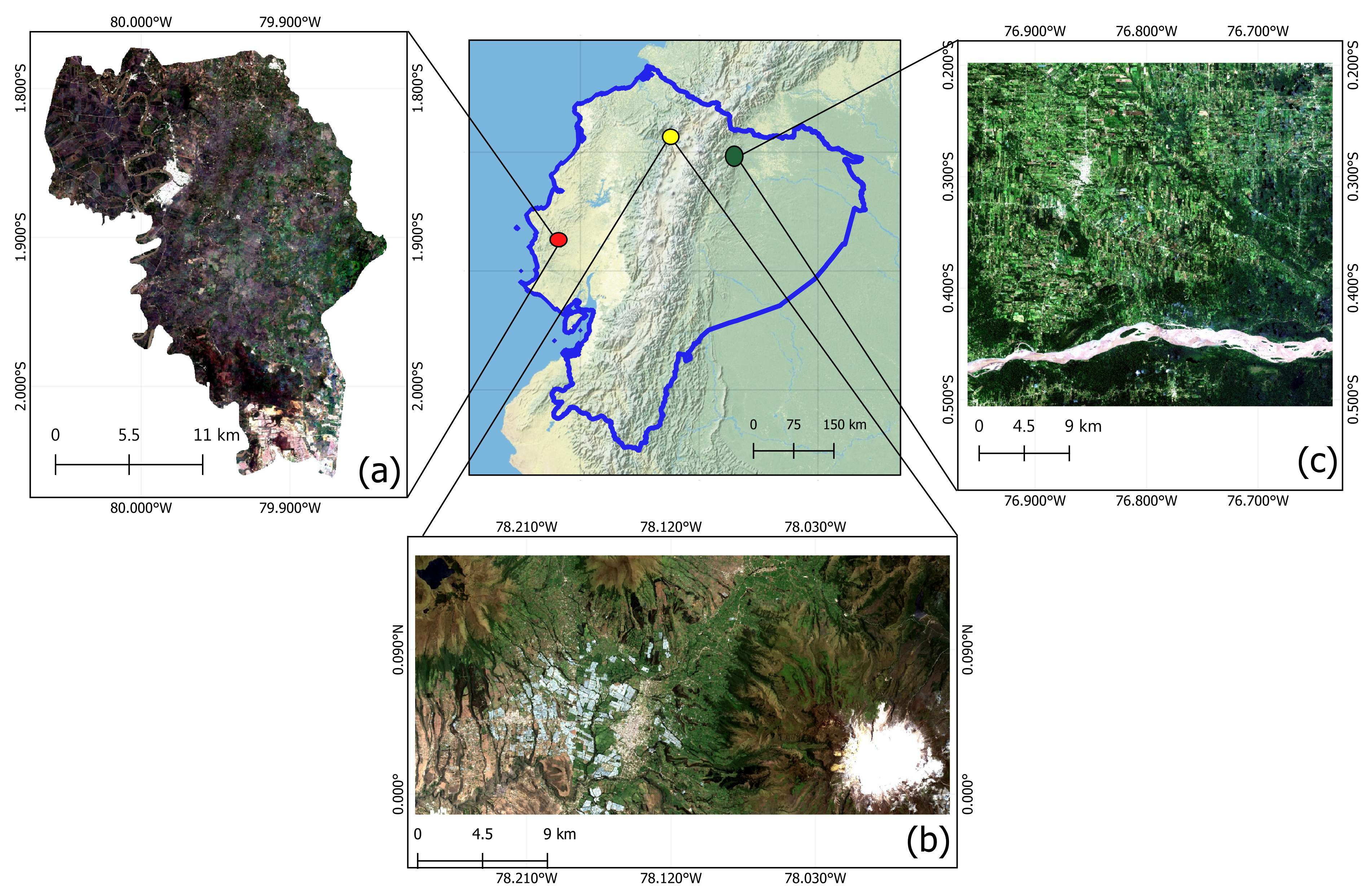
2.1. Target Areas
2.2. Datasets
2.3. Classification Scheme and Reference Data
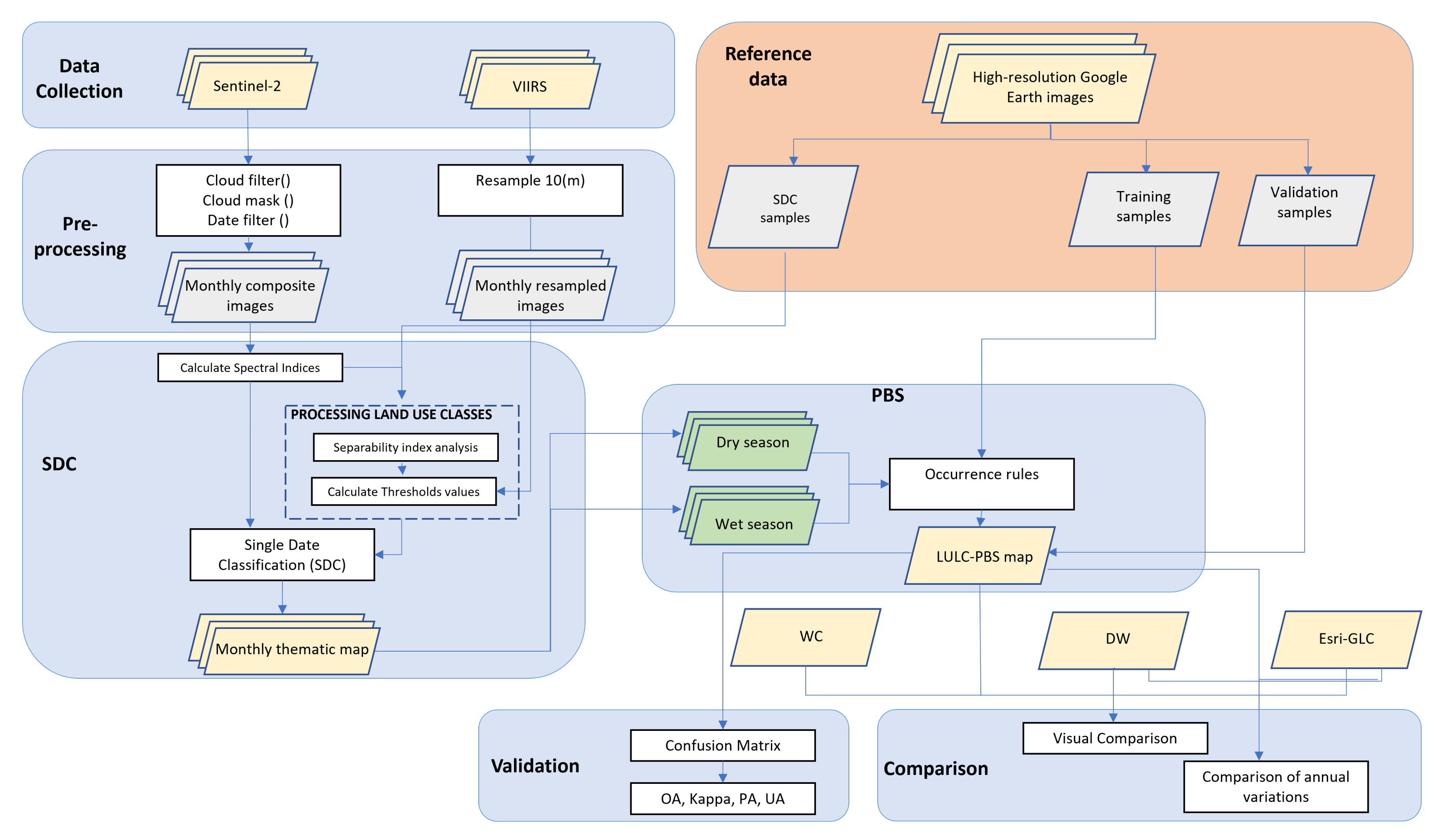
2.4. Methodology
2.4.1. SDC

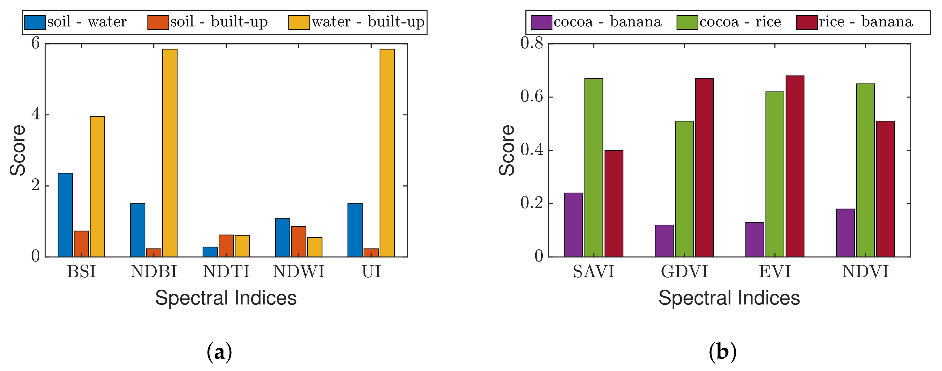
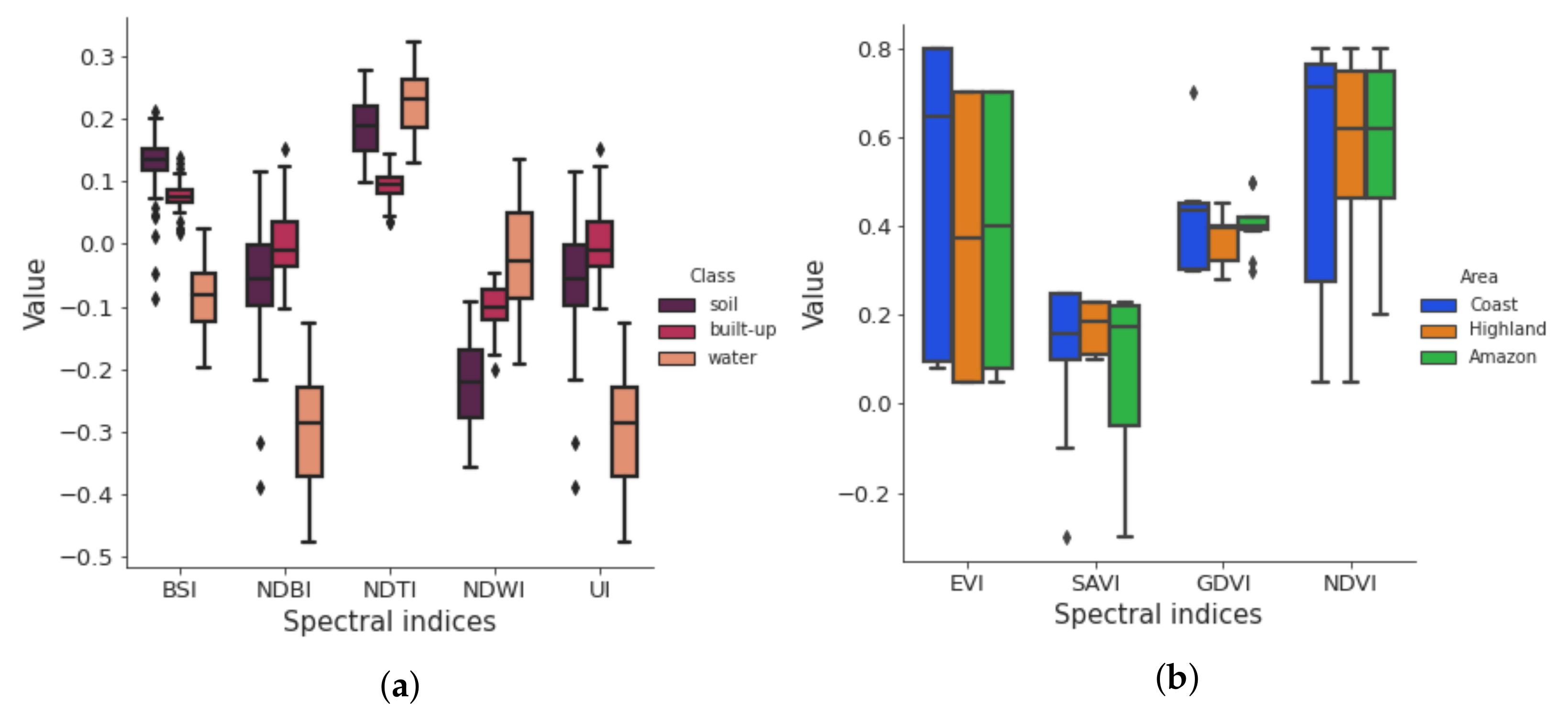
| Index | Equation | Ref. |
|---|---|---|
| Normalised difference vegetation index (NDVI) | [50] | |
| Bare soil index (BSI) | [51] | |
| Urban index (UI) | [52] | |
| Normalised difference built-up index (NDBI) | [53] | |
| Normalised difference tillage index (NDTI) | [54] | |
| Normalised difference water index (NDWI) | [55] | |
| Normalised difference snow index (NDSI) | [56] | |
| Green difference vegetation index (GDVI) | [57] | |
| Soil-adjusted vegetation index (SAVI) | [58] | |
| Enhanced vegetation index (EVI) | [59] |
2.4.2. PBS
2.4.3. Accuracy Metrics
2.4.4. LULC Maps Comparison
- , the name of a region: Coast C, Highlands H, or Amazon A.
- , a class in the set of the harmonised LULC classes, see Table 5.
- a given LULC map used for comparison.
- a year in the evaluation period.
3. Results
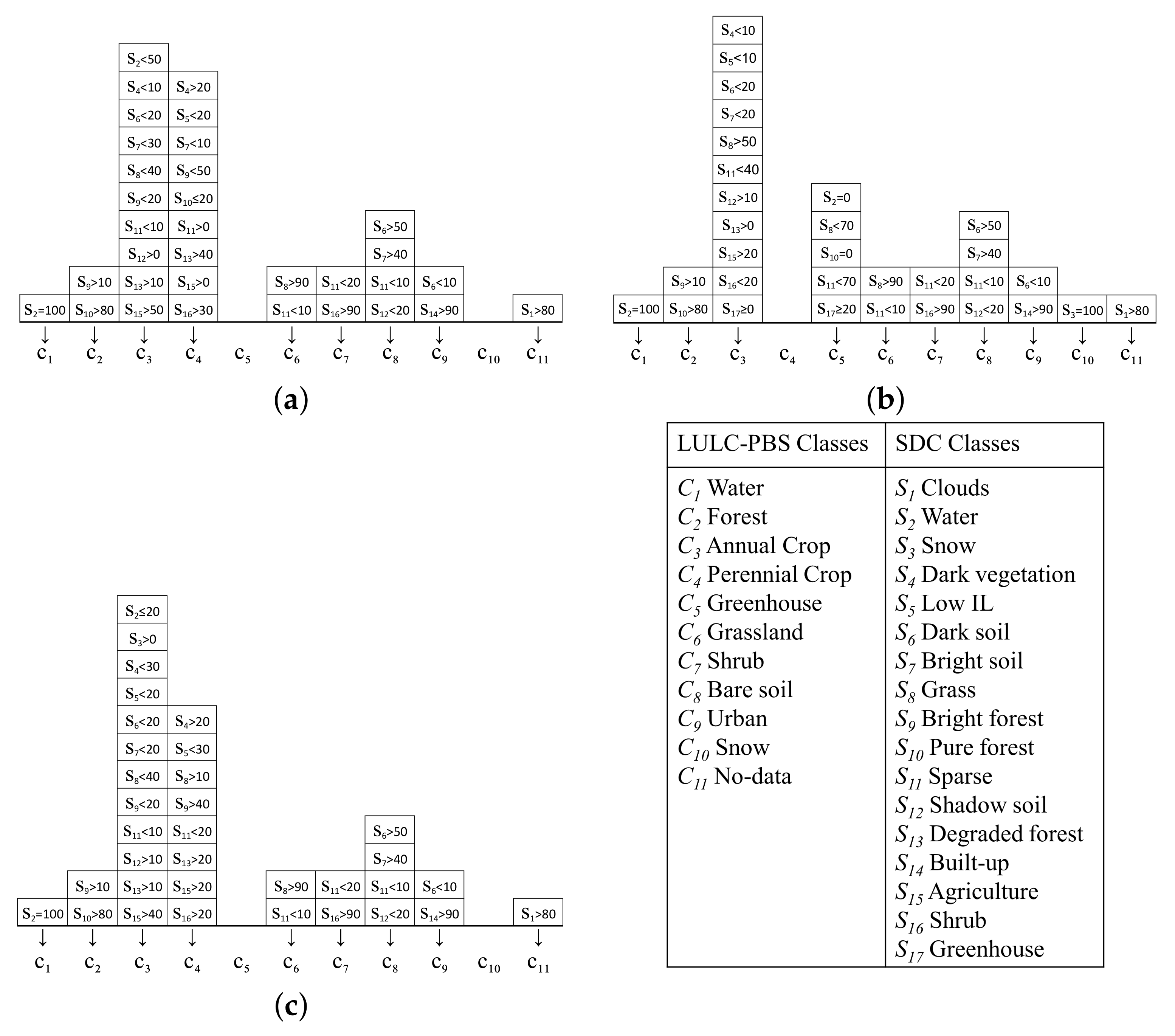
3.1. Rules for New SDC Classes
| Algorithm 1: SDC rules. |
|
Input: UI, BSI, NDBI, NDVI, NDWI, EVI, SAVI, GDVI, EVI, NDTI, VIIRS Output: OutClass Data: Target area dataset  |
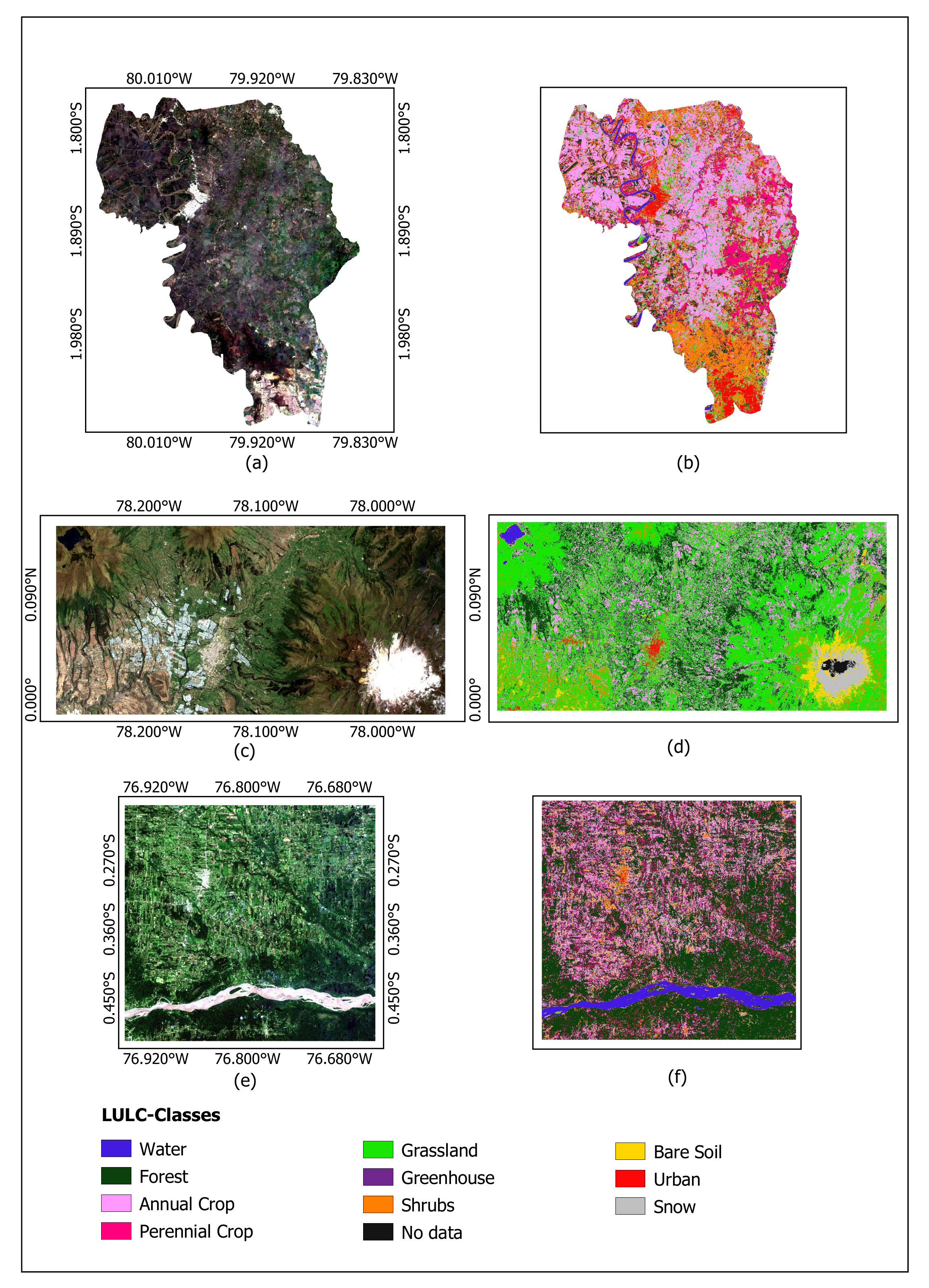
3.2. LULC-PBS Maps
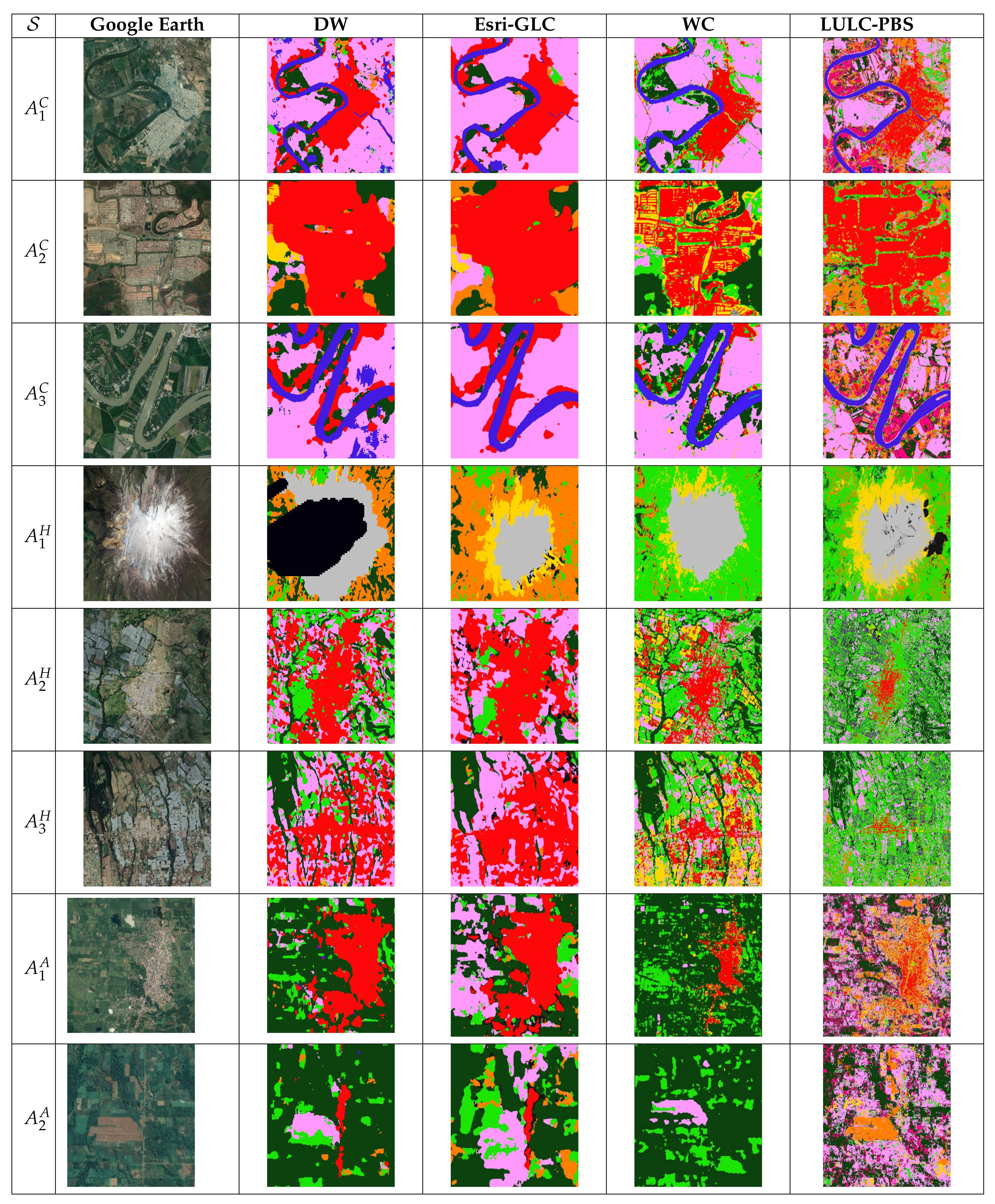
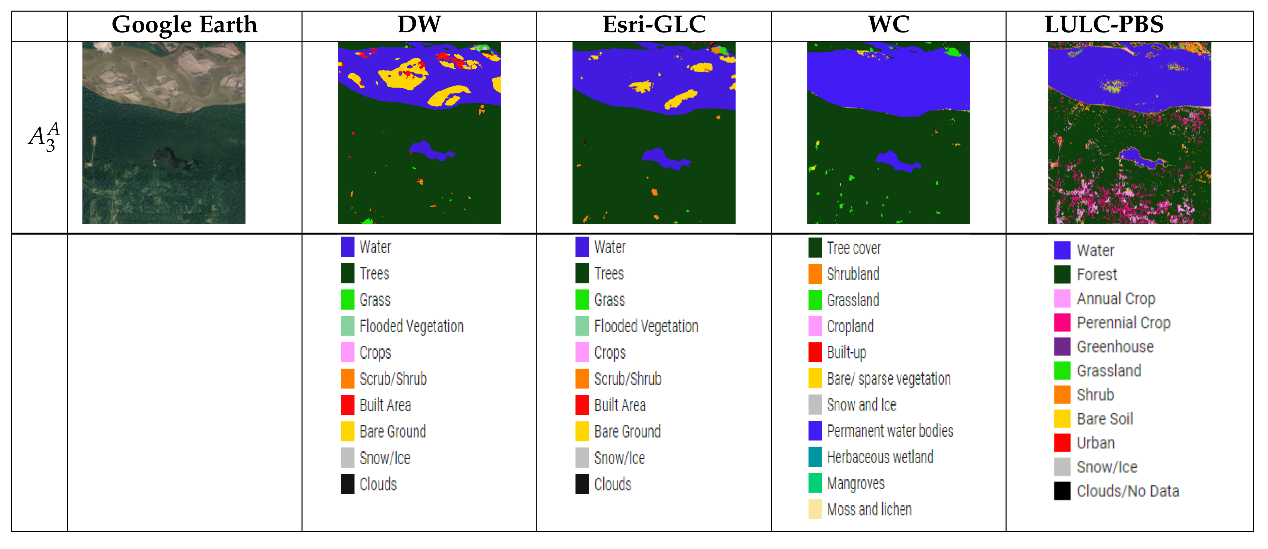
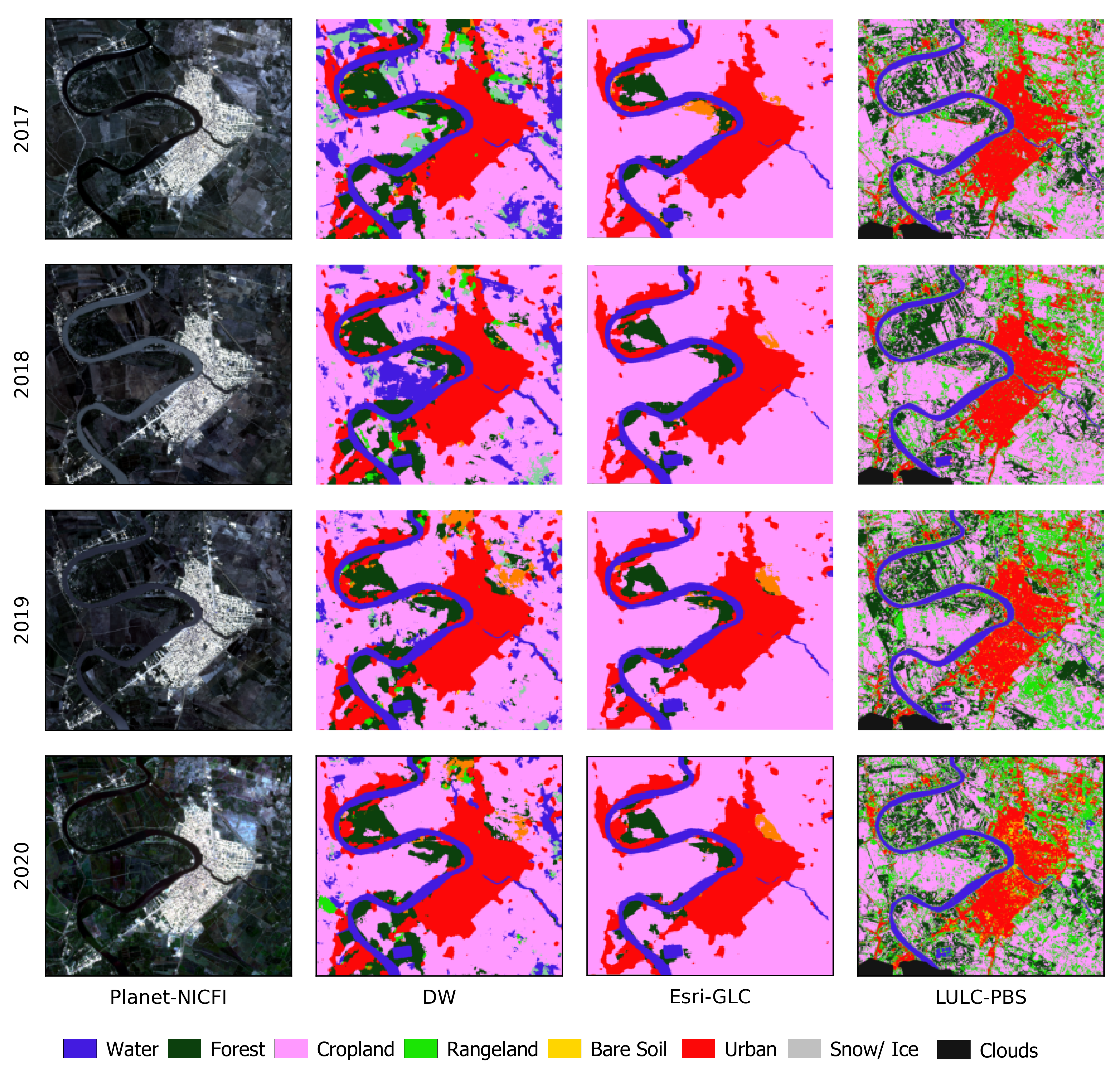
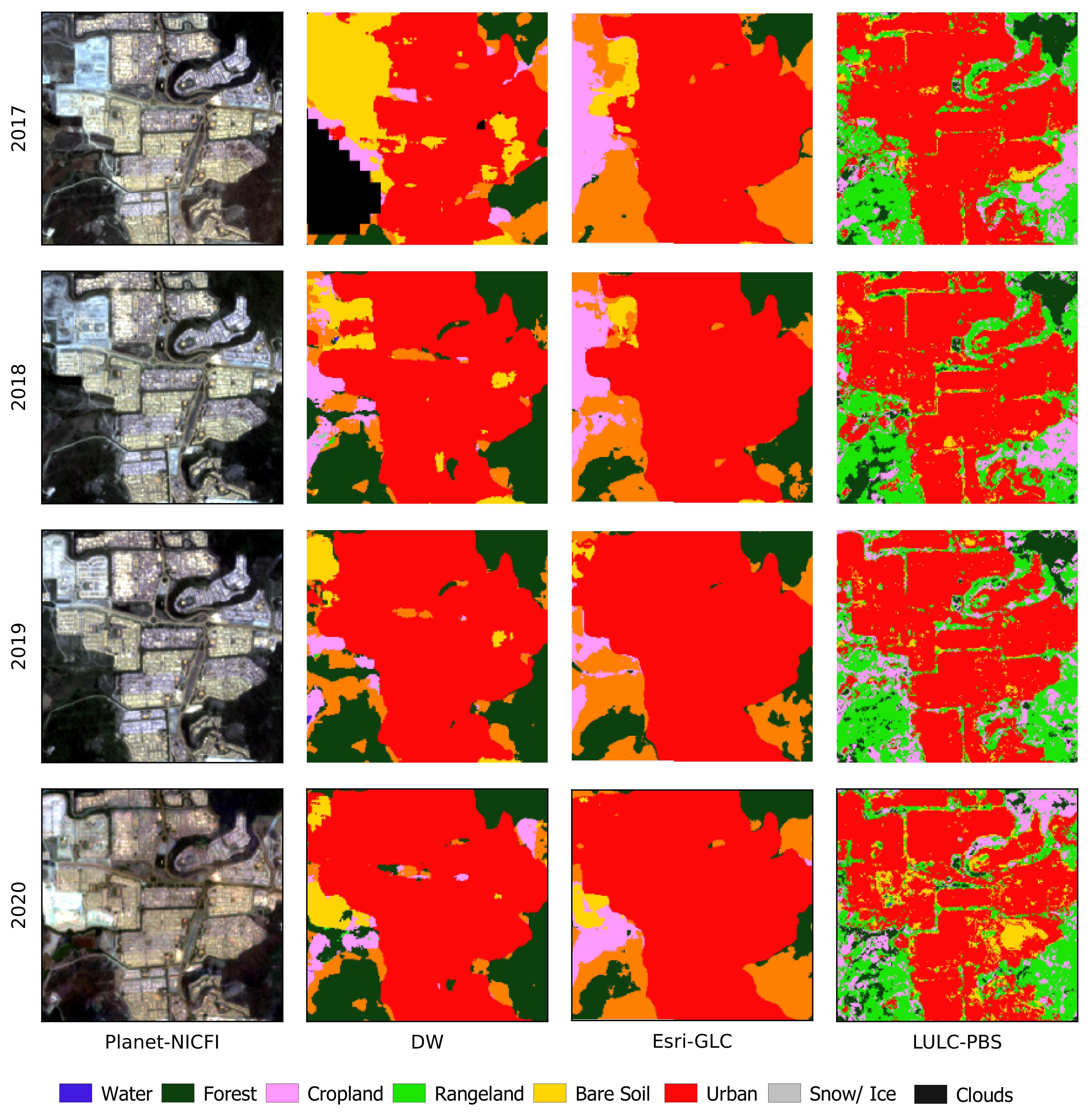
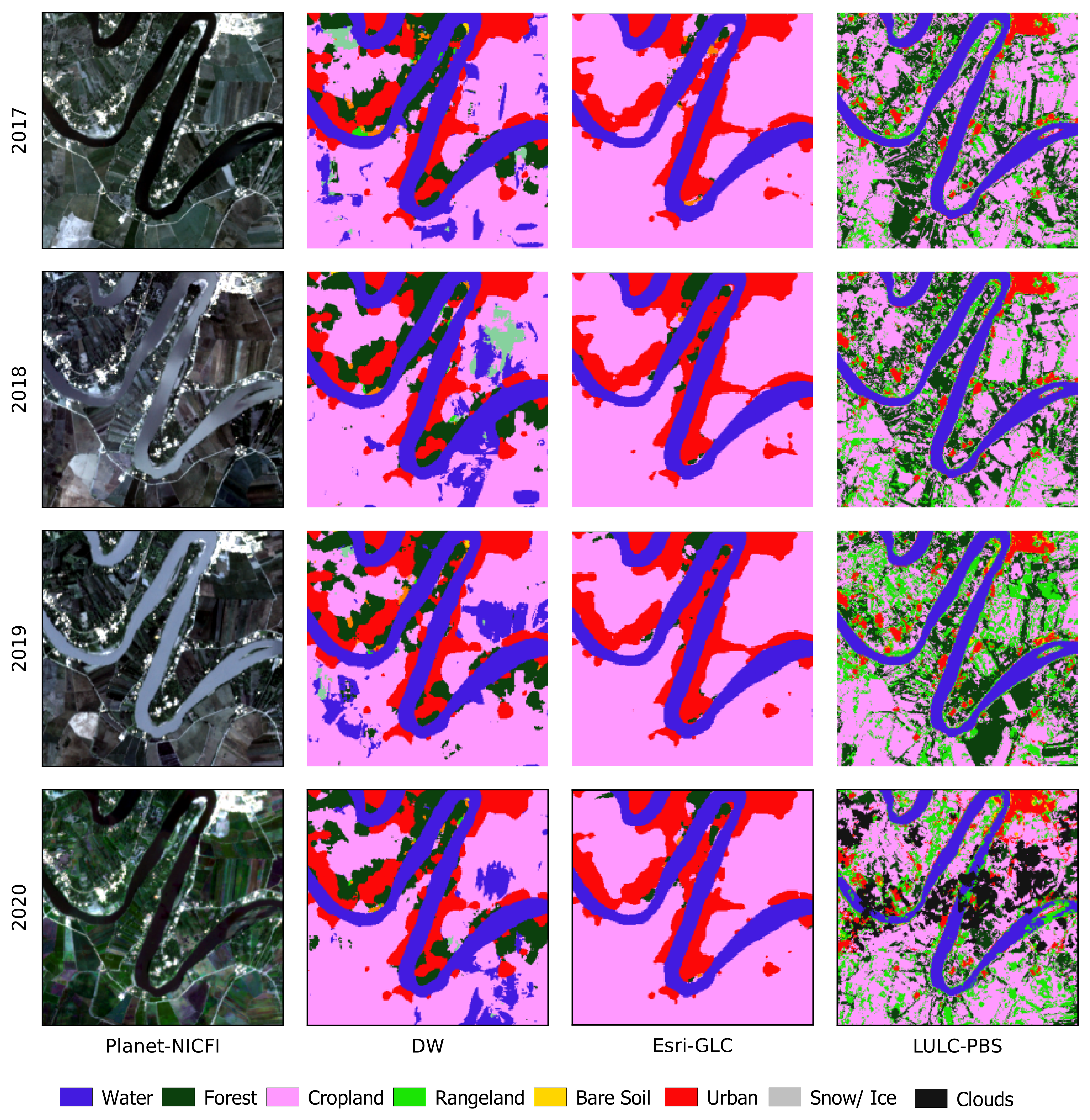
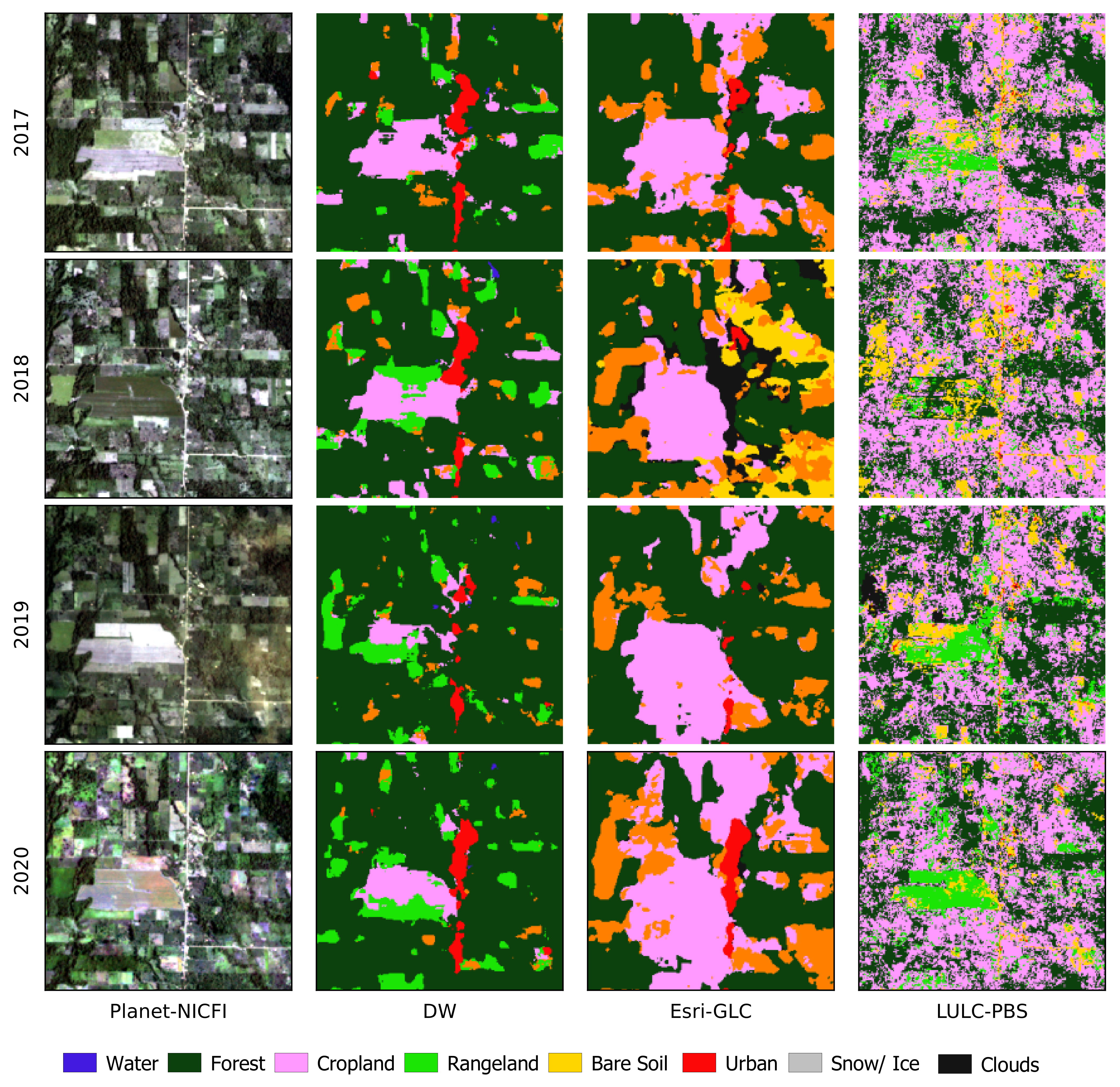
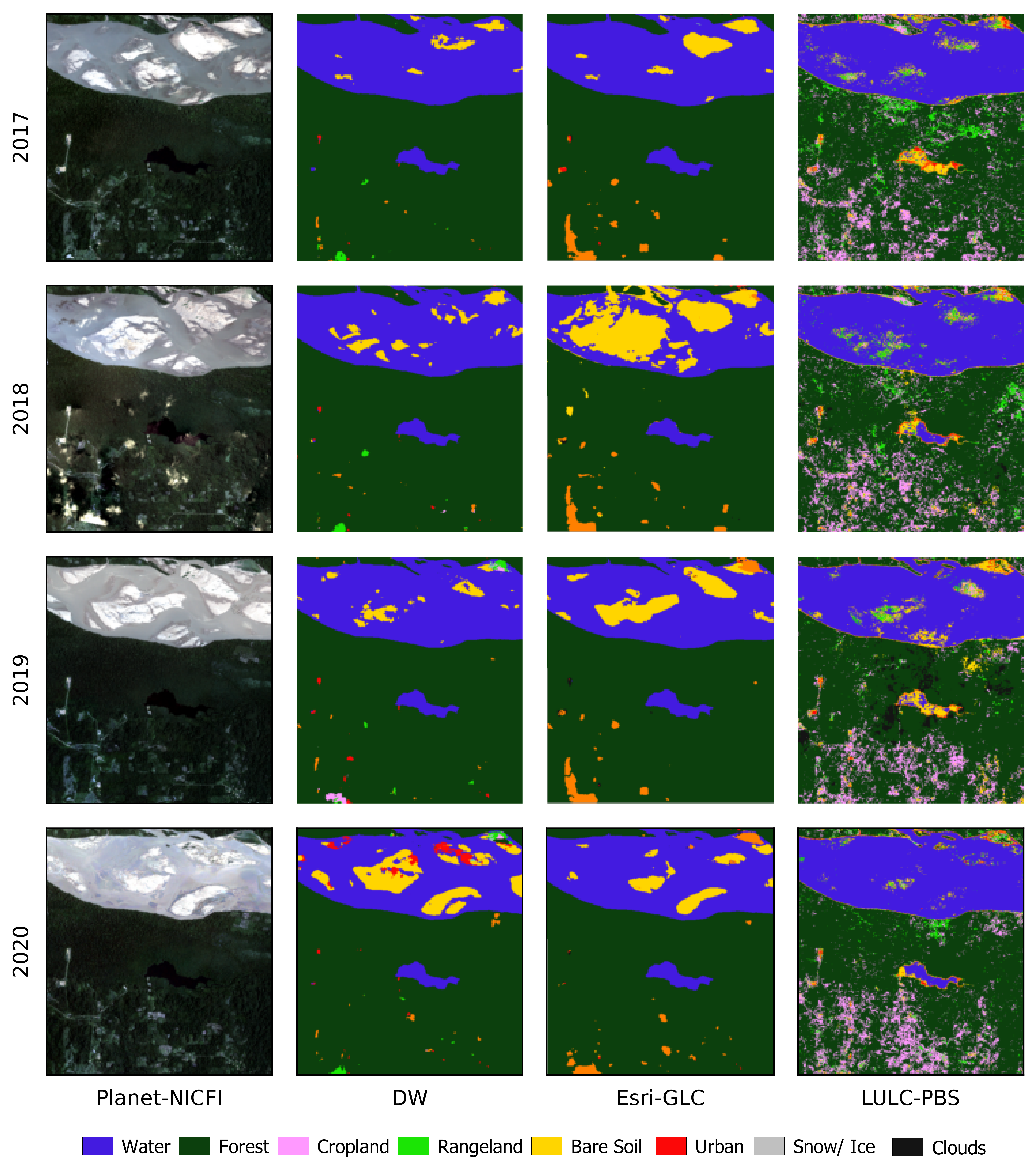
3.3. Visual Comparison of LULC Maps
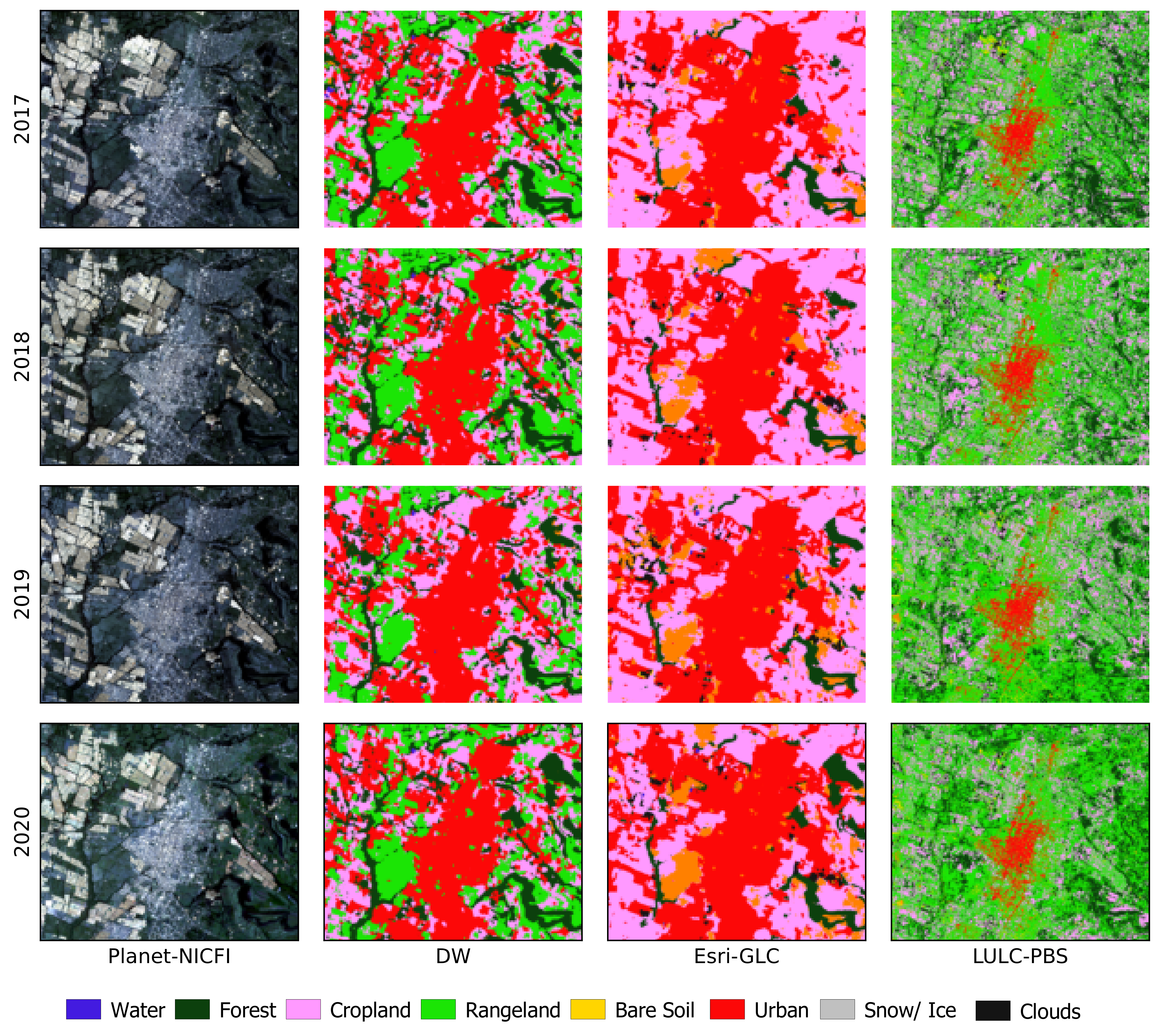
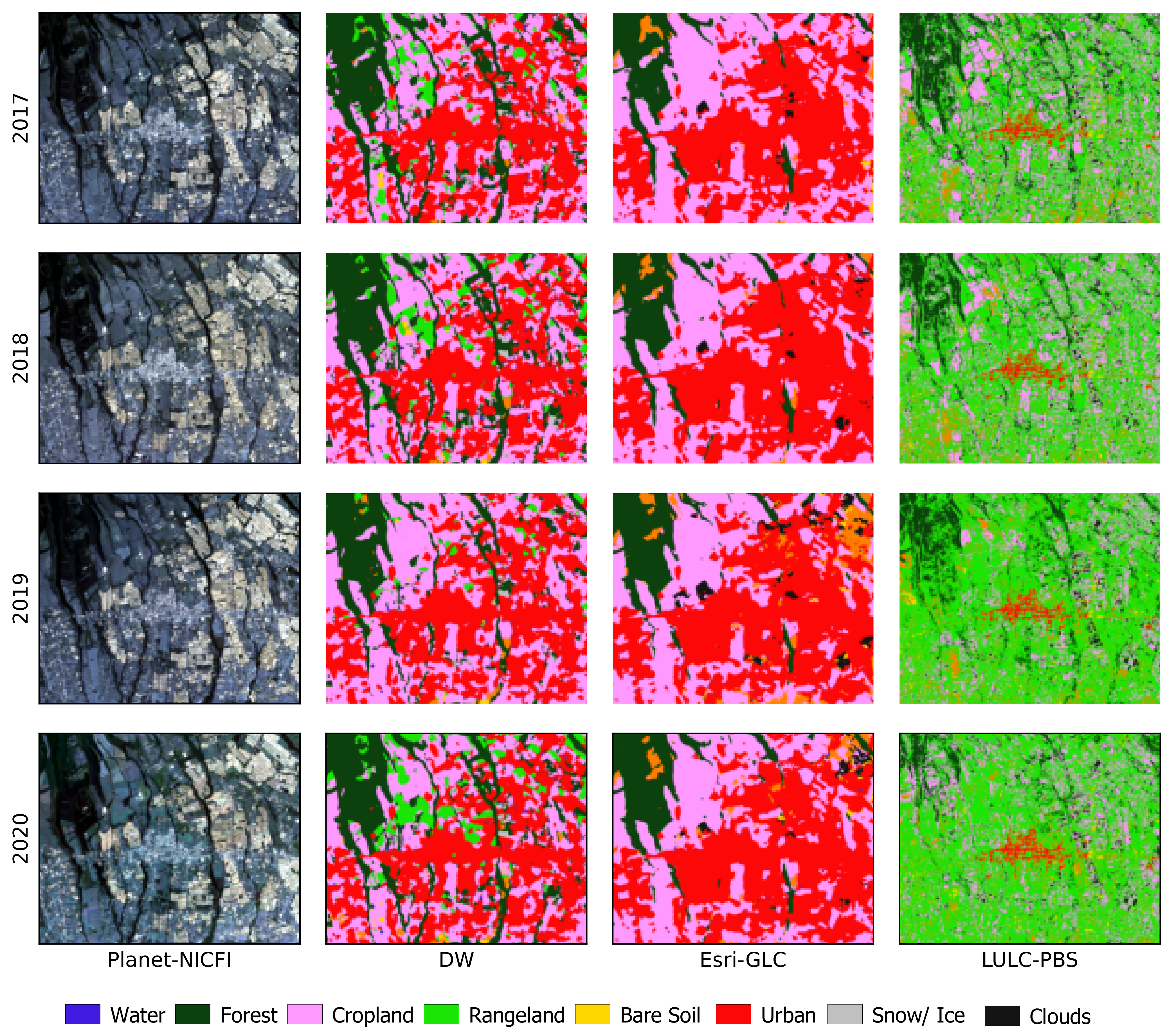
- Dominant Classes: This occurs when pixels of a given class appear more often than the rest in a map. For instance, urban coverage is observed in most pixels of the reference images of sub-areas and with some pixels corresponding to bare ground and vegetation. In WC and LULC-PBS maps, most pixels are classified as urban areas while keeping a proportional relationship to the features seen in the corresponding reference image, whereas Esri-GLC and DW maps show a single large urban patch. Similarly, in sub-area where an urban area is surrounded by vegetation. Here, vegetation could be interpreted as agricultural mosaics, therefore overestimating the predominant land use class. In sub-area , most rivers’ pixels in the reference image were labelled as urban areas in Esri-GLC and DW maps, whereas in the WC map, some of them are detected as bare ground. In the LULC-PBS river, pixels were correctly classified as water.
- Nature-related interclasses conversion: Natural phenomena may cause temporal changes in land cover and consequently ambiguities in pixel-level classification. This effect can be seen in sub-area , in which the reference image shows a river with overbank deposits. These deposits are not detected in WC. LULC-PBS classified them as grassland and both Esri-GLC and DW as bare soil. Similarly, the islet in sub-area only appears in WC and LULC-PBS maps.
- Greenhouses: These structures usually appear in LULC maps as urban or crops pixels as in sub-areas and in DW, Esri-GLC and WC maps and as a greenhouse in the proposed LULC-PBS map.
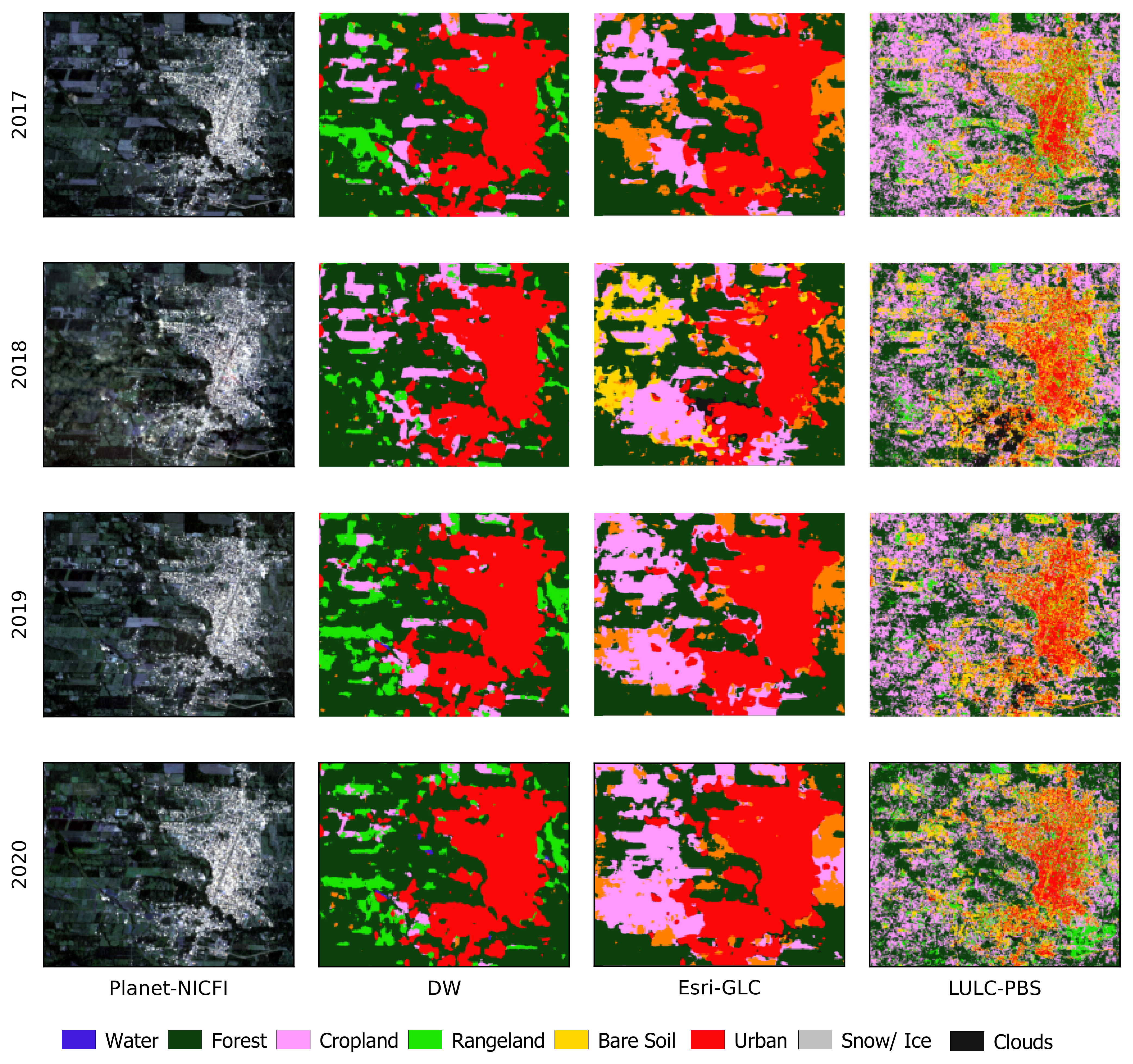
- Phenological stage transitions: For example, in and , a large farmland mosaic in the LULC-PBS map is mapped as grassland in DW and WC products. The Esri-GLC map shows crop areas, although overestimated in size. In the case of sub-area , the reference image contains a large area of the Amazonian forest but also a few crop patches. Global products miss these areas that appear in the LULC-PBS map.
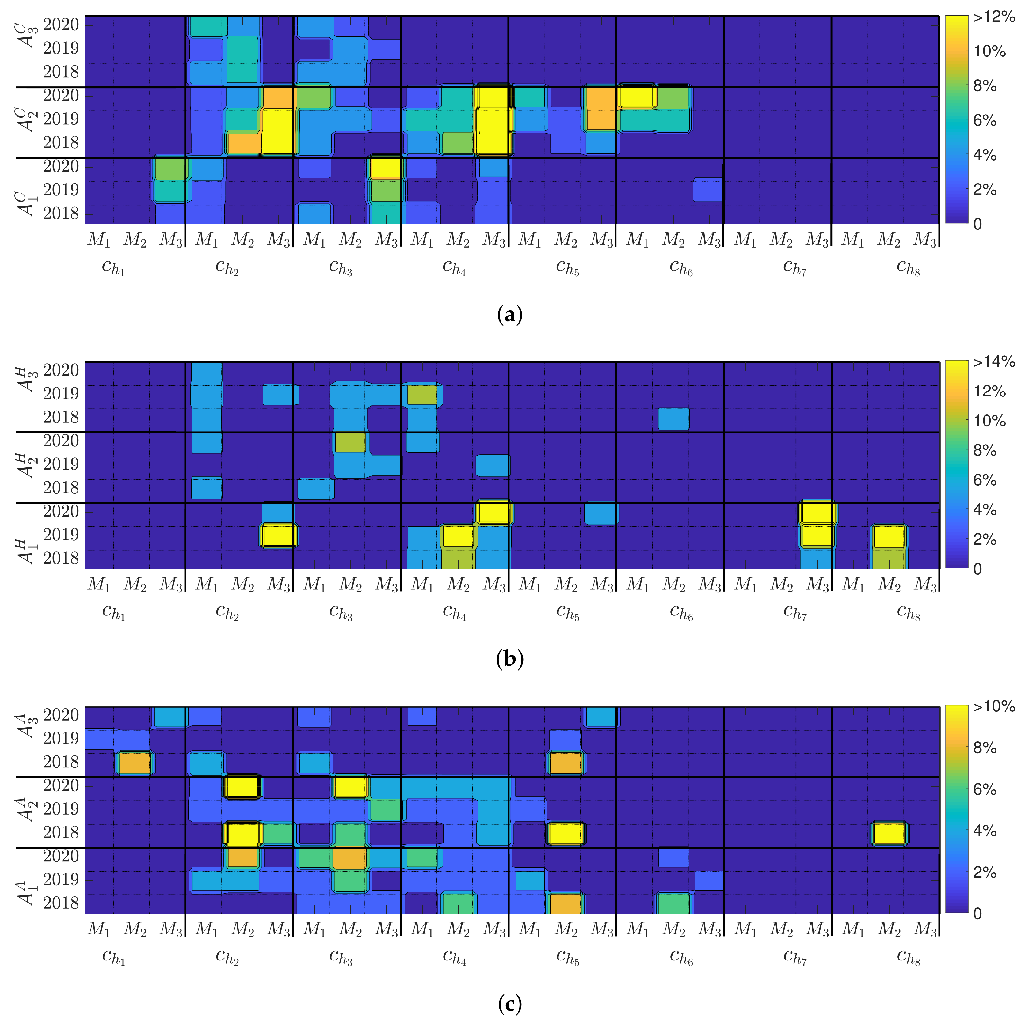
3.4. Surface Area Differences
- Coast sub-areas, see Figure 9a:
- : This area is made up of a rural village, crops, and a large river, and therefore showed slight variations in the vegetation, built-up, and water classes. The LULC-PBS map shows a variation of up to 4% in forest (). LULC-PBS and DW detected changes on surface size from cropland () and rangeland (). Meanwhile, only the DW map showed a variation on water (), between 2% and 6%.
- : Over the years, this area has changed from agricultural cultivation to urban areas, whereby LULC-PBS and Esri-GLC have correctly detected the variations in the surface area of the built () class. Three maps showed variation up to more than 12% in the forest (), rangeland (), and bare soil () classes.
- : Only two types of land cover changed in size, forest area changed between 2% and 7%, and the cropland between 2% and 4% were detected by LULC-PBS and Esri-GLC.
- Andean highland sub-areas, see Figure 9b:
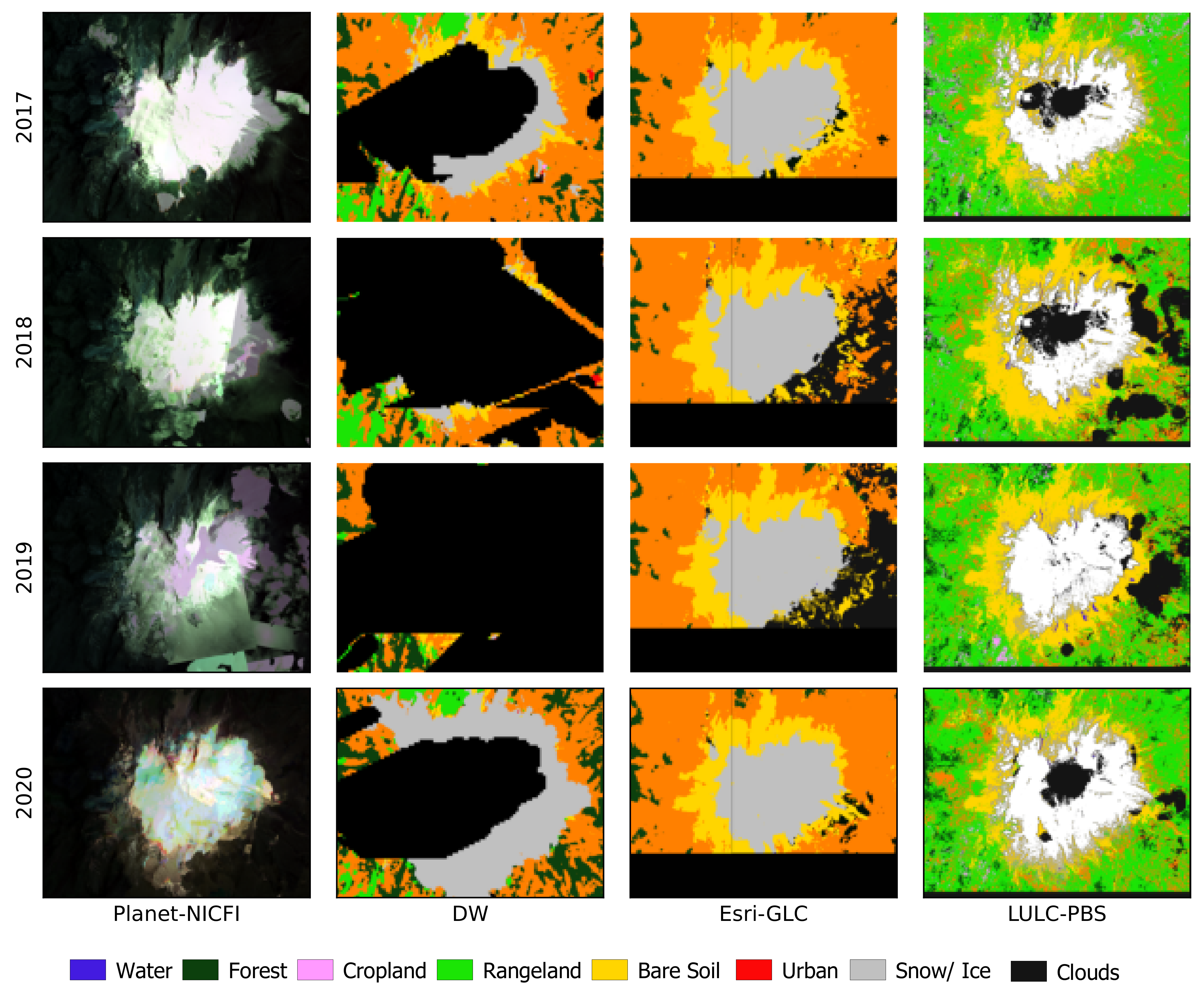
- : This area contains a volcano with its snow cover surrounded by paramo vegetation; thus, all three maps coincided in detecting changes in the rangeland () class. Only the Dynamic world map was able to detect changes up to 14% in the snow () class.
- : LULC-PBS and Esri-GLC detected minor variations, up to 2%, in forest () and rangeland () classes. The cropland class () showed a change in the area up to 14% in all three maps. : forest () and cropland () classes varied in size, by about 6% in LULC-PBS and Esri-GLC, respectively. Rangeland () varied by more than 14% in the PBS-LULC map only.
- Amazon sub-areas, see Figure 9c:
- : It is a small village area surrounded by forest and crops. All three maps detected dynamism among the classes corresponding to vegetation. LULC-PBS was the only map that did not detect any changes in the built () class.
- : It is an area covered with crops. All three maps showed changes of up to 12% in vegetation classes. Meanwhile, the Dynamic world map did not detect any changes in the bare soil () class.
- : This area shows a large forest with patches of cropland. Only LULC-PBS was able to detect variations in the forest () and cropland () classes changed from 2% to 4%. Visual analysis of the study area revealed the presence of a river containing several islets. Our results showed that the Esri-GLC and DW maps indicated changes ranging from 6% to 8% in the bare soil () class, whereas all three maps showed changes in the water () class.
4. Discussion
4.1. PBS Classification
4.2. Global Product Comparison
4.3. Limitations
5. Conclusions and Recommendations
Author Contributions
Funding
Data Availability Statement
Acknowledgments
Conflicts of Interest
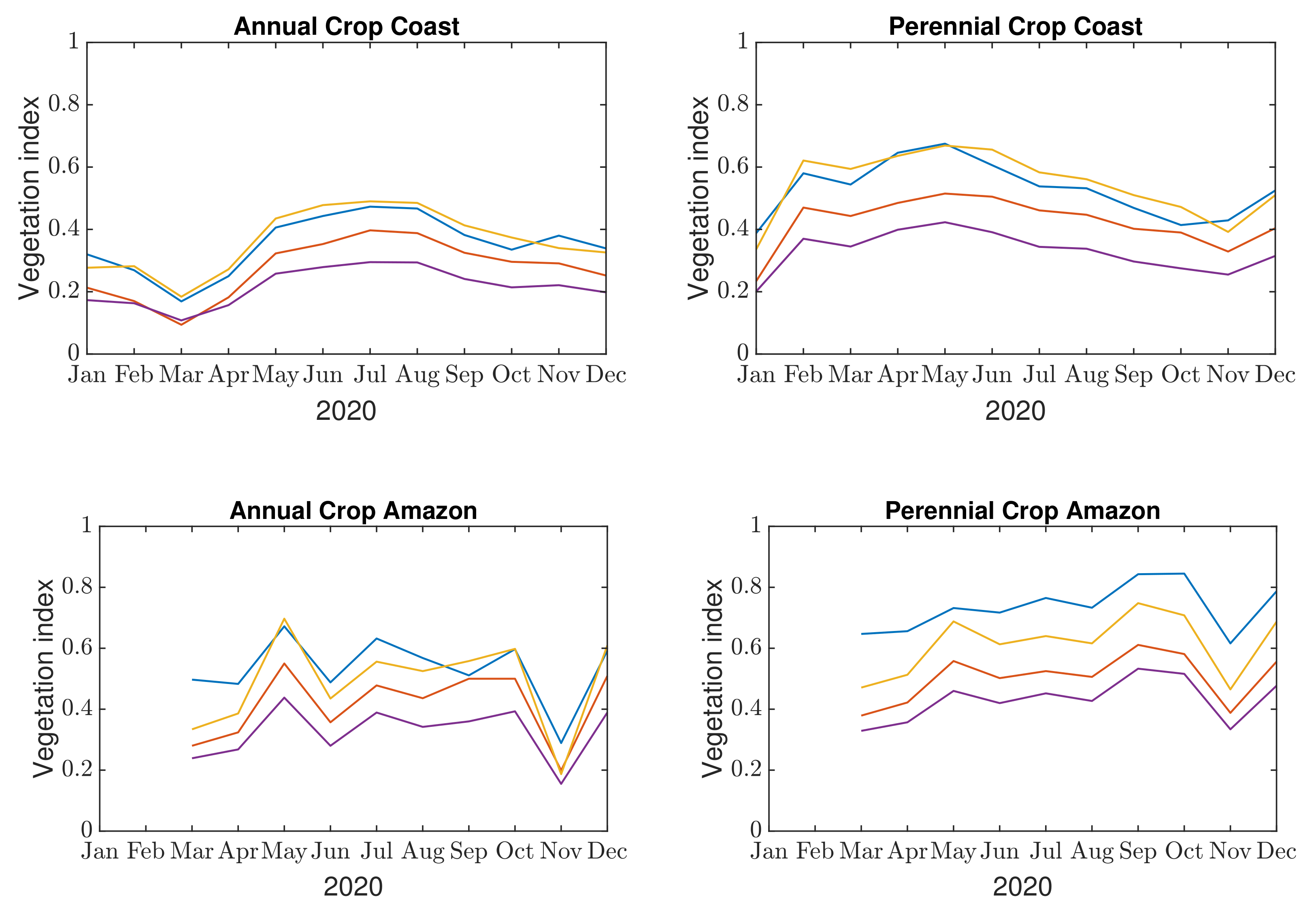
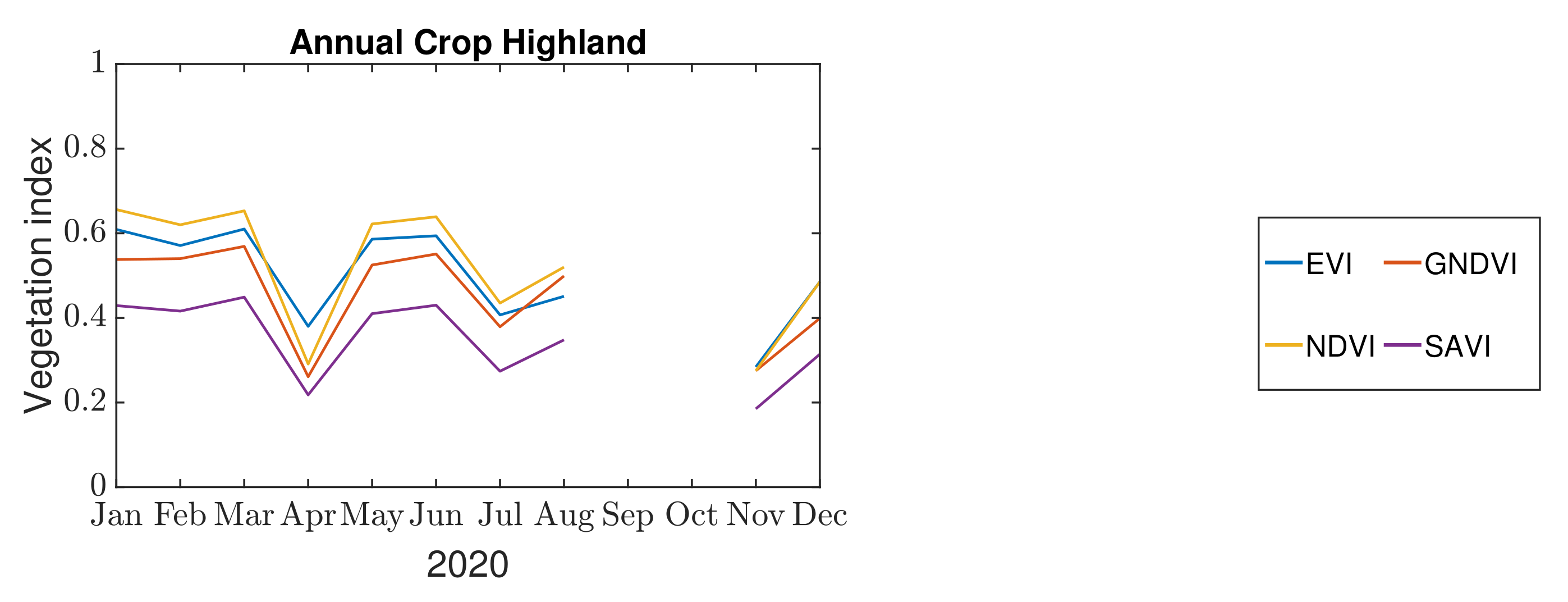
Appendix A. Monthly Spectral Index


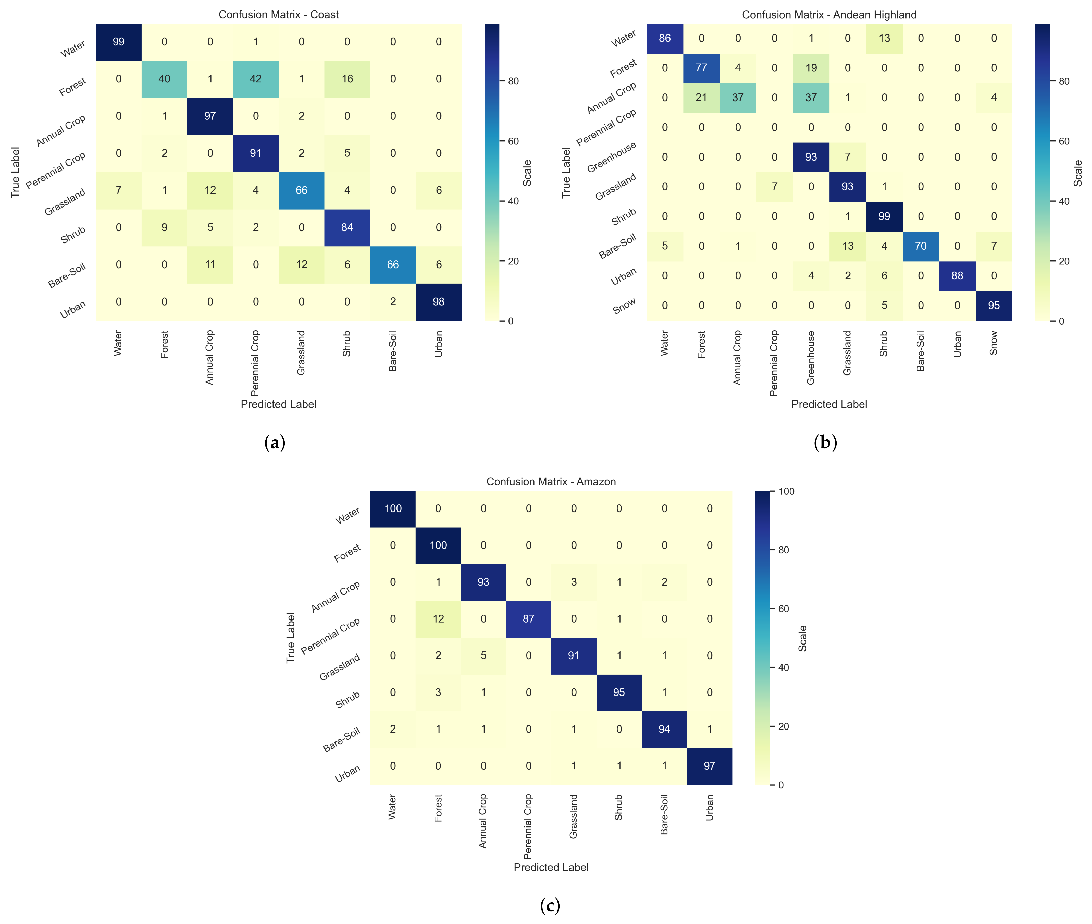
Appendix B. Confusion Matrices

Appendix C. Annual Visual Comparison between Different Land Cover Products in Ecuadorian Ecoregions


References
- Talukdar, S.; Singha, P.; Mahato, S.; Pal, S.; Liou, Y.A.; Rahman, A. Land-use land-cover classification by machine learning classifiers for satellite observations—A review. Remote Sens. 2020, 12, 1135. [Google Scholar] [CrossRef]
- Ngondo, J.; Mango, J.; Liu, R.; Nobert, J.; Dubi, A.; Cheng, H. Land-use and land-cover (LULC) change detection and the implications for coastal water resource management in the Wami–Ruvu Basin, Tanzania. Sustainability 2021, 13, 4092. [Google Scholar] [CrossRef]
- Hansen, M.C.; DeFries, R.S.; Townshend, J.R.; Sohlberg, R. Global land cover classification at 1 km spatial resolution using a classification tree approach. Int. J. Remote Sens. 2000, 21, 1331–1364. [Google Scholar] [CrossRef]
- Loveland, T.R.; Reed, B.C.; Brown, J.F.; Ohlen, D.O.; Zhu, Z.; Yang, L.; Merchant, J.W. Development of a global land cover characteristics database and IGBP DISCover from 1 km AVHRR data. Int. J. Remote Sens. 2000, 21, 1303–1330. [Google Scholar] [CrossRef]
- Friedl, M.A.; Sulla-Menashe, D.; Tan, B.; Schneider, A.; Ramankutty, N.; Sibley, A.; Huang, X. MODIS Collection 5 global land cover: Algorithm refinements and characterization of new datasets. Remote Sens. Environ. 2010, 114, 168–182. [Google Scholar] [CrossRef]
- Bicheron, P.; Leroy, M.; Brockmann, C.; Krämer, U.; Miras, B.; Huc, M.; Ninõ, F.; Defourny, P.; Vancutsem, C.; Arino, O.; et al. GLOBCOVER: A 300 m global land cover product for 2005 using ENVISAT MERIS time series. In Proceedings of the Recent Advances in Quantitative Remote Sensing Symposium, Torrent, Spain, 25–29 September 2006; pp. 538–542. [Google Scholar]
- Karra, K.; Kontgis, C.; Statman-Weil, Z.; Mazzariello, J.C.; Mathis, M.; Brumby, S.P. Global land use/land cover with Sentinel-2 and deep learning. In Proceedings of the IGARSS 2021–2021 IEEE International Geoscience and Remote Sensing Symposium, Brussels, Belgium, 11–16 July 2021. [Google Scholar]
- Zanaga, D.; Van De Kerchove, R.; De Keersmaecker, W.; Souverijns, N.; Brockmann, C.; Quast, R.; Wevers, J.; Grosu, A.; Paccini, A.; Vergnaud, S.; et al. ESA WorldCover 10 m 2020 v100. 2021. Available online: https://developers.google.com/earth-engine/datasets/catalog/ESA_WorldCover_v100#description (accessed on 10 January 2021).
- Brown, C.F.; Brumby, S.P.; Guzder-Williams, B.; Birch, T.; Hyde, S.B.; Mazzariello, J.; Czerwinski, W.; Pasquarella, V.J.; Haertel, R.; Ilyushchenko, S.; et al. Dynamic World, Near real-time global 10 m land use land cover mapping. Sci. Data 2022, 9, 251. [Google Scholar] [CrossRef]
- Chaaban, F.; El Khattabi, J.; Darwishe, H. Accuracy Assessment of ESA WorldCover 2020 and ESRI 2020 Land Cover Maps for a Region in Syria. J. Geovis. Spat. Anal. 2022, 6, 31. [Google Scholar] [CrossRef]
- Wang, J.; Yang, X.; Wang, Z.; Cheng, H.; Kang, J.; Tang, H.; Li, Y.; Bian, Z.; Bai, Z. Consistency Analysis and Accuracy Assessment of Three Global Ten-Meter Land Cover Products in Rocky Desertification Region—A Case Study of Southwest China. Isprs Int. J. Geo-Inf. 2022, 11, 202. [Google Scholar] [CrossRef]
- Pandey, P.C.; Koutsias, N.; Petropoulos, G.P.; Srivastava, P.K.; Ben Dor, E. Land use/land cover in view of earth observation: Data sources, input dimensions, and classifiers—A review of the state of the art. Geocarto Int. 2021, 36, 957–988. [Google Scholar] [CrossRef]
- Alshari, E.A.; Gawali, B.W. Development of classification system for LULC using remote sensing and GIS. Glob. Transitions Proc. 2021, 2, 8–17. [Google Scholar] [CrossRef]
- Omeer, A.A.; Deshmukh, R.R.; Gupta, R.S.; Kayte, J.N. Land Use and Cover Mapping Using SVM and MLC Classifiers: A Case Study of Aurangabad City, Maharashtra, India. In Proceedings of the International Conference on Recent Trends in Image Processing and Pattern Recognition, Solapur, India, 21–22 December 2018; Springer: Berlin/Heidelberg, Germany, 2018; pp. 482–492. [Google Scholar] [CrossRef]
- Loukika, K.N.; Keesara, V.R.; Sridhar, V. Analysis of Land Use and Land Cover Using Machine Learning Algorithms on Google Earth Engine for Munneru River Basin, India. Sustainability 2021, 13, 13758. [Google Scholar] [CrossRef]
- Varade, D.; Sure, A.; Dikshit, O. Potential of Landsat-8 and Sentinel-2A composite for land use land cover analysis. Geocarto Int. 2019, 34, 1552–1567. [Google Scholar] [CrossRef]
- Khan, A.; Govil, H.; Kumar, G.; Dave, R. Synergistic use of Sentinel-1 and Sentinel-2 for improved LULC mapping with special reference to bad land class: A case study for Yamuna River floodplain, India. Spat. Inf. Res. 2020, 28, 669–681. [Google Scholar] [CrossRef]
- Sánchez-Espinosa, A.; Schröder, C. Land use and land cover mapping in wetlands one step closer to the ground: Sentinel-2 versus landsat 8. J. Environ. Manag. 2019, 247, 484–498. [Google Scholar] [CrossRef]
- Yan, E.; Wang, G.; Lin, H.; Xia, C.; Sun, H. Phenology-based classification of vegetation cover types in Northeast China using MODIS NDVI and EVI time series. Int. J. Remote Sens. 2015, 36, 489–512. [Google Scholar] [CrossRef]
- Htitiou, A.; Boudhar, A.; Lebrini, Y.; Hadria, R.; Lionboui, H.; Elmansouri, L.; Tychon, B.; Benabdelouahab, T. The performance of random forest classification based on phenological metrics derived from Sentinel-2 and Landsat 8 to map crop cover in an irrigated semi-arid region. Remote Sens. Earth Syst. Sci. 2019, 2, 208–224. [Google Scholar] [CrossRef]
- Kpienbaareh, D.; Sun, X.; Wang, J.; Luginaah, I.; Bezner Kerr, R.; Lupafya, E.; Dakishoni, L. Crop type and land cover mapping in northern Malawi using the integration of sentinel-1, sentinel-2, and planetscope satellite data. Remote Sens. 2021, 13, 700. [Google Scholar] [CrossRef]
- Solórzano, J.V.; Mas, J.F.; Gao, Y.; Gallardo-Cruz, J.A. Land use land cover classification with U-net: Advantages of combining sentinel-1 and sentinel-2 imagery. Remote Sens. 2021, 13, 3600. [Google Scholar] [CrossRef]
- Zhang, X.y.; Feng, X.z.; Deng, H. Land-cover density-based approach to urban land use mapping using high-resolution imagery. Chin. Geogr. Sci. 2005, 15, 162–167. [Google Scholar] [CrossRef]
- Zhang, Y.; Li, Q.; Huang, H.; Wu, W.; Du, X.; Wang, H. The combined use of remote sensing and social sensing data in fine-grained urban land use mapping: A case study in Beijing, China. Remote Sens. 2017, 9, 865. [Google Scholar] [CrossRef]
- Johnson, B.A.; Iizuka, K. Integrating OpenStreetMap crowdsourced data and Landsat time-series imagery for rapid land use/land cover (LULC) mapping: Case study of the Laguna de Bay area of the Philippines. Appl. Geogr. 2016, 67, 140–149. [Google Scholar] [CrossRef]
- Huan, V. Accuracy assessment of land use land cover LULC 2020 (ESRI) data in Con Dao island, Ba Ria–Vung Tau province, Vietnam. In Proceedings of the IOP Conference Series: Earth and Environmental Science, Online, 28–29 December 2022; IOP Publishing: Bristol, UK, 2022; Volume 1028, p. 012010. [Google Scholar]
- Liu, X.; He, J.; Yao, Y.; Zhang, J.; Liang, H.; Wang, H.; Hong, Y. Classifying urban land use by integrating remote sensing and social media data. Int. J. Geogr. Inf. Sci. 2017, 31, 1675–1696. [Google Scholar] [CrossRef]
- Jia, Y.; Ge, Y.; Ling, F.; Guo, X.; Wang, J.; Wang, L.; Chen, Y.; Li, X. Urban land use mapping by combining remote sensing imagery and mobile phone positioning data. Remote Sens. 2018, 10, 446. [Google Scholar] [CrossRef]
- Yonaba, R.; Koïta, M.; Mounirou, L.; Tazen, F.; Queloz, P.; Biaou, A.; Niang, D.; Zouré, C.; Karambiri, H.; Yacouba, H. Spatial and transient modelling of land use/land cover (LULC) dynamics in a Sahelian landscape under semi-arid climate in northern Burkina Faso. Land Use Policy 2021, 103, 105305. [Google Scholar] [CrossRef]
- Zhao, Y.; Feng, D.; Yu, L.; Wang, X.; Chen, Y.; Bai, Y.; Hernández, H.J.; Galleguillos, M.; Estades, C.; Biging, G.S.; et al. Detailed dynamic land cover mapping of Chile: Accuracy improvement by integrating multi-temporal data. Remote Sens. Environ. 2016, 183, 170–185. [Google Scholar] [CrossRef]
- Mapa de Precipitación Media Multianual. 1965–1999. Available online: https://www.inamhi.gob.ec/docum_institucion/MapasBiblioteca/5%20PrecipitacionA0.pdf (accessed on 5 March 2020).
- Plan de Desarrollo y Ordenamiento Territorial del Cantón Daule 2015–2025. 2015. Available online: https://www.daule.gob.ec/documents/20124/39854/PDOT_DAULE_2015-2025.pdf (accessed on 10 January 2021).
- Hribljan, J.A.; Suárez, E.; Heckman, K.A.; Lilleskov, E.A.; Chimner, R.A. Peatland carbon stocks and accumulation rates in the Ecuadorian páramo. Wetl. Ecol. Manag. 2016, 24, 113–127. [Google Scholar] [CrossRef]
- Pitman, N.C.A. A Large-Scale Inventory of Two Amazonian Tree Communities; Duke University: Durham, NC, USA, 2000. [Google Scholar]
- Plan de Desarrollo y Ordenamiento Territorial de la Provincia de Orellana 2015–2019. 2015. Available online: https://www.gporellana.gob.ec/wp-content/uploads/2015/11/PDYOT-2015-2019_ORELLANA_ACTUALIZADO.pdf (accessed on 10 January 2021).
- Small, C. Multisensor characterization of urban morphology and network structure. Remote Sens. 2019, 11, 2162. [Google Scholar] [CrossRef]
- Liu, Z.; Zhang, Q.; Yue, D.; Hao, Y.; Su, K. Extraction of urban built-up areas based on Sentinel-2A and NPP-VIIRS nighttime light data. Remote Sens. Land Resour. 2019, 4, 227–234. [Google Scholar]
- Song, Y.; Chen, B.; Kwan, M.P. How does urban expansion impact people’s exposure to green environments? A comparative study of 290 Chinese cities. J. Clean. Prod. 2020, 246, 119018. [Google Scholar] [CrossRef]
- Asner, G.P. Cloud cover in Landsat observations of the Brazilian Amazon. Int. J. Remote Sens. 2001, 22, 3855–3862. [Google Scholar] [CrossRef]
- Mills, S.; Weiss, S.; Liang, C. VIIRS day/night band (DNB) stray light characterization and correction. In Proceedings of the Earth Observing Systems XVIII, International Society for Optics and Photonics, Bellingham, WA, USA, 22–24 August 2013; Volume 8866, p. 88661. [Google Scholar]
- Simonetti, D.; Simonetti, E.; Szantoi, Z.; Lupi, A.; Eva, H. First results from the phenology-based synthesis classifier using Landsat 8 imagery. IEEE Geosci. Remote Sens. Lett. 2015, 12, 1496–1500. [Google Scholar] [CrossRef]
- Zhao, Y.; Gong, P.; Yu, L.; Hu, L.; Li, X.; Li, C.; Zhang, H.; Zheng, Y.; Wang, J.; Zhao, Y.; et al. Towards a common validation sample set for global land-cover mapping. Int. J. Remote Sens. 2014, 35, 4795–4814. [Google Scholar] [CrossRef]
- Arief, M.C.W.; Itaya, A. A Brief Description of Recovery Process of Coastal Vegetation after Tsunami: A Google Earth Time-Series Remote Sensing Data. J. Manaj. Hutan Trop. 2017, 23, 81–89. [Google Scholar] [CrossRef]
- Simonetti, E.; Simonetti, D.; Preatoni, D. Phenology-Based Land Cover Classification Using Landsat 8 Time Series; European Commission Joint Research Center: Ispra, Italy, 2014. [Google Scholar]
- Nguyen, T.T.H.; De Bie, C.; Ali, A.; Smaling, E.; Chu, T.H. Mapping the irrigated rice cropping patterns of the Mekong delta, Vietnam, through hyper-temporal SPOT NDVI image analysis. Int. J. Remote Sens. 2012, 33, 415–434. [Google Scholar] [CrossRef]
- Huang, H.; Roy, D.P.; Boschetti, L.; Zhang, H.K.; Yan, L.; Kumar, S.S.; Gomez-Dans, J.; Li, J. Separability analysis of Sentinel-2A multi-spectral instrument (MSI) data for burned area discrimination. Remote Sens. 2016, 8, 873. [Google Scholar] [CrossRef]
- Chen, Y.; Zhang, L.; Li, J.; Shi, Y. Domain driven two-phase feature selection method based on Bhattacharyya distance and kernel distance measurements. In Proceedings of the 2011 IEEE/WIC/ACM International Conferences on Web Intelligence and Intelligent Agent Technology, Lyon, France, 22–27 August 2011; Volume 3, pp. 217–220. [Google Scholar]
- Wang, J.; Feng, Z.; Lu, N.; Luo, J. Toward optimal feature and time segment selection by divergence method for EEG signals classification. Comput. Biol. Med. 2018, 97, 161–170. [Google Scholar] [CrossRef]
- Dabboor, M.; Howell, S.; Shokr, M.; Yackel, J. The Jeffries–Matusita distance for the case of complex Wishart distribution as a separability criterion for fully polarimetric SAR data. Int. J. Remote Sens. 2014, 35, 6859–6873. [Google Scholar]
- Tucker, C.J.; Slayback, D.A.; Pinzon, J.E.; Los, S.O.; Myneni, R.B.; Taylor, M.G. Higher northern latitude normalized difference vegetation index and growing season trends from 1982 to 1999. Int. J. Biometeorol. 2001, 45, 184–190. [Google Scholar] [CrossRef]
- Roy, P.; Miyatake, S.; Rikimaru, A. Biophysical spectral response modeling approach for forest density stratification. In Proceedings of the 18th Asian Conference on Remote Sensing, Kuala Lumpur, Malaysia, 20–24 October 1997. [Google Scholar]
- Kawamura, M.; Jayamanna, S.; Tsujiko, Y. Quantitative evaluation of urbanization in developing countries using satellite data. Doboku Gakkai Ronbunshu 1997, 1997, 45–54. [Google Scholar] [CrossRef]
- Zha, Y.; Gao, J.; Ni, S. Use of normalized difference built-up index in automatically mapping urban areas from TM imagery. Int. J. Remote Sens. 2003, 24, 583–594. [Google Scholar] [CrossRef]
- Ettehadi Osgouei, P.; Kaya, S.; Sertel, E.; Alganci, U. Separating built-up areas from bare land in mediterranean cities using sentinel-2a imagery. Remote Sens. 2019, 11, 345. [Google Scholar] [CrossRef]
- Yang, X.; Zhao, S.; Qin, X.; Zhao, N.; Liang, L. Mapping of urban surface water bodies from Sentinel-2 MSI imagery at 10 m resolution via NDWI-based image sharpening. Remote Sens. 2017, 9, 596. [Google Scholar] [CrossRef]
- Gascoin, S.; Barrou Dumont, Z.; Deschamps-Berger, C.; Marti, F.; Salgues, G.; López-Moreno, J.I.; Revuelto, J.; Michon, T.; Schattan, P.; Hagolle, O. Estimating fractional snow cover in open terrain from sentinel-2 using the normalized difference snow index. Remote Sens. 2020, 12, 2904. [Google Scholar] [CrossRef]
- Gitelson, A.A.; Kaufman, Y.J.; Merzlyak, M.N. Use of a green channel in remote sensing of global vegetation from EOS-MODIS. Remote Sens. Environ. 1996, 58, 289–298. [Google Scholar] [CrossRef]
- Rondeaux, G.; Steven, M.; Baret, F. Optimization of soil-adjusted vegetation indices. Remote Sens. Environ. 1996, 55, 95–107. [Google Scholar] [CrossRef]
- Huete, A.; Didan, K.; Miura, T.; Rodriguez, E.P.; Gao, X.; Ferreira, L.G. Overview of the radiometric and biophysical performance of the MODIS vegetation indices. Remote Sens. Environ. 2002, 83, 195–213. [Google Scholar] [CrossRef]
- Lillesand, T.; Kiefer, R.W.; Chipman, J. Remote Sensing and Image Interpretation; John Wiley & Sons: Hoboken, NJ, USA, 2015. [Google Scholar]
- Li, X.; Zhao, L.; Li, D.; Xu, H. Mapping urban extent using Luojia 1–01 nighttime light imagery. Sensors 2018, 18, 3665. [Google Scholar] [CrossRef]
- Zimmermann, P.; Tasser, E.; Leitinger, G.; Tappeiner, U. Effects of land-use and land-cover pattern on landscape-scale biodiversity in the European Alps. Agric. Ecosyst. Environ. 2010, 139, 13–22. [Google Scholar] [CrossRef]
- Murad, C.A.; Pearse, J. Landsat study of deforestation in the Amazon region of Colombia: Departments of Caquetá and Putumayo. Remote Sens. Appl. Soc. Environ. 2018, 11, 161–171. [Google Scholar] [CrossRef]
- Farjad, B.; Gupta, A.; Razavi, S.; Faramarzi, M.; Marceau, D.J. An integrated modelling system to predict hydrological processes under climate and land-use/cover change scenarios. Water 2017, 9, 767. [Google Scholar] [CrossRef]
- Samal, D.R.; Gedam, S.S. Monitoring land use changes associated with urbanization: An object based image analysis approach. Eur. J. Remote Sens. 2015, 48, 85–99. [Google Scholar] [CrossRef]
- Wang, R.; Kalin, L.; Kuang, W.; Tian, H. Individual and combined effects of land use/cover and climate change on Wolf Bay watershed streamflow in southern Alabama. Hydrol. Process. 2014, 28, 5530–5546. [Google Scholar] [CrossRef]
- Kang, J.; Yang, X.; Wang, Z.; Cheng, H.; Wang, J.; Tang, H.; Li, Y.; Bian, Z.; Bai, Z. Comparison of Three Ten Meter Land Cover Products in a Drought Region: A Case Study in Northwestern China. Land 2022, 11, 427. [Google Scholar] [CrossRef]
- Venter, Z.S.; Barton, D.N.; Chakraborty, T.; Simensen, T.; Singh, G. Global 10 m Land Use Land Cover Datasets: A Comparison of Dynamic World, World Cover and Esri Land Cover. Remote Sens. 2022, 14, 4101. [Google Scholar] [CrossRef]
- Alava Portugal, C.; Hechavarría Hernández, J.R.; Fois Lugo, M. Systemic approach to the territorial planning of the urban Parish La Aurora, Daule, Ecuador. In Proceedings of the International Conference on Intelligent Human Systems Integration, Modena, Italy, 19–21 February 2020; Springer: Berlin/Heidelberg, Germany, 2020; pp. 1201–1205. [Google Scholar]
- Zambrano Murillo, C.; Hechavarría Hernández, J.R.; Leyva Vázquez, M. Environmental Certification Proposal for Sustainable Buildings in the Satellite Parish “La Aurora”, Guayas, Ecuador. In Proceedings of the International Conference on Applied Human Factors and Ergonomics, San Diego, CA, USA, 16–20 July 2020; Springer: Berlin/Heidelberg, Germany, 2020; pp. 63–70. [Google Scholar]
- López, S. Deforestation, forest degradation, and land use dynamics in the Northeastern Ecuadorian Amazon. Appl. Geogr. 2022, 145, 102749. [Google Scholar] [CrossRef]
- Santos, F.; Meneses, P.; Hostert, P. Monitoring long-term forest dynamics with scarce data: A multi-date classification implementation in the Ecuadorian Amazon. Eur. J. Remote Sens. 2019, 52, 62–78. [Google Scholar] [CrossRef]
- Moulatlet, G.M.; Ambriz, E.; Guevara, J.; Lopez, K.G.; Rodes-Blanco, M.; Guerra-Arevalo, N.; Ortega-Andrade, H.M.; Meneses, P. Multi-taxa ecological responses to habitat loss and fragmentation in western Amazonia as revealed by RAPELD biodiversity surveys. Acta Amaz. 2021, 51, 234–243. [Google Scholar] [CrossRef]


| Class | Algorithm | Type | |
|---|---|---|---|
| SDC | LULC-PBS | ||
| Clouds | x | - | |
| Water | x | x | Land cover |
| Snow | x | x | Land cover |
| Dark vegetation | x | Land cover | |
| Low IL | x | Land cover | |
| Dark soil | x | Land cover | |
| Bright soil | x | Land cover | |
| Grass | x | Land cover | |
| Bright forest | x | Land cover | |
| Pure forest | x | Land cover | |
| Sparse | x | Land cover | |
| Shadow soil | x | Land cover | |
| Degraded forest | x | Land cover | |
| Shrub | x | x | Land cover |
| Forest | x | Land cover | |
| Agriculture * | x | Land use | |
| Built-up * | x | Land use | |
| Greenhouse * | x | x | Land use |
| Annual Crop * | x | Land use | |
| Perennial Crop * | x | Land use | |
| Grassland | x | Land cover | |
| Bare soil | x | Land cover | |
| Urban areas * | x | Land use | |
| 2019 | 2020 | |||
|---|---|---|---|---|
| Area | Original | Final | Original | Final |
| Coast | 504 | 113 | 512 | 133 |
| Andean highland | 296 | 40 | 284 | 38 |
| Amazon | 153 | 27 | 159 | 43 |
| Total | 953 | 180 | 955 | 214 |
| Target Area | Sub-Areas |
|---|---|
| Coast | |
| Andean Highland | |
| Amazon |
| Ch | Harmonised Class | LULC-PBS | Esri-GLC | DW |
|---|---|---|---|---|
| Water | Water | Water | Water | |
| Forest | Forest | Trees | Trees | |
| Cropland | Annual crop | Flooded vegetation | Crops | |
| Perennial crop | Crops | Flooded vegetation | ||
| Greenhouse | ||||
| Rangeland | Grassland | Rangeland | Grass | |
| Shrub | Shrub and Scrub | |||
| Bare soil | Bare soil | Bare ground | Bare ground | |
| Urban | Urban | Built area | Built area | |
| Snow/Ice | Snow/ice | Snow and ice | Snow and ice | |
| Clouds | Clouds | Clouds | Clouds |
| Coast | Andean Highland | Amazon | ||||
|---|---|---|---|---|---|---|
| Class | PA (%) | UA (%) | PA (%) | UA (%) | PA (%) | UA (%) |
| Water | 99 | 93.39 | 86 | 94.5 | 100 | 98.03 |
| Forest | 40 | 75.47 | 77 | 78.57 | 100 | 84.03 |
| Annual Crop | 97 | 76.98 | 37 | 75.51 | 93 | 93 |
| Perennial Crop | 91 | 65 | - | - | 87 | 100 |
| Greenhouse | - | - | 93 | 95.87 | - | - |
| Grassland | 66 | 79.51 | 92.07 | 53.75 | 70 | 94.79 |
| Shrub | 84 | 73.04 | 99 | 92.52 | 95 | 95.95 |
| Bare Soil | 65 | 97.05 | 70 | 75.26 | 94 | 94.94 |
| Urban area | 98 | 89.08 | 88 | 100 | 97 | 98.97 |
| Snow | - | - | 95 | 93.13 | - | - |
| OA (%) | 80.2 | 81.9 | 94.62 | |||
| Kappa | 0.77 | 0.79 | 0.93 | |||
| F1-Score | 0.92 | 0.93 | 1.00 | |||
Disclaimer/Publisher’s Note: The statements, opinions and data contained in all publications are solely those of the individual author(s) and contributor(s) and not of MDPI and/or the editor(s). MDPI and/or the editor(s) disclaim responsibility for any injury to people or property resulting from any ideas, methods, instructions or products referred to in the content. |
© 2023 by the authors. Licensee MDPI, Basel, Switzerland. This article is an open access article distributed under the terms and conditions of the Creative Commons Attribution (CC BY) license (https://creativecommons.org/licenses/by/4.0/).
Share and Cite
Villegas Rugel, G.M.; Ochoa, D.; Menendez, J.M.; Van Coillie, F. Evaluating the Applicability of Global LULC Products and an Author-Generated Phenology-Based Map for Regional Analysis: A Case Study in Ecuador’s Ecoregions. Land 2023, 12, 1112. https://doi.org/10.3390/land12051112
Villegas Rugel GM, Ochoa D, Menendez JM, Van Coillie F. Evaluating the Applicability of Global LULC Products and an Author-Generated Phenology-Based Map for Regional Analysis: A Case Study in Ecuador’s Ecoregions. Land. 2023; 12(5):1112. https://doi.org/10.3390/land12051112
Chicago/Turabian StyleVillegas Rugel, Gladys Maria, Daniel Ochoa, Jose Miguel Menendez, and Frieke Van Coillie. 2023. "Evaluating the Applicability of Global LULC Products and an Author-Generated Phenology-Based Map for Regional Analysis: A Case Study in Ecuador’s Ecoregions" Land 12, no. 5: 1112. https://doi.org/10.3390/land12051112