Article

Machine Learning-Based Assessment of Watershed Morphometry in Makran

1
Department of Earth Sciences, Utrecht University, 3584CB Utrecht, The Netherlands
2
Department of Geology, Shahid Bahonar University of Kerman, Kerman 76169-13439, Iran
3
Copernicus Institute of Sustainable Development, Utrecht University, 3584CB Utrecht, The Netherlands
4
Department of Economics, Faculty of Management and Economics, Shahid Bahonar University of Kerman, Kerman 76169-13439, Iran
5
Department of Earthquake Research, Shahid Bahonar University of Kerman, Kerman 76169-13439, Iran
6
Department of Seismotectonics, International Institute of Earthquake Engineering and Seismology, Tehran 19537-14453, Iran
*
Author to whom correspondence should be addressed.
Land 2023, 12(4), 776; https://doi.org/10.3390/land12040776
Submission received: 14 February 2023 / Revised: 25 March 2023 / Accepted: 27 March 2023 / Published: 29 March 2023
(This article belongs to the Special Issue Feature Papers for Land Innovations – Data and Machine Learning)

Abstract

:
This study proposes an artificial intelligence approach to assess watershed morphometry in the Makran subduction zones of South Iran and Pakistan. The approach integrates machine learning algorithms, including artificial neural networks (ANN), support vector regression (SVR), and multivariate linear regression (MLR), on a single platform. The study area was analyzed by extracting watersheds from a Digital Elevation Model (DEM) and calculating eight morphometric indices. The morphometric parameters were normalized using fuzzy membership functions to improve accuracy. The performance of the machine learning algorithms is evaluated by mean squared error (MSE), mean absolute error (MAE), and correlation coefficient (R2) between the output of the method and the actual dataset. The ANN model demonstrated high accuracy with an R2 value of 0.974, MSE of 4.14 × 10⁻⁶, and MAE of 0.0015. The results of the machine learning algorithms were compared to the tectonic characteristics of the area, indicating the potential for utilizing the ANN algorithm in similar investigations. This approach offers a novel way to assess watershed morphometry using ML techniques, which may have advantages over other approaches.

1. Introduction

Watershed morphometry is a crucial factor in determining the impact of tectonic processes on the landscape. By analyzing the shape and geometry of watersheds at a regional scale, we can identify the relative significance of tectonic deformation versus erosion in landscape evolution [1,2]. Understanding the impact of these geological forces on the morphology of watersheds and the development of drainage systems is essential, as it can have implications for sediment supply to river reaches and increase the risk of landslides [3]. Furthermore, by quantifying the morphotectonic situation of watersheds, we can gain insight into their evolution and assess the role of regional tectonic control in shaping their development [2,4,5,6]. Recent studies (e.g., [7,8,9,10]) have expanded our understanding of the relationship between morphotectonic factors and the development of drainage systems and landscapes, building upon the foundational work of Horton [11], Strahler [12], and Hack [13]. Through a quantitative assessment of watershed development in relation to regional tectonics, we can better understand the morphotectonic situations and their implications for the broader landscape [14].
The utilization of Geographic Information System (GIS), satellite remote sensing data processing, particularly Global Digital Elevation Models (DEMs), along with the application of Analytic Hierarchy Process (AHP) and Fuzzy Analytic Hierarchy Process (FAHP) techniques, can facilitate the determination of comprehensive geomorphometric analyses (e.g., [15,16,17]).
Due to the inhomogeneity of geological landscapes and vast data, we need complicated models and methods to study geological features. Numerous complex mathematical approaches have been implemented to overcome this issue. To this end, multiple types of research have been conducted using AHP, FAHP, Technique for Order Preference by Similarity to Ideal Solution (TOPSIS), and machine learning algorithms. Some of them are combined (hybrid methods) to take advantage of the best parts of each and obtain the best results [18,19,20].
The use of a Geographic Information System (GIS), a digital database management system specifically designed for handling large-scale and spatially diverse data from various sources, has the potential to reveal the drainage patterns of watersheds [21,22] and is well-suited for advanced zoning applications.
A notable benefit of the Analytic Hierarchy Process (AHP) is its foundation in pairwise comparisons, which effectively facilitate the computation of criteria weights. In addition, the AHP calculates inconsistency indices; ratios of a decision maker’s inconsistency. Nevertheless, decision makers must occasionally perform a huge number of pairwise comparisons, and this condition, particularly with fuzzy AHP, makes using the AHP procedure impracticable [23]. When the researcher is confident in the certainty of the collected data, the classical Analytic Hierarchy Process (AHP) outperforms the Fuzzy Analytic Hierarchy Process (FAHP). However, in cases where the data is uncertain, the FAHP technique is advised [21]. The Fuzzy Analytic Hierarchy Process (FAHP) approach is used in this study to evaluate the weight criteria related to active tectonics based on morphometric parameters.
Artificial intelligence algorithms have attracted increasing attention in recent years as solid computational tools to simulate complicated phenomena in various academic domains [24,25,26,27]. Among the various methods of machine learning, artificial neural networks are considered the backbone of machine learning algorithms. This method’s key advantages are its learning capability based on the training process, which eliminates the requirement for statistical assumptions for the source data, and its ability to cope with nonlinear situations. Researchers in numerous scientific and engineering fields are interested in ANN models since they can correlate huge and complicated multi-parameter datasets without a prior understanding of the relationships between the parameters [28]. Applying machine learning in combination with GIS to analyze morphometric parameters allows us to understand the evolution of watersheds and provides a clear picture of landscape evolution [27].
A few investigations have used geomorphic indices of drainage basins by calculating their arithmetic mean or considering a weight for each index in the AHP to map out a relative tectonic activity (e.g., [15,27,29]), but no study employing artificial intelligence has been published on this subject as of yet. Considering that the morphometry of watersheds can reveal the relative tectonic activity of an area over a long period, this paper attempts to investigate a new method to combine the traditional FAHP technique with artificial intelligence algorithms as an innovation in morphotectonic evaluation. This research employs several geomorphic indices to assess the regional tectonic activity across such a broad area. The main goal of this study is to use machine learning algorithms and FAHP to identify which of the 423 drainage basins studied in the Makran subduction zone are more affected by tectonic features.

2. Materials and Methods
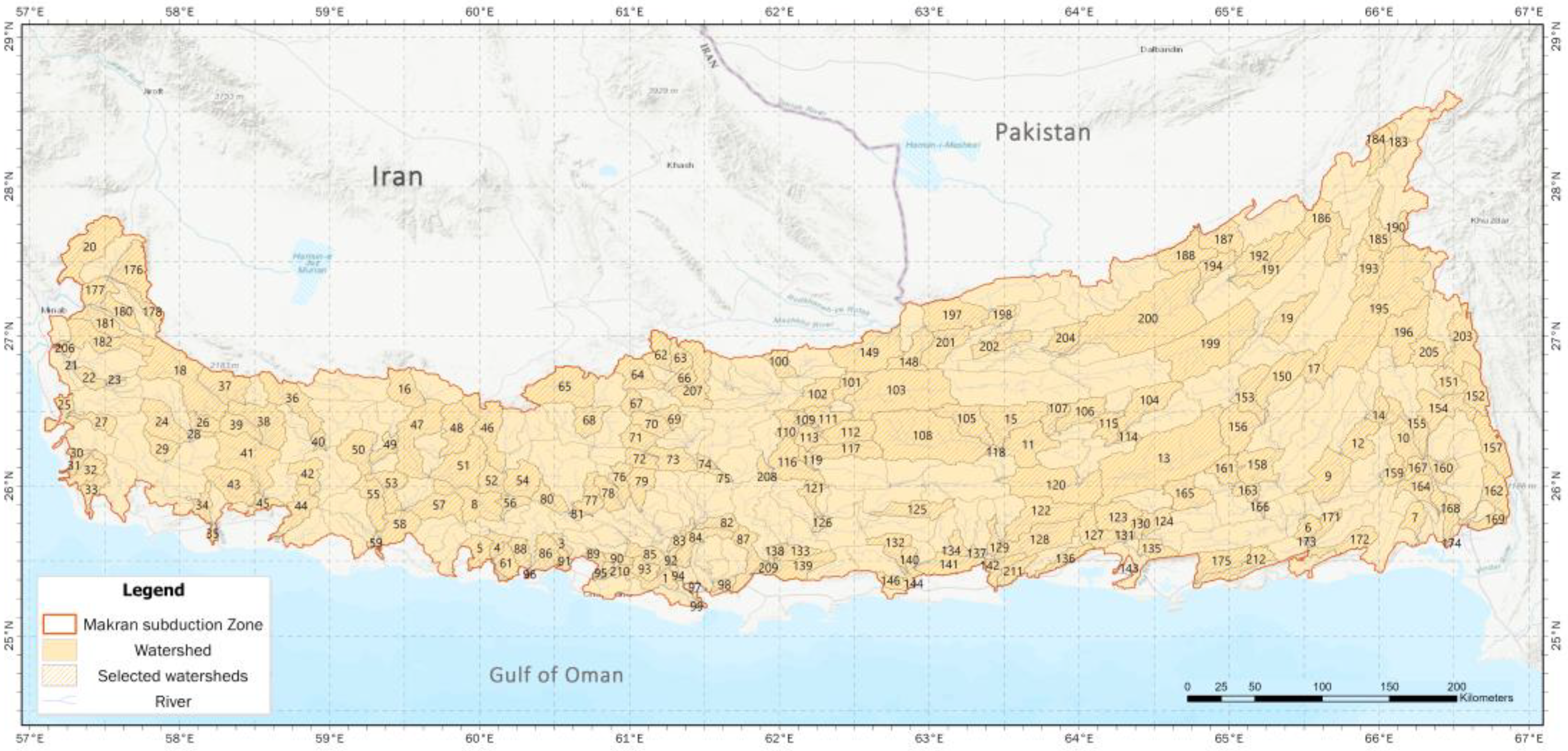
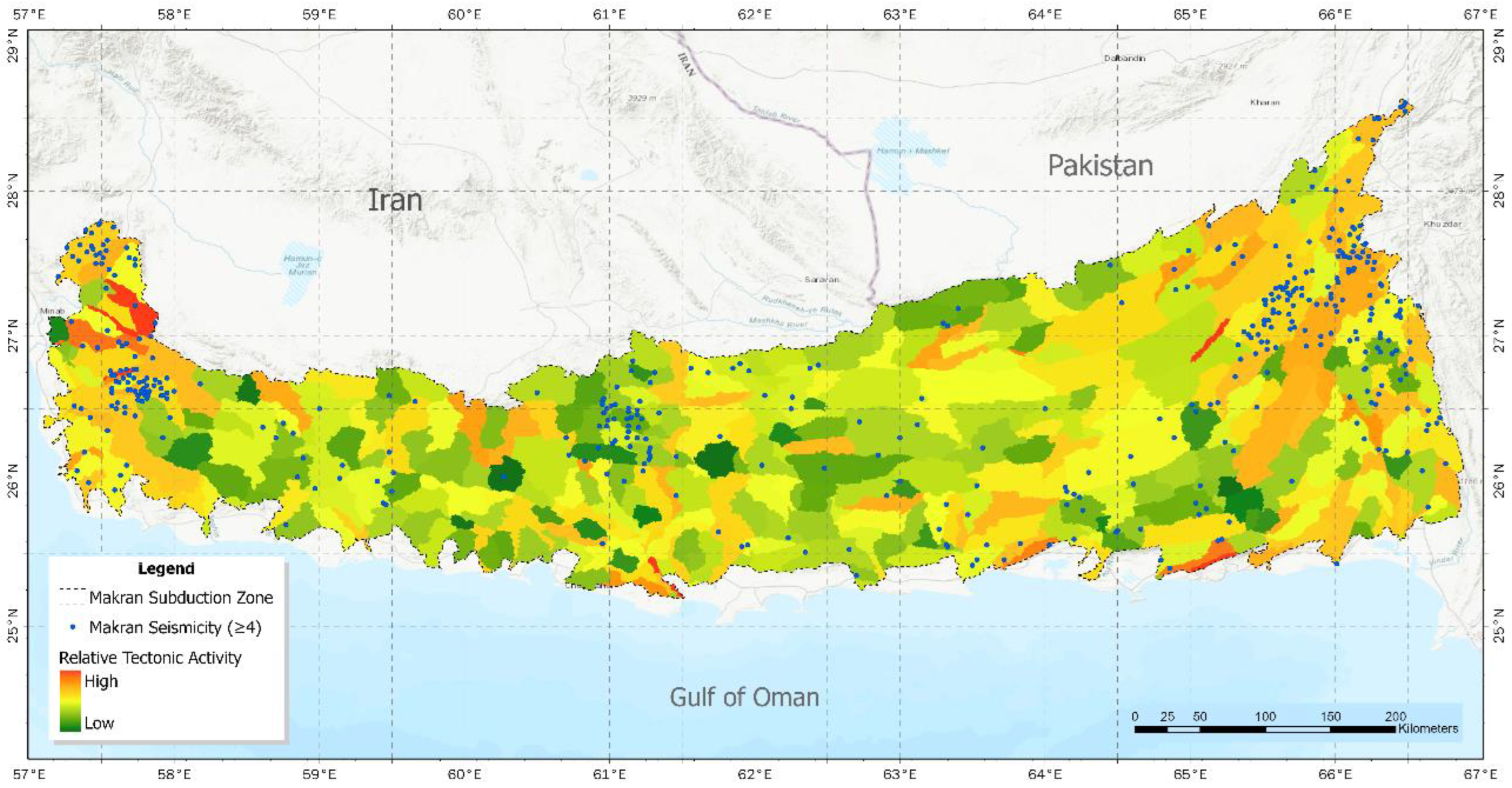
2.1. Study Area

The Makran subduction zone with east-west trending is located in southern Pakistan and Iran. This zone indicates a convergence zone where the Oman oceanic plate subducts beneath the Eurasian continental plate. The subduction probably started during the Late Cretaceous [30]. The western boundary of Makran is often called the Oman Line and Minab-Zendan Fault system, which runs northward and separates a highly seismic region in Zagros [31] from a region of low seismic activity in Makran to the east [32,33]. The eastern boundary of Makran is defined by a transfer zone consisting of three individual faults, namely the Ornach-Nal, Ghazaband, and Chaman faults [34,35].
In contrast to the majority of accretionary complexes in the world, the Makran accretionary wedge lacks an obvious trench [36]. The lack of a trench in this region may be because the angle of the subduction slab at the accretionary front is low, which may be caused by the presence of 7 km thick sediments with low compaction [37]. The seaward 70 km of the forearc comprises semi-consolidated and unconsolidated sediments with high pore fluid pressures and low seismic velocities. These sediments are capable of causing and failing large tsunamigenic slides [38].
The convergence rate decreases east to west along the Makran boundary [39]. In Makran, the average convergence rate is 4 cm/year, decreasing from 4.2 cm/year in the east to 3.65 cm/year in the west. Furthermore, GPS measurements suggest that the highest subduction rate of the Oman oceanic plate beneath the Eurasian plate occurs in the east at about 2.7 cm/year. In comparison, the lowest rate occurs in the west at about 1.95 cm/year [40]. Compared to other subduction zones, such as the Cascadia subduction zone at 35 mm/year [41], the Mexico subduction zone at 41 mm/year [42], the Sumatra subduction zone at 65 mm/year [43], the south Chile subduction zone at 70 mm/year [44], the Japan subduction zone at 80 mm/year [45], and the Tonga subduction zone at 160 mm/year [44], Makran is considered a relatively slow subduction zone.
Zarifi [46] states that the compressional stress direction along the Makran zone is rotating. The stress field in the eastern Makran is influenced by the collision between the Indian and Eurasian plates, while the western Makran stress field is affected by the Arabia-Eurasian collision. Eastern and western parts of the Makran subduction zone exhibit distinctive seismic behavior. The eastern region of Makran displays more seismic activity than the western region [38]. The plate boundary in western Makran lacks well-documented great instrumental and historical earthquakes. In contrast, eastern Makran was ruptured by thrust faulting during the 1945 earthquake and currently experiences earthquakes of varying magnitudes [38].
The main deformation phase from the Late Miocene to the Late Pliocene occurred by imbricating fans at the front of the Makran accretionary prism [47]. The seabed’s current geometry suggests that most of these imbricated fans remain active and that the accretionary prisms continue to be impacted by ongoing deformation from some branches of the imbricated fans. Following the Pliocene, the Makran coast and the mid-slope region experienced normal faulting, uplifting, and ductile flows [47].
The Makran subduction zone, like many other subduction zones around the world, has active mud volcanoes, some of which have formed along anticlinal axes [48]. As the largest mud volcanoes in the world [48], the mud volcanoes in Makran result from mud diapirism, providing evidence for the tectonic expulsion of mud and fluids seaward of the accretionary front. This confirms that tectonic forcing plays a significant role in forming mud volcanoes in Makran [49].

2.2. Extracting the Geomorphic Parameters

In this study, the morphotectonic zoning method was implemented in two steps. The watersheds of the research region were first determined using the Japan Aerospace Exploration Agency’s ALOS World 3D30m images (AW3D30), Ver.3.2 [50], with a resolution of 30 m (Figure 1). Numerous studies have demonstrated that AW3D30 DEM data can be compared to other open-source DEMs, such as SRTM and ASTER, with the advantage of being more accurate in delineating river basins and presenting drainage networks [51,52]. Next, ArcGIS Pro was used to evaluate the morphometric parameters and all physiographic indices to determine the watersheds with higher uplift. The eight indices employed in the morphotectonic process are shown in Figure 2.

2.3. Calculating Criterion Weights by FAHP

The Analytical Hierarchy Process (AHP) provides a systematic approach for evaluating complex decisions by combining qualitative and quantitative factors within a single framework, resulting in a prioritized list of alternatives [53]. Despite its widespread use, there have been concerns raised by researchers regarding certain limitations of the AHP, such as ambiguity in standardizing non-commensurate criteria (i.e., criteria that cannot be compared due to differences in size, type, or scale) and the influence of personal assessments [54]. These limitations can significantly impact the results of the AHP [55,56,57]. To address these issues, the Fuzzy Analytical Hierarchy Process (FAHP) has been developed to overcome the limitations and flaws of the AHP [58,59,60]. In this context, FAHP was employed to assess the weighting criteria related to morphotectonic zoning.
Mohebbi Tafreshi et al. [61] presented a fuzzy modelling method consisting of the following steps. The initial step in fuzzy models involves standardizing parameters using a fuzzy membership function. The experts’ opinions are utilized to assign fuzzy values to raw input values using a transformation function, where values close to 1 are deemed more suitable for the desired outcome, and values close to 0 are considered less suitable. The fuzzy logic extension of the ArcGIS Pro 2.8 software (version 10.8) offers various fuzzy membership functions. The selection of the fuzzification function is based on the nature, significance, and relation of each criterion to the goal. For this preliminary analysis, the Linear and Gaussian functions were chosen from the seven available fuzzy membership functions to standardize the factors.
The fuzzy linear transformation function applies a linear transformation between the minimum and maximum values specified by the user. Any value below the minimum will be assigned a 0 (definitely not a member), and any value above the maximum will be assigned a 1 (definitely a member). On the other hand, the fuzzy Gaussian function transforms the original values into a normal distribution [62].
The process of identifying the critical factors in the morphotectonic analysis was initiated by conducting a literature review, which resulted in identifying the most important indices, as shown in Figure 2. The relative significance of each parameter was then estimated through the use of the Analytic Hierarchy Process (AHP) and a constructed pairwise comparison matrix (8 × 8) based on the input factors, as determined by Saaty’s scale (Table 1). It is worth noting that the likelihood of inconsistencies in pairwise comparisons increases with the number of comparisons made, as stated in reference [63]. To account for this, AHP incorporates a consistency index (CI) to evaluate the calculated weight matrix. The weight is deemed acceptable if the CI is less than 10% (Table 2). Finally, the calculated weights were normalized to a scale between 0 and 1 to facilitate the integration of the weighted map layers.

2.4. Description and Application of the Criterion

Morphometric analysis of watersheds as a prerequisite of hydrological studies would be a valuable method to make informed management choices based on a more comprehensive view of the drainage network’s behavior and the morphology of the watershed.
In this study, eight linear and area-based indices of watersheds are evaluated. These indices provide a broad overview of the drainage basin network with regard to morphology and relief. These indices assess the stream network’s complexity, texture, and distortion due to neotectonic disturbances [64]. The extracted values are valuable in understanding the development of the drainage network concerning lithology and landscape. These indices are explained in detail as follows.

2.4.1. Hypsometric Integral (Hi)

The hypsometric curve represents the elevation distribution concerning the drainage area at various levels, including regional and continental scales [65,66]. The hypsometric integral (Hi) calculates the uneroded volume of a basin by determining the area under the hypsometric curve [67]. This can be computed through Equation (1).
Hi = H a v g H m i n H m a x H m i n
A value of Hi greater than 0.6 signifies a tectonically active region with significant uplift and steep topography [68,69,70]. On the other hand, a mature drainage basin exhibits a moderate-to-low Hi value [71]. In this study, a fuzzy linear membership function was utilized, where a Hi value of 0.65 was assigned the highest weight, and the weight progressively decreased to zero as the Hi value approached 0.04.

2.4.2. Basin Shape (Bs)

The shape of drainage basins in active tectonic zones is generally elongated, but over time it tends to become more circular [67]. The Basin Shape Index (Bs) is calculated using Equation (2) [72,73] to describe this change.
Bs = Bl Bw
This index is based on the length (Bl) and width (Bw) of the basin, measured from the headwater to the mountain ridge and at the broadest point, respectively. These values are calculated using the minimum bounding geometry script. Basins that have lower Bs values are considered more circular in shape and are usually associated with low tectonic activity. On the other hand, steep basins that have high tectonic activity are elongated [29,74]. The most significant weight is assigned to Bs values around 7.9 using the increasing fuzzy linear membership, and as the Bs value decreases to 0.16, the weight decreases until it reaches zero.

2.4.3. Circularity Basin (Cb)

The concept of the circulatory basin (Cb) was introduced by Miller [75] and Strahler [76] and it is defined as the ratio of the area of the basin (A) to the area of a circle with the same perimeter as the basin Equation (3).
Cb = 4 π A P 2
where A represents the area of the basin and P is the basin’s perimeter. The circularity index ranges from 0 for a straight line to 1 for a perfect circle. The more circular the shape of the basin, the higher the value of Cb. Factors such as the length, frequency of streams (Fs), geological structures, land cover, climate, relief, and slope of the basin all play a role in determining the circulatory ratio, making it a key factor in determining the stage of a basin. Low, medium and high Cb values correspond to a basin’s youthful, mature, and ageing periods [77,78]. In this context, the decreasing fuzzy linear membership assigns the lowest weight to a Cb value close to 0.3, and as the Cb value decreases to 0.03, the weight also decreases until it reaches zero.

2.4.4. Elongation Ratio (Er)

The elongation ratio (Er) measures the shape of a drainage basin, representing the ratio of the diameter of a circle with the same area as the basin to the basin’s length [79]. A value of 1 indicates a perfectly circular shape, while a lower value suggests a more elongated and tectonically impacted basin (as described in Equation (4)).
Er = 2 A π L
In this study, the highest and lowest Er values were found to be 0.17 and 0.06, respectively. Using the increasing fuzzy linear membership, the highest weight was assigned to an Er value close to 0.17, steadily decreasing as the Er value decreased to 0.06 and reached zero.

2.4.5. Ruggedness Number (Rn)

The Ruggedness Index, which combines two factors: relief (H) and drainage density (Dd), indicates the steepness and length of slopes. The calculation of the Ruggedness Index is carried out using Equation (5a–c).
Rn = Dd   · H
Dd =   Li   A
H = Hmax – Hmin
Where Li is the length of the river, and A is the area of the watershed. Hmax and Hmin are the highest and lowest elevations of the watershed. The Rn close to 473 is allocated the highest weight utilizing the rising fuzzy linear membership. As the Rn value approaches 1, the weight drops until it reaches zero.

2.4.6. River Sinuosity (Rs)

The morphology of rivers that interact with an active fault zone tend to become uneven due to changes in slope and variations in curvature, leading to increased meandering [80]. Hence, the sinuosity of a river (Rs) can be a valuable indicator of tectonic activity in a drainage basin. A highly sinuous river suggests stability, while a straight river profile suggests ongoing tectonic activity. The formula in Equation (6) can be used to calculate the sinuosity of a river, where c represents the channel length, and v represents the straight length of the valley. Utilizing a decreasing fuzzy linear membership, the highest weight is assigned to the Rs value closest to 1.03, while the weight decreases as the Rs value approaches 2.58.
Rs = C V

2.4.7. Compactness Coefficient (Cc)

The compactness coefficient, also known as the Gravellus Index, evaluates the basin’s shape irregularity. The more irregular the shape, the higher the value of Cc [81]. This value can be a good indicator of the area’s tectonic activity level Equation (7).
Cc = 0.2821 P A 0.5
where P is the perimeter and A is the area of the watershed. With the use of increasing fuzzy linear membership, a Cc value close to 5.03 is given the lowest weight. As the Cc value decreases to 1.83, the weight decreases until it reaches zero.

2.4.8. Form Factor (Ff)

As Horton [11] defined, the form factor represents the relationship between a basin’s area and length, squared. The equation for calculating the form factor is shown in Equation (8).
Ff = A L b 2
Here, A is the basin area in square kilometers, and L b 2  is the square of the basin length. A perfectly circular basin will have a form factor value lower than 0.78. Basins with a lower form factor are considered to be more elongated and potentially influenced by tectonic activity. Using the decreasing fuzzy linear membership, a form factor value close to 0.61 will be given the lowest weight. As the form factor decreases to 0.05, the weight will increase until it reaches one.

2.5. Machine Learning Algorithms

Traditionally, geological research has faced challenges with data sources that are complex and imprecise due to the size and complexity of geological objects [82]. However, with advancements in science and technology, new methods have emerged that enhance the precision of geological data and increase the amount of available information.
Artificial intelligence (AI) is a field within computer science that focuses on developing intelligent systems created by humans. It can be separated into two types: strong AI and weak AI. Weak AI views the creation of reasoning and problem-solving machines as impossible, while strong AI aims to build machines with the ability to think and make decisions. The study of AI encompasses various areas, such as expert systems, machine learning, natural language processing, computer vision, and recommendation systems. Machine learning explicitly explores how computer systems can improve automatically through experience and the fundamental laws that govern all learning systems, including humans, organizations, and computers.
Machine learning algorithms allow us to gain new insights and capabilities. The advent of deep learning has revolutionized the field of AI by addressing the challenges faced in traditional machine learning, such as limited model options, time-consuming training processes, and the complexity of determining model parameters. As a result, deep learning has become a pivotal area of AI advancement.
Representation learning enables machines to automatically identify patterns in raw data and learn the necessary representations for detection or classification. Deep learning methods are a type of representation learning that involve multiple levels of abstraction created by combining simple, nonlinear modules. As these modules are layered, increasingly complex functions can be learned and implemented.
The advancement of big data and AI has opened new opportunities in the field of geology in recent years. Thanks to increased computing power, particularly the progress in GPU technology, the limitations of big data and AI in terms of computing have been significantly reduced. This expands the potential applications and growth prospects of geology. AI is commonly utilized for geological surveys and resource exploration, such as mineral recognition and geochemical anomaly detection. This article delves into the topic of big data and AI in geology.

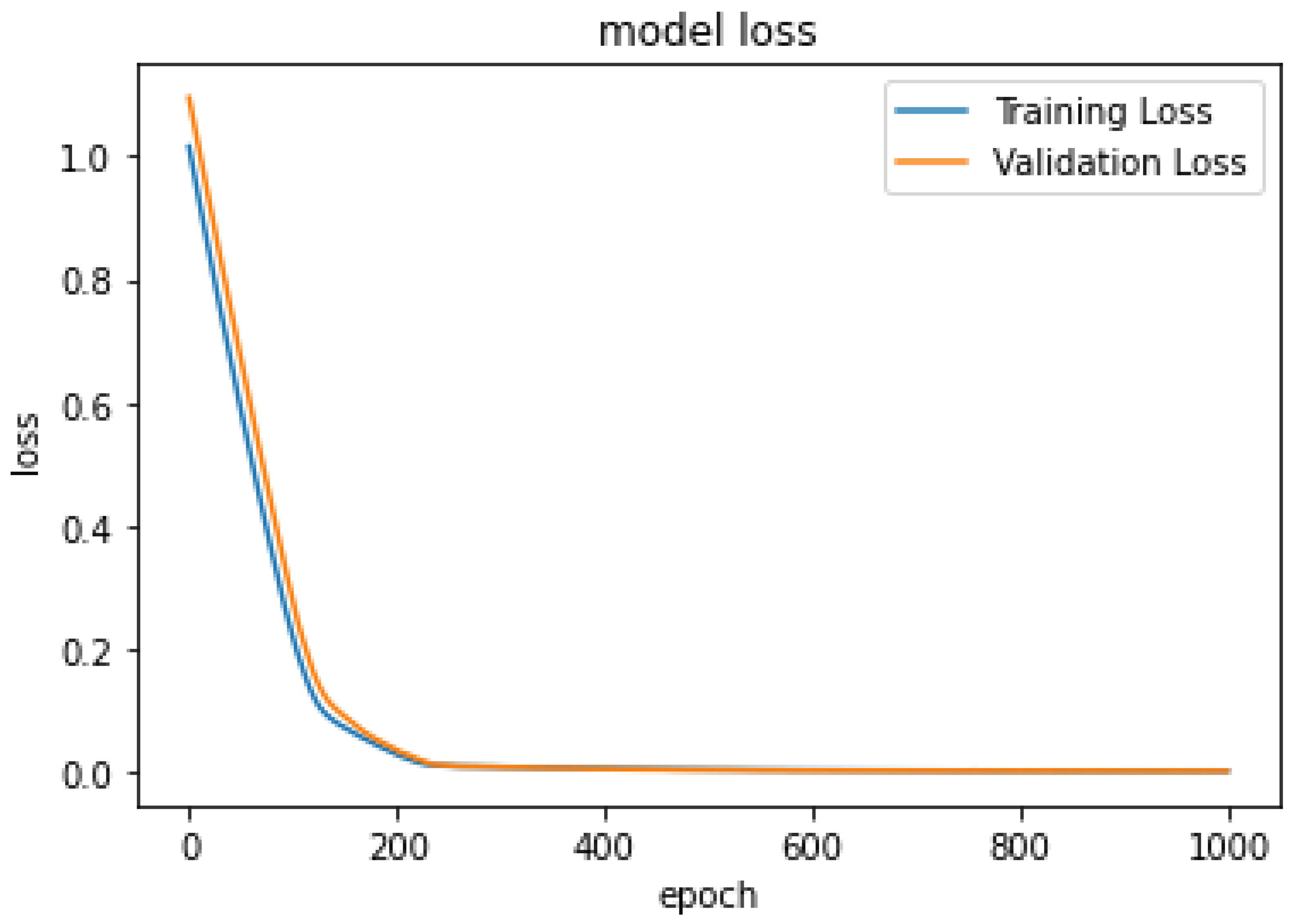
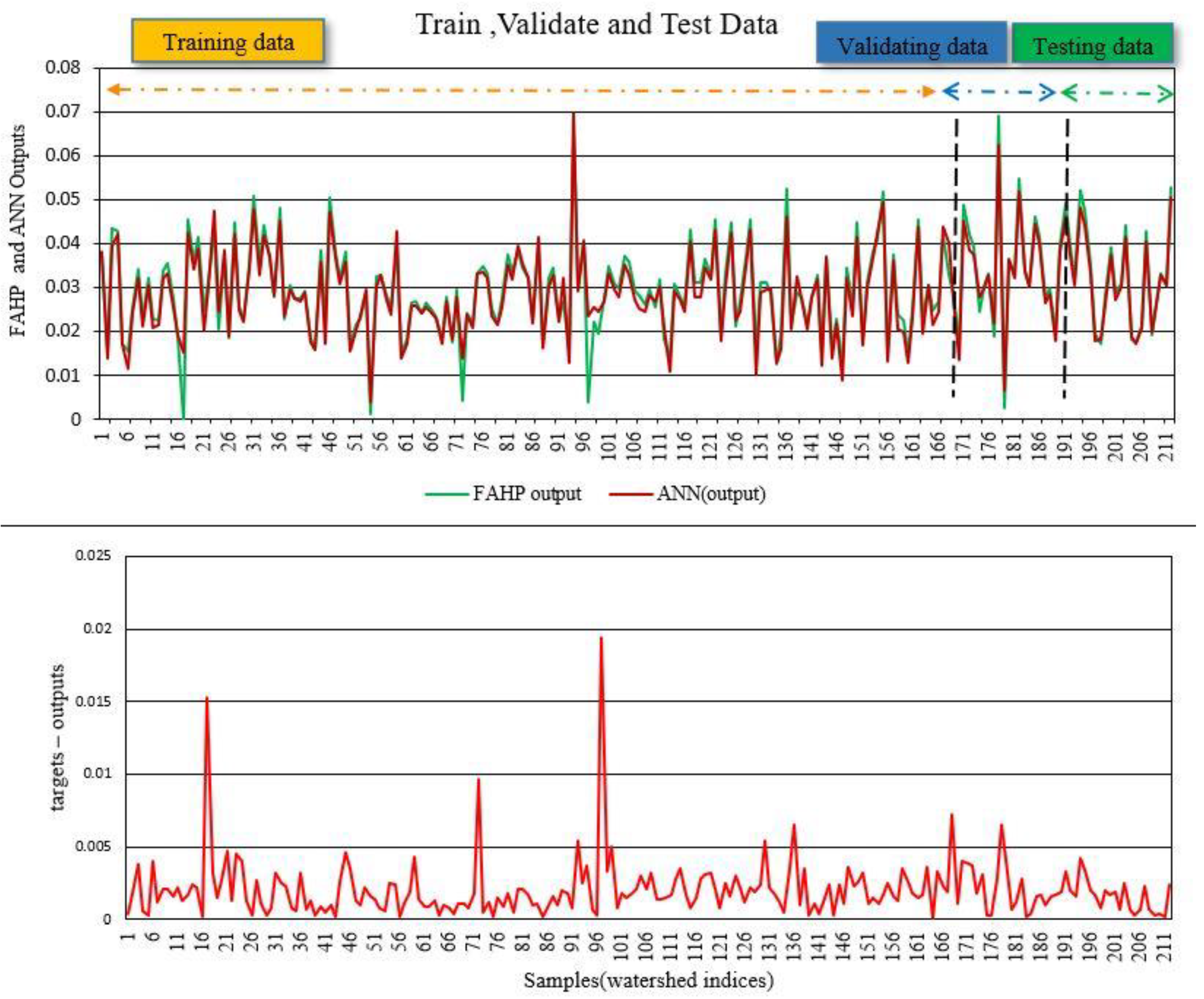
2.5.1. Artificial Neural Networks (ANNs)

Artificial Neural Networks (ANNs) are computational systems that draw inspiration from functioning biological nervous systems such as the human brain. ANNs comprise many interconnected computational nodes, called neurons, that work together to learn from inputs and optimize the output.
The input, typically a multidimensional vector, is fed into the input layer and distributed to the hidden layers. These layers make decisions based on the previous layer and assess the impact of random changes on the final output, a process referred to as learning. When multiple hidden layers are stacked, it is called deep learning. ANNs have several key features, including the ability to learn and adapt, generalize information, and process and analyze information uniformly and with error tolerance. These features make ANNs powerful tools for pattern recognition, classification, and nonlinear function estimation.
Activation functions are used in ANNs to transform the input into an output, which is then supplied as the input to the next layer. The weights of the connections between neurons in the layers are adjusted during the training phase, allowing the network to learn the patterns between inputs and outputs. ANNs can be divided into two learning models: supervised and unsupervised. In supervised learning, the network is trained with proper outputs for each input pattern. The weights are adjusted to minimize the error between the network output and the actual value. In unsupervised learning, the network discovers the relationship between the data patterns without needing actual responses.
ANNs can also be divided into two categories: recurrent and feed-forward networks. Recurrent networks have a feedback loop, while feed-forward networks do not. The neurons in each layer provide information to both the previous and the subsequent layers.
The ANNs offer these hypotheses:
  • Data processing occurs in the units known as neurons. The neurons (or artificial neurons) present a model of brain neurons.
  • The exchange of data is facilitated through communication between neurons.
  • There is a weight for communicative ways between neurons.
  • Every neuron utilizes a nonlinear function to process its inputs (weighted data), producing a specific output [82].
It is possible to identify a neural network via the communicative model between different layers of the network, the number of layers, the number of neurons, the neuron’s operational function, and the learning algorithm. However, no general principle is available regarding the standard size of the network components. It is an innovative approach in most cases where the multilayered networks have a different amount of neurons in each layer, and different activation functions and various learning rates do the training of these networks. Then, it is followed by a selection of the best network. The network training in the learning phase takes place via the adjustment of weights so that outputs can be predicted or classified based on a set of inputs [83].
In this paper, the input parameters of the neural network included Basin Shape, Circularity Basin, Coefficient Compactness, Elongation Basin, Form Factor, Hypsometric Integral, River Sinuosity, Drainage Density, and Number Ruggedness, and the FAHP outputs were considered as the network output parameters. The data on these parameters were divided into training, testing, and data validation. A total of 80% of these data were used for training, 10% of data for validation and the other 10% for testing.

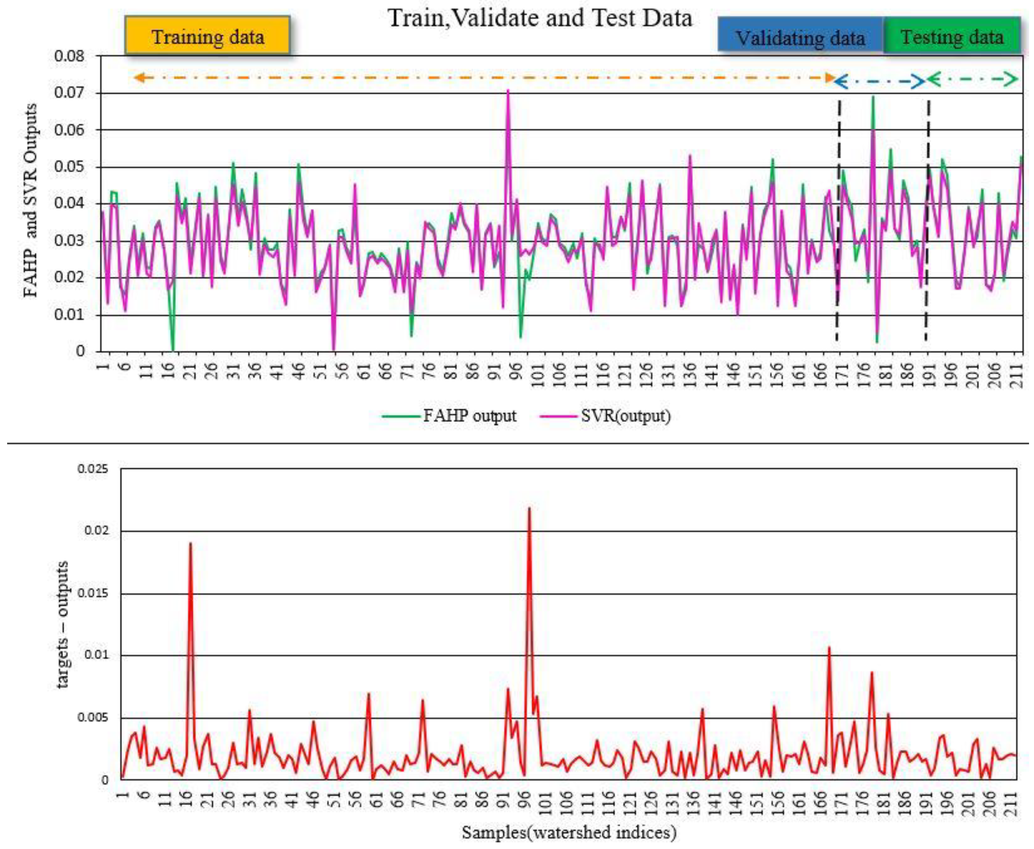
2.5.2. Support Vector Regression (SVR)

Considering a data set with N elements Xi ,   yi i = 1 N , where Xi = [x1,i, …, xn,i] ∈ R n and Xi represents the ith element in a space with n dimensions, yi (yi ∈ R) indicates the actual value for Xi, the definition of a nonlinear function is as follows: φ: R n → Rnh. For mapping the entry data, Xi represents an R nh space of high dimension known as feature space, which specifies the nonlinear transformation φ. Hence, a linear function f in a high-dimensional space, and consequently, the entry data, Xi can be related to output yi. Equation (9) presents the linear function, i.e., SVR.
f X = W T · φ X + b
where b R and W R n , and f X is the foretold value. As indicated in Equation (10), the empirical risk is minimized by the SVR.
R reg f = C i = 1 N Θ ε y i f X i + 1 2 || W T ||
where the cost function is represented by Θε(yi − f(Xi)), regarding the ε-SVR, as shown in Equation (11), a loss function ε-insensitive is utilized:
Θ ε y f X = y f X ε I f y f X ε   0 I n   a n o t h e r   c a s e
The nonlinear function φ is determined using Θε in the Rnh space for finding a function with the ability to fit present training data with a deviation equal to or below ε. Using the mentioned function, the training error is minimized between the data training, and Equation (12) provides the function ε-insensitive [84].
min W , b , ξ * , ξ R reg ( W , ξ * , ξ ) = 1 2 W T W + C i = 1 N ( ξ i * + ξ i )
The training errors of f(X) and Y are punished by Equation (12) via the function ε-insensitive. Using the parameter C, the compromise between the points meeting condition |f(X) − y| ≥ ε in Equation (11) and the model complexity (vector W) is determined. With C → ∞, a small model margin is observed that is adjusted to the data. When C → 0, there is a large model margin, which is why it softens. Lastly, ξi represents errors more minor than −ε and ξi indicates training errors larger than ε.
For solving the regression problem, the internal product of Equation (9) can be replaced by kernel K() functions. Thus, this operation can be performed in a higher dimension by low-dimensional space data input regardless of knowledge of the transformation φ [85].

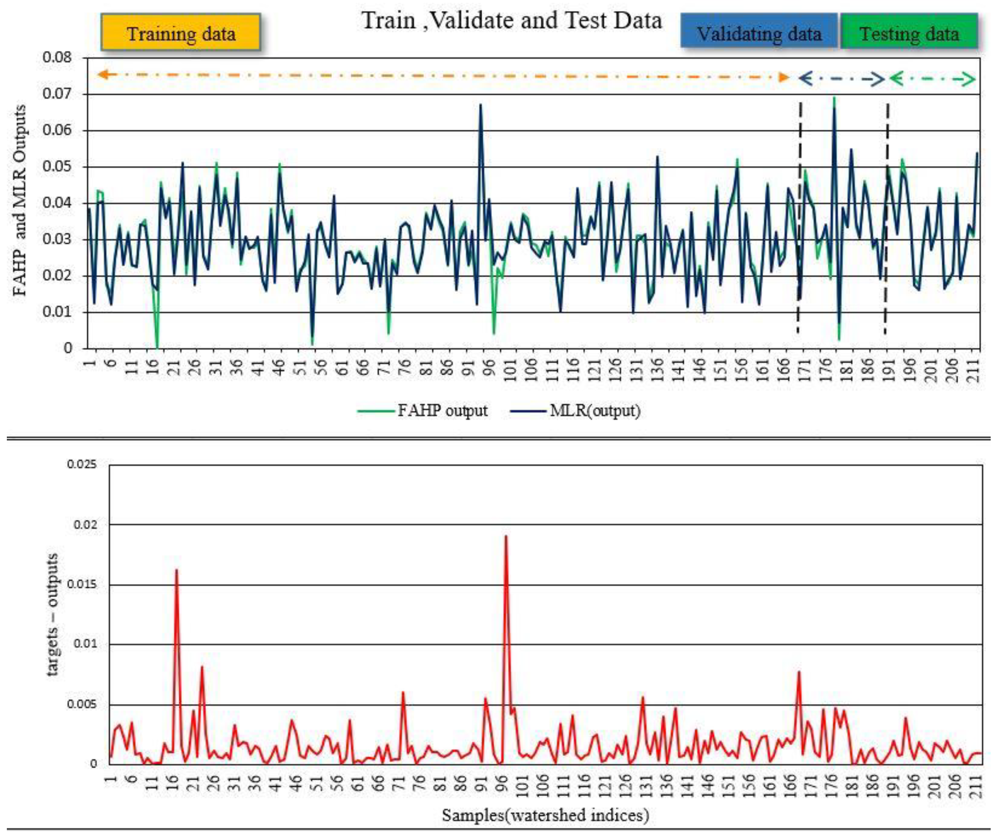
2.5.3. Multivariate Linear Regression (MLR)

The regression method is applied to two theories. Firstly, regression analysis is typically utilized for prediction and forecasting, and its application significantly overlaps the machine learning field. Secondly, it is possible to use regression analysis sometimes for determining causal relationships between the dependent and independent variables. Regression alone presents just relationships between a fixed dataset of different variables and a dependent variable.
Based on the regression models, the dependent variables are predicted by the independent variables. The value of the dependent ‘y’ variable is estimated by regression analysis because of the range of independent variable ‘x’ values. This articlediscusses polynomial and linear regression, which fit better into the predictive model. Regression could be multiple regression or a simple linear regression [86].
Simple linear regression is a statistical method used to model the relationship between a dependent variable and a single independent variable. An equation represents it, y = β0 + β1x + ε, where y is the dependent variable, x is the independent variable, β0 and β1 are coefficients, and ε represents the error term. The goal of simple linear regression is to determine the strength and direction of the relationship between the dependent and independent variables and estimate the effect of the independent variable on the dependent variable [86].
Multivariate linear regression is a statistical method for predicting the result of an answer variable, which uses some explanatory variables, as shown in Equation (13). Multiple Linear Regression (MLR) aims to establish a linear association between the dependent variable y and one or more independent variables x, which will then be analyzed.
  β ^ = X T X 1 X T y

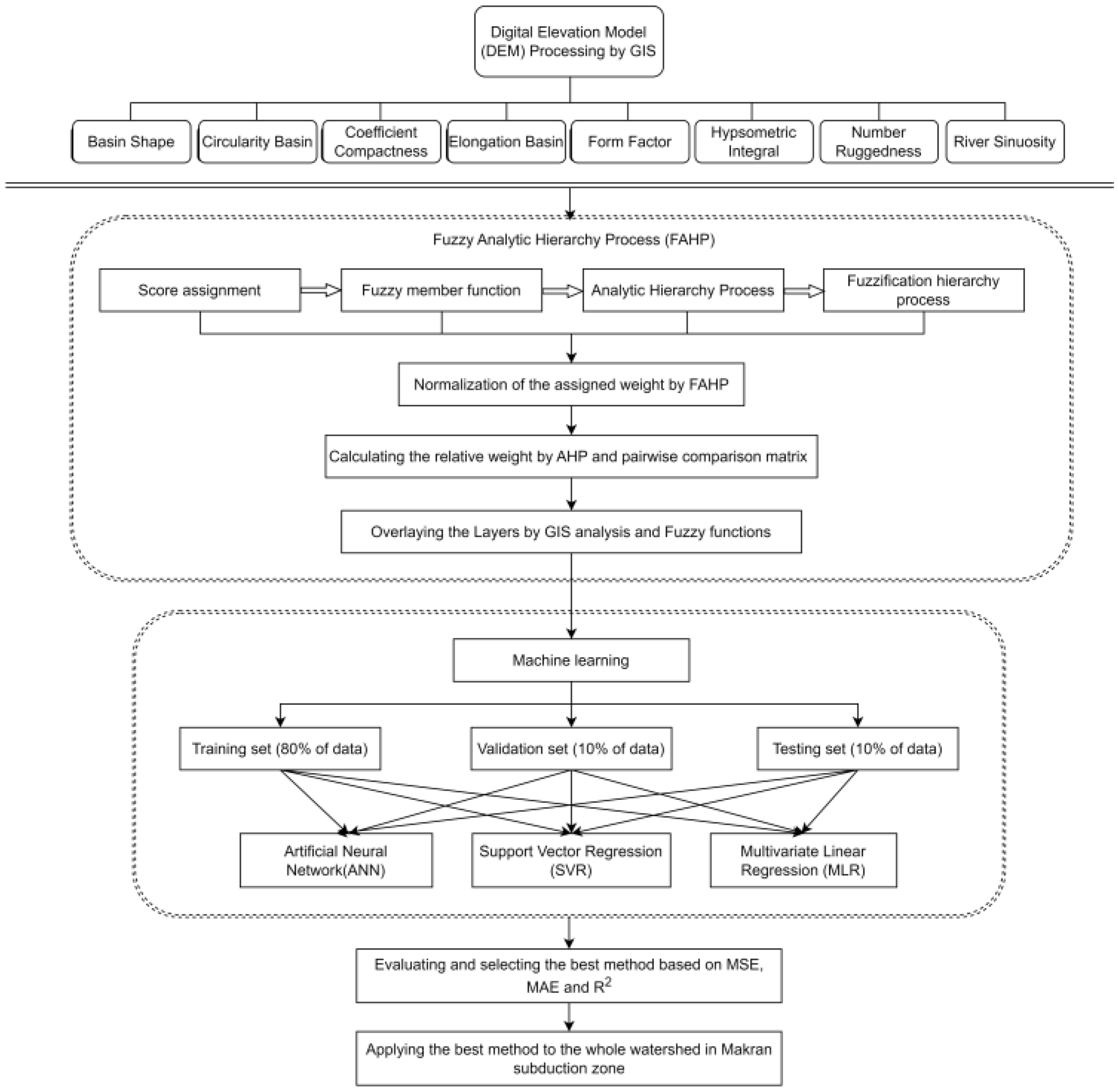
2.6. Integrating the FAHP and ML Algorithms

We first used the FAHP model to generate a target database suitable for our ML. This database served as the basis for training and testing the algorithms. Next, we randomly selected 212 out of 423 watersheds across our study area for training and testing the algorithms. By randomly selecting the watersheds, we ensured a representative sample of the study area. Here, raw data from eight different morphometric indices were used to train and test the machine learning algorithms, as shown in Figure 2. These indices were selected based on their relevance and importance in the morphotectonic characterization of watersheds. We then used these raw data as input features for the machine learning algorithms to generate predictions for the target database. Using a representative sample of the study area and including relevant input features, we aimed to create a distinct training network and improve the accuracy and precision of our predictions and our cost-effectiveness. Three distinct ML algorithms, namely, ANNs, SVR, and MLR methods, were employed for each set. It is important to note that the training and testing set includes 212 watershed indices. After optimizing and obtaining the best algorithms using statistical equations, the method was generalized for the whole domain.
To assess the effectiveness of the ANNs, SVR, and MLR techniques, Mean Squared Error (MSE), Mean Absolute Error (MAE), and Correlation Coefficient (R2) were utilized as performance metrics. These metrics are described in Equation (14a–c) [82].
MSE = 1 N i = 1 N y i y ^ i 2
MAE = 1 N i = 1 N y i y ^   i
R 2 = 1 i y i   y ^   i 2 i y i   y ¯   2
We used ANN for regression here and utilized the supervised method. Also, we use L2 (ridge) regularization to avoid overfitting. To have a faster converging, we need zero-centered data points, and each dimension should be scaled according to its standard deviation. Thus we normalize our data.
Figure 3 shows the performance of the ANN method for the training and validation sets. From epoch 200 and on, the trend was deemed acceptable. After completing the learning process, the ANN model demonstrated high accuracy with an R2 value of 0.974, MSE of 4.14 × 10⁻⁶, and MAE of 0.00151.
After developing and training the SVR model with the value of 0.947, MSE and MAE obtained 8.12 × 10⁻⁶ and 1.94 × 10⁻³, respectively.
After developing and training the MLR model with the value of 0.967, MSE and MAE obtained 5.06 × 10⁻⁶ and 1.61 × 10⁻³, respectively.
According to the simulation results obtained, there is a good agreement between the results obtained from ANN, SVR and MLR models but ANN model outperformed the other models. All three algorithms demonstrated similar error patterns in our study, with samples 16 and 96 displaying particularly large prediction errors. We have further investigated the reason for these high prediction errors and found that the location of these two samples may have contributed to the discrepancies. Specifically, sample 16 is located in the northernmost part of the study area, where geological and climatic conditions differ significantly from the rest of the watersheds. Similarly, sample 96 is situated in the southernmost part of the study area, which also has distinct geological and climatic conditions compared to the majority of the watersheds.
These differences in geological and climatic conditions may have played a role in the higher prediction errors observed for samples 16 and 96. Our findings suggest that when analyzing and predicting data in areas with distinct geological and climatic conditions, particular attention should be paid to samples that are situated in the outlier regions of the study area. By doing so, we may better understand and account for the differences in geological and climatic conditions and obtain more accurate predictions.
Overall, our study highlights the importance of considering the spatial distribution of data and the potential impact of varying geological and climatic conditions when making predictions. Further research may be necessary to determine how these findings can be applied in other contexts or how they can inform the development of more accurate predictive models.

3. Results and Discussion

ML techniques use algorithms to learn from data and make predictions or decisions without being explicitly programmed. Meanwhile, the fuzzy technique assigns degrees of truth to statements or rules, making it useful in assessing morphometry in watersheds where data such as rainfall patterns or soil properties can be difficult to quantify accurately. These techniques are useful in engineering problems where the relationship between input and output variables is complex and challenging to model analytically, such as landslides and mass movements [87,88].
However, both techniques have limitations in practical applications. Fuzzy logic relies heavily on expert knowledge to define rules and membership functions, resulting in models that are challenging to interpret and validate. ML techniques are limited by the quality and quantity of available data and the choice of algorithm and parameters used. Overfitting or underfitting data can result in poor predictive performance on new data. Successful application requires careful consideration of their limitations and appropriate use of available data and expertise.
Our study divided the dataset into three groups: a training dataset that accounted for 80% of the collected data, a validation dataset that accounted for 10%, and a testing dataset that comprised the remaining 10%. The performance of the machine learning methods on both the training and testing data is depicted in Figure 4, Figure 5 and Figure 6. These figures compared the target (FAHP output) and output (predicted by algorithms) values and calculated the model error. Numerical results closely matched those obtained from the ANN, SVR, and MLR methods (Table 3). However, the ANN model showed superior performance compared to the other methods.
We investigated the potential of coupled artificial intelligence algorithms and FAHP to predict the watershed’s behavior in response to the region’s tectonics. After selecting the best from among the ANN, SVR and MLR methods, the model was applied to whole watersheds in the Makran Subduction zone (Figure 7).
Mapping the results acquired by artificial intelligence algorithms for analog interpretation and comparing them with tectonic features and seismic events indicates the acceptable accuracy of the algorithms used. As shown in Figure 7, the findings measured for each watershed are illustrated in the range of low- to high levels of tectonic activity, which correlates well with the tectonic situation. On the west side of the figure, the location of the Minab fault zone is in good agreement with the area marked on the map as a zone with relatively high tectonic activity. Additionally, this region experiences the effects of two unique geological occurrences: the convergence of the Iranian and Arabian tectonic plates in the west and the subduction of the Oman sea plate beneath the Iranian continent in the east, both ongoing processes. On the eastern side of the region, it is observed that tectonic activity is estimated to be relatively high based on morphometric parameters.
This area aligns with the Chaman fault zone in Pakistan and marks the eastern boundary where the Oman oceanic plate is subducting beneath the Iranian continental plate. Moreover, instrumental epicenters also confirm the higher activity of this zone. The noteworthy point in this figure is the presence of instrumental epicenters in the central region, which are consistent with the results obtained using AI approaches, albeit with a slight shift to the left.
It is affected by the inclination of seismic faults, earthquakes, the geometry of the subducted oceanic plate, and instrumental error. The development of morphometric indicators can be affected by various factors, including geological heterogeneity, land use, and climate conditions. While high erosion rates in certain geological layers may contribute to the lack of clear development of tectonic indicators in some watersheds, it is important to note that this is only one potential explanation among many. Other factors, such as high levels of sedimentation, variations in precipitation patterns, and land use changes, could also contribute to the observed variability in technical indicator development. Additionally, interactions between multiple factors may contribute to the observed patterns.
Furthermore, it should be noted that seismic instrument data belong to only the last hundred years, whereas the morphometric features date back several million years which makes it more reliable. To better understand the underlying causes of the variability, it may be necessary to conduct further analyses that consider these different factors and potential interactions. It is also important to consider the limitations of the data and methods used in the study, as these may affect the accuracy and reliability of the technical indicators.

4. Conclusions

In conclusion, the morphometric analysis of watersheds in a region has the potential to reveal insights into long-term tectonic activity, and the present study aims to develop a novel approach to enhance this analysis. The proposed method leverages advanced machine learning techniques to reduce computational cost and time, especially in the case of large-scale regions. In this study, we examined the morphometry of watersheds in the Makran subduction zone using three artificial intelligence methods: ANN, SVR, and MLR. The results of our analysis indicate that the ANN method is the most accurate of the three, with a value of 0.974. The MSE and MAE values of the ANN method were also found to be lower compared to the other methods. Based on these findings, it can be concluded that the ANN approach can be effectively utilized in the morphometric analysis of watersheds and provides better results than previous techniques.

Author Contributions

Conceptualization, R.D. and M.Z.; methodology, M.Z. and V.N.; software, A.G.; validation, R.D., M.Z. and V.N.; formal analysis, A.R. (Ahmad Rashidi) and M.N.; investigation, S.S.; resources, R.D., M.Z. and A.R. (Ahmad Rashidi); data curation, R.D. and V.N.; writing—original draft preparation, R.D., M.Z., A.G. and V.N.; writing—review and editing, R.D., M.Z. and V.N.; supervision, R.D and A.R. (Amir Raoof); project administration, R.D. All authors have read and agreed to the published version of the manuscript.

Funding

This research received no external funding.

Data Availability Statement

Not applicable.

Conflicts of Interest

The authors declare no conflict of interest.

References

  1. Christophe, O.; Olaniyi Ti, D. Applications of Geographical Information Systems (GIS) for Spatial Decision Support in Eco-Tourism Development. Environ. Res. J. 2010, 4, 187–194. [Google Scholar] [CrossRef]
  2. Segura, F.S.; Pardo-Pascual, J.E.; Rosselló, V.M.; Fornós, J.J.; Gelabert, B. Morphometric Indices as Indicators of Tectonic, Fluvial and Karst Processes in Calcareous Drainage Basins, South Menorca Island, Spain. Earth Surf. Process. Landf. 2007, 32, 1928–1946. [Google Scholar] [CrossRef]
  3. Juez, C.; Garijo, N.; Hassan, M.A.; Nadal-Romero, E. Intraseasonal-to-Interannual Analysis of Discharge and Suspended Sediment Concentration Time-Series of the Upper Changjiang (Yangtze River). Water Resour. Res. 2021, 57, e2020WR029457. [Google Scholar] [CrossRef]
  4. Mesa, L.M. Morphometric Analysis of a Subtropical Andean Basin (Tucumán, Argentina). Environ. Geol. 2006, 50, 1235–1242. [Google Scholar] [CrossRef]
  5. Kermani, A.F.; Derakhshani, R.; Bafti, S.S. Data on Morphotectonic Indices of Dashtekhak District, Iran. Data Brief. 2017, 14, 782–788. [Google Scholar] [CrossRef]
  6. Rahbar, R.; Bafti, S.S.; Derakhshani, R. Investigation of the Tectonic Activity of Bazargan Mountain in Iran. Sustain. Dev. Mt. Territ. 2017, 9, 380–386. [Google Scholar] [CrossRef]
  7. Aher, P.D.; Adinarayana, J.; Gorantiwar, S.D. Quantification of Morphometric Characterization and Prioritization for Management Planning in Semi-Arid Tropics of India: A Remote Sensing and GIS Approach. J. Hydrol. 2014, 511, 850–860. [Google Scholar] [CrossRef]
  8. Salvany, J.M. Tilting Neotectonics of the Guadiamar Drainage Basin, SW Spain. Earth Surf. Process. Landf. 2004, 29, 145–160. [Google Scholar] [CrossRef]
  9. Javed, A.; Khanday, M.Y.; Rais, S. Watershed Prioritization Using Morphometric and Land Use/Land Cover Parameters: A Remote Sensing and GIS Based Approach. J. Geol. Soc. India 2011, 78, 63–75. [Google Scholar] [CrossRef]
  10. Rashidi, A.; Abbassi, M.-R.; Nilfouroushan, F.; Shafiei, S.; Derakhshani, R.; Nemati, M. Morphotectonic and Earthquake Data Analysis of Interactional Faults in Sabzevaran Area, SE Iran. J. Struct. Geol. 2020, 139, 104147. [Google Scholar] [CrossRef]
  11. Horton, R.E. Erosional Development of Streams and Their Drainage Basins; Hydrophysical Approach to Quantitative Morphology. Geol. Soc. Am. Bull 1945, 56, 275–370. [Google Scholar] [CrossRef] [Green Version]
  12. Strahler, A.N. Hypsometric (Area-Altitude) Analysis of Erosional Topography. Geol. Soc. Am. Bull 1952, 63, 1117–1142. [Google Scholar] [CrossRef]
  13. Hack, J.T. Studies of Longitudinal Stream Profiles in Virginia and Maryland. In USGS Professional Paper; US Government Printing Office: Washington, DA, USA, 1957; Volume 294. [Google Scholar]
  14. Ribolini, A.; Spagnolo, M. Drainage Network Geometry versus Tectonics in the Argentera Massif (French-Italian Alps). Geomorphology 2008, 93, 253–266. [Google Scholar] [CrossRef]
  15. Bemis, S.P.; Micklethwaite, S.; Turner, D.; James, M.R.; Akciz, S.T.; Thiele, S.; Bangash, H.A. Ground-Based and UAV-Based Photogrammetry: A Multi-Scale, High-Resolution Mapping Tool for Structural Geology and Paleoseismology. J. Struct. Geol. 2014, 69, 163–178. [Google Scholar] [CrossRef]
  16. Ozdemir, H.; Bird, D. Evaluation of Morphometric Parameters of Drainage Networks Derived from Topographic Maps and DEM in Point of Floods. Environ. Geol. 2009, 56, 1405–1415. [Google Scholar] [CrossRef]
  17. Chorowicz, J.; Dhont, D.; Gündogdu, N. Neotectonics in the Eastern North Anatolian Fault Region (Turkey) Advocates Crustal Extension: Mapping from SAR ERS Imagery and Digital Elevation Model. J. Struct. Geol. 1999, 21, 511–532. [Google Scholar] [CrossRef]
  18. Azarafza, M.; Azarafza, M.; Akgün, H.; Atkinson, P.M.; Derakhshani, R. Deep Learning-Based Landslide Susceptibility Mapping. Sci. Rep. 2021, 11, 24112. [Google Scholar] [CrossRef]
  19. Ghosh, M.; Gope, D. Hydro-Morphometric Characterization and Prioritization of Sub-Watersheds for Land and Water Resource Management Using Fuzzy Analytical Hierarchical Process (FAHP): A Case Study of Upper Rihand Watershed of Chhattisgarh State, India. Appl. Water Sci. 2021, 11, 17. [Google Scholar] [CrossRef]
  20. Kumar, R.; Dwivedi, S.B.; Gaur, S. A Comparative Study of Machine Learning and Fuzzy-AHP Technique to Groundwater Potential Mapping in the Data-Scarce Region. Comput. Geosci. 2021, 155, 104855. [Google Scholar] [CrossRef]
  21. Zaresefat, M.; Ahrari, M.; Reza Shoaei, G.; Etemadifar, M.; Aghamolaie, I.; Derakhshani, R. Identification of Suitable Site-Specific Recharge Areas Using Fuzzy Analytic Hierarchy Process (FAHP) Technique: A Case Study of Iranshahr Basin (Iran). Air Soil Water Res. 2022, 15, 11786221211063849. [Google Scholar] [CrossRef]
  22. Zaresefat, M.; Derakhshani, R.; Nikpeyman, V.; GhasemiNejad, A.; Raoof, A. Using Artificial Intelligence to Identify Suitable Artificial Groundwater Recharge Areas for the Iranshahr Basin. Water 2023, 15, 1182. [Google Scholar] [CrossRef]
  23. Önüt, S.; Efendigil, T.; Soner Kara, S. A Combined Fuzzy MCDM Approach for Selecting Shopping Center Site: An Example from Istanbul, Turkey. Expert. Syst. Appl. 2010, 37, 1973–1980. [Google Scholar] [CrossRef]
  24. Bui, D.T.; Shahabi, H.; Shirzadi, A.; Chapi, K.; Pradhan, B.; Chen, W.; Khosravi, K.; Panahi, M.; Bin Ahmad, B.; Saro, L. Land Subsidence Susceptibility Mapping in South Korea Using Machine Learning Algorithms. Sensors 2018, 18, 2464. [Google Scholar] [CrossRef] [Green Version]
  25. Corsini, A.; Cervi, F.; Ronchetti, F. Weight of Evidence and Artificial Neural Networks for Potential Groundwater Spring Mapping: An Application to the Mt. Modino Area (Northern Apennines, Italy). Geomorphology 2009, 111, 79–87. [Google Scholar] [CrossRef]
  26. Naghibi, S.A.; Pourghasemi, H.R. A Comparative Assessment between Three Machine Learning Models and Their Performance Comparison by Bivariate and Multivariate Statistical Methods in Groundwater Potential Mapping. Water Resour. Manag. 2015, 29, 5217–5236. [Google Scholar] [CrossRef]
  27. Arabameri, A.; Saha, S.; Roy, J.; Chen, W.; Blaschke, T.; Bui, D.T. Landslide Susceptibility Evaluation and Management Using Different Machine Learning Methods in the Gallicash River Watershed, Iran. Remote Sens. 2020, 12, 475. [Google Scholar] [CrossRef] [Green Version]
  28. Sarangi, A.; Madramootoo, C.A.; Enright, P.; Prasher, S.O.; Patel, R.M. Performance Evaluation of ANN and Geomorphology-Based Models for Runoff and Sediment Yield Prediction for a Canadian Watershed. Curr. Sci. 2005, 89, 2022–2033. [Google Scholar]
  29. El Hamdouni, R.; Irigaray, C.; Fernández, T.; Chacón, J.; Keller, E.A. Assessment of Relative Active Tectonics, Southwest Border of the Sierra Nevada (Southern Spain). Geomorphology 2008, 96, 150–173. [Google Scholar] [CrossRef]
  30. Dykstra, J.D.; Birnie, R.W. Reconnaissance Geologic Mapping in Chagai Hills, Baluchistan, Pakistan, by Computer Processing of Landsat Data. Am. Assoc. Pet. Geol. Bull. 1979, 63, 1490–1503. [Google Scholar] [CrossRef]
  31. Kamali, Z.; Nazari, H.; Rashidi, A.; Heyhat, M.R.; Khatib, M.M.; Derakhshani, R. Seismotectonics, Geomorphology and Paleoseismology of the Doroud Fault, a Source of Seismic Hazard in Zagros. Appl. Sci. 2023, 13, 3747. [Google Scholar] [CrossRef]
  32. Derakhshani, R.; Farhoudi, G. Existence of the Oman Line in the Empty Quarter of Saudi Arabia and Its Continuation in the Red Sea. J. Appl. Sci. 2005, 5, 745–752. [Google Scholar] [CrossRef] [Green Version]
  33. Ghanbarian, M.A.; Derakhshani, R. The Folds and Faults Kinematic Association in Zagros. Sci. Rep. 2022, 12, 8350. [Google Scholar] [CrossRef]
  34. Regard, V.; Hatzfeld, D.; Molinaro, M.; Aubourg, C.; Bayer, R.; Bellier, O.; Yamini-Fard, F.; Peyret, M.; Abbassi, M. The Transition between Makran Subduction and the Zagros Collision: Recent Advances in Its Structure and Active Deformation. Geol. Soc. Lond. Spec. Publ. 2010, 330, 43–64. [Google Scholar] [CrossRef] [Green Version]
  35. Lawrence, R.D.; Khan, S.H.; Nakata, T. Chaman Fault, Pakistan-Afghanistan. Ann. Tecton. 1992, 6, 196–223. [Google Scholar]
  36. Mokhtari, M.; Abdollahie Fard, I.; Hessami, K. Structural Elements of the Makran Region, Oman Sea and Their Potential Relevance to Tsunamigenisis. Nat. Hazards 2008, 47, 185–199. [Google Scholar] [CrossRef]
  37. Kopp, C.; Fruehn, J.; Flueh, E.R.; Reichert, C.; Kukowski, N.; Bialas, J.; Klaeschen, D. Structure of the Makran Subduction Zone from Wide-Angle and Reflection Seismic Data. Tectonophysics 2000, 329, 171–191. [Google Scholar] [CrossRef]
  38. Byrne, D.E.; Sykes, L.R.; Davis, D.M. Great Thrust Earthquakes and Aseismic Slip along the Plate Boundary of the Makran Subduction Zone. J. Geophys. Res. Solid Earth 1992, 97, 449–478. [Google Scholar] [CrossRef]
  39. DeMets, C.; Gordon, R.G.; Argus, D.F.; Stein, S. Current Plate Motions. Geophys. J. Int. 1990, 101, 425–478. [Google Scholar] [CrossRef] [Green Version]
  40. Vernant, P.; Nilforoushan, F.; Hatzfeld, D.; Abbassi, M.R.; Vigny, C.; Masson, F.; Nankali, H.; Martinod, J.; Ashtiani, A.; Bayer, R. Present-Day Crustal Deformation and Plate Kinematics in the Middle East Constrained by GPS Measurements in Iran and Northern Oman. Geophys. J. Int. 2004, 157, 381–398. [Google Scholar] [CrossRef] [Green Version]
  41. Wong, I.G. Low Potential for Large Intraslab Earthquakes in the Central Cascadia Subduction Zone. Bull. Seismol. Soc. Am. 2005, 95, 1880–1902. [Google Scholar] [CrossRef] [Green Version]
  42. Cruz, G.; Wyss, M. Large Earthquakes, Mean Sea Level, and Tsunamis along the Pacific Coast of Mexico and Central America. Bull. Seismol. Soc. Am. 1983, 73, 553–570. [Google Scholar] [CrossRef]
  43. Gahalaut, V.K.; Catherine, J.K. Rupture Characteristics of 28 March 2005 Sumatra Earthquake from GPS Measurements and Its Implication for Tsunami Generation. Earth Planet. Sci. Lett. 2006, 249, 39–46. [Google Scholar] [CrossRef]
  44. Bevis, M.; Taylor, F.W.; Schutz, B.E.; Recy, J.; Isacks, B.L.; Helu, S.; Singh, R.; Kendrick, E.; Stowell, J.; Taylor, B.; et al. Geodetic Observations of Very Rapid Convergence and Back-Arc Extension at the Tonga Arc. Nature 1995, 374, 249–251. [Google Scholar] [CrossRef]
  45. Kawasaki, I.; Asai, Y.; Tamura, Y. Space-Time Distribution of Interplate Moment Release Including Slow Earthquakes and the Seismo-Geodetic Coupling in the Sanriku-Oki Region along the Japan Trench. Tectonophysics 2001, 330, 267–283. [Google Scholar] [CrossRef]
  46. Zarifi, Z. Unusual Subduction Zones: Case Studies in Colombia and Iran. Ph.D. Thesis, The University of Bergen, Bergen, Norway, 2006. [Google Scholar]
  47. Grando, G.; McClay, K. Morphotectonics Domains and Structural Styles in the Makran Accretionary Prism, Offshore Iran. Sediment. Geol. 2007, 196, 157–179. [Google Scholar] [CrossRef]
  48. Snead, R.E. Recent Morphological Changes along the Coast of West Pakistan. Ann. Assoc. Am. Geogr. 1967, 57, 550–565. [Google Scholar] [CrossRef]
  49. Wiedicke, M.; Neben, S.; Spiess, V. Mud Volcanoes at the Front of the Makran Accretionary Complex, Pakistan. Mar. Geol. 2001, 172, 57–73. [Google Scholar] [CrossRef]
  50. JAXA ALOS Global Digital Surface Model “ALOS World 3D—30 m” (AW3D30). 2023. Available online: https://www.eorc.jaxa.jp/ALOS/en/dataset/aw3d30/aw3d30_e.htm (accessed on 23 March 2023).
  51. Florinsky, I.V.; Skrypitsyna, T.N.; Luschikova, O.S. Comparative Accuracy of the AW3D30 DSM, ASTER GDEM, and SRTM1 DEM: A Case Study on the Zaoksky Testing Ground, Central European Russia. Remote Sens. Lett. 2018, 9, 706–714. [Google Scholar] [CrossRef]
  52. Liu, K.; Song, C.; Ke, L.; Jiang, L.; Pan, Y.; Ma, R. Global Open-Access DEM Performances in Earth’s Most Rugged Region High Mountain Asia: A Multi-Level Assessment. Geomorphology 2019, 338, 16–26. [Google Scholar] [CrossRef]
  53. D’Apuzzo, L.; Marcarelli, G.; Squillante, M. Analysis of Qualitative and Quantitative Rankings in Multicriteria Decision Making. New Econ. Windows 2009, 7, 157–170. [Google Scholar] [CrossRef]
  54. Darko, A.; Chan, A.P.C.; Ameyaw, E.E.; Owusu, E.K.; Pärn, E.; Edwards, D.J. Review of Application of Analytic Hierarchy Process (AHP) in Construction. Int. J. Constr. Manag. 2019, 19, 436–452. [Google Scholar] [CrossRef]
  55. Lin, Q.; Wang, D. Facility Layout Planning with SHELL and Fuzzy AHP Method Based on Human Reliability for Operating Theatre. J. Healthc. Eng. 2019, 2019, 8563528. [Google Scholar] [CrossRef] [PubMed]
  56. Musumba, G.W.; Wario, R.D. Towards Fuzzy Analytical Hierarchy Process Model for Performance Evaluation of Healthcare Sector Services. In Information and Communication Technology for Development for Africa; Mekuria, F., Nigussie, E., Tegegne, T., Eds.; Springer International Publishing: Cham, Switzerland, 2019; pp. 93–118. [Google Scholar]
  57. Pourebrahim, S.; Hadipour, M.; Mokhtar, M.B.; Taghavi, S. Application of VIKOR and Fuzzy AHP for Conservation Priority Assessment in Coastal Areas: Case of Khuzestan District, Iran. Ocean Coast. Manag. 2014, 98, 20–26. [Google Scholar] [CrossRef]
  58. Akbar, M.A.; Alsanad, A.; Mahmood, S.; Alothaim, A. Prioritization-Based Taxonomy of Global Software Development Challenges: A FAHP Based Analysis. IEEE Access 2021, 9, 37961–37974. [Google Scholar] [CrossRef]
  59. Atıcı, U.; Adem, A.; Şenol, M.B.; Dağdeviren, M. A Comprehensive Decision Framework with Interval Valued Type-2 Fuzzy AHP for Evaluating All Critical Success Factors of e-Learning Platforms. Educ. Inf. Technol. 2022, 27, 5989–6014. [Google Scholar] [CrossRef]
  60. Xie, J.; Liu, B.; He, L.; Zhong, W.; Zhao, H.; Yang, X.; Mai, T. Quantitative Evaluation of the Adaptability of the Shield Machine Based on the Analytic Hierarchy Process (AHP) and Fuzzy Analytic Hierarchy Process (FAHP). Adv. Civ. Eng. 2022, 2022, 3268150. [Google Scholar] [CrossRef]
  61. Mohebbi Tafreshi, G.; Nakhaei, M.; Lak, R. Land Subsidence Risk Assessment Using GIS Fuzzy Logic Spatial Modeling in Varamin Aquifer, Iran. GeoJournal 2019, 86, 1203–1223. [Google Scholar] [CrossRef]
  62. Bahrani, S.; Ebadi, T.; Ehsani, H.; Yousefi, H.; Maknoon, R. Modeling Landfill Site Selection by Multi-Criteria Decision Making and Fuzzy Functions in GIS, Case Study: Shabestar, Iran. Environ. Earth Sci. 2016, 75, 1–14. [Google Scholar] [CrossRef]
  63. Saaty, T.L.; Vargas, L.G. Hierarchical Analysis of Behavior in Competition: Prediction in Chess. Behav. Sci. 1980, 25, 180–191. [Google Scholar] [CrossRef]
  64. Argyriou, A. A Methodology for the Rapid Identification of Neotectonic Features Using Geographical Information Systems and Remote Sensing. A Case Study from Western Crete: Greece. Ph.D. Thesis, University of Portsmouth, Portsmouth, UK, 2012. [Google Scholar]
  65. Pérez-Peña, J.V.; Azor, A.; Azañón, J.M.; Keller, E.A. Active Tectonics in the Sierra Nevada (Betic Cordillera, SE Spain): Insights from Geomorphic Indexes and Drainage Pattern Analysis. Geomorphology 2010, 119, 74–87. [Google Scholar] [CrossRef]
  66. Walcott, R.C.; Summerfield, M.A. Scale Dependence of Hypsometric Integrals: An Analysis of Southeast African Basins. Geomorphology 2008, 96, 174–186. [Google Scholar] [CrossRef]
  67. Dehbozorgi, M.; Pourkermani, M.; Arian, M.; Matkan, A.A.; Motamedi, H.; Hosseiniasl, A. Quantitative Analysis of Relative Tectonic Activity in the Sarvestan Area, Central Zagros, Iran. Geomorphology 2010, 121, 329–341. [Google Scholar] [CrossRef]
  68. Chen, Y.C.; Cheng, K.Y.; Huang, W.S.; Sung, Q.C.; Tsai, H. The Relationship between Basin Hypsometric Integral Scale Dependence and Rock Uplift Rate in a Range Front Area: A Case Study from the Coastal Range, Taiwan. J. Geol. 2019, 127, 223–239. [Google Scholar] [CrossRef]
  69. Liao, Y.; Zheng, M.; Li, D.; Wu, X.; Liang, C.; Nie, X.; Huang, B.; Xie, Z.; Yuan, Z.; Tang, C. Relationship of Benggang Number, Area, and Hypsometric Integral Values at Different Landform Developmental Stages. Land Degrad. Dev. 2020, 31, 2319–2328. [Google Scholar] [CrossRef]
  70. Pande, C.; Moharir, K.; Pande, R. Assessment of Morphometric and Hypsometric Study for Watershed Development Using Spatial Technology—A Case Study of Wardha River Basin in Maharashtra, India. Int. J. River Basin Manag. 2018, 19, 43–53. [Google Scholar] [CrossRef]
  71. Keller, E.A.; Pinter, N. Active Tectonics, Earthquakes, Uplift, and Landscape, 2nd ed.; Prentice Hall: Hoboken, NJ, USA, 2002. [Google Scholar]
  72. Cheng, W.; Wang, N.; Zhao, M.; Zhao, S. Relative Tectonics and Debris Flow Hazards in the Beijing Mountain Area from DEM-Derived Geomorphic Indices and Drainage Analysis. Geomorphology 2016, 257, 134–142. [Google Scholar] [CrossRef]
  73. Bahrami, S.; Capolongo, D.; Mofrad, M.R. Morphometry of Drainage Basins and Stream Networks as an Indicator of Active Fold Growth (Gorm Anticline, Fars Province, Iran). Geomorphology 2020, 355, 107086. [Google Scholar] [CrossRef]
  74. Faghih, A.; Samani, B.; Kusky, T.; Khabazi, S.; Roshanak, R. Geomorphologic Assessment of Relative Tectonic Activity in the Maharlou Lake Basin, Zagros Mountains of Iran. Geol. J. 2012, 47, 30–40. [Google Scholar] [CrossRef]
  75. Potter, P.E. A Quantitative Geomorphic Study of Drainage Basin Characteristics in the Clinch Mountain Area, Virginia and Tennessee. J. Geol. 1957, 65, 112–113. [Google Scholar] [CrossRef]
  76. Strahler, A.N. Quantitative Geomorphology of Drainage Basins and Channel Networks, Part II. In Handbook of Applied Hydrology; McGraw-Hill: New York, NY, USA, 1964; pp. 4–39. [Google Scholar]
  77. Sreedevi, P.D.; Subrahmanyam, K.; Ahmed, S. The Significance of Morphometric Analysis for Obtaining Groundwater Potential Zones in a Structurally Controlled Terrain. Environ. Geol. 2005, 47, 412–420. [Google Scholar] [CrossRef]
  78. Sreedevi, P.D.; Owais, S.; Khan, H.H.; Ahmed, S. Morphometric Analysis of a Watershed of South India Using SRTM Data and GIS. J. Geol. Soc. India 2009, 73, 543–552. [Google Scholar] [CrossRef]
  79. Strahler, A.N. Quantitative Analysis of Watershed Geomorphology. Eos Trans. Am. Geophys. Union 1957, 38, 913–920. [Google Scholar] [CrossRef] [Green Version]
  80. Sharma, A.; Singh, P.; Rai, P.K. Correction to: Morphotectonic Analysis of Sheer Khadd River Basin Using Geo-Spatial Tools. Spat. Inf. Res. 2018, 26, 405–414. [Google Scholar] [CrossRef]
  81. Bendjoudi, H.; Hubert, P. The Gravelius Compactness Coefficient: Critical Analysis of a Shape Index for Drainage Basins. Hydrol. Sci. J. 2002, 47, 921–930. [Google Scholar] [CrossRef]
  82. Jalaee, M.S.; Shakibaei, A.; Ghaseminejad, A.; Jalaee, S.A.; Derakhshani, R. A Novel Computational Intelligence Approach for Coal Consumption Forecasting in Iran. Sustainability 2021, 13, 7612. [Google Scholar] [CrossRef]
  83. Jalaee, S.A.; Shakibaei, A.; Akbarifard, H.; Horry, H.R.; GhasemiNejad, A.; Nazari Robati, F.; Amani zarin, N.; Derakhshani, R. A Novel Hybrid Method Based on Cuckoo Optimization Algorithm and Artificial Neural Network to Forecast World’s Carbon Dioxide Emission. MethodsX 2021, 8, 101310. [Google Scholar] [CrossRef]
  84. Shokri, S.; Sadeghi, M.T.; Marvast, M.A.; Narasimhan, S. Improvement of the Prediction Performance of a Soft Sensor Model Based on Support Vector Regression for Production of Ultra-Low Sulfur Diesel. Pet. Sci. 2015, 12, 177–188. [Google Scholar] [CrossRef] [Green Version]
  85. Kazem, A.; Sharifi, E.; Hussain, F.K.; Saberi, M.; Hussain, O.K. Support Vector Regression with Chaos-Based Firefly Algorithm for Stock Market Price Forecasting. Appl. Soft Comput. J. 2013, 13, 947–958. [Google Scholar] [CrossRef]
  86. Maulud, D.; Abdulazeez, A.M. A Review on Linear Regression Comprehensive in Machine Learning. J. Appl. Sci. Technol. Trends 2020, 1, 140–147. [Google Scholar] [CrossRef]
  87. Lacasta, A.; Juez, C.; Murillo, J.; García-Navarro, P. An Efficient Solution for Hazardous Geophysical Flows Simulation Using GPUs. Comput. Geosci. 2015, 78, 63–72. [Google Scholar] [CrossRef]
  88. Huang, C.; Sun, Y.; An, Y.; Shi, C.; Feng, C.; Liu, Q.; Yang, X.; Wang, X. Three-Dimensional Simulations of Large-Scale Long Run-out Landslides with a GPU-Accelerated Elasto-Plastic SPH Model. Eng. Anal. Bound. Elem. 2022, 145, 132–148. [Google Scholar] [CrossRef]
Figure 1. Location of Makran subduction zone and border of 423 extracted watersheds. The number labels show the randomly selected watershed used in AI.
Land 12 00776 g001
Figure 2. Decision tree developed for morphotectonic zoning of Makran region.
Land 12 00776 g002
Figure 3. Training and validation loss for ANN model.
Land 12 00776 g003
Figure 4. ANN performance for training, validating and testing data.
Land 12 00776 g004
Figure 5. SVR performance for training, validating and testing data.
Land 12 00776 g005
Figure 6. MLR performance for training, validating, and testing data.
Land 12 00776 g006
Figure 7. The result of applying the best method for whole watersheds in Makran subduction zone.
Land 12 00776 g007
Table 1. Saaty’s 1–9 scale of relative importance [63].
Intensity of ImportanceInterpretation
1Equal importance
3Moderate importance
5Essential
7Extreme importance
9Extreme importance
2, 4, 6, 8Intermediate values between adjacent scale values
Table 2. Pairwise comparison matrix for standardizing factor scores.
Linear and Areal AspectsHiBsCbErRnRsCcFfScore
Hypsometric integral (Hi) 0.50.520.50.5220.136
Basin shape (Bs) 2222220.037
Circularity basin (Cb) 0.330.5220.50.123
Elongation ratio (Er) 22220.084
Ruggedness number (Rn) 2320.078
River sinuosity (Rs) 0.50.50.297
CoefficientCompactness (Cc) 0.50.050
Form factor (Ff) 0.197
CI0.03
Table 3. Performance of the machine learning algorithms.
MethodsMSEMAER2
ANN4.14 × 10−60.001510.974
SVR8.12 × 10−60.001940.947
MLR5.06 × 10−60.001610.967
Disclaimer/Publisher’s Note: The statements, opinions and data contained in all publications are solely those of the individual author(s) and contributor(s) and not of MDPI and/or the editor(s). MDPI and/or the editor(s) disclaim responsibility for any injury to people or property resulting from any ideas, methods, instructions or products referred to in the content.

