Shifting Sands: Assessing Bankline Shift Using an Automated Approach in the Jia Bharali River, India

Abstract

Bank erosion hazard is a frequent occurrence that poses threats to floodplain ecosystems. This analysis examined changes to the Jia Bharali River channel in India using the GIS-based Digital Shoreline Analysis System [DSAS]. The Jia Bharali’s future channel was predicted so as to identify the most erosion-susceptible zones. The rate of bankline movement was calculated using remotely sensed data collected over a period of 45 years (1976–2021). The results show that the river’s erosion and deposition rates were higher in the early years than towards the later part of the period under analysis. On the right and left banks of the river, the average shift rate was −9.22 and 5.8 m/y, respectively, which is comparatively high. The chosen portion of the river was evenly divided into three zones, A, B, and C. The most positively affected zone was zone A. The left bank of zone B exhibited a higher rate of erosion than the right bank, indicating that the river was moving to the left [eastward] in this zone. At the same time, the right bank was being eroded faster than the left, indicating a westward thrust at zone C. The predicted result demonstrates that the left bank of zone B and the right bank of zone C would have a higher average migration rate. Therefore, these banks were identified as being the most susceptible to bank erosion. The study evaluates the spatio-temporal change of the river in sensitive regions where neighboring settlements and infrastructure were at risk of changing channel dynamics. Using the actual and forecasted bankline, the degree of accuracy was confirmed. The results of the automated prediction approach could be useful for river hazard management in the Jia Bharali and in similar environmental settings with tropical high precipitation zones.

1. Introduction

Floodplains are the largest and most productive ecosystem on Earth and carry out essential geomorphic, hydrological, and ecological functions [1]. In terms of worldwide value (in 2007 US dollars), the value of the services offered by floodplains, such as the regulation of disturbances [such as flood attenuation], water supply, and waste treatment, is projected to be around US$1.5 × 10¹² yr⁻¹ [2,3]. Channel shifting makes certain floodplains extremely vulnerable [4,5]. Among the different types of calamities, riverbank erosion is a chronic catastrophe with long-term effects [6]. Bank erosion of a river channel laterally results from fluctuations in fluid flow and sediment releases. Bank erosion and accretion processes in floodplains can significantly shift the position of the channel along a course of the river [7,8]. The shifting of a river channel can pose catastrophic local or regional risks to people who inhabit the floodplains [9,10]. The morphometry of the drainage basin, the terrain, the forest cover, the motion of the earth’s crust, the patterns of land use, and the climatic condition, especially precipitation and temperature, are factors that control the lateral shifting of rivers [4]. Additionally, the gradient, kinetic energy of flowing water, and meandering cumulatively affect bank erosion and channel shifting [11]. In alluvial floodplains, bank erosion partly accrues from the composition of bank material [12]. In such floodplains, the bank material consists of a higher proportion of sand than silt or clay, making the soil less cohesive and enabling greater erosion and channel shifts. Bank erosion occurs when the basal support collapses due to an increase in shear stress. The effluent flow of groundwater supplied to a river causes the basal elements of the riverbank to liquefy [13], intensifying bank erosion. Mitigating such risks emanating from bank erosion and channel shifting [14,15] has not been easy.

Estimating riverbank erosion rates as well as their future scenarios is a challenging task even with the use of hybrid approaches and techniques [11,16]. Most techniques are based on well-established hydrologic models or extensive spatiotemporal field monitoring [17]. Based on multi-temporal geomorphological information, numerous methods have been devised [18]. Nowadays, remote sensing and GIS approaches are widely employed to discern spatio-temporal changes in numerous dynamic rivers [19,20,21,22,23,24,25]. 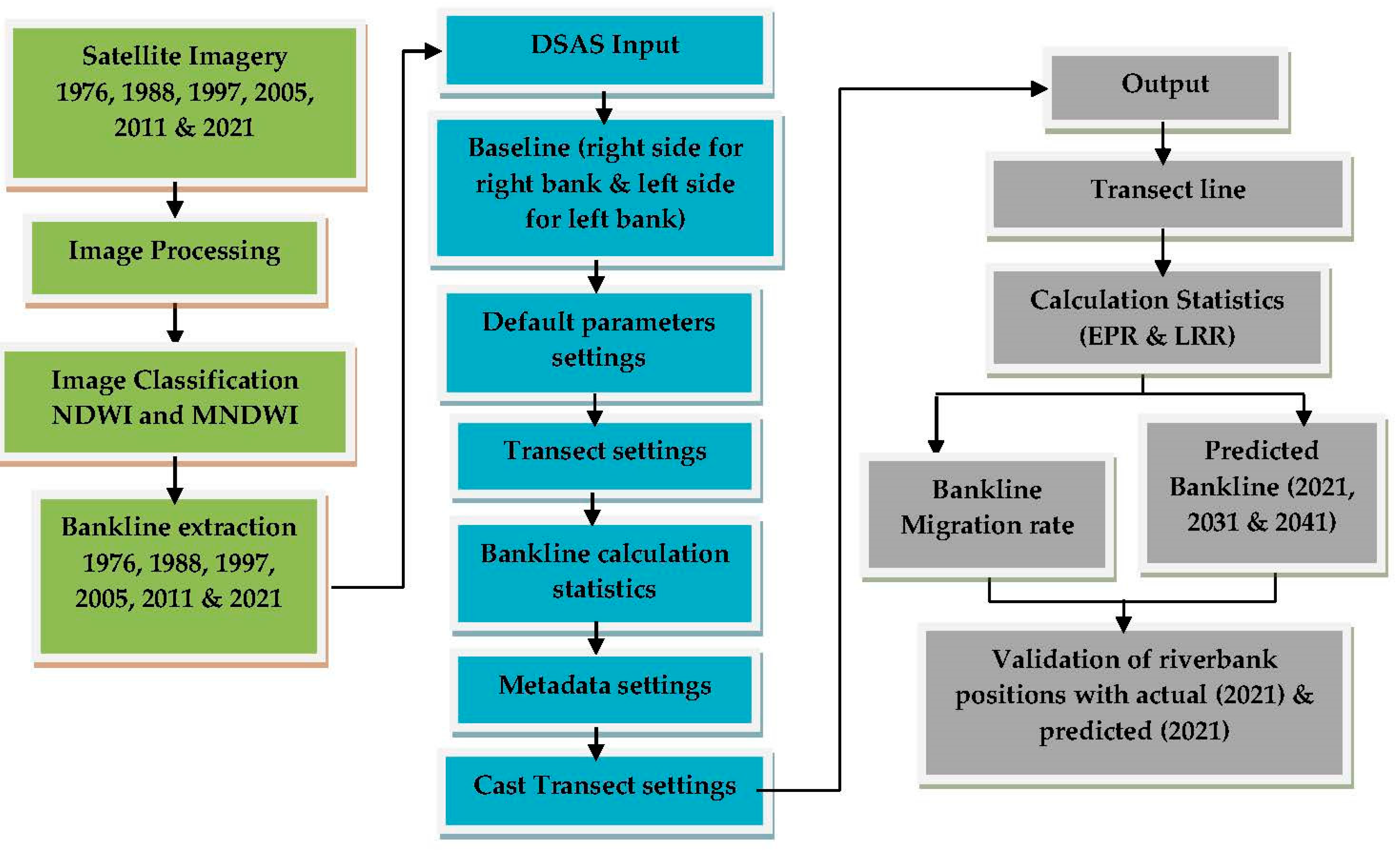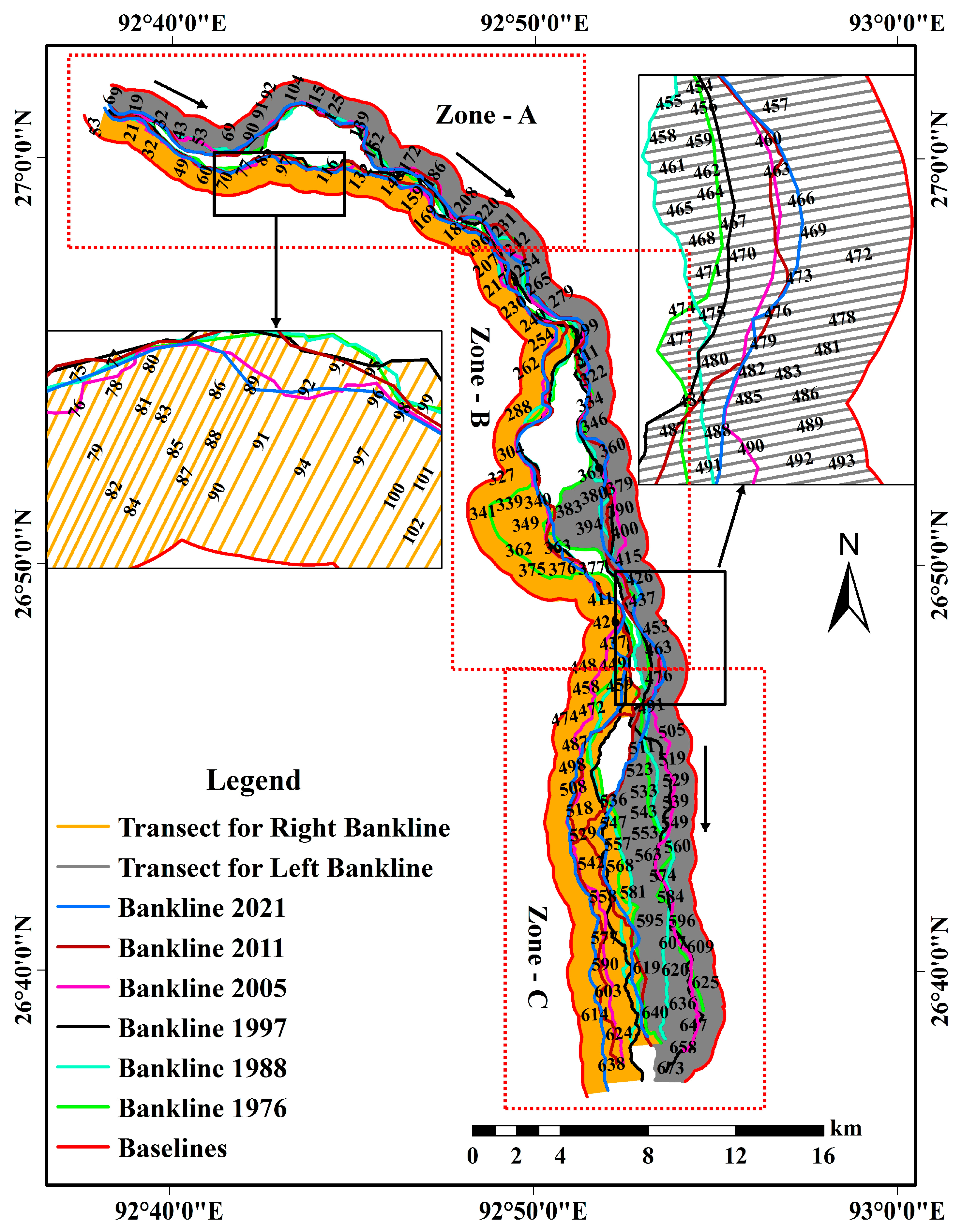Automated hybrid techniques recently developed to predict channel migration rates are being increasingly used [11,26]. The United States Geological Survey (USGS) created the Digital Shoreline Analysis System (DSAS), a widely used computerized method, that allows for calculating the rate of shoreline change from various coastline sites. It is a free tool and is compatible with the ArcGIS software. It compares shoreline/bankline positions over time to generate a variety of statistical change measures. The DSAS method is widely used to estimate channel shifting rates by discretely considering the right and left banks [11,27,28,29]. Usually applied to monitor sea shoreline changes, it is amenable to accurately measuring river bankline shifting as well [30,31]. This analysis was conducted in the Jia Bharali River of the Brahmaputra floodplain region in India. The river has experienced extensive erosion and deposition. The river has tremendous power to erode its banks due to its large discharge, fast flow velocity, especially during the monsoon season, and braided nature. The lower floodplain’s agricultural lands are severely harmed by bank erosion and floods. The river spreads its massive discharge and follows a meandering course downstream as it descends from the higher gradient of the Himalayan Mountain range onto the plain.

The Jia Bharali River is renowned for its exceptionally high flow during the rainy season, ongoing changes in channel morphology, rapid bed aggradation, and bankline modification, resulting in the lateral displacement of banklines and the annual collapse of extensive fertile land. Deb and Ferreira [14] argue that unless appropriate precautions are taken to mitigate this risk, the negative impacts of bank erosion and river movement on local livelihoods will continue to persist and worsen due to the impacts of climate change.

Climate change exacerbates this phenomenon of riverbank shifts [32], which can lead to more severe consequences, such as human casualties. One of the most significant impacts of climate change on river systems is altered precipitation patterns. In many regions of the world, climate change is expected to result in more frequent and intense rainfall events, which can increase the volume and velocity of water flowing in rivers. This can cause the more rapid and frequent erosion of riverbanks, leading to the lateral displacement of banklines and the collapse of large tracts of fertile land. Additionally, changes in temperature and precipitation can affect vegetation cover in river basins, altering the amount and type of vegetation along riverbanks. Vegetation plays a crucial role in stabilizing riverbanks by anchoring soil and slowing down the velocity of water flow. Changes in vegetation cover can therefore affect bank stability, making them more vulnerable to erosion and shifting.

However, in the present work, we have not considered the impact of climate change on the bankline shifts in the study area. The Jia Bharali River is known for its exceptionally high flow during the rainy season, ongoing changes in channel morphology, rapid bed aggradation, and bankline modification, resulting in the lateral displacement of banklines and the annual collapse of extensive fertile land. We used the DSAS model that considers past changes in bankline shifts and simulates future changes based on that information, regardless of the cause of past shifts and whether or not they were due to short-term climate change cycles, such as El-Nino or La-Nina. The model uses shift trend information to project future changes [27,28].

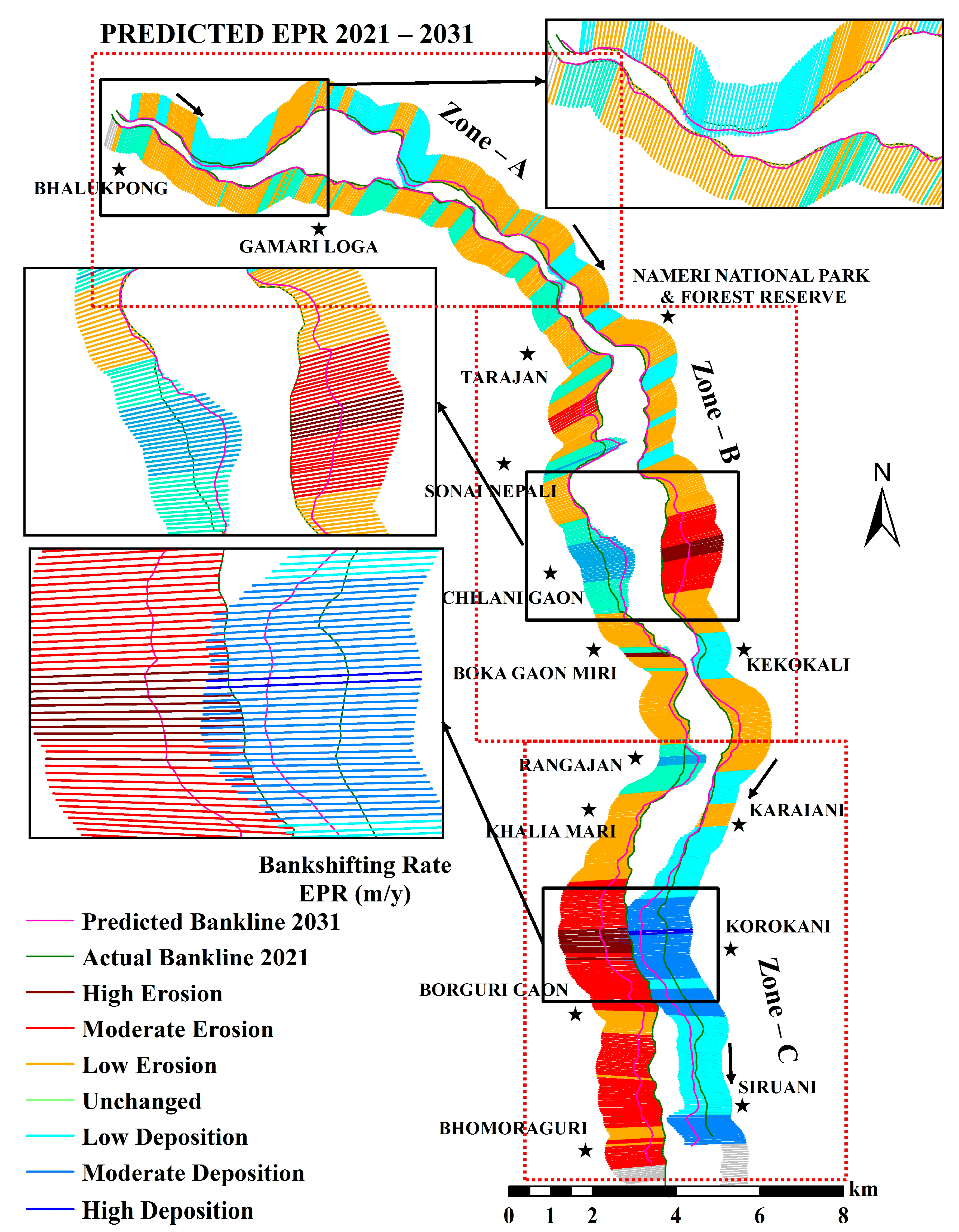
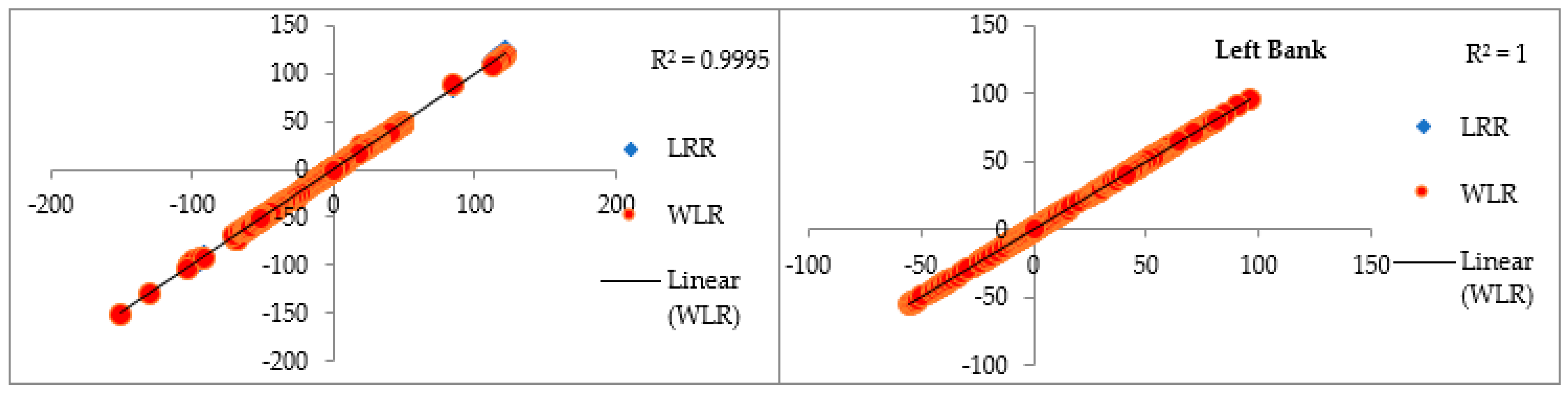
The lower section of the Jia Bharali River is prone to recurrent flooding and channel shifting, which has had a significant negative impact on the socioeconomic status of floodplain dwellers. However, little scientific work has been conducted on bankline changes in the river and previous studies have not estimated the rate of bank erosion or predicted future banklines. To address this gap, the present analysis uses a reference baseline and transects to estimate riverbank erosion rates using end point rate (EPR) and linear regression rate (LRR), as well as DSAS-based statistical models to project where the bankline will be in 2031 and 2041. The results of this research could prove to be helpful to policymakers seeking to develop strategies to alleviate the effects of bankline shifts on local economies and food security.

2. Study Area

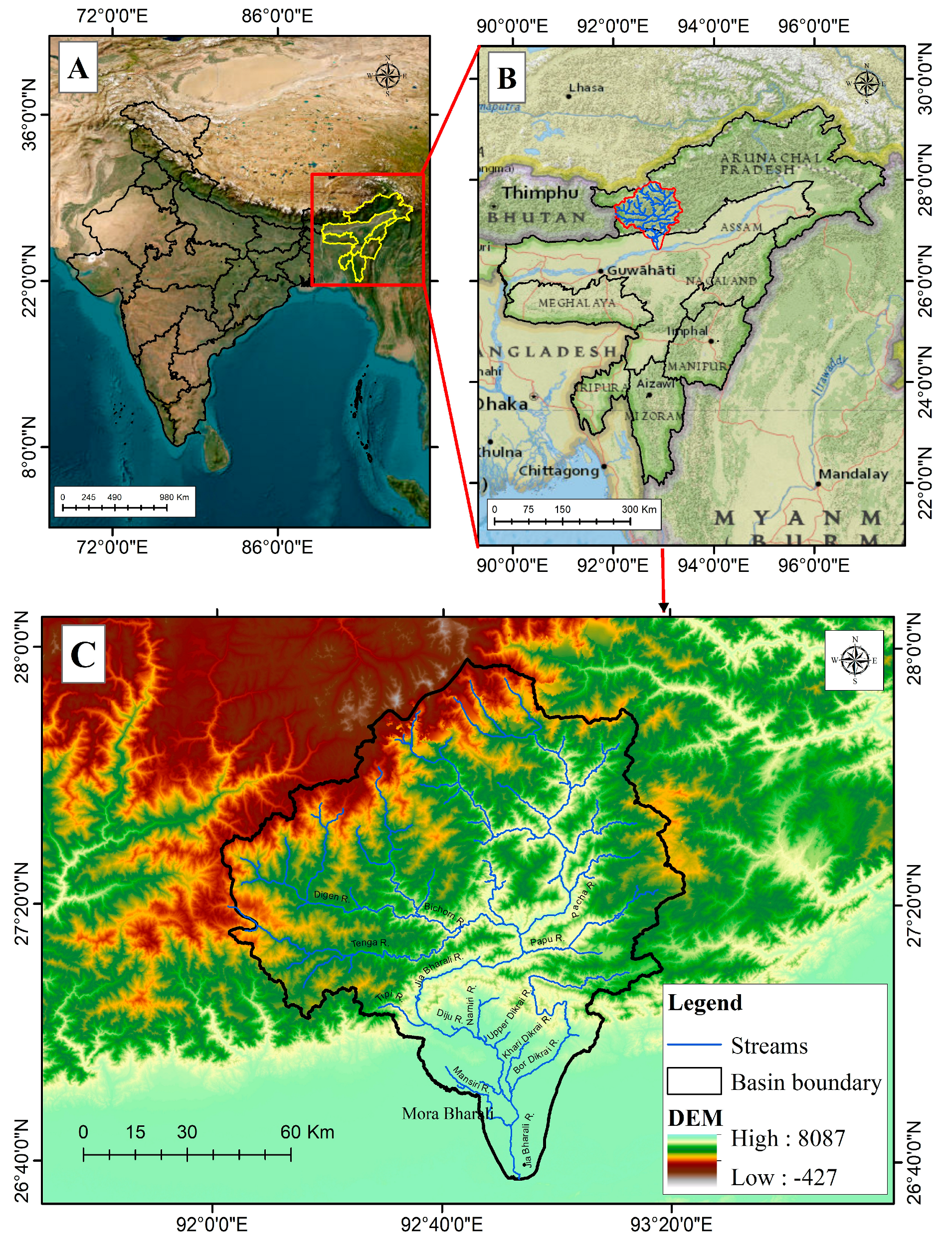
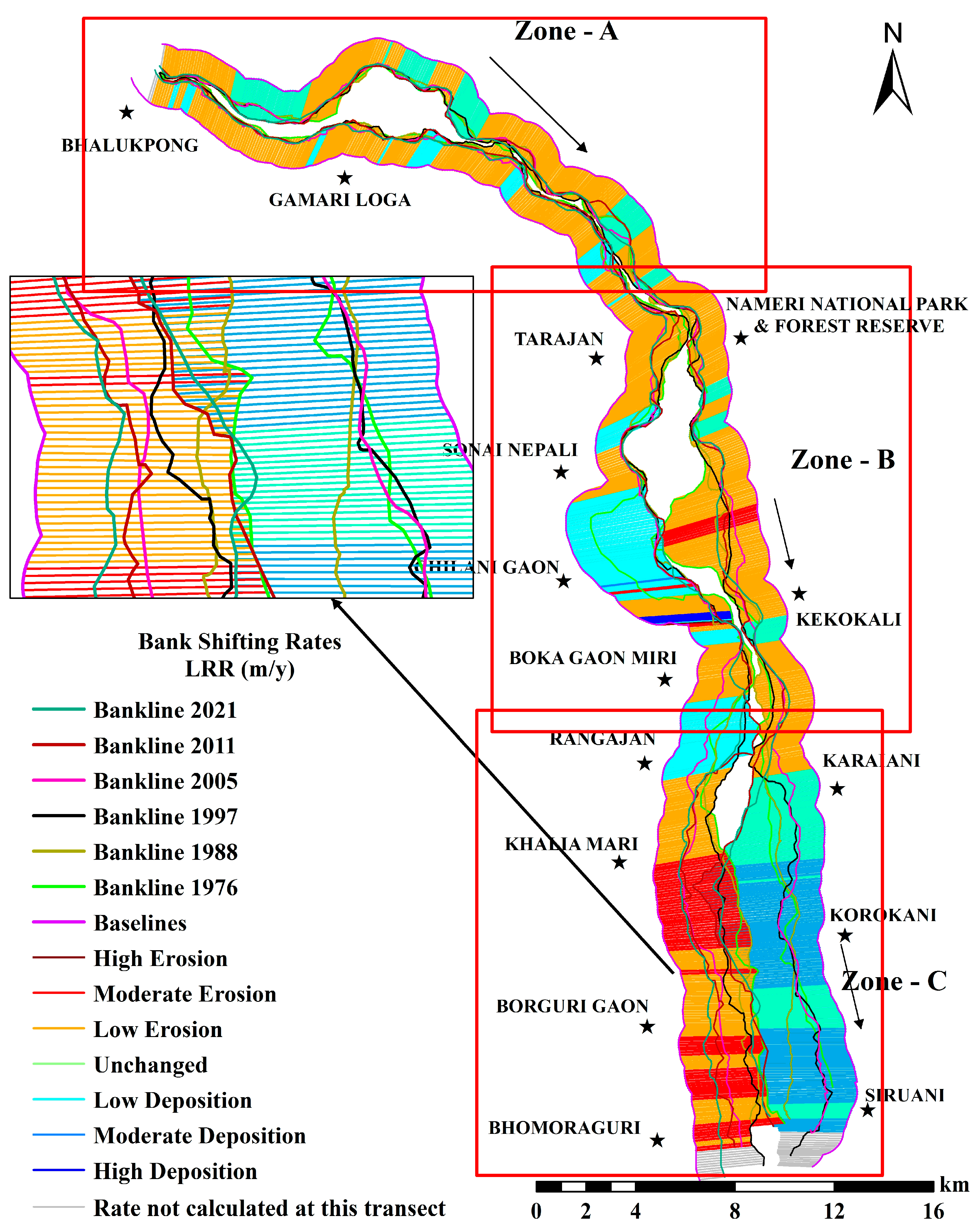
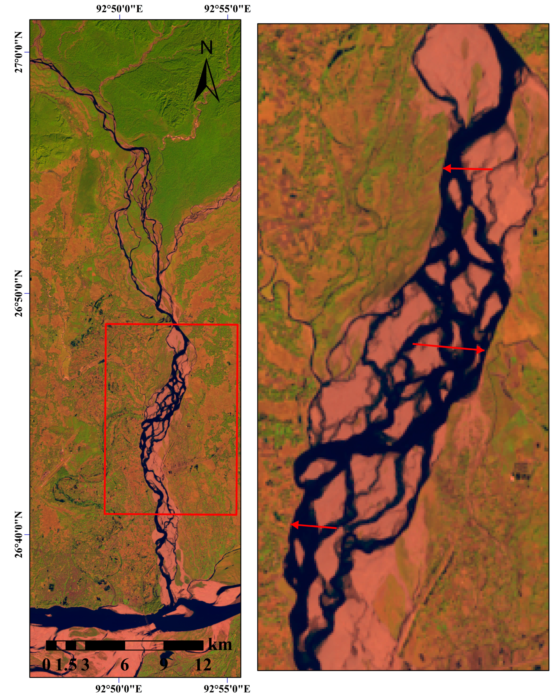
The Jia Bharali basin, located between 26°37′ N to 28°00′ N latitudes and 92°00′ E to 93°25′ E longitudes, covers an area of 11,716 km². The basin lies in the Indian provinces of Assam and Arunachal Pradesh and consists of 6.7% of the entire catchment area of the Brahmaputra River system. Of the total basin area, 10,239.8 km² (87.4 percent) lies in Arunachal Pradesh’s mountains, while 1476.6 km² (12.6 percent) is in Assam (Figure 1). The Great Himalayan Range provides the source of Jia Bharali, a north-bank tributary of the Brahmaputra River, which starts at 4520 m above sea level and flows 247 km through mountains, valleys, and plains before joining the Brahmaputra. The Bichom, Tipi, Nam Sonai, Dharikati, and Mansiri are its right bank tributaries, while Pacha, Papu, Diju, Namiri, Upper Dikrai, Khari Dikrai, and Bor Dikrai are its left bank tributaries. These are streams that originate from the Himalayan Mountain ranges.

The Jia Bharali is called Kameng at its 185 km stretch in Arunachal Pradesh. With three-fourths of its length across hilly terrain, the river carries a substantial amount of silt [33]. It begins losing velocity as it enters the Brahmaputra plains, getting progressively slower as it flows downstream. Here, the river becomes braided as most of the sediment is deposited on the riverbed. Additionally, because of the high velocity and enhanced erosive capacity, especially in the southwest monsoon, the river begins changing its course. The river significantly shifts the morphology of its channel through a complex interaction between braiding the channel during non-monsoon seasons due to decreasing sediment load carrying capacity and alters its route during monsoon in the lower course. The Brahmaputra floodplain is situated in one of the largest seismically active regions of the planet. The Brahmaputra and its tributaries are experiencing faster rates of bed aggravation and an increase in the threats of flooding and erosion, as fallout of the 1950 earthquake. Moreover, anthropogenic activities, such as building embankments along the river, deforestation in the upper catchment areas and unscientific gravel, and sand quarrying from the river bed have cumulatively had deleterious effects on the normal flow of the river. Our analysis focuses on the river’s lower course where erosion and deposition are at a peak (Figure 1).

3. Materials and Methods

3.1. Datasets Preparation

Landsat Multispectral Scanner System (MSS) 1976, Thematic Mapper (TM) 1988, and 1997, Enhanced Thematic Mapper Plus (ETM+) 2005 and 2011, and Operational Land Imager (OLI) 2021 were used (

Table 1. Details about the data sources used in the study.

Serial No.	Sensor	Path/Row	Acquisition Date	Spatial Resolution
1	MSS	146/41	16 November 1976	60
2	TM	136/41	11 January 1988	30
3	TM	136/41	19 January 1997	30
4	TM	136/41	01 January 2005	30
5	ETM+	136/41	23 January 2011	30
6	OLI	136/41	20 December 2021	30

). Post-monsoon season images were selected keeping cloud cover constraints in mind. The UTM projection, UTM zone 46 north, and the WGS84 datum were used to project the Landsat images. Pre-processing enhancements such as haze removal, sharpness, and contrast were performed. The images were mosaicked together to create a single image encompassing the whole extent of the river. The entire stretch had been split into 3 distinct zones, spanning a distance of 20 km to facilitate the analysis.

3.2. The Demarcation of Banklines, Baselines, and Transect

The mid-infrared (MIR) and shortwave-infrared (SWIR) wavelengths bands of Landsat 7, 5, and 8 respectively, are capable of distinguishing water and vegetation [11,26]. The lower course of the river’s land-water boundaries were marked using pixel-resampling and band-mathematical rationing procedures. The Normalized Difference Water Index (NDWI) and Modified Normalized Difference Index (MNDWI), (Equations (1) and (2)) were used to identify banklines.Water was represented by pixels with the value “1” and land was represented by pixels with the value “0”.

$$NDWI=\frac{Green-NIR}{Green+NIR}$$

(1)

The MNDWI calculation is as follows:

$$MNDWI=\frac{Green-MIR}{Green+MIR}$$

(2)

$$NDWI=\frac{Green-SWIR}{Green+SWIR}$$

(3)

To compare the rate of channel shifting, we divided the analysis into five sub-periods, namely 1976 to 1988, 1988 to 1997, 1997 to 2005, 2005 to 2011, and 2011 to 2021.The composite line was traced using the final line of overlapping visualization for the overlay bankline position for each dataset. The baselines for the right and left banks were then individually produced using a 1000-m buffer from the composite line. Subsequently, 650 transects had been created at 100-m intervals along the baseline for the entire selected section of the Jia Bharali River. These transects were created with a 5 m uncertainty at an acute angle to the baseline and up to 10 km from the banks.

3.3. Assessment of Bankline Shifting Rat

The EPR was estimated after dividing the distance of bankline migration by the amount of time between the oldest and most recent bankline. It was determined using the equation shown below:

$$EPR=\frac{Distance of bank line movement }{Time between oldest and most recent}$$

(4)

The DSAS model’s EPR method is based on the premise that the actual periodic change rate of bankline position provides the most accurate forecast for the future bankline position [34]. Since the position history captures the combined effects of the processes, this assumption negates the necessity for prior knowledge of flow discharge or sediment movement [35]. To predict the spatio-temporal change of the bankline and rate of river erosion-deposition [36], EPR was determined for the periods 1976 to 1988, 1988 to 1997, 1997 to 2005, 2005 to 2011, and 2011 to 2021.

Y was used for the earlier (Y_ob) and recent (Y_rb) banklinepositions. Y represents the expected bankline location and was calculated using Equation (5):

$$Y={\alpha }_{EPR}+{\beta }_{EPR }\mathrm{X}$$

(5)

where: ${\alpha }_{EPR}$ stands for the model intercept; ${\beta }_{EPR }$ for riverbank shifting rate [slope or regression coefficient]; X for the time gap (X_ob − X_rb) between the earlier (X_ob) and recent bankline (X_rb).

The EPR intercept is calculated using Equation (6).

$${\alpha }_{EPR}=Y_{ob}-\left\{\frac{Y_{ob}-Y_{rb}}{X_{rb}-X_{ob}}\right\}{X}_{ob}=Y_{rb}-\left\{\frac{Y_{ob}-Y_{rb}}{X_{rb}-X_{ob}}\right\}{X}_{rb}$$

(6)

The bankline change rate for particular sets of the transect [${\beta }_{EPR }$] is calculated using the Equation (7):

$${\beta }_{EPR}=\left\{\frac{Y_{ob}-Y_{rb}}{X_{rb}-X_{ob}}\right\}$$

(7)

3.4. Prediction of Bankline

The predictions for the next 10 and 20 years were computed using the previous bankline position data in the new DSAS version 5.0 [37]. The Long and Plant Kalman Filter [38], which merged the observed bankline locations with the model-derived locations, was typically used to estimate the future bankline position. Kalman Filters require a set of linear regression rates (LRR) to precisely forecast banklines. In order to represent the bank position for the following year of the chosen time period, the LRR model uses data of the model-generated baseline that are delineated by the temporal period of bankline migration for 1976 to 1988, 1988 to 1997, 1997 to 2005, 2005 to 2011, and 2011 to 2021. It follows that the baseline for all sets is the channel side location of dataset 2021. The least-squares method, which involves fitting a regression line to the results, has been used to forecast channel shifting [37]. Equation (8) is used to determine the bankline migration rate by fitting a regression line to each point along a particular user transect.

$$y=a+bx$$

(8)

where y is the dependent variable, whose value will be predicted or explained by x, a constant, and b is the slope of the regression line. The slope demonstrates how each unit of x influences how much y shifts.The rate is determined by the line’s slope in the equation defining it. The correlation coefficient (R²) was calculated to verify the association between the x and y values.

The DSAS moves through successive years, starting with the oldest bankline position, until it reaches the next bankline position. The Kalman Filter works to minimize observed discrepancies between the model and bankline position while interacting with a bankline position to carry out the forecast. The projected bankline for each succeeding position was calculated using the updated rate up until the date of the next test. Later, a new dataset was included in the model [37]. The process was repeated again until the desired forecast was attained.

Standard error and R² of the bankline change calculation: Calculating the bankline shifting involved estimating the rate of error for LRR and WLR data [39]. Equation (9) represents the anticipated baseline distance (y)of each bankline based on time (x):

$$y=mx+c$$

(9)

where m is the rate of change/slope; c is the y-intercept; y is the projected baseline distance.

After comparing the value of “y” to the known value on banking points, the accuracy is estimated by calculating the standard error of measurement. The Linear Standard Error and Weighed Linear Regression (WLR/WSE), which involves (LSE), was calculated (Equation (10)):

$$\mathrm{LSE} \mathrm{or} \mathrm{WSE} =\sqrt{\frac{\sum {\left[y-y^{\prime }\right]}^2}{n-2}}$$

(10)

where n is the number of banklines measured, y is the predicted value based on the best-fit regression line, and y′ is the length from the baseline to a particular bankline point.

The level of agreement is indicated by an R² score, with 1.0 representing the highest level and 0.0 the lowest. Linear regression rate (LR²) and weighted linear regression [WR²] are abbreviations used in the DSAS model. Equation (11) was used to define it:

$${\mathrm{R}}^2=1-\sqrt{\frac{\sum {\left[y-y^{\prime }\right]}^2}{\sum \left[y-\overline{y}\right]}}$$

(11)

where y stands for the distance from the baseline, y′ for projected distance from the baseline depending on the best-fit regression line, and y is the mean bankline distance from the baseline; R² is the coefficient of determination.

3.5. Validation of the Forecasted Bankline and Evaluation

Usually, the Shoreline Change Envelope (SCE) technique is used to confirm forecasted lines [39]. SCE was used in this analysis as a Bankline Change Envelope [BCE] to validate the projected bankline. Thus, banklines between 1976 and 2011 were processed using the DSAS to predict the bankline in 2021.The forecasted shoreline (2021) and actual shoreline (2021) retrieved from a Sentinel-2B satellite image (acquired in November-December 2021) were compared in a DSAS environment to measure differences between the actual and forecasted shorelines. The adopted methodology is shown in a flowchart (Figure 2).

4. Results

4.1. EPR-Based Periodic Riverbank-Shifting Trend

Three distinct zones, designated as A, B, and C, were divided up along the Jia Bharali River stretch. In each zone, about 215 transects (on both sides) were made to compute the rate of the bankline shift along with erosion and deposition (Figure 3). The erosion and deposition rate was graded according to its range; for example, a rate of erosion and deposition between 0 and 50 m/y was low, between 50.01 and 100 m/y was moderate, more than 100 m/y was high, and 0 m/y was unchanged (

Table 2. Erosion and Deposition Grade according to the range of the EPR/LRR rate.

Sl. no	Range of the EPR/LRR Rate	Remarks
1	0 to 50	Low Deposition
2	50.01 to 100	Moderate Deposition
3	>100	High Deposition
4	0	Unchanged
5	0 to −50	Low Erosion
6	−50 to −100	Moderate Erosion
7	>−100	High Erosion

).

During 1976 to 1988, the average shifting rate in the right and left banks of zone A, B, and C were −2.11 and 8.68 m/y, −34.72 and −34.96 m/y, and −12.24 and 12.17 m/y, respectively. On both banks, the average rate of erosion was −24.53 and −28.19 m/y and deposition was 59.71 and 28.27 m/y, respectively. During this period, the right bank experienced an average shifting of 7.28 m/y while the left experienced a shifting of −10.49 m/y (

Table 3. Right bank shifting rate of the Jia Bharali River using EPR approach of DSAS model.

Period	Zone	Average Rate of Erosion (m/y)			Average Rate of Deposition (m/y)			Average Rate of Shifting (m/y)
		High	Moderate	Low	High	Moderate	Low
1976 to 1988	A	0	0	−4.05	0	0	1.75	−2.11
	B	−376.81	−60.03	−9.82	241.29	81.32	4.73	34.72
	C	0	−74.2	−20.4	0	0	20.3	−12.24
	Total	−351.84	−66.28	−14.91	241.29	70.88	8.08	7.28
	Overall	−24.53			59.71
1988 to 1997	A	0	0	−5.23	14.06	69.92	0	6.1
	B	−441.39	0	−6.14	218.3	63.95	16.57	−1.06
	C	−112.8	−77.48	−17.24	110.28	71.79	26.45	−3.36
	Total	−178.21	−76.79	−8.48	134.39	69.9	16.69	0.52
	Overall	−25.27			35.99
1997 to 2005	A	0	−69.45	−13.78	0	0	2.44	−17.76
	B	−304.76	−61.69	−15.34	0	0	8.03	−42.61
	C	−155.19	−71.78	−30.13	0	0		−123.38
	Total	−171.41	−68.66	−15.14	0	0	7.47	−61.81
	Overall	−65.11			7.47
2005 to 2011	A	0	0	−4.88	0	61.27	14.8	14.79
	B	0	0	−7.93	173.83	66.49	16.83	21
	C	0	−69.29	−24.1	251.11	81.07	19.21	45.91
	Total	0	−69.29	−16.65	240.97	67.56	16.05	27.5
	Overall	−26.78			50.63
2011 to 2021	A	0	0	−9.62	0	0	3.29	−8.59
	B	−500	−65.23	−11.22	449.79	0	12.76	−1.97
	C	0	−66.71	−19.79	0	0	2.89	−26.57
	Total	−368.46	−65.68	−13.22	449.79	0	10.04	−12.42
	Overall	−20.42			27.63
1976 to 2021	A	0	0	−2.92	0	0	2.72	−2.21
	B	−117.97	−83.36	−8.91	136.01	58.06	20.78	3.83
	C	0	−55.76	−34.56	0	0	15.85	−29.09
	Total	−117.97	−61.02	−14.56	136.01	58.06	15.26	−9.22
	Overall	−19.71			28.06

and

Table 4. Left bank shifting rate of the Jia Bharali River using EPR approach of DSAS model.

Period	Zone	Average Rate of Erosion (m/y)			Average Rate of Deposition (m/y)			Average Rate of Shifting (m/y)
		High	Moderate	Low	High	Moderate	Low
1976 to 1988	A	0	−63.03	−8.3	0	0	3.27	−8.68
	B	−191.29	−61.91	13.23	0	0	9.74	−34.96
	C	0	0	−18.94	116.65	70.12	23.84	12.17
	Total	−191.39	−62.8	−12.97	116.65	70.12	12.29	−10.49
	Overall	−28.19			28.27
1988 to 1997	A	0	0	−7.67	0	0	11.83	4.07
	B	0	−59.52	−15.98	107.04	74.68	16.62	10.86
	C	−152.03	−70.39	−25.38		71.64	9.26	−41.85
	Total	−152.03	−68.6	−14.48	107.04	72.99	14.21	−9.04
	Overall	−44.35			26.53
1997 to 2005	A	0	−54.44	−10.57	0	66.18	10.99	−6.06
	B	0	−71.57	−19.28	0	0	0.87	−32.16
	C	−122.18	−59.81	−17.47	0	0	15.6	−21.25
	Total	−120.85	−65.86	−15.54	0	85.24	8.26	−19.85
	Overall	−26.87			18.59
2005 to 2011	A	0	0	−8.43	0	76.21	11.68	9.11
	B	−105.87	−76.17	−14.59	114.91	76.29	14.70	7.73
	C			−15.14	393.34	66.73	13.46	291.53
	Total	−105.87	−76.28	−11.54	383.33	75.35	12.93	103.51
	Overall	−20.19			159.97
2011 to 2021	A	0		−8.03	0	0	8.16	−2.53
	B	0	−57.23	−16.22	0	58.14	16.11	0.86
	C	0	−63.56	−19.48	0	58.83	13.97	−12.8
	Total	0	−61.28	−14.1	0	58.3	13	−4.92
	Overall	−18.29			16.94
1976 to 2021	A	0	0	4.94	0	0	6.22	−2.03
	B	0	−57.04	−12.27	0	0	5.33	−11.09
	C	0	0	−10.89	0	60.87	31.12	30.42
	Total	0	−57	−8.92	0	60.87	18.51	5.8
	Overall	−10.38			29.78

). While both erosion and deposition were equally active on the left bank, deposition was more active than erosion there (Figure 4 and Figure 5). However, the left bank had a negative [erosion] shifting while the right bank experienced a positive (deposition) shift in much of the river during 1976–1988. Zone B had the highest level of river dynamic activity (Figure 6).

From 1988 to 1997, the average erosion and deposition rates were −25.27 and −35.99 m/y and 35.99 and 26.53 m/y in the right and left banks, respectively. During this time, the right and left banks registered average shifts of 0.52 m/y and −9.04 m/y, respectively (Table 3 and Table 4), which were less than that during the previous period. Deposition was more active in the right bank, whereas erosion predominated in the left bank (Figure 4 and Figure 5). The average rate of shifting was negative in the left bank and positive in the right bank. Zone C had the highest level of dynamic activity, followed by zone B (Figure 6). Overall, in this period, both erosion and deposition rates were lower than that accruing during 1976–1988.

From 1997 to 2005, the average shifting rates in the right and left banks of zone A, B, and C were −17.76 and −6.06, −42.61 and −32.16, and−123.38 and −21.25 m/y, respectively. The average rates of deposition and erosion in the right and left banks were −65.11 and −26.87 m/y and 7.47 and 18.59 m/y, respectively. Right bank shifting averaged −61.81 m/y, whereas left bank shifting averaged −19.85 m/y over this time period (Table 3 and Table 4). Thus, erosion processes were more active during 1997 to 2005 at both banks (Figure 4 and Figure 5), with rates comparatively higher on the right bank.

River dynamicity was higher in zones B and C (Table 3 and Table 4). Thus, channel expansion, rather than narrowing, predominated at both banks. From 2005 to 2011, the average erosion rate was −26.78 and −20.19 m/y and deposition was 50.63 and 159.97 m/y at the right and left banks, respectively. The right bank experienced a lower average shifting of 27.5 m/y compared with the left bank (103.51 m/y) (Table 3 and Table 4). Thus, depositional processes were more dominant than erosion (Figure 4 and Figure 5), with higher deposition on the left bank. River dynamicity was highest in zone C. In this period, the rate of deposition was higher than in all previous periods. From 2011 to 2021, the average shifting rate in the right and left banks of zone A, B, and C were −8.59 and −2.53 m/y, −1.97 and 0.86 m/y, and −26.57 and −12.8 m/y, respectively. During this time, the right as well as left banks experienced an average shifting of −12.42 m/y and −4.92 m/y, respectively.

The results showed that both the right and left banks experienced erosion and deposition processes simultaneously (Figure 4 and Figure 5). Moreover, transect location shows that the right bank experienced greater erosion compared with the left bank and that river dynamicity was higher in zone C compared with other zones. The results highlighted that the negative (erosion) shifting rate was more prevalent on both banks compared with the preceding period. Channel expansion predominated during the time period of 2011 to 2021.

During 1976 to 2021, the average shifting rate in the right and left banks of zone A, B, and C were −2.21 and −2.03, 3.83 and −11.09, and −29.09 and 30.42 m/y, respectively. The right bank had an average shifting of −9.22 m/y whereas the left bank recorded a shifting of 5.8 m/y. Erosion was more active in the right bank, while deposition occurred at both banks. In the right bank, the average shift rate was negative (erosion), but in the left bank, it was positive (deposition). The level of erosion (right bank) and deposition (left bank) was greatest in zone C, whereas dynamicity was lowest in zone A. Channel expansion predominated over narrowing stemming from greater erosion rather than deposition.

4.2. LRR-based Shifting/Erosion and Deposition Rate

The LRR-based migration/erosion and deposition rates during 1976 to 2021 (Figure 5) resemble EPR trends (Figure 6). On both banks, the average erosion rate was −20.96 and −10.61 m/y and deposition was 22.20 and 31.23 m/y, respectively. Right bank shifting averaged −10.78 m/y, whereas left bank shifting averaged 6.7 m/y over this period (

Table 5. Bank shifting rate of the Jia Bharali River using LRR approach of DSAS model.

Zone	Grade	Average Rate of Erosion (m/y)		Average Rate of Deposition (m/y)		Overall Shifting
		Right Bank	Left Bank	Right Bank	Left Bank	Right Bank	Left Bank
A	High	0	0	0	0	−2.03	−1.52
	Moderate	0	0	0	0
	Low	−3.13	−5.31	2.9	6.65
B	High	−121.44	0	116.88	0	0.21	−10.51
	Moderate	−74.44	−53.31	85.1	0
	Low	−9.79	−12.8	26.24	3.8
C	High	0	0	0	0	−30.35	32.01
	Moderate	−55.89	0	0	62.4
	Low	−32.79	−13.41	17.35	34.71
Overall		−20.96	−10.61	22.2	31.23	−10.78	6.7

). The average shift rate was negative and positive (deposition) on the right and left banks, respectively. The dynamicity was higher in zones C and B relative to zone A. Channel expansion, rather than narrowing, predominated throughout the 46 year study period.

4.3. Prediction of Bankline Shift Using the DSAS Model

The future bankline of the Jia Bharali River was predicted for 2021 and 2031 using the DSAS model (Figure 7). The predicted results show that the average rate of bank migration in zones A, B, and C would be −0.61 and −0.55 m/y, −0.86 and −17.88 m/y, and −42.5 and 23.42 m/y in the right and left banks over 2021 to 2031, respectively. The predicted results show that during the period from 2021 to 2031, zone A would experience less erosion and deposition processes, zone B would experience moderate rates of erosion and deposition processes, and zone C would experience high grades of erosion and deposition processes, comparatively (Figure 8). During 2021 to 2031, channel expansions would predominate over the channel narrowing due to a higher negative (erosion) shift compared with a positive (deposition) shifting rate. Moreover, the right bank of zone C would be more vulnerable to bank erosion.

During 2021 to 2041, the average channel shifting rate in zone A would be −1.52 and −0.16 m/y, zone B would be−1.68 and −13.52 m/y, and zone C would be −38.39 and 28.86 m/y in the right and left bank during 2021 to 2031, respectively. Over this time, the right bank would experience an average shifting of −13.9 m/y and the left bank would experience a shifting of 5.14 m/y (

Table 6. Predicted bank shifting rate according to EPR for the periods of 2021 to 2031 and 2021 to 2041.

Period	Zone	Grade	Average Rate of Erosion (m/y)		Average Rate of Deposition (m/y)		Overall Shifting
			Right Bank	Left Bank	Right Bank	Left Bank	Right Bank	Left Bank
2021 to 2031	A	High	0	0	0	0	−0.61	−0.55
		Moderate	0	0	0	0
		Low	−4.06	−10.66	5.71	10.39
	B	High	−87.5	−104.63	0	0	−0.86	−17.88
		Moderate	−58.83	−77.66	69.68	0
		Low	−10.61	−12.18	18.18	8.38
	C	High	−103.13	0	0	100.18	−42.5	23.42
		Moderate	−70.54	0	52	70.12
		Low	−29.58	−19.2	32.2	19.83
	Overall		−29.09	−20.39	21.12	24.34	−14.59	1.7
2021 to 2041	A	High	0	0	0	0	−1.52	−0.16
		Moderate	0	0	0	0
		Low	−3.38	−7.49	3.94	9.21
	B	High	−176.66	0	0	0	−1.68	−13.52
		Moderate	53.05	−61.66	56.26	0
		Low	−10.07	−12.59	19.87	5.58
	C	High	0	0	0	0	−38.39	28.86
		Moderate	−65.6	0	0	70.06
		Low	−29.95	−18.73	23.32	25
	Overall		−24.5	−14.87	17.64	27.34	−13.9	5.14

). The predicted result shows that during the period of 2021 to 2041, zone C would be highly susceptible to erosion and deposition processes compared with zone A and B. Transect location shows that the maximum length of the right bank of zone C would experience moderate to low grades of the erosion process, whereas the maximum length of the left bank would experience a moderate to low grade of the deposition process. In zone B, both erosion and deposition processes with moderate to low grades are common but are less common than in zone C. In the A zone, the entire length of both the banks would experience low rates of erosion and deposition (Figure 9).

As in the period of 2021 to 2031, the period of 2021–2041 would also have the right bank of zone C being more vulnerable to erosion. During both periods, the right bank would be severely eroded, whereas the right bank would most likely experience high deposition. This long-term predicted result also shows that channel expansion will predominate over channel narrowing due to a higher negative (erosion) shifting rate compared with a positive (deposition) shifting rate. Nevertheless, due to the diversity of the various factors of bank erosion and accretion processes, such lateral migration could become sporadic as well as widespread in the future. The projected banklines often show that sediment deposition would occur along the left bank and that the bulkier expansion accrues along the right bank.

4.4. Standard Error Graph and R² Evaluation

The standard error graph and R² were estimated for accuracy assessment of the bankline change calculation using transects [39].The outcome demonstrates that, in both the right and left bankline change calculations, accuracy is high and the uncertainty is quite low in the WLR approach compared with the LRR method (Figure 10).According to these results, the WLR method is more precise than the LRR method [39,40]. The R² value in the computations for the right bank and left bank changes is one, indicating that the outcome is satisfactory (Figure 11).

4.5. Validation of the Forecasted Bankline and Evaluation

Figure 12 displays the BCE determined for the predicted and initial banklines. Red transects indicate a BCE rate greater than 10 m, yellow transects indicate a BCE rate less than or equal to 10 m, and green transects indicate a BCE rate less than 1 m. Generally, to evaluate the beta forecasting method’s precision, the BCE rate was determined using a 10 m default uncertainty buffer [37].

The BCE rate was calculated for a total of 632 and 677 transect locations in the right and left banklines, respectively. In 275 transect locations of the right bank, the BCE value was recorded between 0 and 1.0 m. In 204 locations, the value ranged between 1.0 and 10.0 m. Similarly, in 318 transect locations of the left bank, the BCE value was recorded between 0 and 1.0 m., and in 190 locations, a change between 1.0 and 10.0 m was recorded. This indicates that the bankline positions of the actual and the predicted bankline in 2021 remained the same in 76 percent of cases (479 transects) of the right bank and 75 percent (508 transects) of cases of the left bank. However, the difference in bankline positions between the two banklines was greater than 10 m in 24.21 percent of cases (153 transects) of the right bank and 24.96 percent of cases (169 transect) of the left bank (

Table 7. BCE for the validation of the predicted banklines.

Sl. no	Bankline Change Envelope (Range)	No. of Transects		Percentage Transects		Remarks
		Right Bank	Left Bank	Right Bank	Left Bank
1	0 to 1.0	275	318	43.51	46.97	Negligible variation
2	1.0 to 10.0	204	190	32.28	28.06	Variation within 10 m uncertainty band buffer
3	>10.0	153	169	24.21	24.96	Higher variation

). The projection appears to be significantly more deflective than the actual position in some areas. However, in more than 75 percent of cases, the bankline’s position and shape generally remain the same as the actual bankline. A field study was conducted to verify the erosion-prone areas shown in the prediction map.

5. Discussion

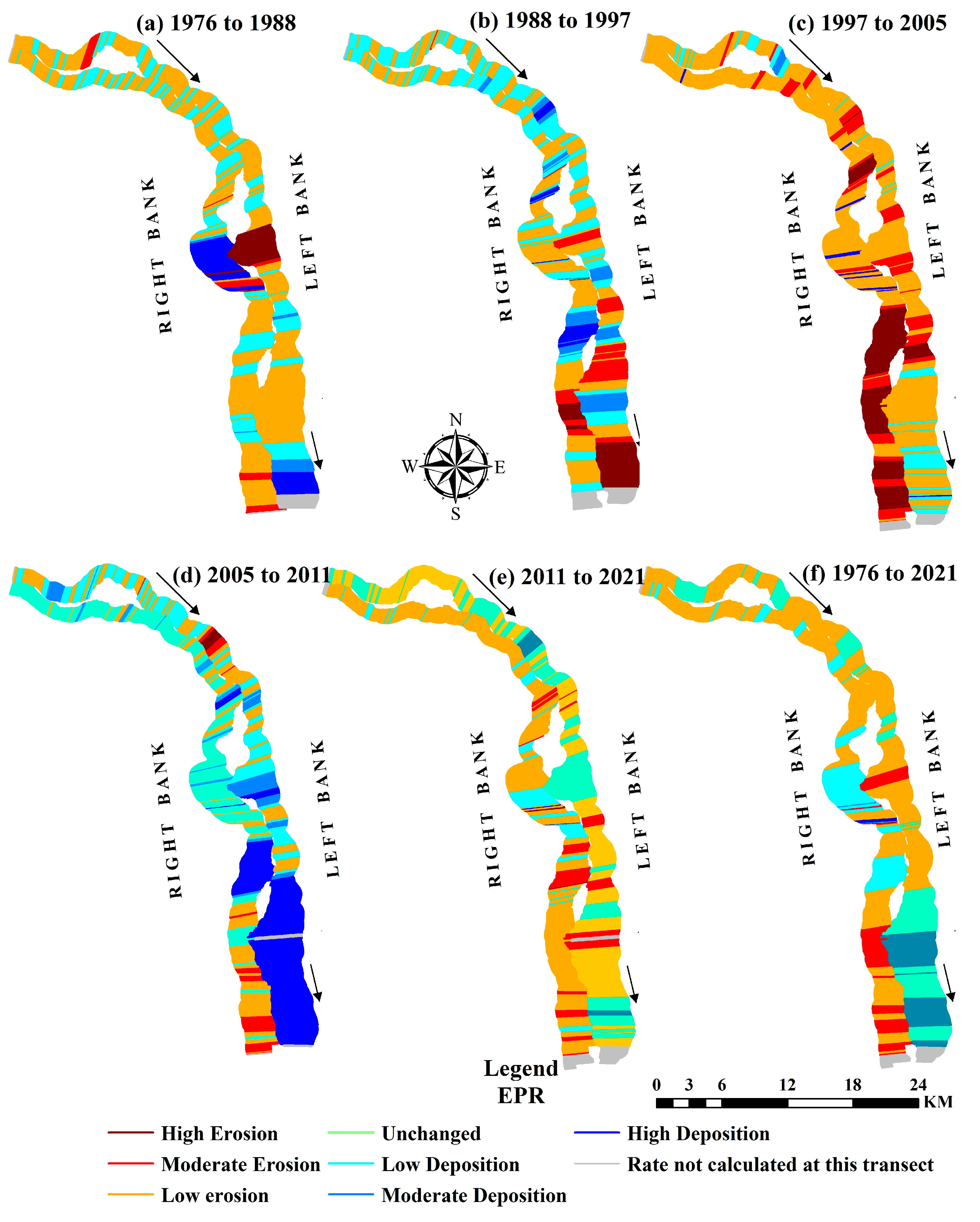
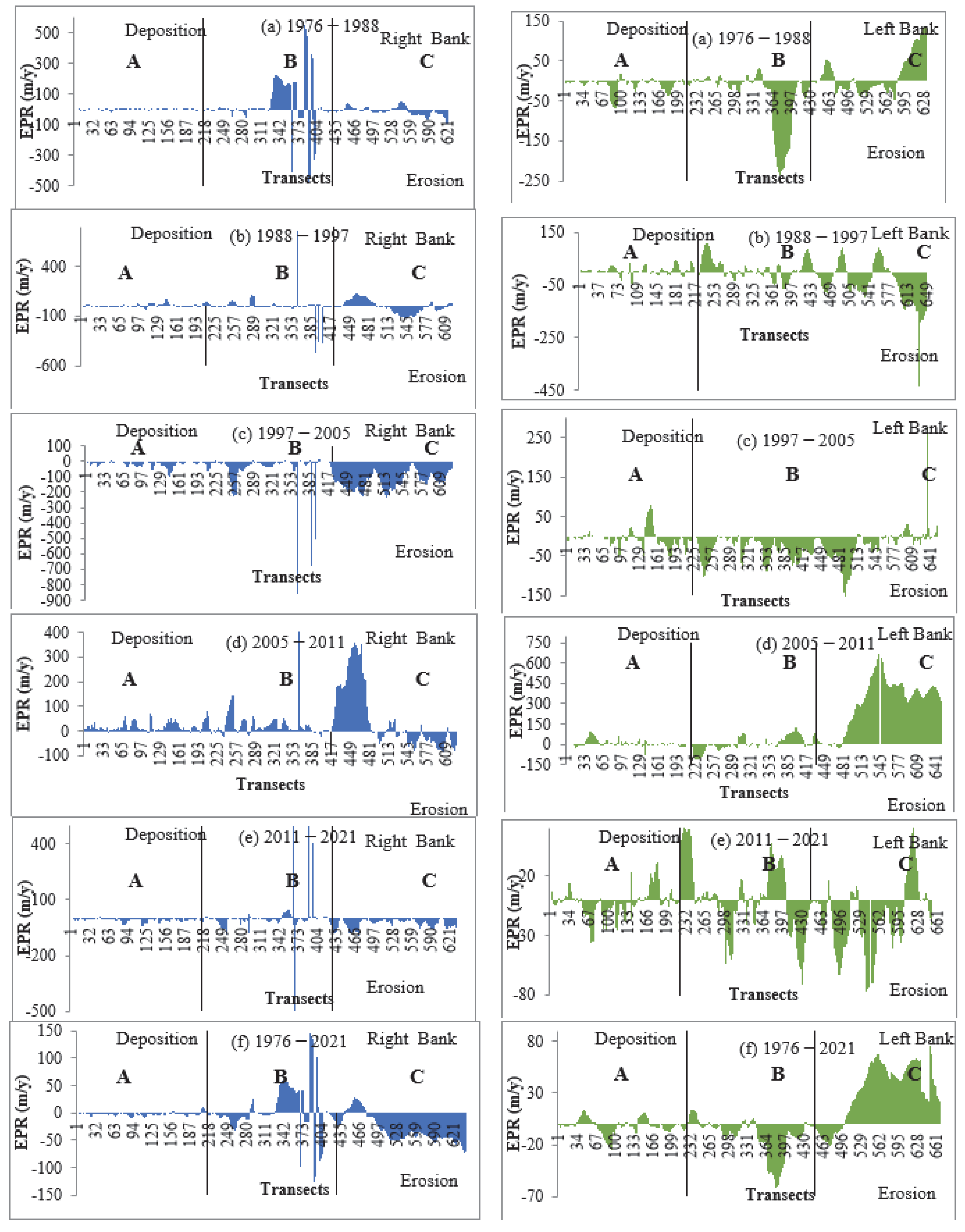
The Jia Bharali River underwent varying degrees of erosion and deposition from 1976 to 2021. Different periods were used to assess the erosion and deposition processes on its banks. Throughout the period, zones C and B had a high intensity of erosion as well as deposition. Significant bank erosion and deposition activities alongside river channel dynamicity occurred between1976–1988, 1988–1997, and 1997–2005, possibly on account of the intense and regular seasonal flooding episodes. During these periods, high and moderate erosion and deposition occurred in all zones of the river. The areas located immediately downstream of the confluence, especially the Bor Dikrai-Jia Bharali River confluence, experienced a high rate of erosion and deposition as well as significant lateral migration. A significant bank shift was observed in areas such as Bhomoragiri, Borgurigaon, Khaliamari, Karaiani, and Kekokali. Channel widening occurred in these areas because of ongoing and overturning erosion. However, the erosion process considerably slowed during 2005–2011, owing to the occurrence of low-magnitude floods in this region. However, due to an increase in the frequency of river flooding from 2011 onwards, the severity of high erosion and accretion increased once more in several locations during 2011–2021.

Both natural and man-made activities had an impact on the Jia Bharali’s migration. Rivers shift due to several reasons [4,41,42,43], including its braided character, minor and large floods, water discharge into the channel, bed load, bank material, terrain, tectonic activity, river confluence, thalweg shift, river flow direction, human involvement, etc. The flow pattern of the Jia Bharali River is altered by a mid-channel bar that is progressively growing, which affects the rates of channel migration, erosion, and deposition on both banks. Additionally, the river’s Assam part receives significant discharges from several tributaries that join it in this region, including the Bor Dikrai, Namiri, Diju, Upar Dikrai, Mansiri, Sonai, Nam Sonai, etc. The braiding processes of the Jia Bharali River have been greatly enhanced by increased water discharge and abrupt gradient changes. Several channel bars, both large and small, are created when the river channel is split into different segments. As a result, the cross-sectional area of the channel shrinks, forcing the river to move laterally in search of space. The research area is often found in an area with high rainfall, which increases the amount of water and debris that is discharged into the river, especially during the monsoon season. The river’s channel bed has been raised due to excessive sedimentation, which has reduced the channel’s ability to hold water. The river exerts pressure on the bank during the rainy season so that it can hold the extra water released. As a result, the riverbank erodes and the channel widens. Additionally, the extensive and frequent seasonal floods in the Jia Bharali River are significantly influenced by bed-level rise [33]. The Brahmaputra floodplain experienced severe flooding in the years 1954, 1962, 1972, 1973, 1977, 1978, 1983, 1984, 1987, 1988, 1991, 1993, 1995, 1996, 1998, 2004, 2016, 2017 [41], and 2022 [44]. The Brahmaputra valley was most affected by the 1998 flood [25,45,46]. Massive bank erosion typically happens during the floods’ receding stage, when too much sediment is deposited as sand bars in the channel, changing the flow direction and causing the sand bars to move there. It can also happen when the silt deposits on the banks fail to flow, which causes flowage [22]. The Jia Bharali’s banks are typically constructed of silt or sandy loam on the top layer and silt clayey or clayey loams in the deeper layers. These substances are easily eroded [47,48,49,50]. As a result, bank erosion is very frequent in this river [25]. Moreover, confluence zones of tributaries play an important role in bank erosion and lateral migration [5]. Channel geometry is altered by severe bank slumping, which triggers channel migration. One of the most frequent causes of bankline migration in the Jia Bharali River is the bowl-shaped shear failure induced by the removal of the basal support of blocks by erosion [33]. According to ground investigations, the left bank is experiencing a greater degree of bank slumping than the right. The channel in zone B moved eastward through bank slumping, which appears to be a frequent occurrence. In addition to altering bed configuration, the location of mid-channel bars has a considerable impact on the flow pattern of the river. The driving water increases the pore pressure in the channel wall when the thalweg approaches the bank after being deflected by several sandbars (Figure 13).

As a result, during receding flows, sand and silt move laterally into the river, causing subaqueous bank failure. Concave bends along the bankline eventually result from this. The Jia Bharali River runs through a region where the 1950 earthquake had a considerable impact. It seems reasonable to surmise that the tectonic event had a substantial impact on the current shape and behavior of the river, including its banklines. From the foregoing analysis, it appears that many parts of the Jia Bharali River, which are intensive subsistence agriculture, are at risk of flooding and bank erosion. As a result, embankments were built along the river for flood control. River channel morphology and flow dynamics are typically impacted by embankments along the river. Instead of positive outcomes, artificial embankments tend to exert extra strain on riverbanks [7]. This is a major factor in morphological changes, including the erosion of the riverbank and deposition on the floodplain. However, poor landuse practices in the floodplain near the banks and human-caused deforestation in the bank and upper catchment areas may have slightly contributed to bank erosion and slumping. The rapid change in banklines is accelerated by the unscientific exploitation of river sand and gravel, which also caused the banks to collapse in some sections. However, during the dry season, birds can be seen digging many holes in the exposed faces of sandy banks. As a result, such banks may fail more quickly during the monsoon, when rising river levels put a lot of hydraulic pressure on the bank wall and reduce the shear strength of the materials used to build the banks. Another significant human intervention made to improve erosion and deposition in the Jia Bharali River is the construction of bridges. The river has braided upstream and downstream of the rail and road bridges due to the hydrological constraints at the site. The stretch upstream of the rail and road bridges is braided because of the ponding [influx] effect caused by the narrow abutments of the bridges downstream, and as a result, some mid-channel bars have begun to form [51,52,53,54]. The lower stretch immediately downstream of the bridge site is braided because of the sediments that were deposited by the scouring at the site of the narrow bridge. As a result, bank erosion has significantly increased both upstream and downstream of the bridge locations. The Jia Bharali River has sensitive zones, and it is essential to evaluate riverbank erosion-deposition, as well as lateral channel migration, for planners, environmentalists, and policymakers to comprehend and develop sufficient channel design plans for those zones. In the present study, we have identified eroded and deposited parts of the Jia Bharali River from 1976 to 2021. Our suggestion to policymakers is to use a cadastral map along with our findings in this paper. This will help them to identify the actual landlord who has lost their land due to erosion and distribute the deposited land of the opposite bank to the victims. Moreover, the findings of the forecast can be used for the site selection of bank protection in order to protect the adjacent agricultural land and settlement.

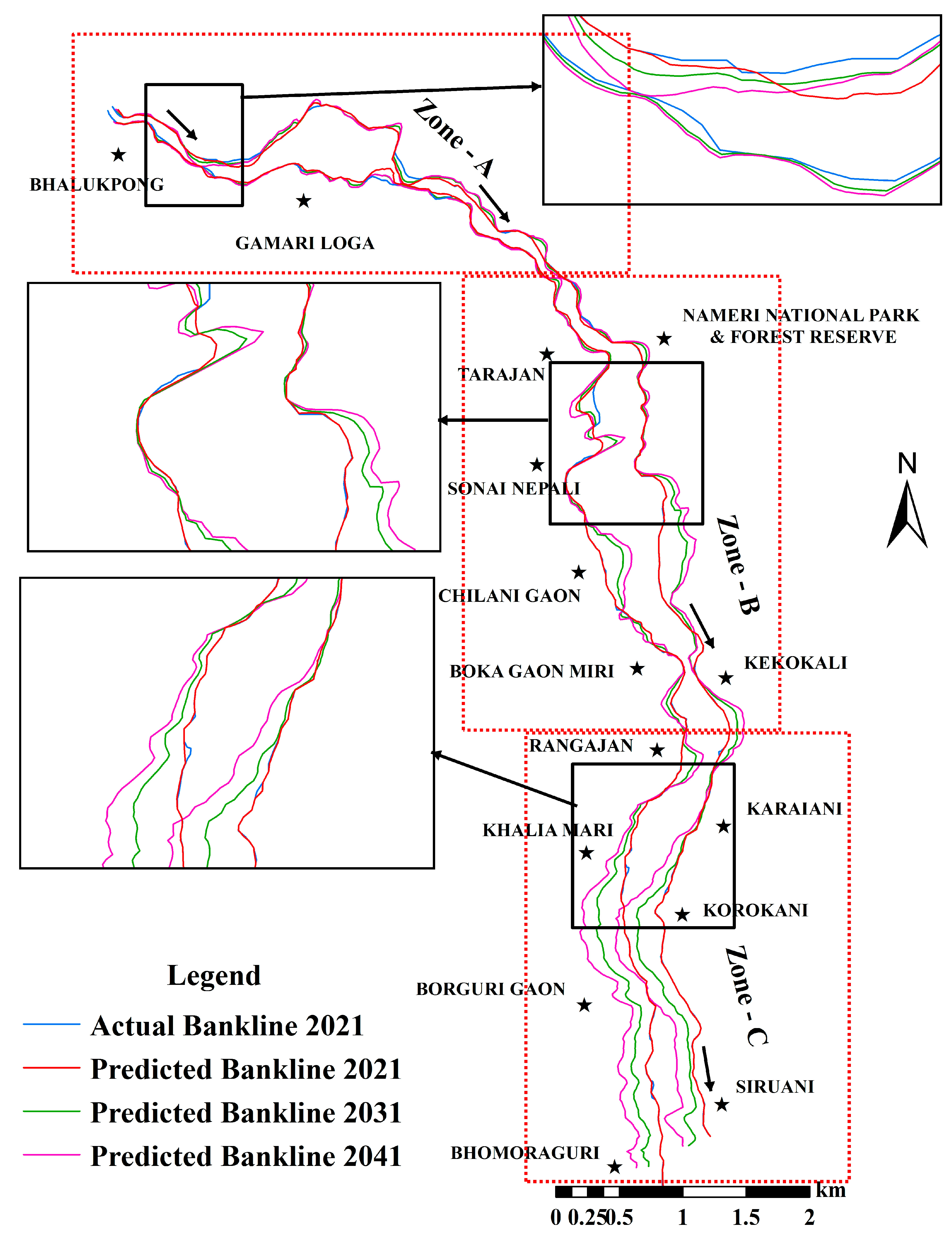
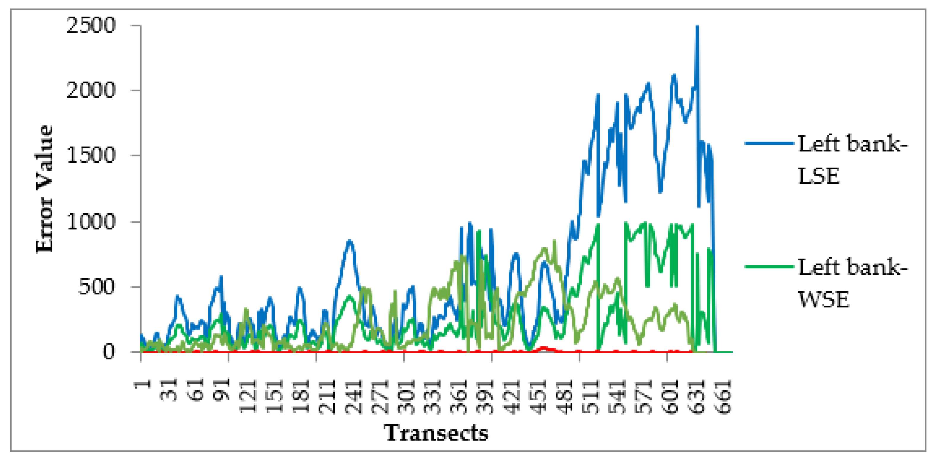
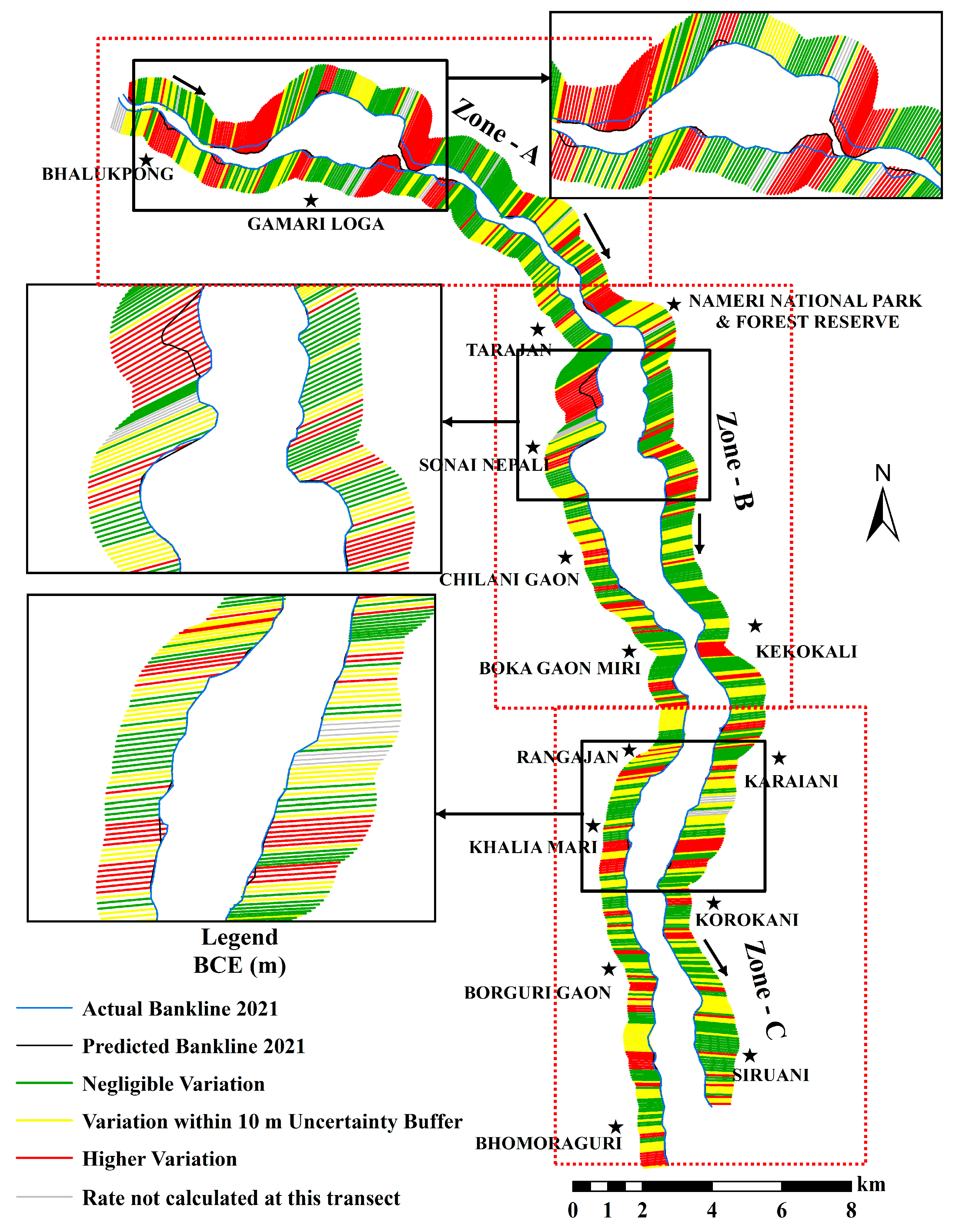
As compared with the previous version, the DSAS 5.1 tool is now capable of producing statistical data for more than 95% of the bankline used for the study. To enhance understanding of the dynamics of the shoreline/bankline, various DSAS model versions are being used. The application of predicting the future shoreline is a huge benefit to the research community as compared with earlier versions of this DSAS tool. The beta forecasting features use baseline data and historical trends to anticipate future shoreline position progress. The DSAS forecasting method will not be optimal for all locations, data types, and patterns of bankline change, as shown by the accuracy assessment of the projected bankline in the present study (Table 7 and Figure 12). However, while utilizing this program to ascertain a predicted bankline position, it has several limitations and restrictions on their data. As it is not possible to alter the DSAS forecasting tool, we should estimate future trends in a later stage of model development by taking into consideration all the influence factors. According to our opinion, the user is responsible for taking into account the details and constraints of their data while using this tool to predict future bankline position.

In the current study, we assessed the Jia Bharali River’s rate of bankline erosion and predicted future changes to the river’s bankline. The potential impact of extreme weather on soil erosion at the study site must also be taken into consideration in future studies [55,56,57,58]. In many parts of the world, climate change is predicted to lead to more frequent and intense rainfall events, which can increase the amount and speed of water flowing through rivers [59,60]. As a result, riverbanks may erode more quickly and frequently, causing lateral bankline displacement and the collapse of significant areas of fertile land [48,61]. Flash floods can be brought on by periods of heavy rain, which can cause significant soil erosion and sediment deposition. Climate change is predicted to result in an increase in the frequency and size of extreme rainfall events, which could accelerate soil erosion in the study area [62,63]. Additionally, because they reduce vegetation cover and expose more soil to wind and water erosion, extreme weather conditions like droughts and heat waves can also have an impact on soil erosion [64,65]. Reduced soil moisture levels during droughts can make soil particles more vulnerable to wind and water erosion. By securing soil and reducing water flow velocity, vegetation cover is essential for stabilizing river banks [66,67]. Therefore, changes in vegetation due to severe weather can have an impact on bank stability and make them more susceptible to erosion and shifting. The potential effects of extreme weather on soil erosion and bankline shifts in the study area must therefore be taken into account. To better understand the potential effects of climate change on the stability of riverbanks in the Jia Bharali River basin, future research should quantify the relationship between extreme weather events and soil erosion rates.

6. Conclusions

The current study evaluated geographical and temporal changes in the Jia Bharali River’s course with channel dynamicity using a geospatial model. The multi-temporal data analyses reveal that the river’s banklines were continuously altered by erosion and deposition. The river’s erosion and accretion rates were higher in early times than they have been in more recent times. Zones C and B are more adversely affected than zone A. Since the left bank of zone B experiences more erosion than the right bank, this zone is where the river is migrating to the left (eastward). Since the right bank of zone C is degrading more quickly than the left, this indicates that the river is flowing to the right (westward) in this zone. The anticipated outcome also shows that the right bank of zone C and the left bank of zone B will have greater average migration rates. Therefore, it was predicted that zone B’s left bank and zone C’s right bank would be most vulnerable to bank erosion. The current study estimated historical and future bankline movement using an artificial computing environment. Considerable ground verification and continuing observation are necessary for such automated systems. As a result, the automated DSAS-based methodology was adopted in the current analysis. This methodology can accurately measure and predict erosion and deposition. The projected and actual banklines were also used to compare the degree of accuracy. Future strategies, such as afforestation measures and limiting human interference to allow rivers to flow naturally and enhance the ecological and biological diversity of the floodplain zone [22,55], are necessary.

References

1. Rajib, A.; Zheng, Q.; Golden, H.E.; Wu, Q.; Lane, C.R.; Christensen, J.R.; Morrison, R.R.; Annis, A.; Nardi, F. The changing face of floodplains in the Mississippi River Basin detected by a 60-year land use change dataset. Sci. Data 2021, 8, 271. [Google Scholar] [CrossRef]
2. Costanza, R.; De Groot, R.; Sutton, P.; Van der Ploeg, S.; Anderson, S.J.; Kubiszewski, I.; Farber, S.; Turner, R.K. Changes in the global value of ecosystem services. Glob. Environ. Chang. 2014, 26, 152–158. [Google Scholar] [CrossRef]
3. Debnath, J.; Sahariah, D.; Lahon, D.; Nath, N.; Chand, K.; Meraj, G.; Farooq, M.; Kumar, P.; Kanga, S.; Singh, S.K. Geospatial modeling to assess the past and future land use-land cover changes in the Brahmaputra Valley, NE India, for sustainable land resource management. Environ. Sci. Pollut. Res. 2022. [Google Scholar] [CrossRef]
4. Debnath, J.; Das(Pan), N.; Ahmed, I.; Bhowmik, M. Channel migration and its impact on land use/land cover using RS and GIS: A study on Khowai River of Tripura, North-East India. Egypt. J. Remote Sens. Space Sci. 2017, 20, 197–210. [Google Scholar] [CrossRef]
5. Debnath, J.; Das(Pan), N.; Sharma, R.; Ahmed, I. Impact of confluence on hydrological and morphological characters of the trunk stream: A study on the Manu River of North-east India. Environ. Earth Sci. 2019, 78, 190. [Google Scholar] [CrossRef]
6. Das, K.T.; Halder, H.K.; Gupta, I.D. River bank erosion induced human displacement and its consequences. Living Rev.Landsc. Res. 2014, 8, 3. [Google Scholar] [CrossRef] [Green Version]
7. Yao, Z.; Ta, W.; Jia, X.; Xiao, J. Bank erosion and accretion along the Ningxia-Inner Mongolia reaches of the Yellow River from 1958 to 2008. Geomorphology 2011, 127, 99–106. [Google Scholar] [CrossRef]
8. Rakhal, B.; Adhikari, T.R.; Sharma, S.; Ghimire, G.R. Assessment of channel shifting of KarnaliMegafan in Nepal using remote sensing and GIS. Annals of GIS 2021, 27, 177–188. [Google Scholar] [CrossRef]
9. Thakur, P.K.; Laha, C.; Aggarwal, S.P. River bank erosion hazard study of river Ganga upstream of Farakka barrage using remote sensing and GIS. Nat. Hazards 2012, 61, 967–987. [Google Scholar] [CrossRef]
10. Hickin, E.J.; Nanson, G.C. Lateral Migration Rates of River Bends. J. Hydraul. Eng. 1984, 110, 1557–1567. [Google Scholar] [CrossRef]
11. Jana, S. An automated approach in estimation and prediction of river bank shifting for flood-prone middle-lower course of the Subarnarekha River, India. Int. J. River Basin Manag. 2021, 19, 359–377. [Google Scholar] [CrossRef]
12. Bhowmik, M.; Das(Pan), N.D.; Das, C.; Ahmed, I.; Debnath, J. Bank material characteristics and its impact on river bank erosion, West Tripura district, Tripura, North-East India. Curr. Sci. 2018, 115, 1571–1576. [Google Scholar] [CrossRef]
13. Chakraborty, K.; Saha, S. Assessment of bank erosion and its impact on land use and land cover dynamics of Mahananda River basin [Upper] in the Sub-Himalayan North Bengal, India. SN Appl. Sci. 2021, 4, 20. [Google Scholar] [CrossRef]
14. Deb, M.; Ferreira, C. Planform channel dynamics and bank migration hazard assessment of a highly sinuous river in the north-eastern zone of Bangladesh. Environ. Earth Sci. 2015, 73, 6613–6623. [Google Scholar] [CrossRef]
15. Naim, M.N.H.; Hredoy, M.S.N. Simulation of channel dynamics of the Padma River considering seasonal variations: A GIS and statistical approach. Environ. Chall. 2021, 4, 100169. [Google Scholar] [CrossRef]
16. Righini, M.; Surian, N.; Wohl, E.; Marchi, L.; Comiti, F.; Amponsah, W.; Borga, M. Geomorphic response to an extreme flood in two Mediterranean rivers [northeastern Sardinia, Italy]: Analysis of controlling factors. Geomorphology 2017, 290, 184–199. [Google Scholar] [CrossRef]
17. Janes, V.; Holman, I.; Birkinshaw, S.; O’Donnell, G.; Kilsby, C. Improving bank erosion modelling at catchment scale by incorporating temporal and spatial variability. Earth Surf. Process. Landf. 2018, 43, 124–133. [Google Scholar] [CrossRef] [Green Version]
18. Lawler, D.M. The measurement of river bank erosion and lateral channel change: A review. EarthSurf. Process. Landf. 1993, 18, 777–821. [Google Scholar] [CrossRef]
19. Kummu, M.; Lub, X.X.; Rasphonec, A.; Sarkkulad, J.; Koponen, J. River bank Changes along the Mekong River: Remote Sensing Detection in the Vientiane-NongKhai Area. Quarter. Int. 2008, 186, 100–112. [Google Scholar] [CrossRef] [Green Version]
20. Bhakal, L.; Dubey, B.; Sarma, A.K. Estimation of bank erosion in the river Brahmaputra near Agyathuri by Using Geographic Information System. J. Ind. Soc. Remote Sens. 2005, 33, 81–84. [Google Scholar] [CrossRef]
21. Chakraborty, S.; Datta, K. Causes and consequences of channel changes—A spatio-temporal analysis using remote sensing and GIS—Jaldhaka-Diana River System [Lower Course], Jalpaiguri [Duars], West Bengal, India. J.Geogra. Nat. Disasters 2013, 3, 2167–2587. [Google Scholar]
22. Sarma, J.N.; Acharjee, S. A GIS based study on bank erosion by the river Brahmaputra around Kaziranga National Park, Assam, India. Earth Syst. Dyn. Discuss. 2012, 3, 1085–1106. [Google Scholar]
23. Gogoi, C.; Goswami, D.C. A study on bank erosion and bankline migration pattern of the Subansiri River in Assam using remote sensing and GIS technology. Int. J. Eng. Sci. 2013, 2, 1–6. [Google Scholar]
24. Nanson, G.C.; Hickin, E.J. A statistical analysis of bank erosion and channel migration in Western Canada. Geol. Society Am. Bull. 1986, 97, 497–504. [Google Scholar] [CrossRef]
25. Kotoky, P.; Bezbaruah, D.; Baruah, J.; Sarma, J.N. Nature of bank erosion along the Brahmaputra River channel, Assam, India. Curr. Sci. 2005, 88, 634–640. [Google Scholar]
26. Hasanuzzaman, M.; Gayen, A.; Mafizul Haque, S.; Shit, P.K. Spatialmodeling of river bank shifting and associated LULC changes of the Kaljani River in Himalayan foothills. Stoch. Environ. Res. Risk. Assess. 2022, 36, 563–582. [Google Scholar] [CrossRef]
27. Suhaimi, H.M.; Jamal, M.H.; Ahmad, A. Assessment of river bank erosion at Kilim River, Langkawi using geospatial technique. IOPConf. Ser. Earth Environ. Sci. 2018, 169, 012012. [Google Scholar] [CrossRef]
28. Bera, R.; Maiti, R. Quantitative analysis of erosion and accretion [1975–2017] using DSAS—A study on Indian Sundarbans. Reg. Stud.Mar.Sci. 2019, 28, 100583. [Google Scholar] [CrossRef]
29. Mahmud, I.; Mia, A.J.; Islam, A.; Peas, M.H.; Farazi, A.H.; Akhter, S.H. Assessing bank dynamics of the Lower Meghna River in Bangladesh: An integrated GIS-DSAS approach. Arab. J.Geosci. 2020, 13, 602. [Google Scholar] [CrossRef]
30. Thieler, E.R.; Himmelstoss, E.A.; Zichichi, J.L.; Ergul, A. The Digital Shoreline Analysis System [DSAS] Version 4.0—An ArcGIS Extension for Calculating Shoreline Change [No 2008–1278]; US Geological Survey: Reston, VA, USA, 2009.
31. Ashraf, M.; Shakir, A.S. Prediction of river bank erosion and protection works in a reach of Chenab River, Pakistan. Arab. J. Geosci. 2018, 11, 145. [Google Scholar] [CrossRef]
32. Rahman, S.A.; Islam, M.M.; Salman, M.A.; Rafiq, M.R. Evaluating bank erosion and identifying possible anthropogenic causative factors of Kirtankhola River in Barishal, Bangladesh: An integrated GIS and Remote Sensing approaches. Int.J. Eng. Geosci. 2022, 7, 179–190. [Google Scholar] [CrossRef]
33. Bora, A.K. Jia Bharali River of Assam [India]: A Study in Fluvial Geumorphology. Ph.D. Thesis, Gauhati University, Assam, India, 1990. [Google Scholar]
34. Fenster, M.S.; Dolan, R.; Elder, J.F. A New Method for Predicting Shoreline Positions from Historical Data. J. Coast. Res. 1993, 9, 147–171. [Google Scholar]
35. Li, R.; Liu, J.; Felus, Y. Spatial modelling and analysis for shoreline change and coastal erosion monitoring. Mar. Geodesy 2001, 24, 1–12. [Google Scholar] [CrossRef]
36. Mukhopadhyay, A.; Mukherjee, S.; Mukherjee, S.; Ghosh, S.; Hazra, S.; Mitra, D. Automatic shoreline detection and future prediction: A case study on Puri Coast, Bay of Bengal, India. Eur. J. Remote. Sens. 2012, 45, 201–213. [Google Scholar] [CrossRef]
37. Himmelstoss, E.A.; Henderson, R.E.; Kratzmann, M.G.; Farris, A.S. Digital Shoreline Analysis System [DSAS] Version 5.0 User Guide [No 2018–1179]; US Geological Survey: Reston, VA, USA, 2018.
38. Kalman, R.E. A new approach to linear filtering and prediction problems. J.Basic Eng. 1960, 82, 35–45. [Google Scholar] [CrossRef] [Green Version]
39. Barik, G.; Guru, B.; Sangma, F. Shoreline Changes Analysis and Forecast Using Digital Shoreline Assessment System 5.0: Evidences from Parts of East Coast of India. J. Indian Soc. Remote Sens. 2021, 49, 2815–2830. [Google Scholar] [CrossRef]
40. Barik, K.K.; Annadurai, R.; Mohanty, P.C.; Mahendra, R.S.; Tripathy, J.K.; Mitra, D. Statistical assessment of long-term shoreline changes along the Odisha coast. Ind. J. Geo. Marine. Sci. 2019, 48, 1990–1998. [Google Scholar]
41. Basumatary, H.; Sah, R.K.; Das, A.K. Bankline dynamics and their effects on protected areas along the Brahmaputra River. CATENA 2021, 197, 104947. [Google Scholar] [CrossRef]
42. Debnath, J.; Das(Pan), N.; Ahmed, I.; Bhowmik, M. Vulnerability Assessment of Socio Economic Condition Due to River Bank Erosion: A Case Study on Khowai River, Tripura, India. IOSR J. Humanit. Soc. Sci. 2016, 21, 37–42. [Google Scholar]
43. Ahmed, I.; Das, N.; Debnath, J.; Bhowmik, M. Erosion induced channel migration and its impact on dwellersin the lower Gumti River, Tripura, India. Spat. Inf. Res. 2018, 26, 537–549. [Google Scholar] [CrossRef]
44. ASDMA FRIMS Assam. Flood Reporting and information Management System. 2022. Available online: http://www.asdma.gov.in/pdf/flood_report/2022/Daily_Flood_Report_06.07.2022.pdf (accessed on 10 October 2022).
45. Bhattachaiyya, N.N.; Bora, A.K. Floods of the Brahmaputra River in India. Water Int. 1997, 22, 222–229. [Google Scholar] [CrossRef]
46. Borah, S.B.; Sivasankar, T.; Ramya, M.N.S.; Raju, P.L.N. Flood inundation mapping and monitoring in Kaziranga National Park, Assam using Sentinel-1 SAR data. Environ. Monit. Assess. 2018, 190, 520. [Google Scholar] [CrossRef] [PubMed]
47. Nath, N.; Sahariah, D.; Meraj, G.; Debnath, J.; Kumar, P.; Lahon, D.; Chand, K.; Farooq, M.; Chandan, P.; Singh, S.K.; et al. Land Use and Land Cover Change Monitoring and Prediction of a UNESCO World Heritage Site: Kaziranga Eco-Sensitive Zone Using Cellular Automata-Markov Model. Land 2023, 12, 151. [Google Scholar] [CrossRef]
48. Debnath, J.; Meraj, G.; Das Pan, N.; Chand, K.; Debbarma, S.; Sahariah, D.; Gualtieri, C.; Kanga, S.; Singh, S.K.; Farooq, M.; et al. Integrated remote sensing and field-based approach to assess the temporal evolution and future projection of meanders: A case study on River Manu in North-Eastern India. PLoS ONE 2022, 17, e0271190. [Google Scholar] [CrossRef] [PubMed]
49. Debnath, J.; Sahariah, D.; Lahon, D.; Nath, N.; Chand, K.; Meraj, G.; Kumar, P.; Singh, S.K.; Kanga, S.; Farooq, M. Assessing the impacts of current and future changes of the planforms of river Brahmaputra on its land use-land cover. Geosci. Front. 2023, 14, 101557. [Google Scholar] [CrossRef]
50. Debnath, J.; Das, N.; Sahariah, D. Impacts of temperature–rainfall and land use/land cover changes on the hydrological regime in the Muhuri River basin, Northeast India. Sustain. Water Resour. Manag. 2022, 8, 153. [Google Scholar] [CrossRef]
51. Islam, R.; Islam, M.; Islam, M.N. Impacts of Bangabandhu Jamuna multi-purpose bridge on the dynamics of bar morphology at the Jamuna River in Bangladesh. Model. Earth Syst. Environ. 2017, 3, 903–925. [Google Scholar] [CrossRef]
52. Kauser, M.R.H.; Alam, H.S.; Islam, M.K. Bank shifting and land use change of Jamuna River due to construction of multipurpose Bangabandhu Bridge: A remote sensing and GIS approach. In Proceedings of theInternational Conference on Recent Innovation in Civil Engineering for Sustainable Development, Gazipur, Bangladesh, 11–13 December 2015. [Google Scholar]
53. Uddin, M.J.; Haque, M.N.; Fayshal, M.A.; Dakua, D. Assessing the bridge construction effect on river shifting characteristics through geo-spatial lens: A case study on Dharla River, Bangladesh. Heliyon 2022, 8, e10334. [Google Scholar] [CrossRef]
54. Debnath, J.; Ahmed, I.; Das(Pan), N. Impact of anthropogenic activities on channel characteristics: A case study of Muhuri River, Tripura, North-East India. Arch. Appl. Sci. Res. 2015, 7, 27–36. [Google Scholar]
55. Tha, T.; Piman, T.; Bhatpuria, D.; Ruangrassamee, P. Assessment of River bank Erosion Hotspots along the Mekong River in Cambodia Using Remote Sensing and Hazard Exposure Mapping. Water 2022, 14, 1981. [Google Scholar] [CrossRef]
56. Rather, M.A.; Meraj, G.; Farooq, M.; Shiekh, B.A.; Kumar, P.; Kanga, S.; Singh, S.K.; Sahu, N.; Tiwari, S.P. Identifying the Potential Dam Sites to Avert the Risk of Catastrophic Floods in the Jhelum Basin, Kashmir, NW Himalaya, India. Remote Sens. 2022, 14, 1538. [Google Scholar] [CrossRef]
57. Meraj, G. Assessing the Impacts of Climate Change on Ecosystem Service Provisioning in Kashmir Valley India. Ph.D. Thesis, Suresh Gyan Vihar University, Jagatpura, Jaipur, India, 2021. [Google Scholar]
58. Fayaz, M.; Meraj, G.; Khader, S.A.; Farooq, M. ARIMA and SPSS statistics based assessment of landslide occurrence in western Himalayas. Environ. Chall. 2022, 9, 100624. [Google Scholar] [CrossRef]
59. Meraj, G.; Romshoo, S.A.; Ayoub, S.; Altaf, S. Geoinformatics based approach for estimating the sediment yield of the mountainous watersheds in Kashmir Himalaya, India. Geocarto Int. 2018, 33, 1114–1138. [Google Scholar] [CrossRef]
60. Fayaz, M.; Meraj, G.; Khader, S.A.; Farooq, M.; Kanga, S.; Singh, S.K.; Kumar, P.; Sahu, N. Management of landslides in a rural–urban transition zone using machine learning algorithms—A case study of a National Highway (NH-44), India, in the Rugged Himalayan Terrains. Land 2022, 11, 884. [Google Scholar] [CrossRef]
61. Meraj, G.; Singh, S.K.; Kanga, S.; Islam, M.N. Modeling on comparison of ecosystem services concepts, tools, methods and their ecological-economic implications: A review. Model. Earth Syst. Environ. 2021, 8, 15–34. [Google Scholar] [CrossRef]
62. Meraj, G.; Farooq, M.; Singh, S.K.; Islam, M.N.; Kanga, S. Modeling the sediment retention and ecosystem provisioning services in the Kashmir valley, India, Western Himalayas. Model. Earth Syst. Environ. 2022, 8, 3859–3884. [Google Scholar] [CrossRef]
63. Kanga, S.; Meraj, G.; Johnson, B.A.; Singh, S.K.; Pv, M.N.; Farooq, M.; Kumar, P.; Marazi, A.; Sahu, N. Understanding the Linkage between Urban Growth and Land Surface Temperature—A Case Study of Bangalore City, India. Remote Sens. 2022, 14, 4241. [Google Scholar] [CrossRef]
64. Shyam, M.; Meraj, G.; Kanga, S.; Farooq, M.; Singh, S.K.; Sahu, N.; Kumar, P. Assessing the Groundwater Reserves of the Udaipur District, Aravalli Range, India, Using Geospatial Techniques. Water 2022, 14, 648. [Google Scholar] [CrossRef]
65. Meraj, G.; Romshoo, S.A.; Yousuf, A.R.; Altaf, S.; Altaf, F. Assessing the influence of watershed characteristics on the flood vulnerability of Jhelum basin in Kashmir Himalaya. Nat. Hazards 2015, 77, 153–175. [Google Scholar] [CrossRef]
66. Meraj, G.; Yousuf, A.R.; Romshoo, S.A. Impacts of the Geo-Environmental Setting on the Flood Vulnerability at Watershed Scale in the Jhelum Basin. Master’s Dissertation, University of Kashmir, Srinagar, India, 2013. [Google Scholar]
67. Altaf, S.; Meraj, G.; Romshoo, S.A. Morphometry and land cover based multi-criteria analysis for assessing the soil erosion susceptibility of the western Himalayan watershed. Environ. Monit. Assess. 2014, 186, 8391–8412. [Google Scholar] [CrossRef]
Figure 1. Location map of the study area. (A) India map showing northeast India; (B) northeast India showing the Jia Bharali River basin; (C) Jia Bharali River basin showing the main stream and its tributaries.
Land 12 00703 g001
Figure 2. Flowchart of the methodology applied in this study.
Land 12 00703 g002
Figure 3. Banklines of selected study years are positioned along the baseline and transect lines were drawn separately for both the right and left bank. All transects are oriented at angle with the corresponding baselines.
Land 12 00703 g003
Figure 4. EPR-based channel migration rate (erosion and deposition) during the periods of (a) 1976 to 1988, (b) 1988 to 1997, (c) 1997 to 2005, (d) 2005 to 2011, (e) 2011 to 2021, and (f) 1976–2021.
Land 12 00703 g004
Figure 5. EPR-based channel migration rate (erosion and deposition) during the periods of (a) 1976–1988, (b) 1988–1997, (c) 1997–2005, (d) 2005–2011, and (e) 2011–2021, and (f) 1976–2021.
Land 12 00703 g005
Figure 6. LRR-based channel migration rate (erosion and deposition) during the periods of 1976 to 2021.
Land 12 00703 g006
Figure 7. Right and left banklines of the Jia Bharali River were predicted using the DSAS model for the years 2021, 2031, and 2041.
Land 12 00703 g007
Figure 8. Spatial distribution of erosion and deposition (EPR-based) during the predicted period of 2021 to 2031.
Land 12 00703 g008
Figure 9. Spatial distribution of erosion and deposition (EPR-based) during the predicted period of 2021 to 2041.
Land 12 00703 g009
Figure 10. Standard error for LRR and WLR.
Land 12 00703 g010
Figure 11. R-square statistics for shoreline change rate.
Land 12 00703 g011
Figure 12. BCE for the forecasting validation.
Land 12 00703 g012
Figure 13. The thalweg approaches the bank after being deflected by several sandbars in Jia Bharali River.
Land 12 00703 g013