


Spatial Prediction and Mapping of Gully Erosion Susceptibility Using Machine Learning Techniques in a Degraded Semi-Arid Region of Kenya
 , ,
, , 
Abstract
:1. Introduction
2. Materials and Methods
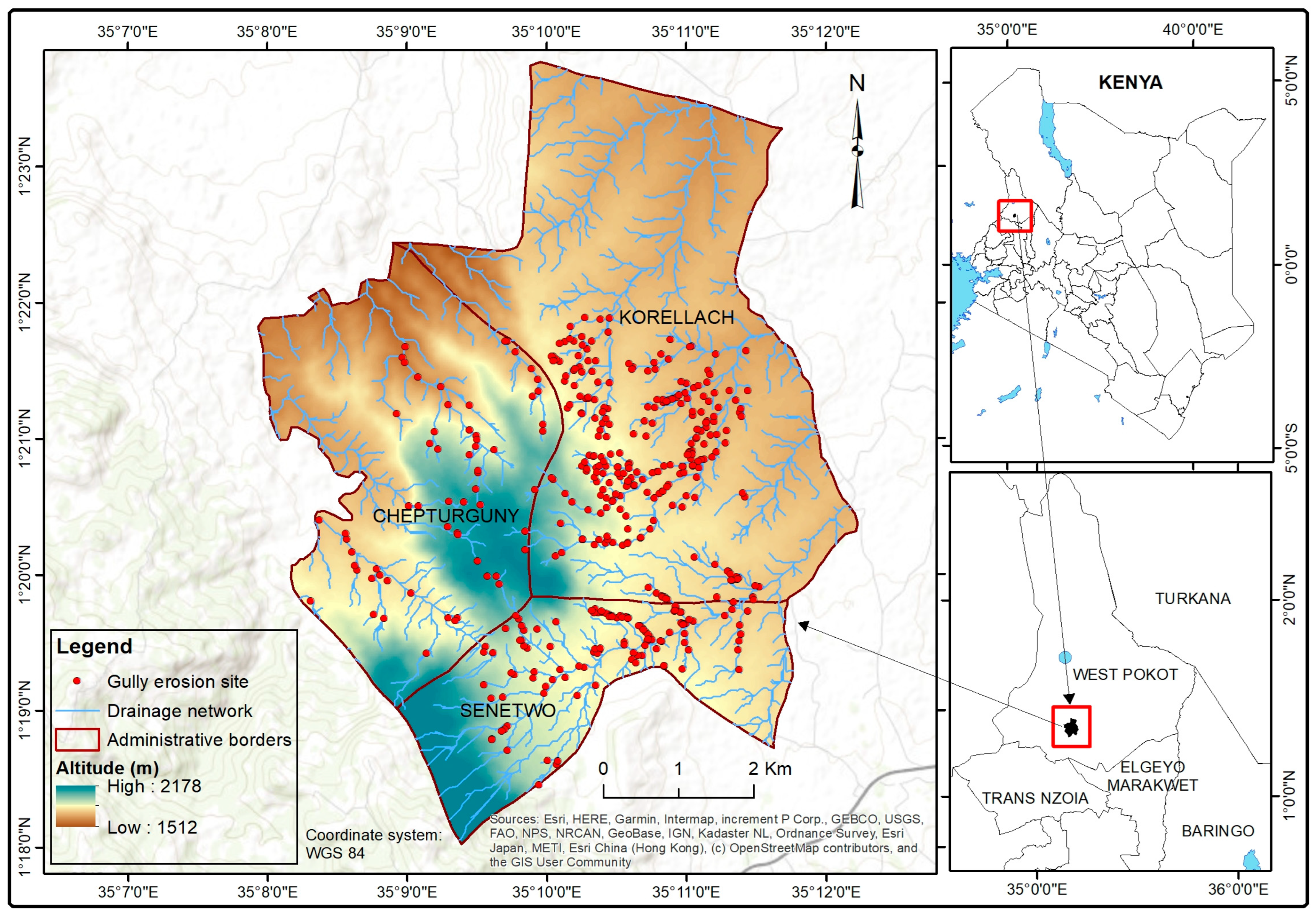
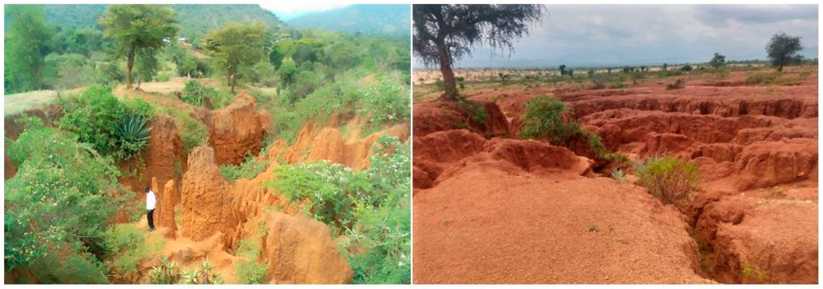
2.1. Description of the Study Area
2.2. Spatial Data Acquisition and Preparation
2.2.1. Gully Erosion Occurrence Data
2.2.2. Gully Erosion Conditioning Factors
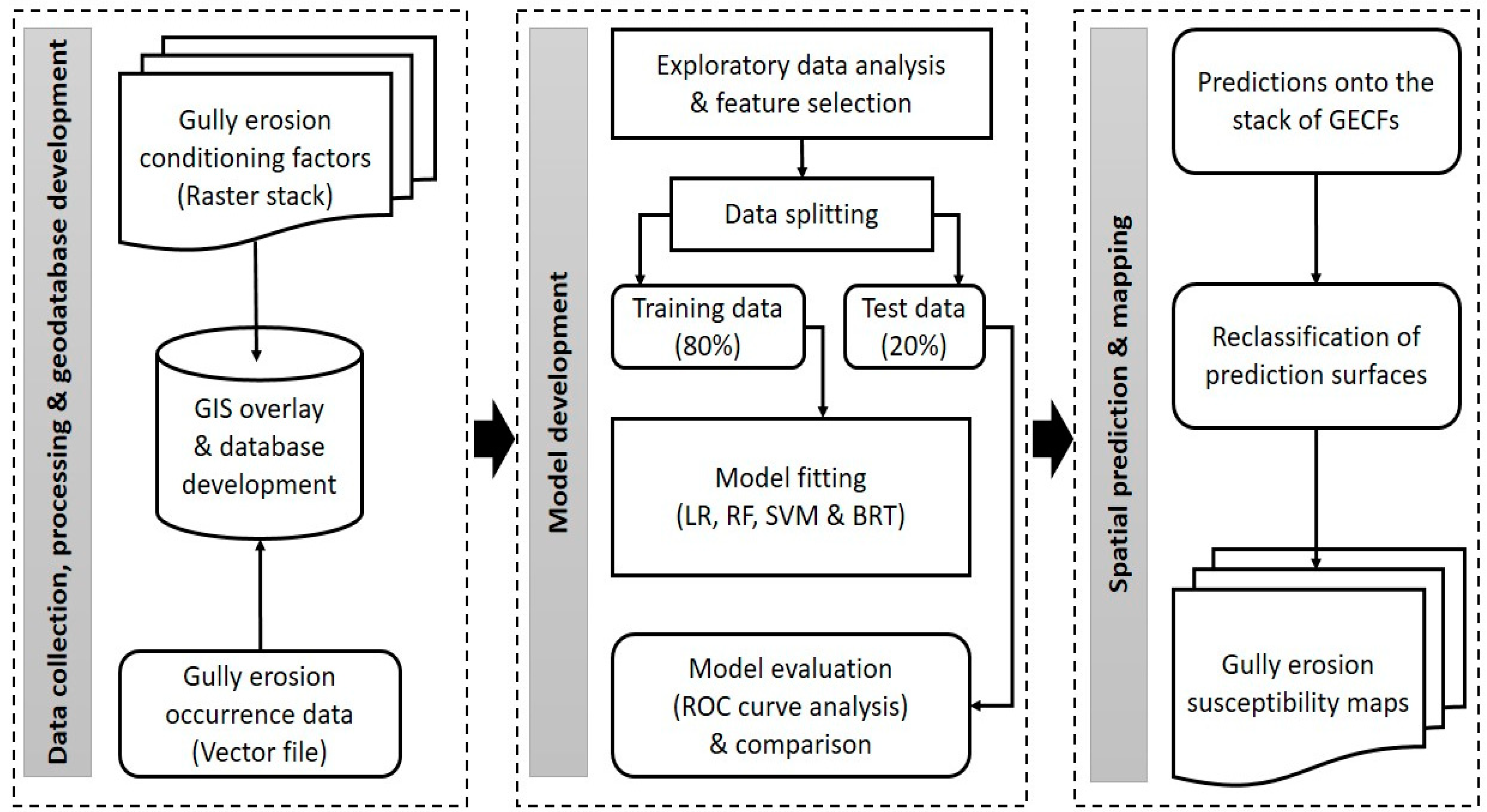
2.3. Spatial Modeling, Prediction and Mapping
2.3.1. Exploratory Data Analysis
2.3.2. Model Development
- Logistic regression
- Random forest
- Support vector machines
- Boosted regression trees
2.3.3. Model Evaluation and Comparison
2.3.4. Model Application
2.4. Software
3. Results
3.1. Exploratory Data Analysis
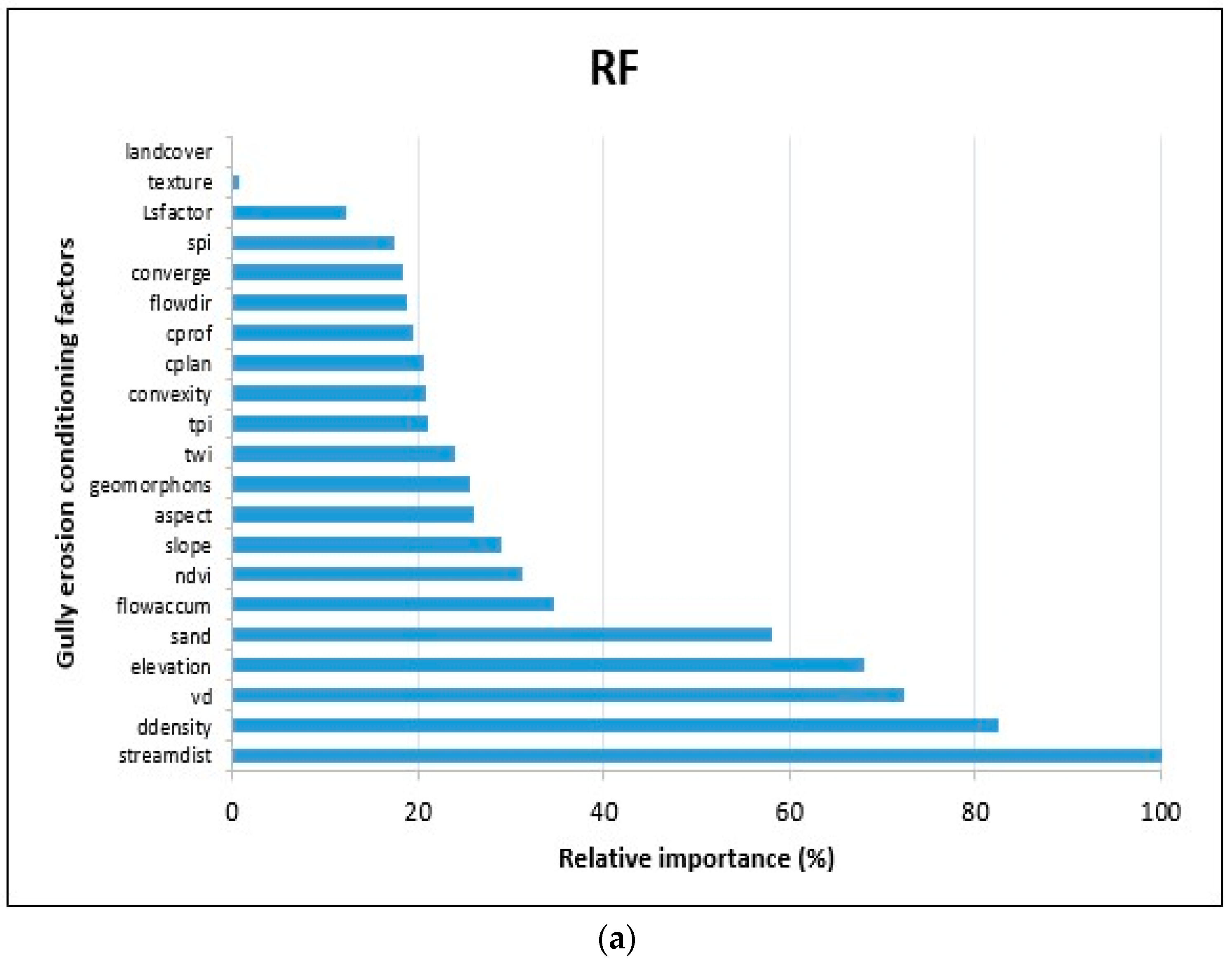
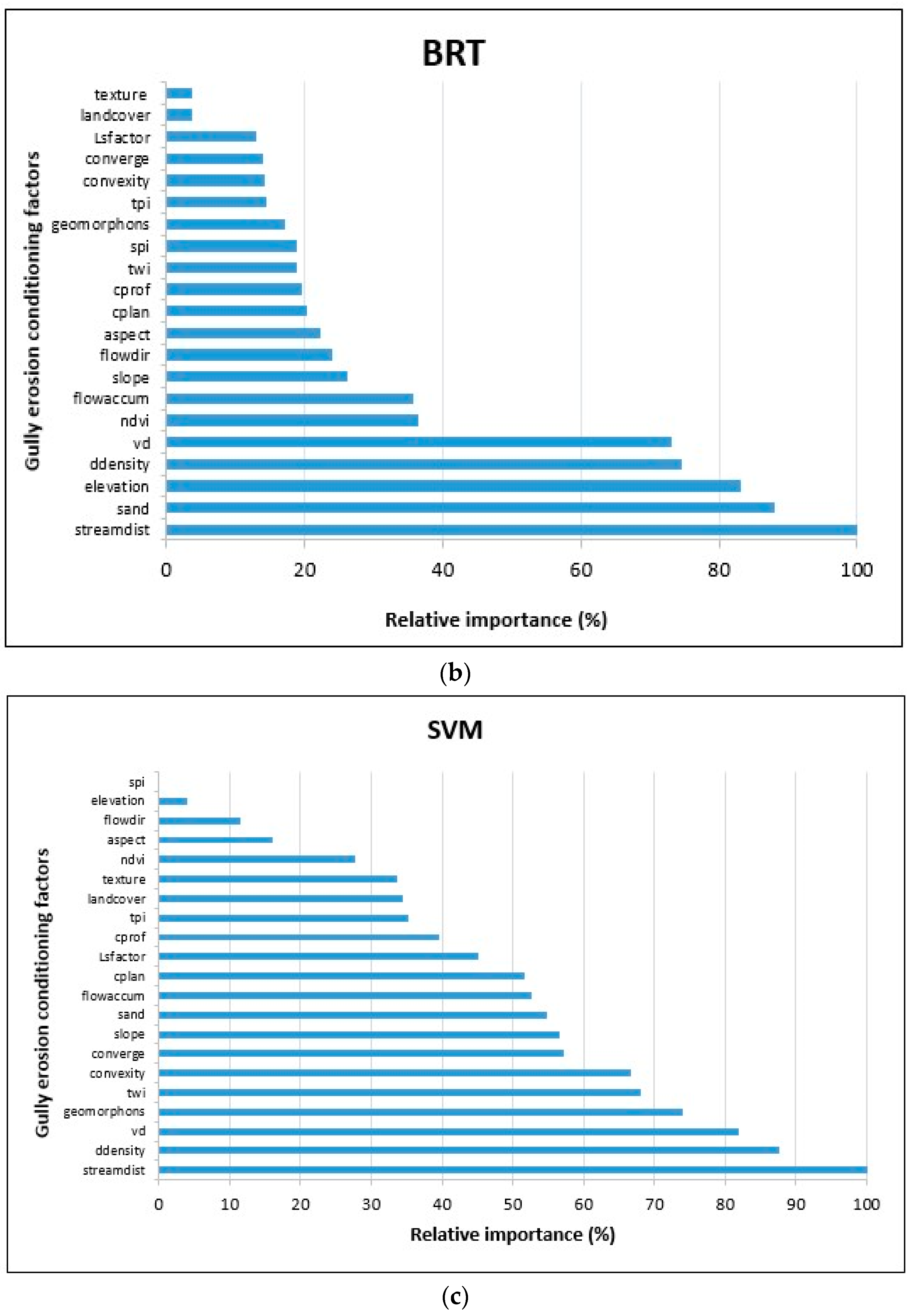
3.2. Models of Gully Erosion Susceptibility and Relative Importance of the Conditioning Factors
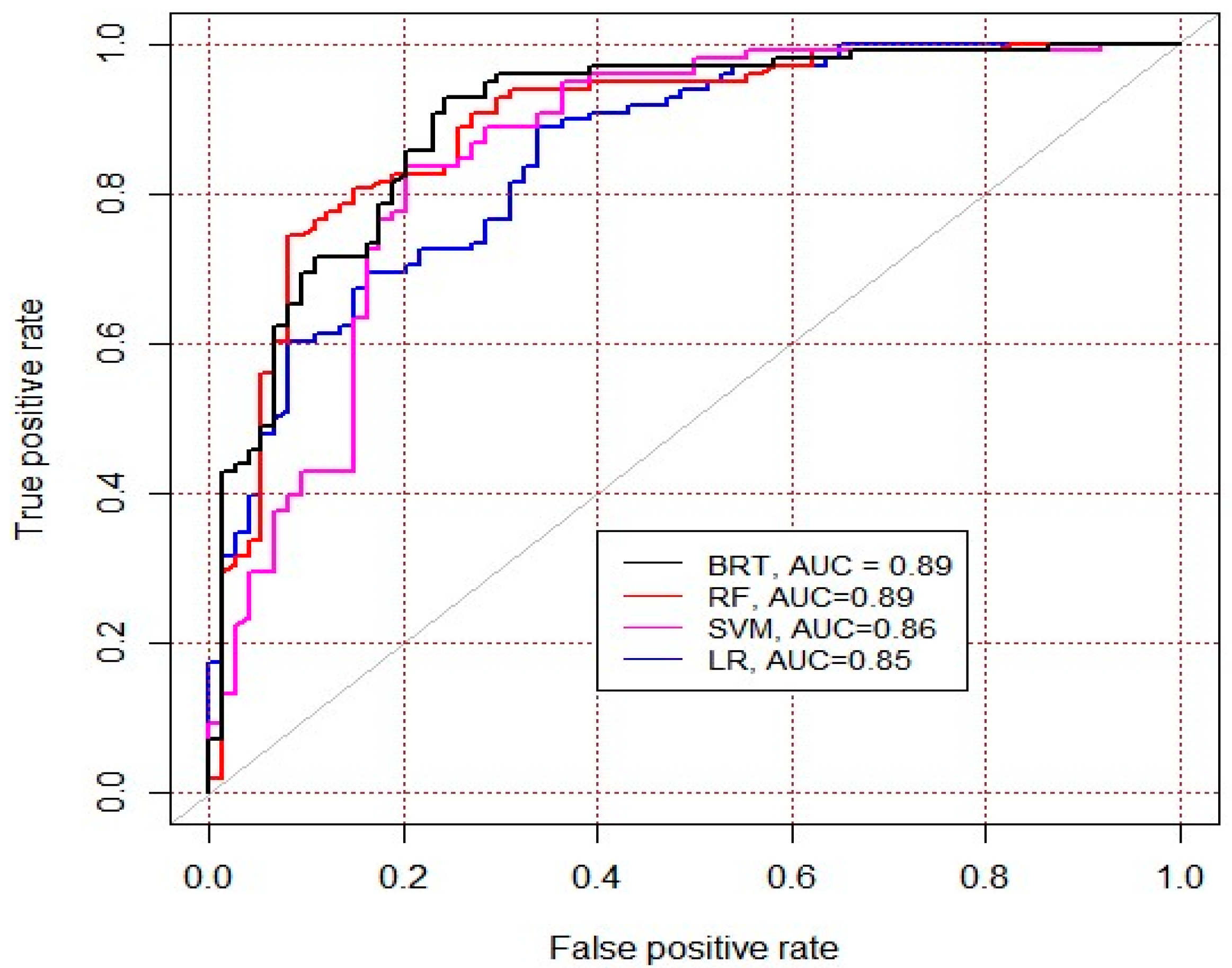
3.3. Model Evaluation and Comparison
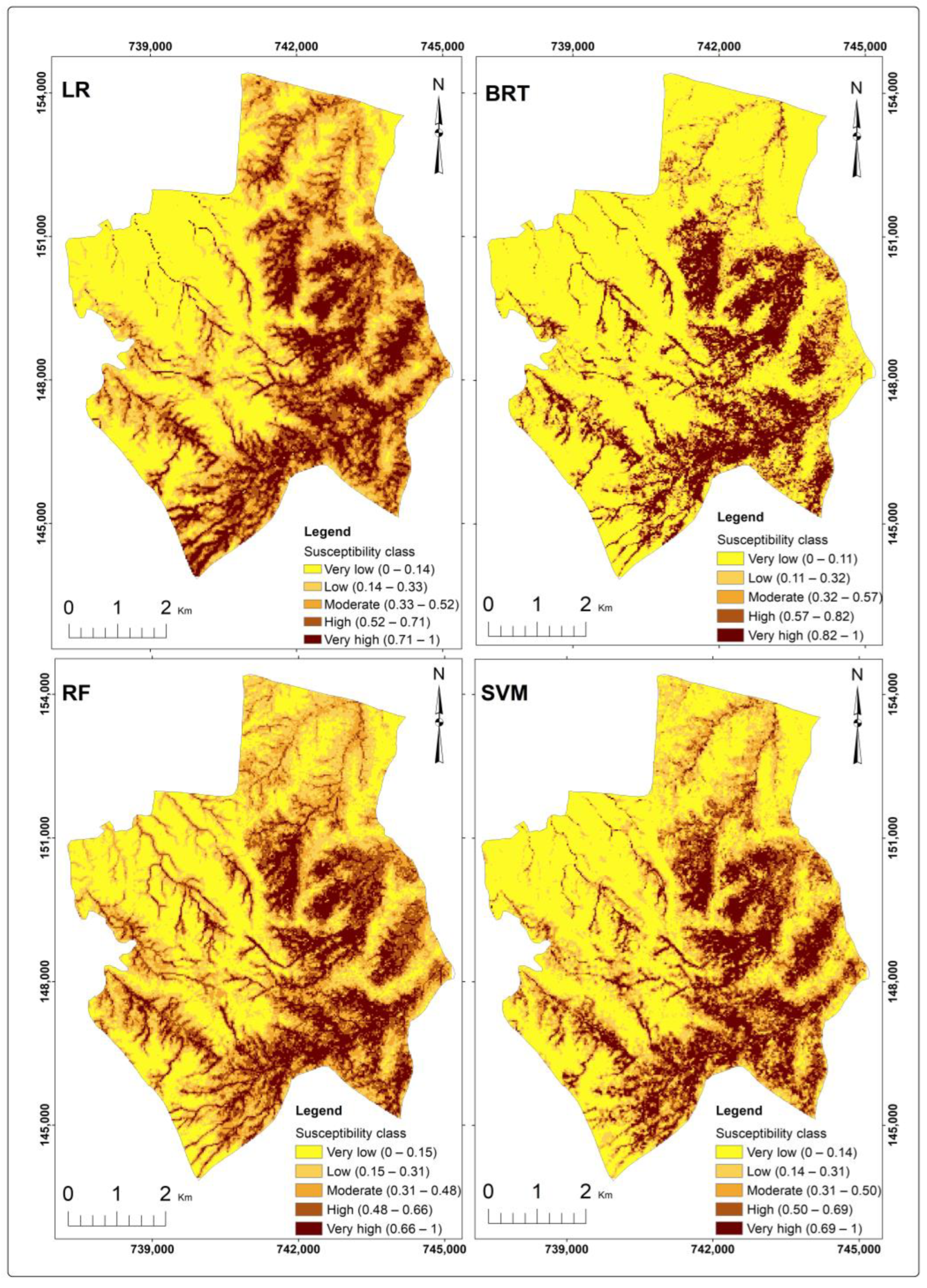
3.4. Spatial Patterns of Gully Erosion Susceptibility
4. Discussion
4.1. Relative Importance of the Gully Erosion Conditioning Factors
4.2. Model Evaluation and Comparison
5. Conclusions and Outlook
Author Contributions
Funding
Data Availability Statement
Acknowledgments
Conflicts of Interest
References
- Lorenz, K.; Lal, R.; Ehle, K. Soil organic carbon stock as an indicator for monitoring land and soil degradation in relation to United Nations’ Sustainable Development Goals. Land Degrad. Dev. 2019, 30, 824–838. [Google Scholar] [CrossRef]
- FAO and ITPS. Status of the World’s Soil Resources—Main Report; Food and Agriculture Organization of the United Nations and Intergovernmental Technical Panel on Soils: Rome, Italy, 2021; Available online: https://www.fao.org/documents/card/en/c/c6814873-efc3-41db-b7d3-2081a10ede50/ (accessed on 25 August 2021).
- UNCCD. The Global Land Outlook, 1st ed.; United Nations Conventions to Combat Desertification: Bonn, Germany, 2017; Available online: https://www.unccd.int/sites/default/files/documents/2017-09/GLO_Full_Report_low_res.pdf (accessed on 10 April 2023).
- Rahmati, O.; Tahmasebipour, N.; Haghizadeh, A.; Pourghasemi, H.R.; Feizizadeh, B. Evaluating the influence of geo-environmental factors on gully erosion in a semi-arid region of Iran: An integrated framework. Sci. Total Environ. 2017, 579, 913–927. [Google Scholar] [CrossRef]
- Arabameri, A.; Cerda, A.; Tiefenbacher, J.P. Spatial pattern analysis and prediction of gully erosion using novel hybrid model of entropy-weight of evidence. Water 2019, 11, 1129. [Google Scholar] [CrossRef] [Green Version]
- Conforti, M.; Aucelli, P.P.C.; Robustelli, G.; Scarciglia, F. Geomorphology and GIS analysis for mapping gully erosion susceptibility in the Turbolo stream catchment (Northern Calabria, Italy). Nat. Hazards 2011, 56, 881–898. [Google Scholar] [CrossRef]
- Conoscenti, C.; Agnesi, V.; Angileri, S.; Cappadonia, C.; Rotigliano, E.; Märker, M. A GIS-based approach for gully erosion susceptibility modelling: A test in Sicily, Italy. Env. Earth Sci. 2013, 70, 1179–1195. [Google Scholar] [CrossRef]
- Ireri, C.; Krhoda, G.O.; Mukhovi, M.S. Bivariate-based susceptibility mapping for gully erosion in Wanjoga River catchment Upper Tana Basin, Kenya. East Afr. J. Sci. Technol. Innov. 2021, 2, 1–15. [Google Scholar] [CrossRef]
- Busch, R.; Hardt, J.; Nir, N.; Schütt, B. Modeling gully erosion susceptibility to evaluate human impact on a local landscape system in Tigray, Ethiopia. Remote Sens. 2021, 13, 2009. [Google Scholar] [CrossRef]
- Roy, J.; Saha, S. Ensemble hybrid machine learning methods for gully erosion susceptibility mapping: K-fold cross validation approach. Artif. Intell. Geosci. 2022, 3, 28–45. [Google Scholar] [CrossRef]
- Zabihi, M.; Mirchooli, F.; Motevalli, A.; Khaledi, D.A.; Pourghasemi, H.R.; Zakeri, M.A.; Sadighi, F. Spatial modelling of gully erosion in Mazandaran Province, northern Iran. Catena 2018, 161, 1–13. [Google Scholar] [CrossRef]
- Vanmaercke, M.; Panagos, P.; Vanwalleghem, T.; Hayas, A.; Foerster, S.; Borrelli, P.; Rossi, M.; Torri, D.; Casali, J.; Borselli, L.; et al. Measuring, modelling and managing gully erosion at large scales: A state of the art. Earth-Sci. Rev. 2021, 218, 103637. [Google Scholar] [CrossRef]
- Dewitte, O.; Daoudi, M.; Bosco, C.; Eeckhaut, M.V.D. Predicting the susceptibility to gully initiation in data-poor regions. Geomorphology 2015, 228, 101–115. [Google Scholar] [CrossRef]
- Arabameri, A.; Rezaei, K.; Pourghasemi, H.R.; Lee, S.; Yamani, M. GIS-based gully erosion susceptibility mapping: A comparison among three data-driven models and AHP knowledge-based technique. Environ. Earth Sci. 2018, 77, 628. [Google Scholar] [CrossRef]
- Pal, S.C.; Arabameri, A.; Blaschke, T.; Chowdhuri, I.; Saha, A.; Chakrabortty, R.; Lee, S.; Band, S.S. Ensemble of machine-learning methods for predicting gully erosion susceptibility. Remote Sens. 2020, 12, 3675. [Google Scholar] [CrossRef]
- Yazie, T.; Mekonnen, M.; Derebe, A. Gully erosion and its impacts on soil loss and crop yield in three decades, northwest Ethiopia. Model. Earth Syst. Environ. 2021, 7, 2491–2500. [Google Scholar] [CrossRef]
- Igwe, O.; Ikechukwu, J.U.; Onwuka, S.; Ozioko, O. GIS-based gully erosion susceptibility modeling, adapting bivariate statistical method and AHP approach in Gombe town and environs Northeast Nigeria. Geoenviron. Disasters 2020, 7, 32. [Google Scholar] [CrossRef]
- Conoscenti, C.; Angileri, S.; Cappadonia, C.; Rotigliano, E.; Agnesi, V.; Märker, M. Gully erosion susceptibility assessment by means of GIS-based logistic regression: A case of Sicily (Italy). Geomorphology 2014, 204, 399–411. [Google Scholar] [CrossRef] [Green Version]
- Conoscenti, C.; Agnesi, V.; Cama, M.; Caraballo-Arias, N.A.; Rotigliano, E. Assessment of gully erosion susceptibility using multivariate adaptive regression splines and accounting for hydrological connectivity. Land Degrad. Dev. 2018, 29, 724–736. [Google Scholar] [CrossRef]
- Rahmati, O.; Haghizadeh, A.; Pourghasemi, H.R.; Noormohamadi, F. Gully erosion susceptibility mapping: The role of GIS-based bivariate statistical models and their comparison. Nat. Hazards 2016, 82, 1231–1258. [Google Scholar] [CrossRef]
- Javidan, N.; Kavian, A.; Pourghasemi, H.R.; Conoscenti, C.; Jafarian, Z. Gully erosion susceptibility mapping using multivariate adaptive regression splines-replications and sample size scenarios. Water 2019, 11, 2319. [Google Scholar] [CrossRef] [Green Version]
- Razavi-Termeh, S.V.; Sadeghi-Niaraki, A.; Choi, S. Gully erosion susceptibility mapping using artificial intelligence and statistical models. Geomat. Nat. Hazards Risk 2020, 11, 821–844. [Google Scholar] [CrossRef]
- Arabameri, A.; Pradhan, B.; Pourghasemi, H.R.; Rezaei, K.; Kerle, N. Spatial modelling of gully erosion using GIS and R programing: A comparison among three data mining algorithms. Appl. Sci. 2018, 8, 1369. [Google Scholar] [CrossRef] [Green Version]
- Avand, M.; Janizadeh, S.; Naghibi, S.A.; Pourghasemi, H.R.; Bozchaloei, S.K.; Blaschke, T. A comparative assessment of random forest and k-nearest neighbor classifiers for gully erosion susceptibility mapping. Water 2019, 11, 2076. [Google Scholar] [CrossRef] [Green Version]
- Tien Bui, D.; Shirzadi, A.; Shahabi, H.; Chapi, K.; Omidavr, E.; Thai Pham, B.; Asl, D.T.; Khaledian, H.; Pradhan, B.; Panahi, M.; et al. A novel ensemble artificial intelligence approach for gully erosion mapping in a semi-arid watershed (Iran). Sensors 2019, 19, 2444. [Google Scholar] [CrossRef] [Green Version]
- Band, S.S.; Janizadeh, S.; Pal, S.C.; Saha, A.; Chakrabortty, R.; Shokri, M.; Mosavi, A. Novel ensemble approach of Deep Learning Neural Network (DLNN) model and Particle Swarm Optimization (PSO) algorithm for prediction of gully erosion susceptibility. Sensors 2020, 20, 5609. [Google Scholar] [CrossRef] [PubMed]
- Ghorbanzadeh, O.; Shahabi, H.; Mirchooli, F.; Kamran, K.V.; Lim, S.; Aryal, J.; Jarihani, B.; Blaschke, T. Gully erosion susceptibility mapping (GESM) using machine learning methods optimized by the multi-collinearity analysis and K-fold cross-validation. Geomat. Nat. Hazards Risk 2020, 11, 1653–1678. [Google Scholar] [CrossRef]
- Lei, X.; Chen, W.; Avand, M.; Janizadeh, S.; Kariminejad, N.; Shahabi, H.; Costache, R.; Shahabi, H.; Shirzadi, A.; Mosavi, A. GIS-based machine learning algorithms for gully erosion susceptibility mapping in a semi-arid region of Iran. Remote Sens. 2020, 12, 2478. [Google Scholar] [CrossRef]
- Nhu, V.; Janizadeh, S.; Avand, M.; Chen, W.; Farzin, M.; Omidvar, E.; Shirzadi, A.; Shahabi, H.; Clague, J.J.; Jaafari, A.; et al. GIS-Based Gully erosion susceptibility mapping: A comparison of computational ensemble data mining models. Appl. Sci. 2020, 10, 2039. [Google Scholar] [CrossRef] [Green Version]
- Pourghasemi, H.R.; Yousefi, S.; Kornejady, A.; Cerdà, A. Performance assessment of individual and ensemble data-mining techniques for gully erosion modeling. Sci. Total Environ. 2017, 609, 764–775. [Google Scholar] [CrossRef] [Green Version]
- Pourghasemi, H.R.; Sadhasivam, N.; Kariminejad, N.; Collins, A.L. Gully erosion spatial modelling: Role of machine learning algorithms in selection of the best controlling factors and modelling process. Geosci. Front. 2020, 11, 2207–2219. [Google Scholar] [CrossRef]
- Ahmadpour, H.; Bazrafshan, O.; Rafiei-Sardooi, E.; Zamani, H.; Panagopoulos, T. Gully erosion susceptibility assessment in the Kondoran watershed using machine learning algorithms and the Boruta feature selection. Sustainability 2021, 13, 10110. [Google Scholar] [CrossRef]
- Arabameri, A.; Pal, S.C.; Costache, R.; Saha, A.; Rezaie, F.; Danesh, A.S.; Pradhan, B.; Lee, S.; Hoang, N. Prediction of gully erosion susceptibility mapping using novel ensemble machine learning algorithms. Geomat. Nat. Hazards Risk 2021, 12, 469–498. [Google Scholar] [CrossRef]
- Saha, S.; Sarkar, R.; Thapa, G.; Roy, J. Modeling gully erosion susceptibility in Phuentsholing, Bhutan using deep learning and basic machine learning algorithms. Environ. Earth Sci. 2021, 80, 295. [Google Scholar] [CrossRef]
- Yang, A.; Wang, C.; Pang, G.; Long, Y.; Wang, L.; Cruse, R.M.; Yang, Q. Gully erosion susceptibility mapping in highly complex terrain using machine learning models. ISPRS Int. J. Geo-Inf. 2021, 10, 680. [Google Scholar] [CrossRef]
- Jaafari, A.; Janizadeh, S.; Abdo, H.G.; Mafi-Gholami, D.; Adeli, B. Understanding land degradation induced by gully erosion from the perspective of different geoenvironmental factors. J. Environ. Manag. 2022, 315, 115181. [Google Scholar] [CrossRef] [PubMed]
- Vanmaercke, M.; Chen, Y.; Haregeweyn, N.; De Geeter, S.; Campforts, B.; Heyndrickx, W.; Tsunekawa, A.; Poesen, J. Predicting gully densities at sub-continental scales: A case study for the Horn of Africa. Earth Surf. Process. Landf. 2020, 45, 3763–3779. [Google Scholar] [CrossRef]
- County Government of West Pokot. County Integrated Development Plan (2018–2022). 256p. Available online: https://www.devolution.go.ke/wp-content/uploads/2020/02/Westpokot-CIDP-2018-2022.pdf (accessed on 25 August 2021).
- Reith, J.; Ghazaryan, G.; Muthoni, F.; Dubovyk, O. Assessment of land degradation in semiarid Tanzania—Using multiscale remote sensing datasets to support sustainable development goal 15.3. Remote Sens. 2021, 13, 1754. [Google Scholar] [CrossRef]
- Wairore, J.N.; Mureithi, S.M.; Wasonga, O.V.; Nyberg, G. Characterization of enclosure management regimes and factors influencing their choice among agro-pastoralists in north-western Kenya. Pastor. Res. Policy Pract. 2015, 5, 14. [Google Scholar] [CrossRef] [Green Version]
- Wairore, J.N.; Mureithi, S.M.; Wasonga, O.V.; Nyberg, G. Benefits derived from rehabilitating a degraded semi-arid rangeland in private enclosures in West Pokot County, Kenya. Land Degrad. Dev. 2015, 27, 532–541. [Google Scholar] [CrossRef]
- Touber, L. Landforms and Soils of West Pokot District, Kenya: A Site Evaluation for Range-Land Use. Wageningen (The Netherlands), The Winand Staring Centre for Integrated Land, Soil and Water Research. Report No. 50. Available online: https://esdac.jrc.ec.europa.eu/content/landforms-and-soils-west-pokot-district-site-evaluation-rangeland-use-report-no-p50 (accessed on 25 August 2021).
- Arukulem, Y.E.; Makindi, S.M.; Obwoyere, G.O. Climate variability and the associated impacts on smallholder agriculture in Senetwo location, Kenya. Int. J. Sci. Res. 2015, 4, 845–850. [Google Scholar]
- Wilson, J.P.; Gallant, J.C. Terrain Analysis: Principles and Applications; John Wiley & Sons, Inc.: Hoboken, NJ, USA, 2000. [Google Scholar]
- Campbell, J.B. Introduction to Remote Sensing, 3rd ed.; Taylor & Francis: London, UK, 2002. [Google Scholar]
- Lillesand, T.M.; Kiefer, R.W.; Chipman, J.W. Remote Sensing and Image Interpretation, 6th ed.; John Wiley & Sons, Inc.: Hoboken, NJ, USA, 2008. [Google Scholar]
- Menard, S. Applied Logistic Regression Analysis, Quantitative Applications in the Social Sciences; No. 106; Sage: London, UK, 2002. [Google Scholar]
- Montgomery, D.C.; Peck, E.A.; Vining, G.G. Introduction to Linear Regression Analysis; Wiley: Hoboken, NJ, USA, 2006. [Google Scholar]
- Agresti, A. An Introduction to Categorical Data Analysis; Wiley: Hoboken, NJ, USA, 2007. [Google Scholar]
- Cutler, A.; Cutler, D.R.; Stevens, J.R. Random Forests. In Ensemble Machine Learning: Methods and Applications; Zhang, C., Ma, Y., Eds.; Springer: New York, NY, USA, 2012; pp. 157–175. [Google Scholar]
- Taalab, K.; Cheng, T.; Zhang, Y. Mapping landslide susceptibility and types using random forest. Big Earth Data 2018, 2, 159–178. [Google Scholar] [CrossRef]
- Arabameri, A.; Nalivan, O.A.; Saha, S.; Roy, J.; Pradhan, B.; Tiefenbacher, J.P.; Ngo, P.T.T. Novel ensemble approaches of machine learning techniques in modeling the gully erosion susceptibility. Remote Sens. 2020, 12, 1890. [Google Scholar] [CrossRef]
- Hong, H.; Pradhan, B.; Jebur, M.N.; Tien Bui, D.; Xu, C.; Akgun, A. Spatial prediction of landslide hazard at the Luxi area (China) using support vector machines. Environ. Earth Sci. 2016, 75, 40. [Google Scholar] [CrossRef]
- Tien Bui, D.; Pradhan, B.; Lofman, O.; Revhaug, I. Landslide susceptibility assessment in Vietnam using support vector machine, decision tree and Naïve Bayes models. Math. Prob. Eng. 2012, 974638. [Google Scholar] [CrossRef] [Green Version]
- Pradhan, B. A comparative study on the predictive ability of the decision tree, support vector machine and neuro-fuzzy models in landslide susceptibility mapping using GIS. Comput. Geosci. 2013, 51, 350–365. [Google Scholar] [CrossRef]
- Kavzoglu, T.; Colkesen, I. A kernel function analysis for support vector machines for land cover classification. Int. J. Appl. Earth Observ. Geoinfomat. 2009, 11, 352–359. [Google Scholar] [CrossRef]
- Elith, J.; Leathwick, J.R.; Hastie, T.A. Working guide to boosted regression trees. J. Anim. Ecol. 2008, 77, 802–813. [Google Scholar] [CrossRef]
- Ließ, M.; Schmidt, J.; Glaser, B. Improving the spatial prediction of soil organic carbon stocks in a complex tropical mountain landscape by methodological specifications in machine learning approaches. PLoS ONE 2016, 11, e0153673. [Google Scholar] [CrossRef] [PubMed] [Green Version]
- Yang, R.; Zhang, G.; Liu, F.; Lu, Y.; Yang, F.; Yang, F.; Yang, M.; Zhao, Y.; Li, D. Comparison of boosted regression tree and random forest models for mapping topsoil organic carbon concentration in an alpine ecosystem. Ecol. Indic. 2016, 60, 870–878. [Google Scholar] [CrossRef]
- Pontius, R.G.; Schneider, L.C. Land cover change model validation by an ROC method for the Ipswich watershed, Massachusetts, USA. Agric. Ecosyst. Environ. 2001, 85, 239–248. [Google Scholar] [CrossRef]
- Fawcett, T. An introduction to ROC analysis. Pattern Recognit. Lett. 2006, 27, 861–874. [Google Scholar] [CrossRef]
- Metz, C.E. Basic principles of ROC analysis. Seminars in Nuclear Science III 1978, 8, 283–298. [Google Scholar] [CrossRef] [PubMed]
- Hosmer, D.W.; Lemeshow, S. Applied Logistic Regression; Wiley Series in Probability and Statistics; Wiley: Hoboken, NJ, USA, 2000. [Google Scholar] [CrossRef]
- R Development Core Team. R: A Language and Environment for Statistical Computing; R Foundation for Statistical Computing: Vienna, Austria, 2020. [Google Scholar]
- Chuma, G.B.; Mugumaarhahama, Y.; Mond, J.M.; Bagula, E.M.; Ndeko, A.B.; Lucungu, P.B.; Karume, K.; Mushagalusa, G.N.; Schmitz, S. Gully erosion susceptibility mapping using four machine learning methods in Luzinzi watershed, eastern Democratic Republic of Congo. Phys. Chem. Earth 2023, 129, 103295. [Google Scholar] [CrossRef]
- Arabameri, A.; Chen, W.; Loche, M.; Zhao, X.; Li, Y.; Lombardo, L.; Cerda, A.; Pradhan, B.; Tien Bui, D. Comparison of machine learning models for gully erosion susceptibility mapping. Geosci. Front. 2020, 11, 1609–1620. [Google Scholar] [CrossRef]
- Arabameri, A.; Blaschke, T.; Pradhan, B.; Pourghasemi, H.R.; Tiefenbacher, J.P.; Tien Bui, D. Evaluation of recent advanced soft computing techniques for gully erosion susceptibility mapping: A comparative study. Sensors 2020, 20, 335. [Google Scholar] [CrossRef] [Green Version]
- Amare, S.; Langendoen, E.; Keesstra, S.; van der Ploeg, M.; Gelagay, H.; Lemma, H.; van der Zee, S.E.A.T.M. Susceptibility to gully erosion: Applying random forest (RF) and frequency ratio (FR) approaches to a small catchment in Ethiopia. Water 2021, 13, 216. [Google Scholar] [CrossRef]
- Bouramtane, T.; Hilal, H.; Rezende-Filho, A.T.; Bouramtane, K.; Barbiero, L.; Abraham, S.; Valles, V.; Kacimi, I.; Sanhaji, H.; Torres-Rondon, L.; et al. Mapping gully erosion variability and susceptibility using remote sensing, multivariate statistical analysis, and machine learning in South Mato Grosso, Brazil. Geosciences 2022, 12, 235. [Google Scholar] [CrossRef]
- Garosi, Y.; Sheklabadi, M.; Conoscenti, C.; Pourghasemi, H.R.; van Oostef, K. Assessing the performance of GIS-based machine learning models with different accuracy measures for determining susceptibility to gully erosion. Sci. Total Environ. 2019, 664, 1117–1132. [Google Scholar] [CrossRef] [PubMed]
- Gayen, A.; Pourghasemi, H.R.; Saha, S.; Keesstra, S.; Bai, S. Gully erosion susceptibility assessment and management of hazard-prone areas in India using different machine learning algorithms. Sci. Total Environ. 2019, 668, 124–138. [Google Scholar] [CrossRef]
- Hembram, T.K.; Saha, S.; Pradhan, B.; Maulud, K.N.A.; Alamri, A.M. Robustness analysis of machine learning classifiers in predicting spatial gully erosion susceptibility with altered training samples. Geomat. Nat. Hazards Risk 2021, 12, 794–828. [Google Scholar] [CrossRef]
- Amiri, M.; Pourghasemi, H.R.; Ghanbarian, G.A.; Afzali, S.F. Assessment of the importance of gully erosion effective factors using Boruta algorithm and its spatial modeling and mapping using three machine learning algorithms. Geoderma 2019, 340, 55–69. [Google Scholar] [CrossRef]
- Rahmati, O.; Tahmasebipour, N.; Hamid, A.H.; Pourghasemi, H.R.; Feizizadeh, B. Evaluation of different machine learning models for predicting and mapping the susceptibility of gully erosion. Geomorphology 2017, 298, 118–137. [Google Scholar] [CrossRef]
- Wang, F.; Sahana, M.; Pahlevanzadeh, B.; Pal, S.C.; Shit, P.K.; Piran, M.J.; Janizadeh, S.; Band, S.S.; Mosavi, A. Applying different resampling strategies in machine learning models to predict head-cut gully erosion susceptibility: Predict head-cut gully erosion susceptibility. Alex. Eng. J. 2021, 60, 5813–5829. [Google Scholar] [CrossRef]
- Youssef, A.M.; Pourghasemi, H.R. Landslide susceptibility mapping using machine learning algorithms and comparison of their performance at Abha Basin, Asir Region, Saudi Arabia. Geosci. Front. 2021, 12, 639–655. [Google Scholar] [CrossRef]
- Saha, S.; Roy, J.; Arabameri, A.; Blaschke, T.; Tien Bui, D. Machine learning-based gully erosion susceptibility mapping: A case studyof eastern india. Sensors 2020, 20, 1313. [Google Scholar] [CrossRef] [PubMed] [Green Version]


| Factor | Scale | Proxy for/Effects | Source |
|---|---|---|---|
| Elevation (DEM) | 30 m | Micro-climate, vegetation, drainage network | https://earthexplorer.usgs.gov (Accessed on 1 August 2021) |
| Rainfall (1970–2000) | 1 km | Soil moisture, volume of surface runoff, sediment transport capacity, slope stability | https://worldclim.org (Accessed on 1 August 2021) |
| Slope angle (gradient) | 30 m | Overland and subsurface flows, erosive energy of overland flow, flow velocity, drainage density, sediment transport capacity, infiltration rate | DEM |
| Slope length-steepness (LS) factor | |||
| Flow accumulation | 30 m | Soil moisture (saturation), surface runoff | DEM |
| Topographic wetness index | |||
| Slope aspect | 30 m | Evapotranspiration, soil moisture, vegetation structure, weathering rate, micro-climate | DEM |
| Plan curvature | 30 m | Concentration of overland flow, flow velocity (rate) | DEM |
| Profile curvature | |||
| Convexity | |||
| Convergence index | |||
| Terrain ruggedness index | |||
| Topographic position index | |||
| Geomorphons | |||
| Landform | |||
| Texture | |||
| Valley depth | |||
| Stream power index | 30 m | Stream incision, slope erosion | DEM |
| Land use/cover | 30 m | Slope stability, evapotranspiration, infiltration, overland flow, surface runoff generation, sediment dynamics | Landsat 8 OLI imagery https://earthexplorer.usgs.gov (Accessed on 1 August 2021) |
| NDVI | |||
| Drainage density | 30 m | Flow magnitude, sediment transport capacity, infiltration, surface runoff | DEM |
| Distance to stream | |||
| Clay content | 0–20 cm depth | Infiltration rate, surface runoff, erosion resistance, subsurface flow and piping | https://isda-africa.com/isdasoil (Accessed on 1 August 2021) |
| Sand content |
| Predicted | |||
|---|---|---|---|
| Observed | Presence (1) | Absence (0) | |
| Presence (1) | TP (1|1) | FN (1|0) | |
| Absence (0) | FP (0|1) | TN (0|0) | |
| Factor | VIF | Factor | VIF | Factor | VIF |
|---|---|---|---|---|---|
| Aspect | 1.28 | LS Factor | 5.51 | Flow direction | 1.18 |
| Convergence index | 2.49 | NDVI | 2.86 | Flow accumulation | 1.23 |
| Convexity | 1.46 | Sand content | 3.49 | Geomorphons | 2.41 |
| Plan curvature | 3.57 | Slope gradient | 2.25 | Land cover | 2.25 |
| Profile curvature | 1.85 | Stream power index | 1.62 | Topographic position index | 1.97 |
| Drainage density | 1.54 | Distance to stream | 1.61 | Topographic wetness index | 1.75 |
| Elevation | 3.07 | Texture (SAGA) | 1.25 | Valley depth | 2.58 |
| Parameter | Estimate | Std. Error | Odds Ratio | p Value |
|---|---|---|---|---|
| (Intercept) | −36.1502 | 5.0454 | 0.0000 | 0.0000 |
| Plan curvature | −148.9885 | 42.8495 | 0.0000 | 0.0005 |
| Drainage density | 0.1991 | 0.0554 | 1.2203 | 0.0003 |
| Sand content | 0.1879 | 0.0276 | 1.2067 | 0.0000 |
| Elevation | 0.0137 | 0.0022 | 1.0138 | 0.0000 |
| Valley depth | 0.0165 | 0.0036 | 1.0167 | 0.0000 |
| Distance to stream | −0.0095 | 0.0029 | 0.9906 | 0.0009 |
| Slope gradient | −2.9885 | 1.3371 | 0.0504 | 0.0254 |
| Stream power index | 0.0001 | 0.0000 | 1.0001 | 0.0227 |
| Pr > LRo | 0.0000 | |||
| Pr > HL | 0.7072 |
| Model | Predicted | |||
|---|---|---|---|---|
| Observed | Presence | Absence | % Correct | |
| LR | Presence | 80 | 18 | 81.6 a |
| Absence | 25 | 49 | 66.2 b | |
| Overall accuracy (%) | 79.6 | |||
| SVM | Presence | 79 | 19 | 80.6 a |
| Absence | 16 | 58 | 78.4 b | |
| Overall accuracy (%) | 79.1 | |||
| BRT | Presence | 77 | 21 | 78.6 a |
| Absence | 14 | 60 | 81.1 b | |
| Overall accuracy (%) | 79.7 | |||
| RF | Presence | 80 | 18 | 81.6 a |
| Absence | 16 | 58 | 78.4 b | |
| Overall accuracy (%) | 80.2 | |||
| Class | LR | BRT | RF | SVM | ||||
|---|---|---|---|---|---|---|---|---|
| Area (km2) | % | Area (km2) | % | Area (km2) | % | Area (km2) | % | |
| Very low | 14.81 | 30.41 | 27.06 | 55.56 | 13.12 | 26.95 | 18.07 | 37.10 |
| Low | 9.66 | 19.84 | 5.80 | 11.91 | 11.56 | 23.73 | 9.59 | 19.69 |
| Moderate | 8.90 | 18.28 | 4.18 | 8.59 | 9.77 | 20.06 | 7.46 | 15.32 |
| High | 8.79 | 18.04 | 4.15 | 8.51 | 8.59 | 17.63 | 7.12 | 14.61 |
| Very high | 6.54 | 13.43 | 7.52 | 15.43 | 5.66 | 11.63 | 6.47 | 13.28 |
| Total | 48.71 | 100.00 | 48.71 | 100.00 | 48.71 | 100.00 | 48.71 | 100.00 |
Disclaimer/Publisher’s Note: The statements, opinions and data contained in all publications are solely those of the individual author(s) and contributor(s) and not of MDPI and/or the editor(s). MDPI and/or the editor(s) disclaim responsibility for any injury to people or property resulting from any ideas, methods, instructions or products referred to in the content. |
© 2023 by the authors. Licensee MDPI, Basel, Switzerland. This article is an open access article distributed under the terms and conditions of the Creative Commons Attribution (CC BY) license (https://creativecommons.org/licenses/by/4.0/).
Share and Cite
Were, K.; Kebeney, S.; Churu, H.; Mutio, J.M.; Njoroge, R.; Mugaa, D.; Alkamoi, B.; Ng’etich, W.; Singh, B.R. Spatial Prediction and Mapping of Gully Erosion Susceptibility Using Machine Learning Techniques in a Degraded Semi-Arid Region of Kenya. Land 2023, 12, 890. https://doi.org/10.3390/land12040890
Were K, Kebeney S, Churu H, Mutio JM, Njoroge R, Mugaa D, Alkamoi B, Ng’etich W, Singh BR. Spatial Prediction and Mapping of Gully Erosion Susceptibility Using Machine Learning Techniques in a Degraded Semi-Arid Region of Kenya. Land. 2023; 12(4):890. https://doi.org/10.3390/land12040890
Chicago/Turabian StyleWere, Kennedy, Syphyline Kebeney, Harrison Churu, James Mumo Mutio, Ruth Njoroge, Denis Mugaa, Boniface Alkamoi, Wilson Ng’etich, and Bal Ram Singh. 2023. "Spatial Prediction and Mapping of Gully Erosion Susceptibility Using Machine Learning Techniques in a Degraded Semi-Arid Region of Kenya" Land 12, no. 4: 890. https://doi.org/10.3390/land12040890