
Risk Assessment of Earthquake–Landslide Hazard Chain Based on CF-SVM and Newmark Model—Using Changbai Mountain as an Example

 , ,
, ,
Abstract
:1. Introduction
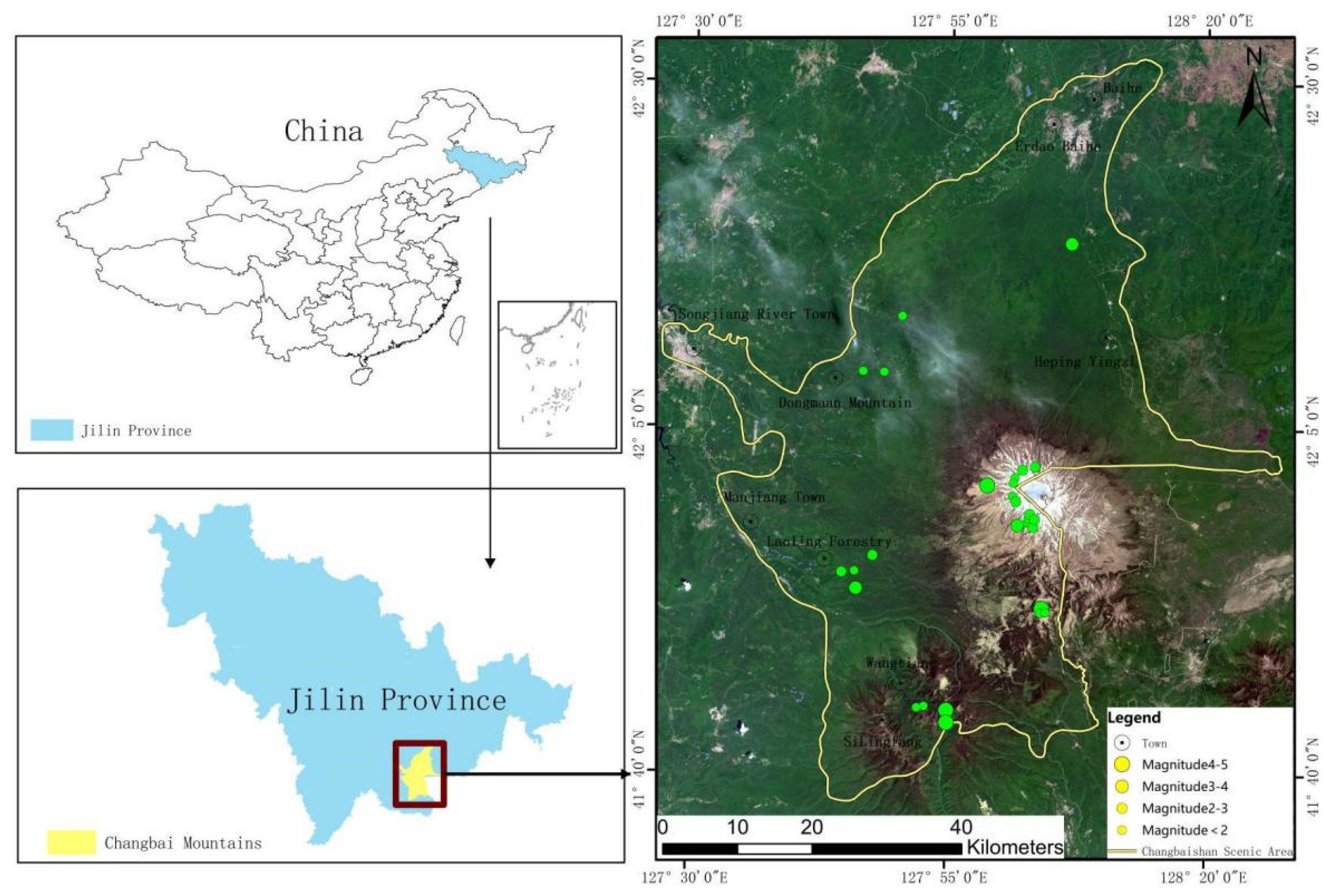
2. Study Area
3. Data and Methods
3.1. Certainty Factor
3.2. Support Vector Machine (SVM)
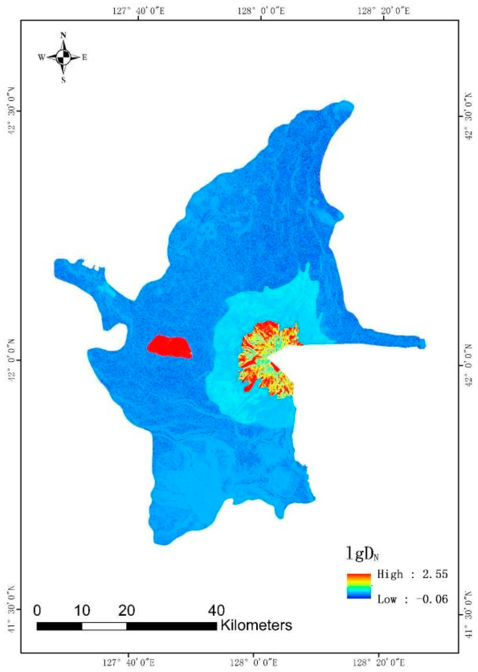
3.3. Newmark Model
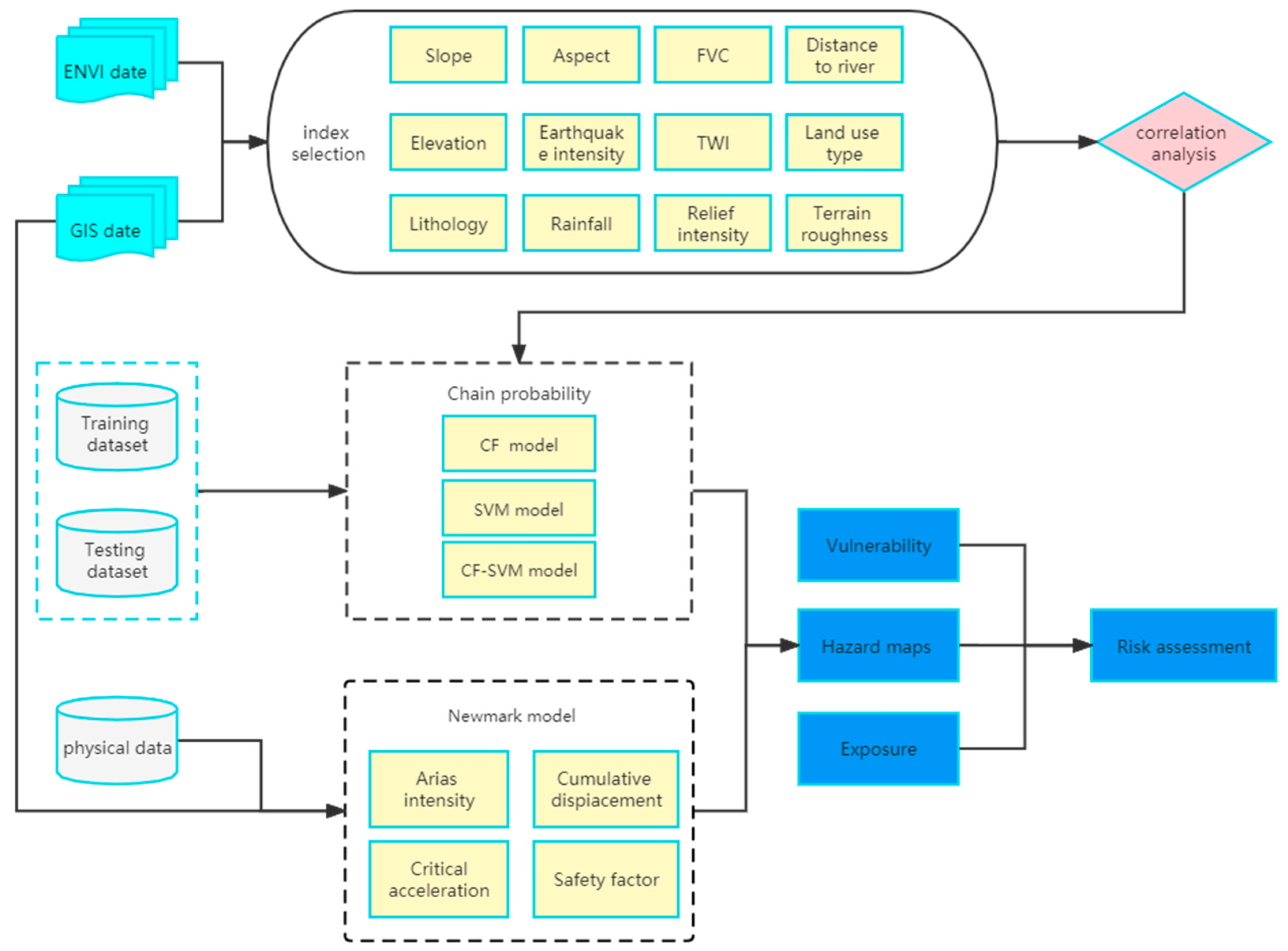
3.4. Risk Assessment Model of Earthquake-Induced Landslide Disaster Chain
4. Geological Hazard Susceptibility Assessment Results
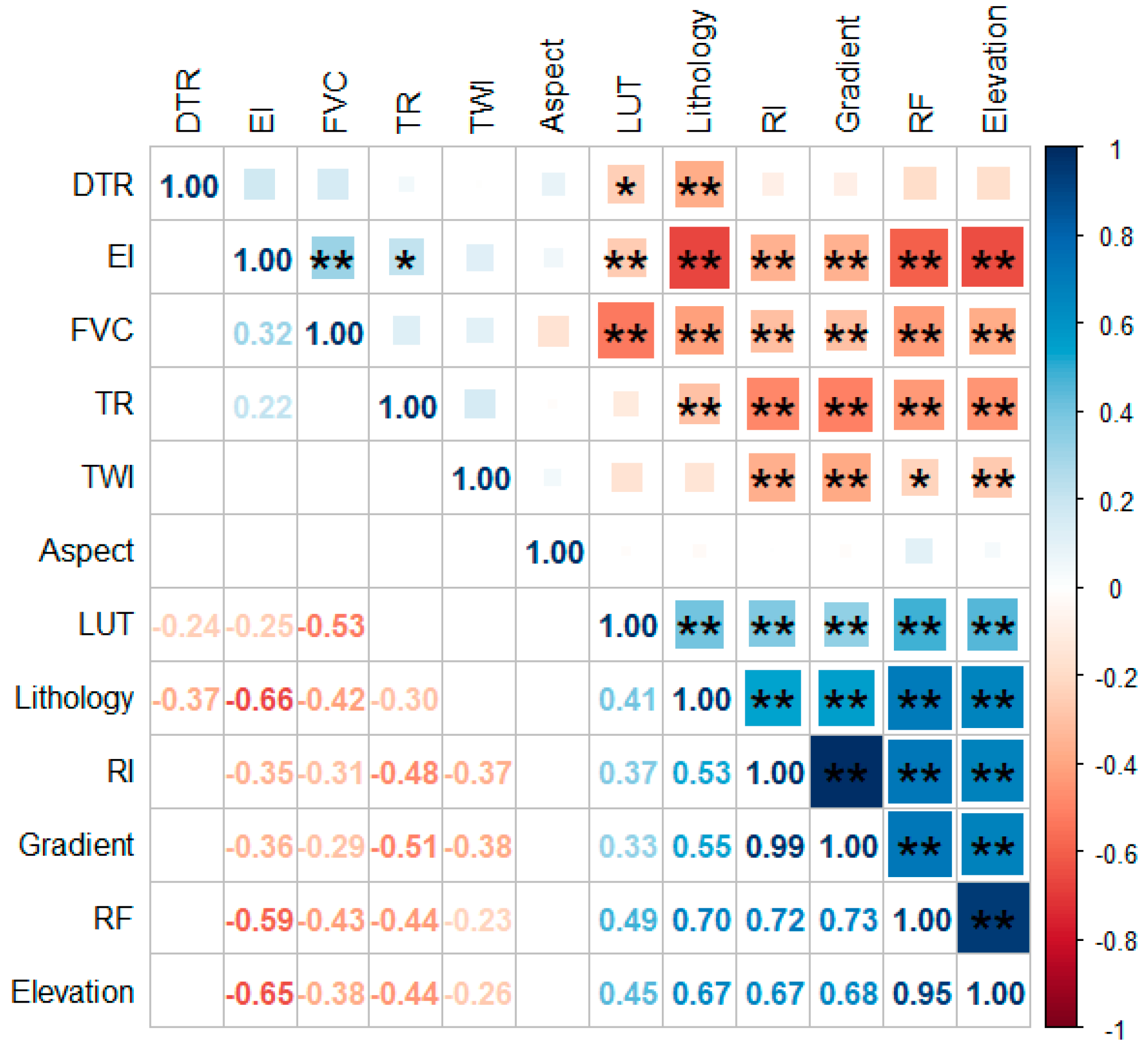
4.1. Correlation Analysis of Evaluation Factors
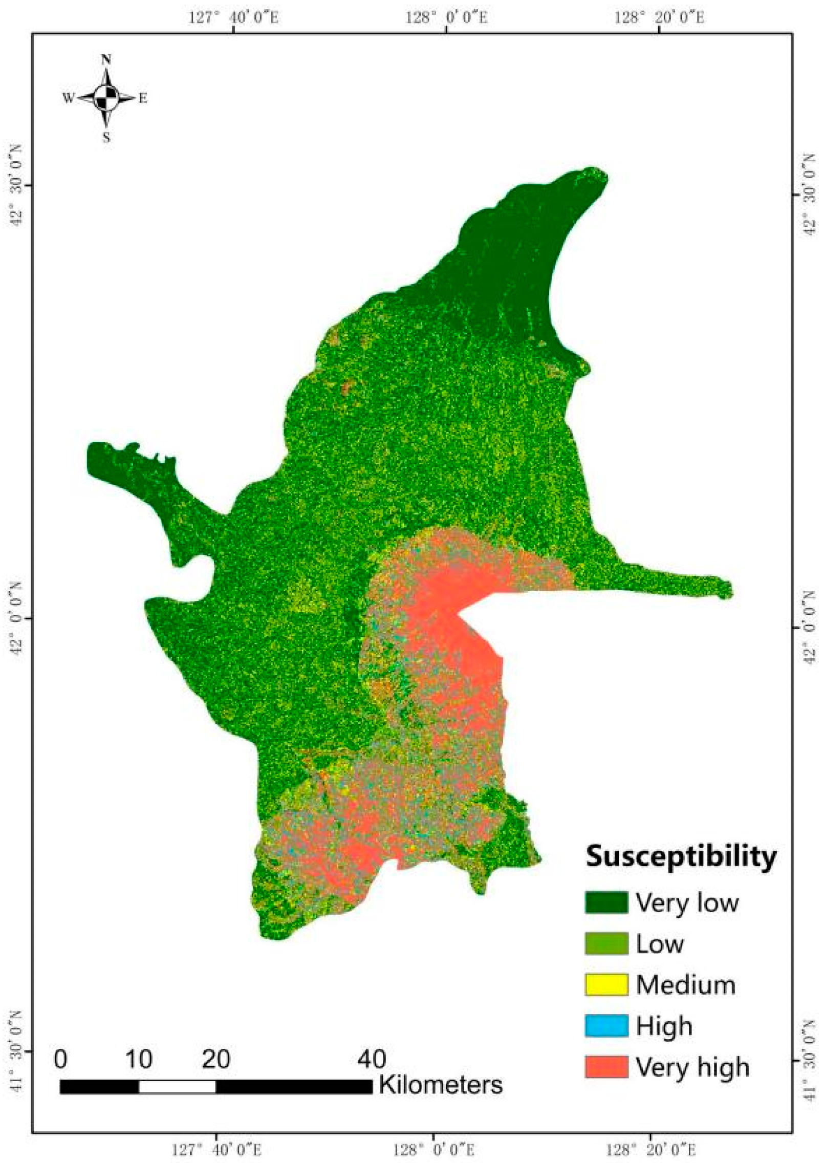
4.2. Susceptibility Assessment Based on CF-SVM
4.3. Earthquake Intensity
5. Risk Assessment
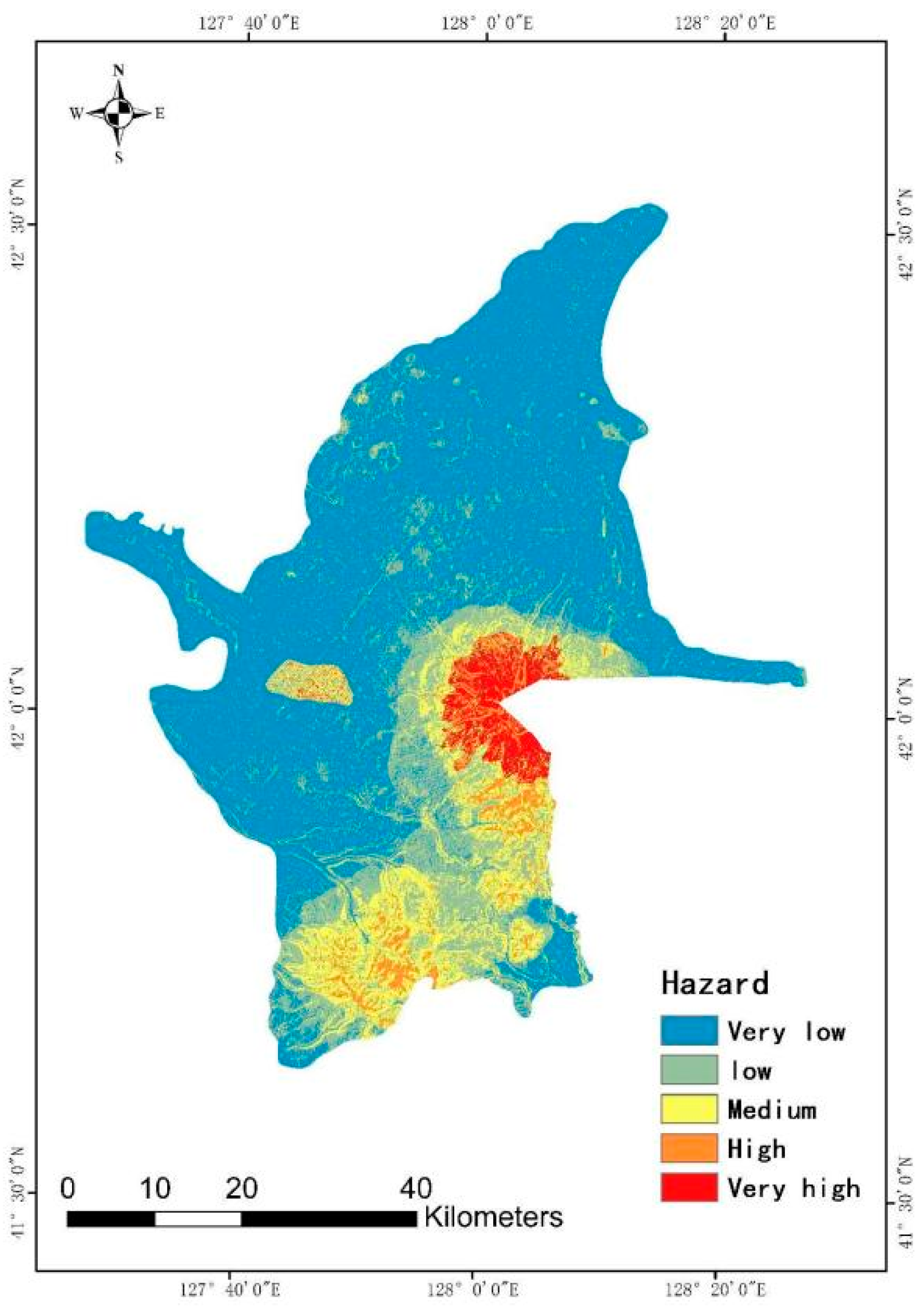
5.1. Hazard Assessment
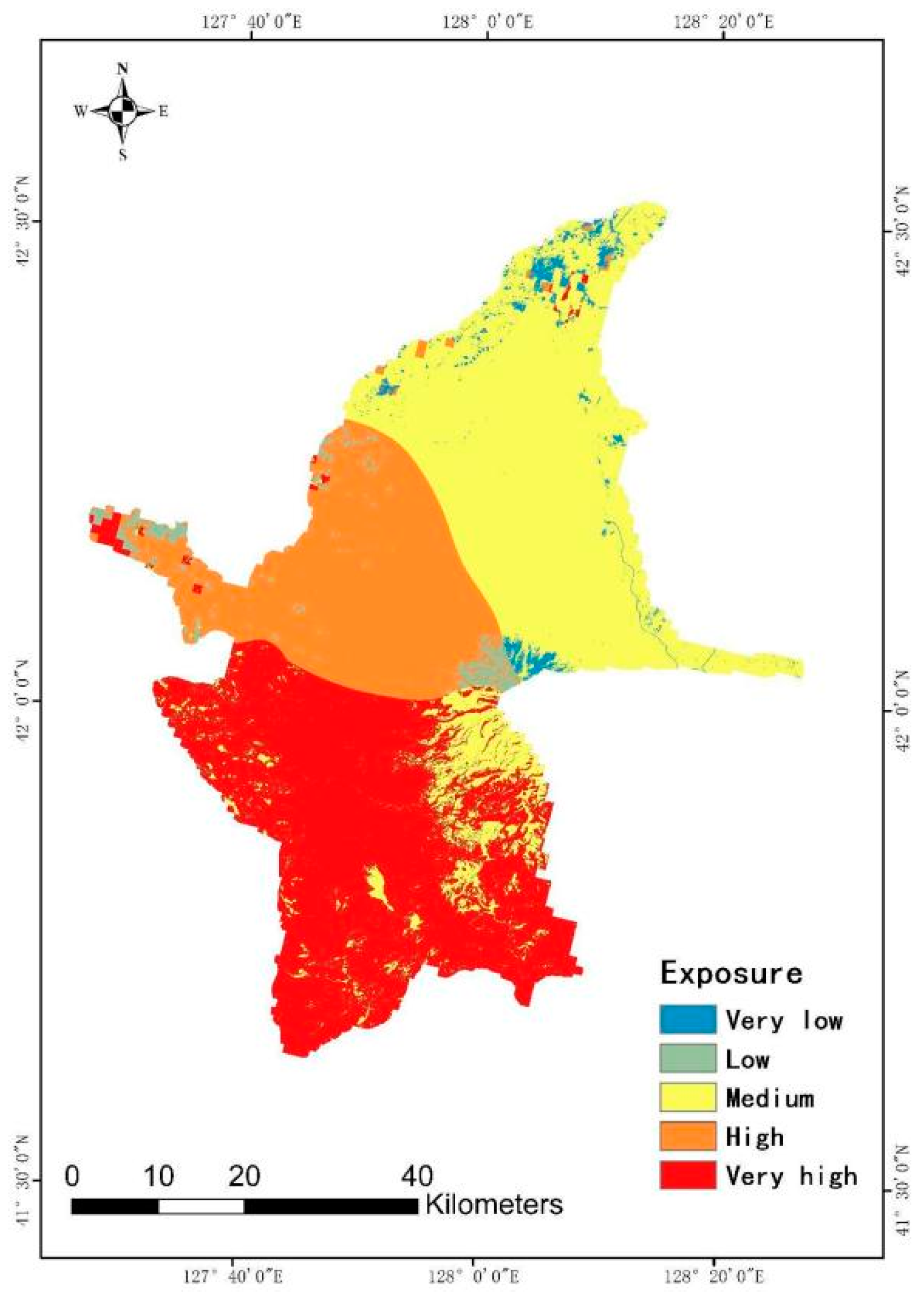
5.2. Carrier Exposure Assessment
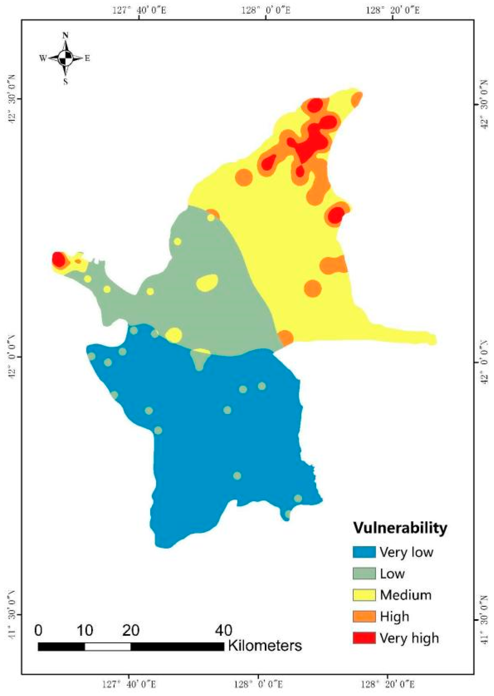
5.3. Carrier Vulnerability Assessment
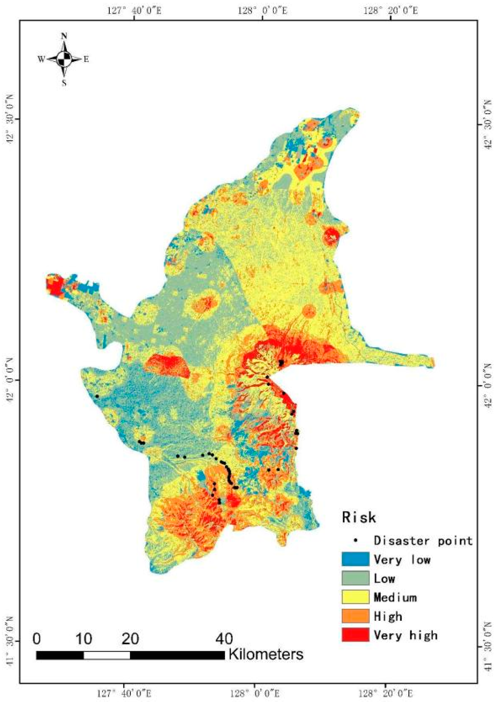
5.4. Results
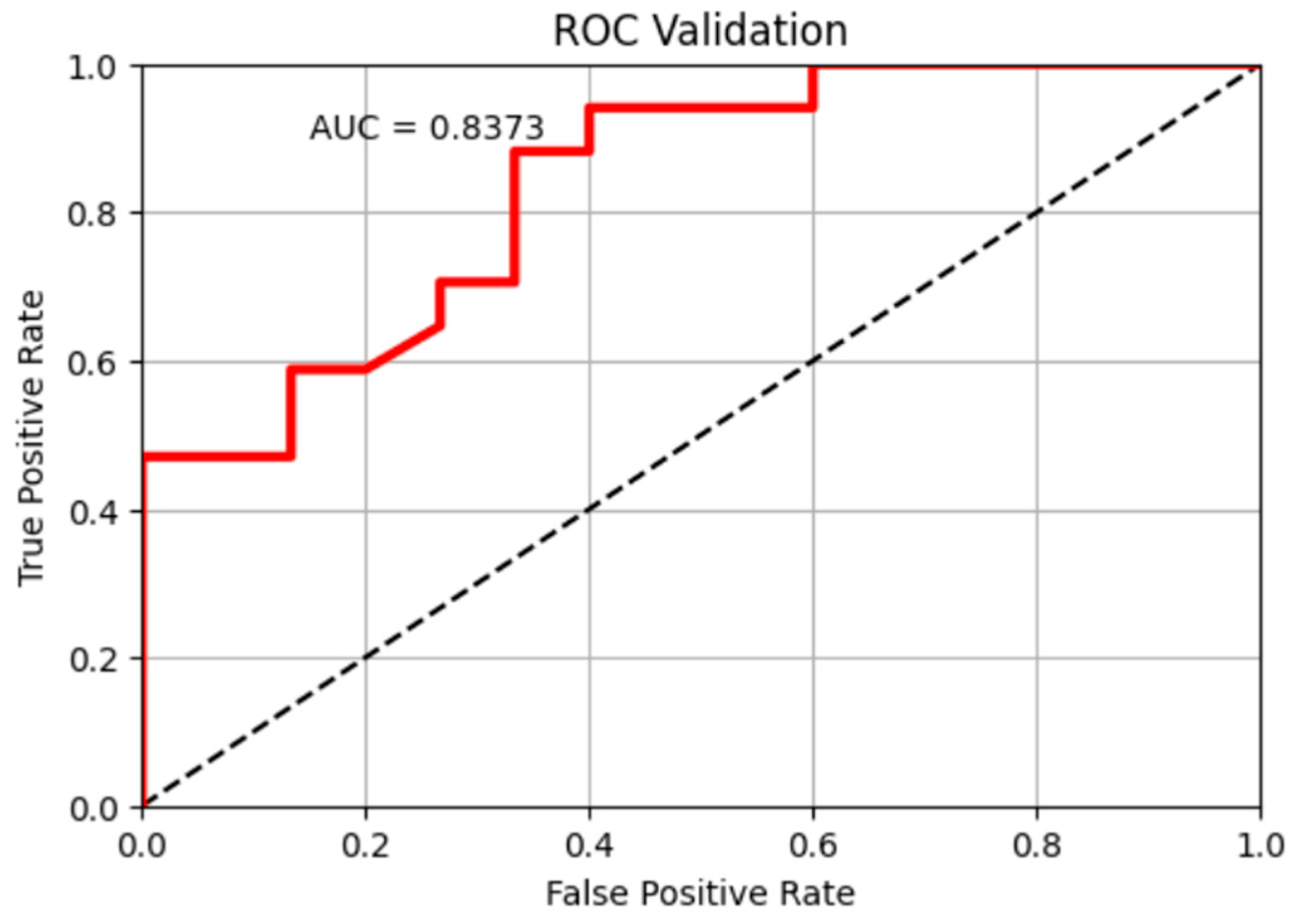
5.5. Result Verification
6. Conclusions
Author Contributions
Funding
Data Availability Statement
Acknowledgments
Conflicts of Interest
References
- Shi, P.J. Theory and practice of disaster study. J. Nat. Disasters 1996, 5, 8–19. [Google Scholar]
- Yin, Y.; Wang, F.; Sun, P. Landslide hazards triggered by the 2008 Wenchuan earthquake, Sichuan, China. Landslides 2009, 6, 139–152. [Google Scholar] [CrossRef]
- Zhang, L.M.; Nadim, F.; Lacasse, S. Multi-risk assessment for landslide hazards. In Proceedings of the Pacific Rim Workshop on Innovations in Civil Infrastructure Engineering, Taipei, Taiwan, 9–11 January 2013; pp. 321–329. [Google Scholar]
- Liu, Z.; Nadim, F.; Garcia-Aristizabal, A.; Mignan, A.; Fleming, K.; Luna, B.Q. A three-level framework for multi-risk assessment. Georisk Assess. Manag. Risk Eng. Syst. Geohazards 2015, 9, 59–74. [Google Scholar] [CrossRef] [Green Version]
- Yin, Y.; Sun, P.; Zhu, J.; Yang, S. Research on catastrophic rock avalanche at Guanling, Guizhou, China. Landslides 2011, 8, 517–525. [Google Scholar] [CrossRef]
- Zhao, L.; Li, D.; Tan, H.; Cheng, X.; Zuo, S. Characteristics of failure area and failure mechanism of a bedding rockslide in Libo County, Guizhou, China. Landslides 2019, 16, 1367–1374. [Google Scholar] [CrossRef]
- Xu, Q.; Fan, X.; Huang, R.; Yin, Y.; Hou, S.; Dong, X.; Tang, M. A catastrophic rockslide-debris flow in Wulong, Chongqing, China in 2009: Background, characterization, and causes. Landslides 2010, 7, 75–87. [Google Scholar] [CrossRef]
- Fan, X.; Xu, Q.; Scaringi, G.; Dai, L.; Li, W.; Dong, X.; Zhu, X.; Pei, X.; Dai, K.; Havenith, H.B. Failure mechanism and kinematics of the deadly June 24th 2017 Xinmo landslide, Maoxian, Sichuan, China. Landslides 2017, 14, 2129–2146. [Google Scholar] [CrossRef]
- Dai, K.; Xu, Q.; Li, Z.; Tomás, R.; Fan, X.; Dong, X.; Li, W.; Zhou, Z.; Gou, J.; Ran, P. Post-disaster assessment of 2017 catastrophic Xinmo landslide (China) by spaceborne SAR interferometry. Landslides 2019, 16, 1189–1199. [Google Scholar] [CrossRef] [Green Version]
- Ouyang, C.; Zhao, W.; Xu, Q.; Peng, D.; Li, W.; Wang, D.; Zhou, S.; Hou, S. Failure mechanisms and characteristics of the 2016 catastrophic rockslide at Su village, Lishui, China. Landslides 2018, 15, 1391–1400. [Google Scholar] [CrossRef]
- Pei, R.R.; Ni, Z.Q.; Meng, Z.B.; Zhang, B.L.; Geng, Y.Y. Cause Analysis of the Secondary Mountain Disaster Chain in Wenchuan Earthquake. Am. J. Civ. Eng. 2017, 5, 414–417. [Google Scholar] [CrossRef]
- Lyu, H.-M.; Shen, J.S.; Arulrajah, A. Assessment of Geohazards and Preventative Countermeasures Using AHP Incorporated with GIS in Lanzhou, China. Sustainability 2018, 10, 304. [Google Scholar] [CrossRef] [Green Version]
- Yang, Z.H.; Lan, H.X.; Gao, X.; Li, L.P.; Meng, Y.S.; Wu, Y.M. Urgent landslide susceptibility assessment in the 2013 Lushan earthquake-impacted area, Sichuan Province, China. Nat. Hazards 2015, 75, 3467–3487. [Google Scholar] [CrossRef]
- Han, L.; Ma, Q.; Zhang, F.; Zhang, Y.; Zhang, J.; Bao, Y.; Zhao, J. Risk Assessment of an Earthquake-Collapse-Landslide Disaster Chain by Bayesian Network and Newmark Models. Int. J. Environ. Res. Public Health 2019, 16, 3330. [Google Scholar] [CrossRef] [Green Version]
- Liu, Y. Typical Debris Flow Disaster Chain Analysis in Tibet Based on RS; Chengdu University of Technology: Chengdu, China, 2013. [Google Scholar]
- He, F.; Tan, S.; Liu, H. Mechanism of rainfall induced landslides in Yunnan Province using multi-scale spatiotemporalanalysis and remote sensing interpretation. Microprocess. Microsyst. 2022, 90, 104502. [Google Scholar] [CrossRef]
- Zhu, L.; He, S.; Qin, H.; He, W.; Zhang, H.; Zhang, Y.; Jian, J.; Li, J.; Su, P. Analyzing the multi-hazard chain induced by a debris flow in Xiaojinchuan River, Sichuan, China. Eng. Geol. 2021, 293, 106280. [Google Scholar] [CrossRef]
- Zhao, Y.; Wang, R.; Jiang, Y.; Liu, H.; Wei, Z. GIS-based logistic regression for rainfall-induced landslide susceptibilitymapping under different grid sizes in Yueqing, Southeastern China. Eng. Geol. 2019, 259, 105147. [Google Scholar] [CrossRef]
- Tian, Y.Y.; Xu, C.; Hong, H.Y.; Zhou, Q.; Wang, D. Mapping earthquake-triggered landslide susceptibility by use of artificial neural network (ANN) models: An example of the 2013 Minxian (China) Mw 5.9 event. Geomat. Nat. Hazards Risk 2019, 10, 1–25. [Google Scholar] [CrossRef] [Green Version]
- Wang, Y.; Song, C.; Lin, Q.; Li, J. Occurrence probability assessment of earthquake-triggered landslides with Newmark displacement values and logistic regression: The Wenchuan earthquake, China. Geomorphology 2016, 258, 108–119. [Google Scholar] [CrossRef]
- Song, Y.; Gong, J.; Gao, S.; Wang, D.; Cui, T.; Li, Y.; Wei, B. Susceptibility assessment of earthquake-induced landslides using Bayesian network: A case study in Beichuan, China. Comput. Geosci. 2012, 42, 189–199. [Google Scholar] [CrossRef]
- Gigović, L.; Pourghasemi, H.R.; Drobnjak, S.; Bai, S. Testing a new ensemble model based on SVM and random forest in forest fire susceptibility assessment and its mapping in Serbia’s Tara National Park. Forests 2019, 10, 408. [Google Scholar] [CrossRef] [Green Version]
- Zhou, W.; Qiu, H.; Wang, L.; Pei, Y.; Tang, B.; Ma, S.; Yang, D.; Cao, M. Combining rainfall-induced shallow landslides and subsequent debris flows for hazard chain prediction. Catena 2022, 213, 106199. [Google Scholar] [CrossRef]
- Fan, X.; Yang, F.; Siva Subramanian, S.; Xu, Q.; Feng, Z.; Mavrouli, O.; Peng, M.; Ouyang, C.; Jansen, J.D.; Huang, R. Prediction of a multi-hazard chain by an integrated numerical simulation approach: The Baige landslide, Jinsha River, China. Landslides 2020, 17, 147–164. [Google Scholar] [CrossRef]
- Ouyang, C.J.; He, S.M.; Tang, C.A. Numerical analysis of dynamics of debris flow over erodible beds in Wenchuan earthquake-induced area. Eng. Geol. 2015, 194, 62–72. [Google Scholar] [CrossRef]
- Ouyang, C.J.; Zhou, K.Q.; Xu, Q.; Yin, J.H.; Peng, D.L.; Wang, D.P.; Li, W.L. Dynamic analysis and numerical modeling of the 2015 catastrophic landslide of the construction waste landfill at Guangming, Shenzhen, China. Landslides 2017, 14, 7015–7718. [Google Scholar] [CrossRef]
- Yi, Z.H. Analysis of Landslide Stability under Earthquake Action; Southwest Jiaotong University: Chengdu, China, 2006. [Google Scholar]
- Jiao, X.E. Analysis of Landslide Stability under Seismic Action; Southwest Jiaotong University: Chengdu, China, 2010. [Google Scholar]
- Cattoni, E.; Salciarini, D.; Tamagnini, C. A Generalized Newmark Method for the assessment of permanent displacements of flexible retaining structures under seismic loading conditions. Soil Dyn. Earthq. Eng. 2019, 117, 221–233. [Google Scholar] [CrossRef]
- Liu, J.M.; Shi, J.S.; Wang, T.; Wu, S.R. Seismic landslide hazard assessment in the Tianshui area, China, based on scenario earthquakes. Bull. Eng. Geol. Environ. 2018, 77, 1263–1272. [Google Scholar] [CrossRef]
- Chousianitis, K.; Del Gaudio, V.; Kalogeras, I.; Ganas, A. Predictive model of Arias intensity and Newmark displacement for regional scale evaluation of earthquake-induced landslide hazard in Greece. Soil Dyn. Earthq. Eng. 2014, 65, 11–29. [Google Scholar] [CrossRef]
- Del Gaudio, V.; Pierri, P.; Calcagnile, G. Analysis of seismic hazard in landslide-prone regions: Criteria and example for an area of Daunia (southern Italy). Nat. Hazards 2012, 61, 203–215. [Google Scholar] [CrossRef]
- Sun, S.; Wang, P.; Yi, J.; Wu, C.; Wang, H.; Chen, H.; Wang, W. Types and distribution of secondary volcanic hazards in Changbaishan Tianchi and adjacent areas and their relationship with volcanic geology. World Geol. 2018, 37, 655–663. [Google Scholar]
- Shortliffe, E.H.; Buchanan, B.G. A model of inexact reasoning in medicine. Math. Biosci. 1975, 23, 351–379. [Google Scholar] [CrossRef]
- Heckerman, D. Probabilistic interpretations for MYCIN’s certainty factors. Mach. Intell. Pattern Recognit. 1986, 4, 167–196. [Google Scholar]
- Polat, A.; Erik, D. Debris flow susceptibility and propagation assessment in West Koyulhisar, Turkey. J. Mt. Sci. 2020, 17, 2611–2623. [Google Scholar] [CrossRef]
- Vapnik, V. The Nature of Statistical Learning Theory; Springer Science & Business Media: Berlin/Heidelberg, Germany, 1999. [Google Scholar]
- Mohammady, M.; Pourghasemi, H.R.; Amiri, M. Assessment of land subsidence susceptibility in Semnan plain (Iran): A comparison of support vector machine and weights of evidence data mining algorithms. Nat. Hazards 2019, 99, 951–971. [Google Scholar] [CrossRef]
- Cherkassky, V. The nature of statistical learning theory. IEEE Trans. Neural Netw. 1997, 8, 1564. [Google Scholar] [CrossRef] [Green Version]
- Tehrany, M.S.; Pradhan, B.; Mansor, S.; Ahmad, N. Flood susceptibility assessment using GIS-based support vector machine model with different kernel types. Catena 2015, 125, 91–101. [Google Scholar] [CrossRef]
- Wang, H.Y.; Lai, J.F.; Yang, F.L. A review of support vector machine theory and algorithm research. Comput. Appl. Res. 2014, 31, 1281–1286. [Google Scholar]
- Li, Y.; Mei, H.; Ren, X.; Hu, X.; Li, M. Evaluation of geological disaster susceptibility based on deterministic coefficient and support vector machine. J. Earth Inf. Sci. 2018, 20, 1699–1709. [Google Scholar]
- Xue, Y.; Wang, Y.; Zhu, J.; Li, H.; Zhang, M. Study on sensitivity assessment of geological slope based on CF and SVM. J. Taiyuan Univ. Technol. 2022, 53, 672–681. [Google Scholar] [CrossRef]
- Wang, T. Research on Geological Hazard Assessment in the Hardest Hit Areas of Wenchuan Earthquake; China Academy of Geological Sciences: Beijing, China, 2010. [Google Scholar]
- Jibson, R.W. Regression models for estimating coseismic landslide displacement. Eng. Geol. 2007, 91, 209–218. [Google Scholar] [CrossRef]
- Wilson, R. Predicting areal limit of earthquake-induced landsliding, evaluating eathquake hazards in the Los Angeles region-an earth-science perspective. US Geol. Survery Prof. Pap. 1985, 1360, 317–345. [Google Scholar]
- Ding, B.; Sun, J.; Li, X.; Liu, Z.; Du, J. Research progress and discussion of the correlation between seismic intensity and ground motion parameters. J. Earthq. Eng. Eng. Vib. 2014, 34, 7–20. [Google Scholar]
- Newmark, N.M. Effects of Earthquakes on Dams and Embankments. Géotechnique 1965, 15, 139–160. [Google Scholar] [CrossRef] [Green Version]
- Du, Y.; Ge, Y.; Liang, X.; Sun, Q.; Chen, P. Study on the assessment method of the deterministic coefficient and geodetector model—Take the Anning River basin as an example. J. Disaster Prev. Mitig. Eng. 2022, 42, 664–673. [Google Scholar] [CrossRef]
- Li, W.; Hong, T.; Xu, S.; Chen, M.; Qin, Y.; Zeng, L. Evaluation of geological disaster susceptibility in Rongjiang County based on I method and CF method. Geol. Disaster Environ. Prot. 2022, 33, 42–48. [Google Scholar]
- Smith, R.; Kilburn, C.R.J. Forecasting eruptions after long repose intervals from accelerating rates of rock fracture: The June 1991 eruption of Mount Pinatubo, Philippines. J. Volcanol. Geotherm. Res. 2010, 191, 129–136. [Google Scholar] [CrossRef]
- Swets, J.A. Measuring the accuracy of diagnostic systems. Science 1988, 240, 1285–1293. [Google Scholar] [CrossRef] [Green Version]
- Fawcett, T. An introduction to ROC analysis. Pattern Recognit. Lett. 2006, 27, 861–874. [Google Scholar] [CrossRef]
- Lei, Z.; Li, L.; Long, J.; Chen, J.; Yang, Y. Improvement of Newmark model based on rainfallinfiltration and prediction of seismic landslide hazard. J. Earthq. Eng. 2022, 44, 527–534. [Google Scholar] [CrossRef]
- Zhao, N.; Ma, F.S.; Li, C.Q.; Guo, J.; Zhang, J.C. Optimization and application of parameters of probabilistic seismic landslide hazard model based on Newmark model: An example in Ludian seismic zone. Earth Sci. 2022, 47, 4401–4416. [Google Scholar]


| Evaluation Index | Data Type | Resolution | Data Source |
|---|---|---|---|
| Elevation | raster data | 30 m | Geospatial data cloud |
| Land use type | raster data | 30 m | National Center for Basic Geographic Information |
| Rainfall | raster data | 30 m | National Data Center for Meteorological Sciences |
| Fractional vegetation cover | Landsat 8 OLI/TIRS | 30 m | Satellite remote sensing cloud for natural resources |
| Slope | raster data | 30 m | Geospatial data cloud |
| Distance to river | vector data | 30 m | Geospatial data cloud |
| Aspect | raster data | 30 m | Geospatial data cloud |
| Lithology | vector data | 30 m | Geological cloud |
| Relief intensity | vector data | 30 m | Geospatial data cloud |
| Topographic wetness index | vector data | 30 m | Resources and Environmental Sciences and Data Center, Chinese Academy of Sciences |
| Earthquake intensity | raster data | 30 m | Google earth pro |
| Terrain roughness | vector data | 30 m | Resources and Environmental Sciences and Data Center, Chinese Academy of Sciences |
| Population | vector data | 30 m | Resources and Environmental Sciences and Data Center, Chinese Academy of Sciences |
| Gross national product | vector data | 30 m | Resources and Environmental Sciences and Data Center, Chinese Academy of Sciences |
| Building density | vector data | 30 m | National Center for Basic Geographic Information |
| Road density | vector data | 30 m | National Center for Basic Geographic Information |
| Age level | vector data | 30 m | Resources and Environmental Sciences and Data Center, Chinese Academy of Sciences |
| Rock Group | c/ | /(°) | |
|---|---|---|---|
| Hard rock | >0.22 | >37 | >26.5 |
| Second hard rock | 0.12–0.22 | 29–37 | >26.5 |
| Second soft rock | 0.08–0.12 | 19–29 | 24.5–26.5 |
| Evaluation Index | Grade | Grading Area Ratio | Disaster Point Ratio | CF | Frequency Ratio | ||
|---|---|---|---|---|---|---|---|
| Slope/(°) | 0–5 | 0.5677 | 0.2692 | 0.0075 | 0.0073 | −0.5297 | 0.4742 |
| 5–10 | 0.2531 | 0.1923 | 0.0120 | 0.0118 | −0.2432 | 0.7596 | |
| 10–15 | 0.0758 | 0.0769 | 0.0160 | — | 0.0145 | 1.0144 | |
| 15–25 | 0.0695 | 0.2115 | 0.0481 | — | 0.6820 | 3.0420 | |
| 25–65 | 0.0337 | 0.25 | 0.1173 | — | 0.8789 | 7.4085 | |
| aspect/(°) | −1–0 | 0.1142 | 0.0576 | 0.0079 | 0.0157 | −0.4990 | 0.5049 |
| 0–22.5 | 0.1043 | 0.0961 | 0.0145 | 0.0156 | −0.0799 | 0.9211 | |
| 22.5–67.5 | 0.0854 | 0.0961 | 0.0178 | — | 0.1131 | 1.1253 | |
| 67.5–112.5 | 0.0680 | 0.0192 | 0.0044 | 0.0157 | −0.7204 | 0.2827 | |
| 112.5–157.5 | 0.0655 | 0 | 0 | 0.0158 | −1 | 0 | |
| 157.5–202.5 | 0.0942 | 0.0192 | 0.0032 | 0.0157 | −0.7986 | 0.2039 | |
| 202.5–247.5 | 0.1108 | 0.1730 | 0.0247 | — | 0.3653 | 1.5614 | |
| 247.5–292.5 | 0.1205 | 0.1730 | 0.0227 | — | 0.3081 | 1.4353 | |
| 292.5–337.5 | 0.1189 | 0.1730 | 0.0230 | — | 0.3180 | 1.4556 | |
| 337.5–360.0 | 0.1177 | 0.1923 | 0.0258 | — | 0.3938 | 1.6329 | |
| Topographic wetness index (TWI) | 2.8–6 | 0.1415 | 0.2692 | 0.0301 | — | 0.4819 | 1.9022 |
| 6–8 | 0.5565 | 0.4807 | 0.0136 | 0.0156 | −0.1380 | 0.8638 | |
| 8–10 | 0.1632 | 0.1538 | 0.0149 | 0.0156 | −0.0584 | 0.9424 | |
| 10–15 | 0.1205 | 0.0961 | 0.0126 | 0.0156 | −0.2050 | 0.7975 | |
| 15–24 | 0.0181 | 0 | 0 | 0.0158 | −1 | 0 | |
| Fractional vegetation cover (FVC) | 0.0–0.2 | 0.0638 | 0.1923 | 0.0475 | — | 0.6774 | 3.0106 |
| 0.2–0.5 | 0.0273 | 0.0769 | 0.0443 | — | 0.6534 | 2.8109 | |
| 0.5–0.8 | 0.2822 | 0.2307 | 0.0129 | 0.0156 | −0.1874 | 0.8176 | |
| 0.8–0.9 | 0.3090 | 0.2884 | 0.0147 | 0.0156 | −0.0708 | 0.9332 | |
| 0.9–1.0 | 0.3174 | 0.2115 | 0.0105 | 0.0156 | −0.3393 | 0.6664 | |
| Rainfall/(mm) | <7000 | 0.0840 | 0 | 0 | 0.012456035 | −1 | 0 |
| 7000–8000 | 0.6276 | 0.1923 | 0.0038 | 0.012408498 | −0.6962 | 0.3063 | |
| 8000–9000 | 0.2461 | 0.5384 | 0.0272 | — | 0.5497 | 2.1879 | |
| 9000–10000 | 0.0387 | 0.2115 | 0.0680 | — | 0.8272 | 5.4625 | |
| >10000 | 0.0034 | 0.0576 | 0.2069 | — | 0.9516 | 16.6164 | |
| Land use type | Cultivated land | 0.0139 | 0 | 0 | 0.0158 | −1 | 0 |
| Wood land | 0.8906 | 0.8269 | 0.0146 | 0.0156 | −0.0755 | 0.9284 | |
| Grass land | 0.0757 | 0.0961 | 0.0200 | — | 0.2128 | 1.2690 | |
| Waters | 0.0017 | 0 | 0 | 0.0158 | −1 | 0 | |
| Construction land | 0.0145 | 0 | 0 | 0.0158 | −1 | 0 | |
| Snow cover | 0.0033 | 0.0769 | 0.3637 | — | 0.9718 | 23.0417 | |
| Lithology | Basalt | 0.7952 | 0.6538 | 0.0129 | 0.0156 | −0.1828 | 0.8221 |
| Glutenite | 0.1336 | 0.0769 | 0.0090 | 0.0156 | −0.4300 | 0.5757 | |
| Trachyte | 0.0552 | 0.25 | 0.0714 | — | 0.7907 | 4.5235 | |
| Granite | 0.0158 | 0.0192 | 0.0191 | — | 0.1765 | 1.2141 | |
| Earthquake intensity | Ⅶ | 0.1871 | 0.3269 | 0.0275 | — | 0.4326 | 1.7472 |
| Ⅵ | 0.6868 | 0.6730 | 0.0154 | 0.0155 | −0.0236 | 0.9798 | |
| Ⅴ | 0.1260 | 0 | 0 | 0.0158 | −1 | 0 | |
| Distance to river/(m) | <500 | 0.0461 | 0.0192 | 0.0071 | 0.0168 | −0.5878 | 0.4162 |
| 500–1000 | 0.0473 | 0 | 0 | 0.0169 | −1 | 0 | |
| 1000–1500 | 0.0488 | 0.0192 | 0.0066 | 0.0168 | −0.6101 | 0.3939 | |
| 1500–2000 | 0.0499 | 0.0192 | 0.0065 | 0.0168 | −0.6189 | 0.3851 | |
| >2000 | 0.8076 | 0.9423 | 0.0197 | — | 0.1453 | 1.1666 | |
| Terrain roughness | <10 | 0.3686 | 0.7115 | 0.0306 | — | 0.4896 | 1.9298 |
| 10–25 | 0.4202 | 0.2692 | 0.0101 | 0.0157 | −0.3630 | 0.6406 | |
| 25–45 | 0.1399 | 0 | 0 | 0.0159 | −1 | 0 | |
| 45–100 | 0.0586 | 0.0192 | 0.0052 | 0.0158 | −0.675 | 0.3277 | |
| >100 | 0.0124 | 0 | 0 | 0.0159 | −1 | 0 |
| Model | Susceptibility | Division Area/km2 | Area Proportion/% | Disaster Point | Disaster Point Ratio/% | Fr |
|---|---|---|---|---|---|---|
| CF-SVM | Very low | 1505.52 | 45.85 | 4 | 7.69 | 0.17 |
| Low | 685.73 | 20.88 | 6 | 11.54 | 0.55 | |
| Moderation | 419.76 | 12.78 | 4 | 7.69 | 0.60 | |
| High | 175.21 | 5.34 | 6 | 11.54 | 2.16 | |
| Very high | 497.23 | 15.15 | 32 | 61.54 | 4.06 |
| Primary Factor | Index | Weight Coefficient |
|---|---|---|
| Demographic factor | population | 0.2272 |
| Ecological environment factors | land use type | 0.2421 |
| Socioeconomic factor | gross national product | 0.5307 |
| Primary Factor | Index | Weight Coefficient |
|---|---|---|
| Demographic factor | Building density | 0.4856 |
| Ecological environment factors | Road density | 0.1690 |
| Socioeconomic factor | Age level | 0.3454 |
Disclaimer/Publisher’s Note: The statements, opinions and data contained in all publications are solely those of the individual author(s) and contributor(s) and not of MDPI and/or the editor(s). MDPI and/or the editor(s) disclaim responsibility for any injury to people or property resulting from any ideas, methods, instructions or products referred to in the content. |
© 2023 by the authors. Licensee MDPI, Basel, Switzerland. This article is an open access article distributed under the terms and conditions of the Creative Commons Attribution (CC BY) license (https://creativecommons.org/licenses/by/4.0/).
Share and Cite
Ke, K.; Zhang, Y.; Zhang, J.; Chen, Y.; Wu, C.; Nie, Z.; Wu, J. Risk Assessment of Earthquake–Landslide Hazard Chain Based on CF-SVM and Newmark Model—Using Changbai Mountain as an Example. Land 2023, 12, 696. https://doi.org/10.3390/land12030696
Ke K, Zhang Y, Zhang J, Chen Y, Wu C, Nie Z, Wu J. Risk Assessment of Earthquake–Landslide Hazard Chain Based on CF-SVM and Newmark Model—Using Changbai Mountain as an Example. Land. 2023; 12(3):696. https://doi.org/10.3390/land12030696
Chicago/Turabian StyleKe, Kai, Yichen Zhang, Jiquan Zhang, Yanan Chen, Chenyang Wu, Zuoquan Nie, and Junnan Wu. 2023. "Risk Assessment of Earthquake–Landslide Hazard Chain Based on CF-SVM and Newmark Model—Using Changbai Mountain as an Example" Land 12, no. 3: 696. https://doi.org/10.3390/land12030696