
Assessing Integrated Hydrologic Model: From Benchmarking to Case Study in a Typical Arid and Semi-Arid Basin


Abstract
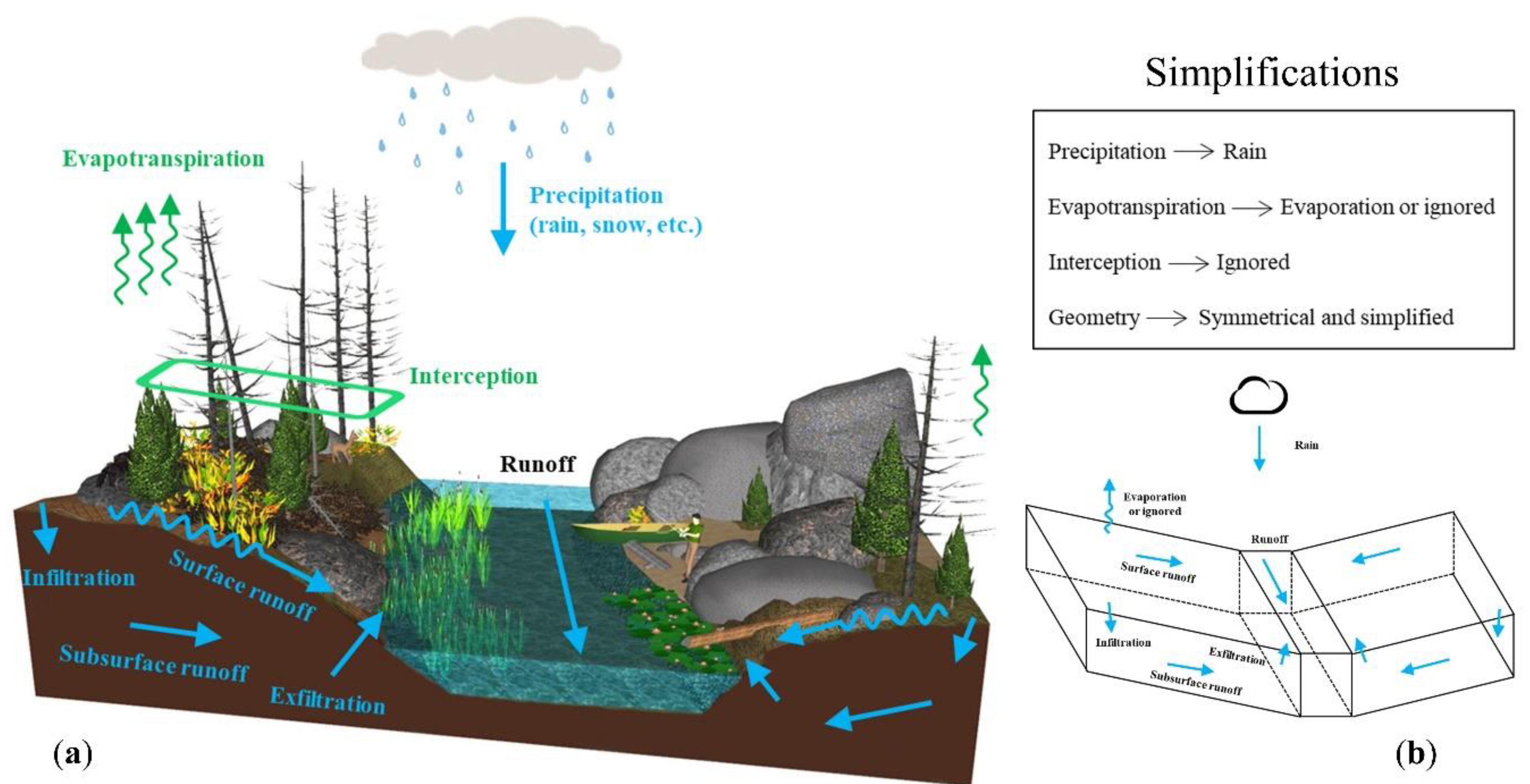
:1. Introduction
2. Methodology
2.1. Integrated Hydrologic Model: ParFlow
2.2. Benchmarking Case Descriptions
2.2.1. Assessment Methodology
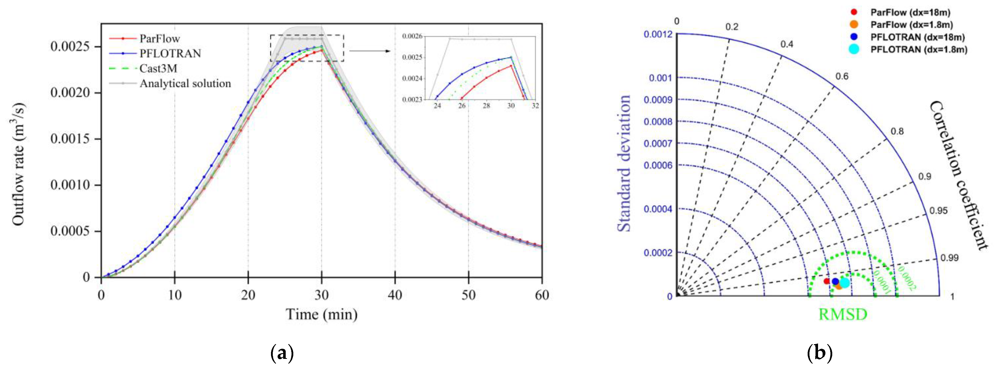
2.2.2. Benchmarking Case 1: 1D Parking Lot Case
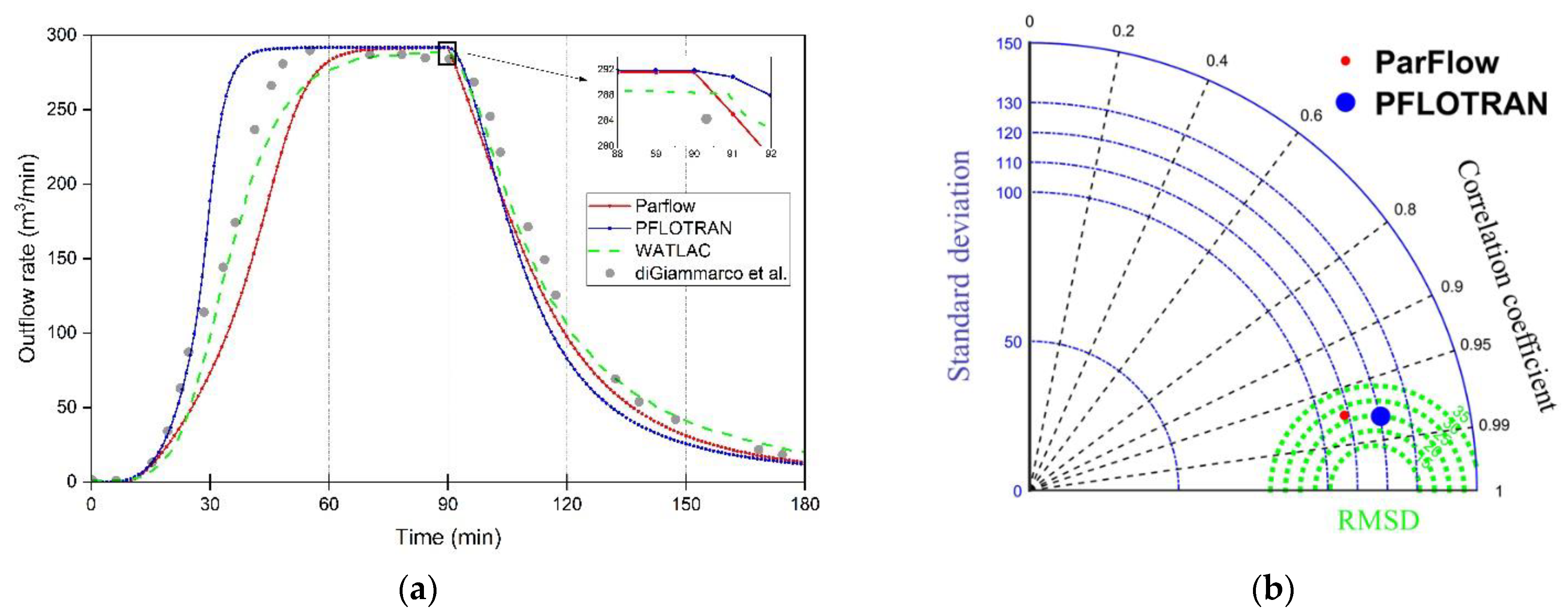
2.2.3. Benchmarking Case 2: 2D Tilted V-Catchment Case
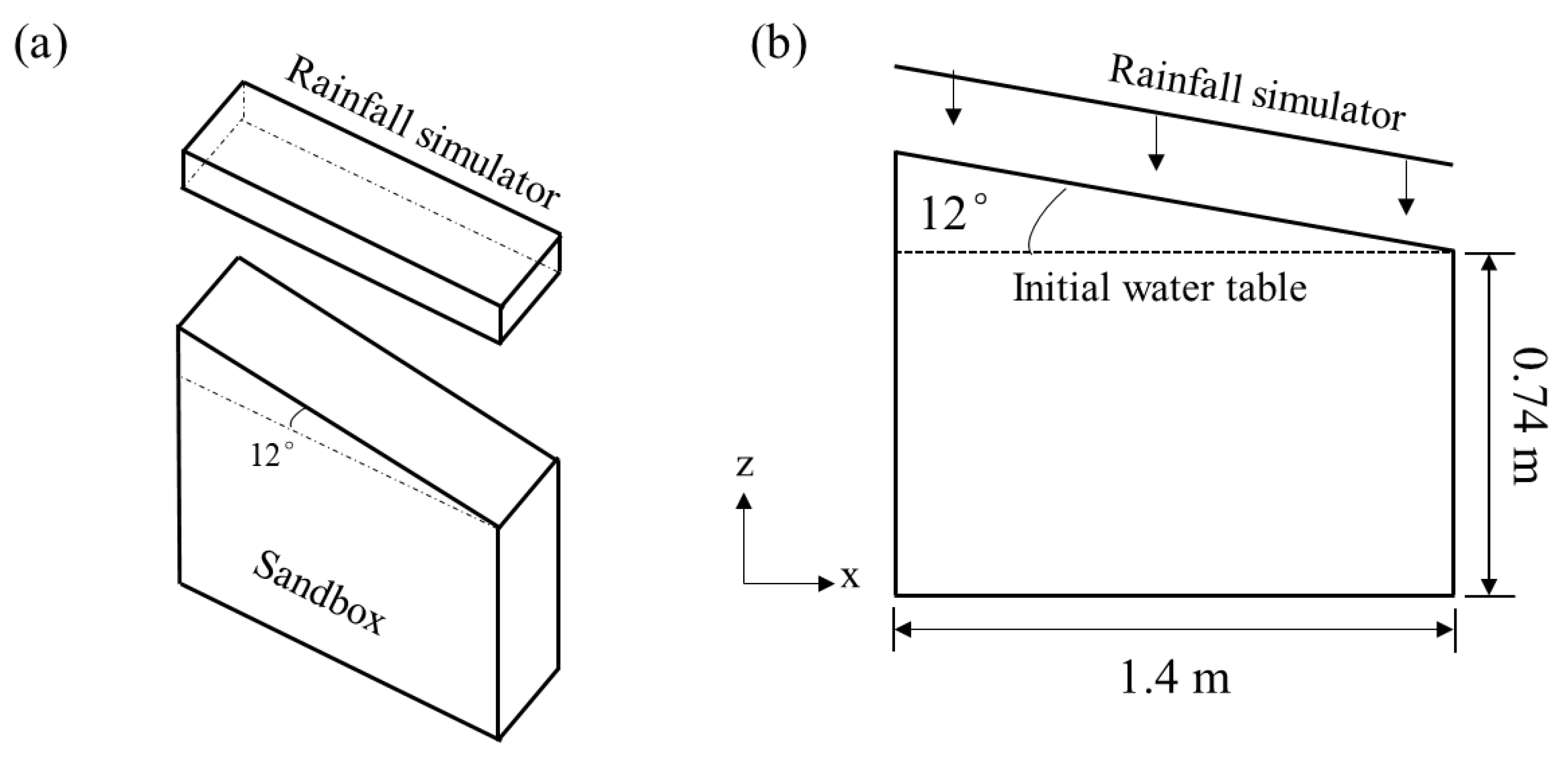
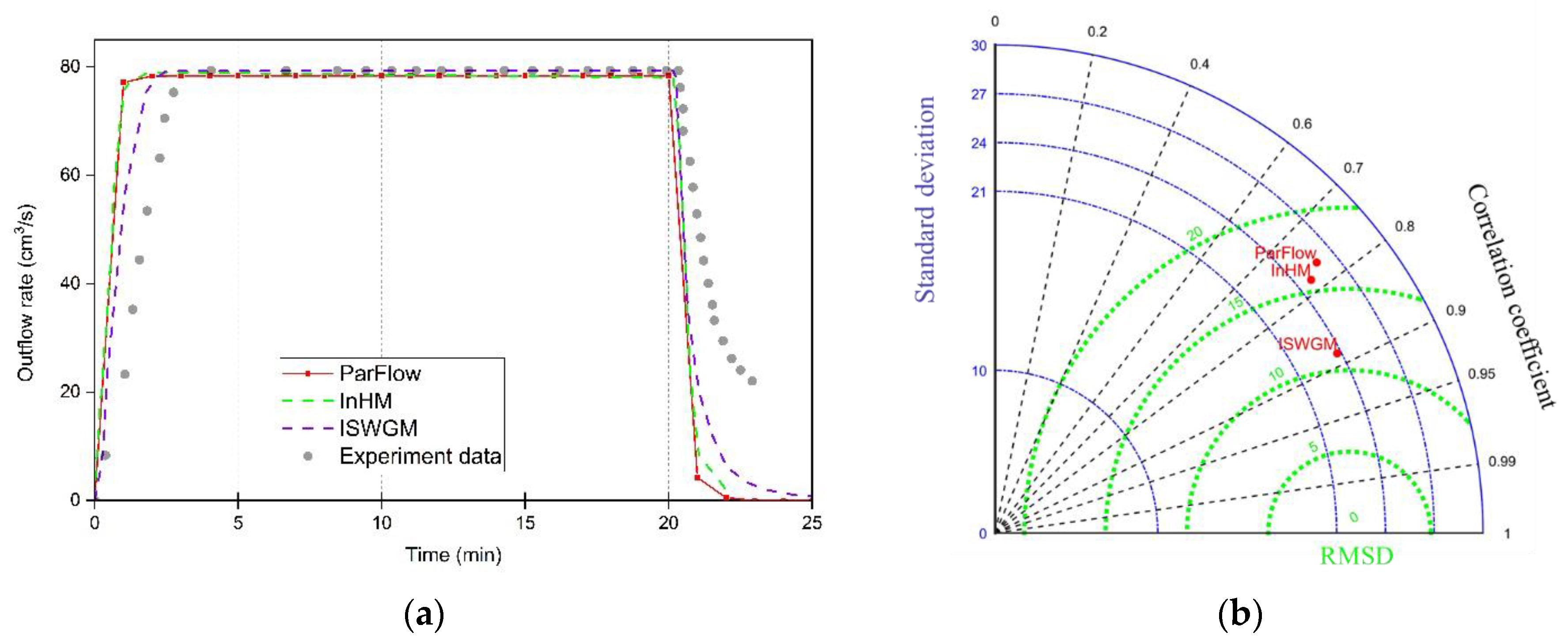
2.2.4. Benchmarking Case 3: Integrated Groundwater-Surface Water Flow
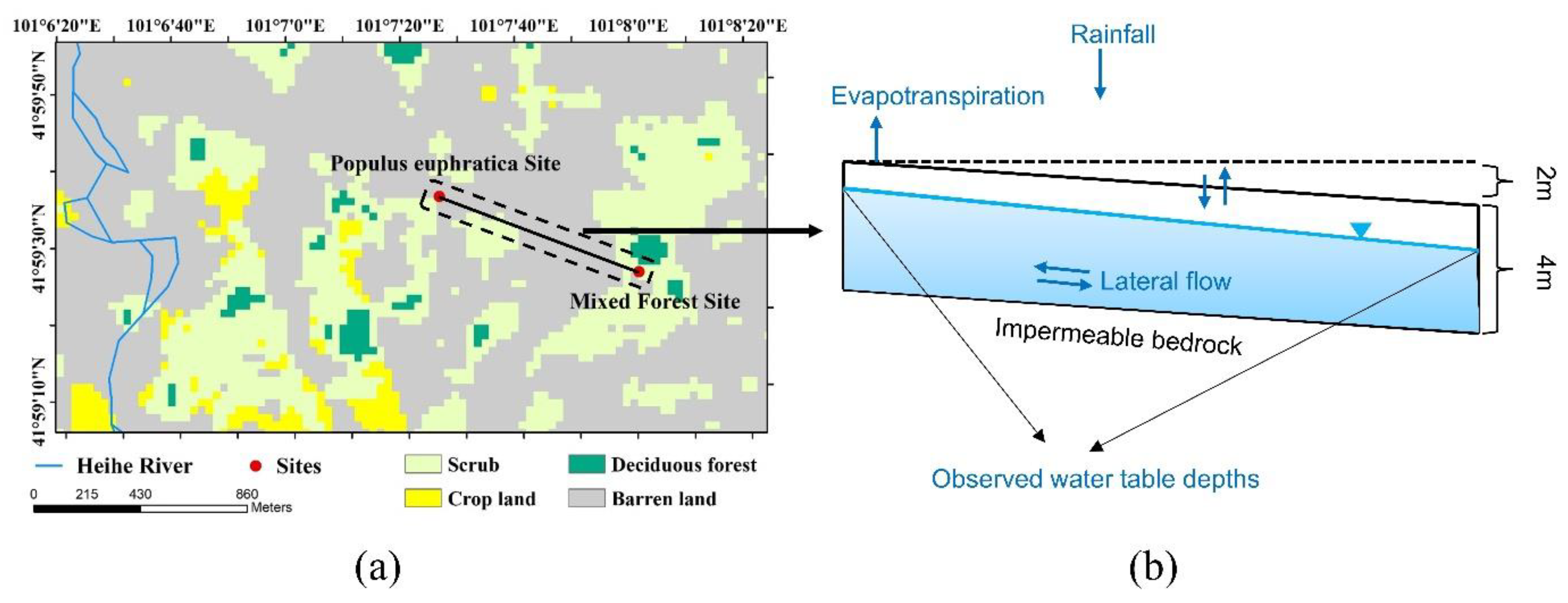
2.3. Validation Case: The Bajajihu (BJH) Case
2.3.1. Modeling Domain
2.3.2. Model Setup
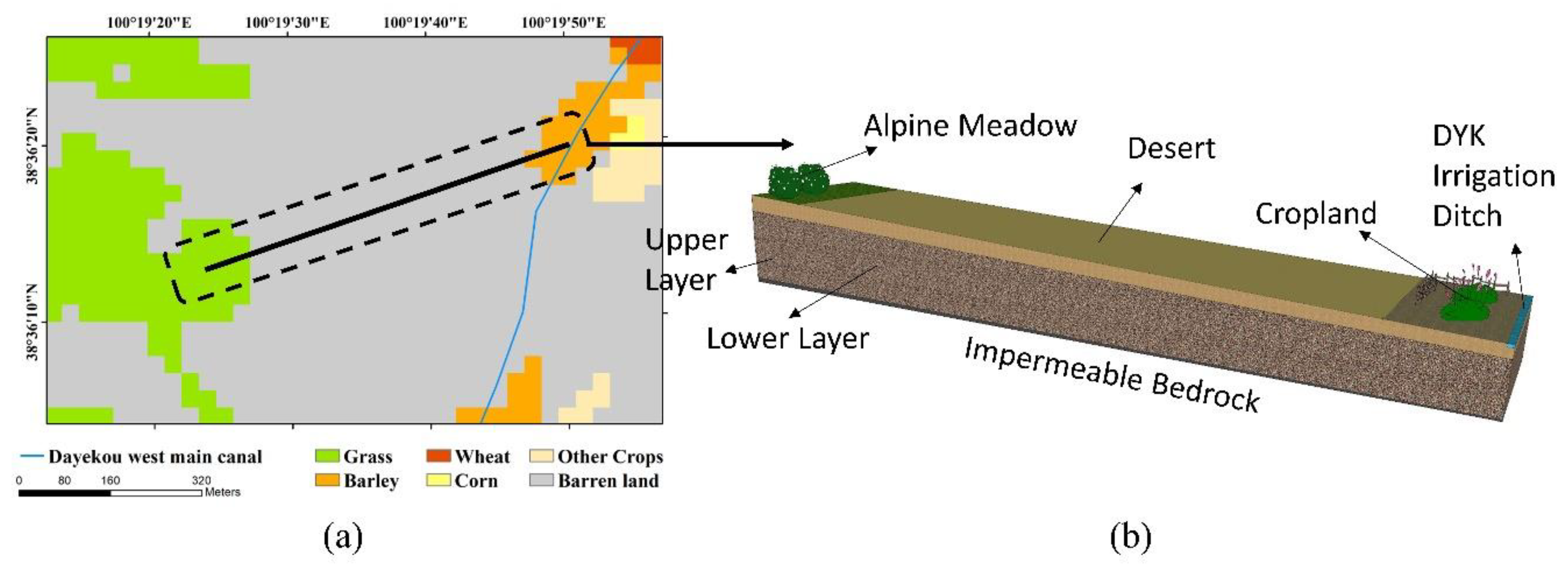
2.4. Application Case: The Dayekou (DYK) Case
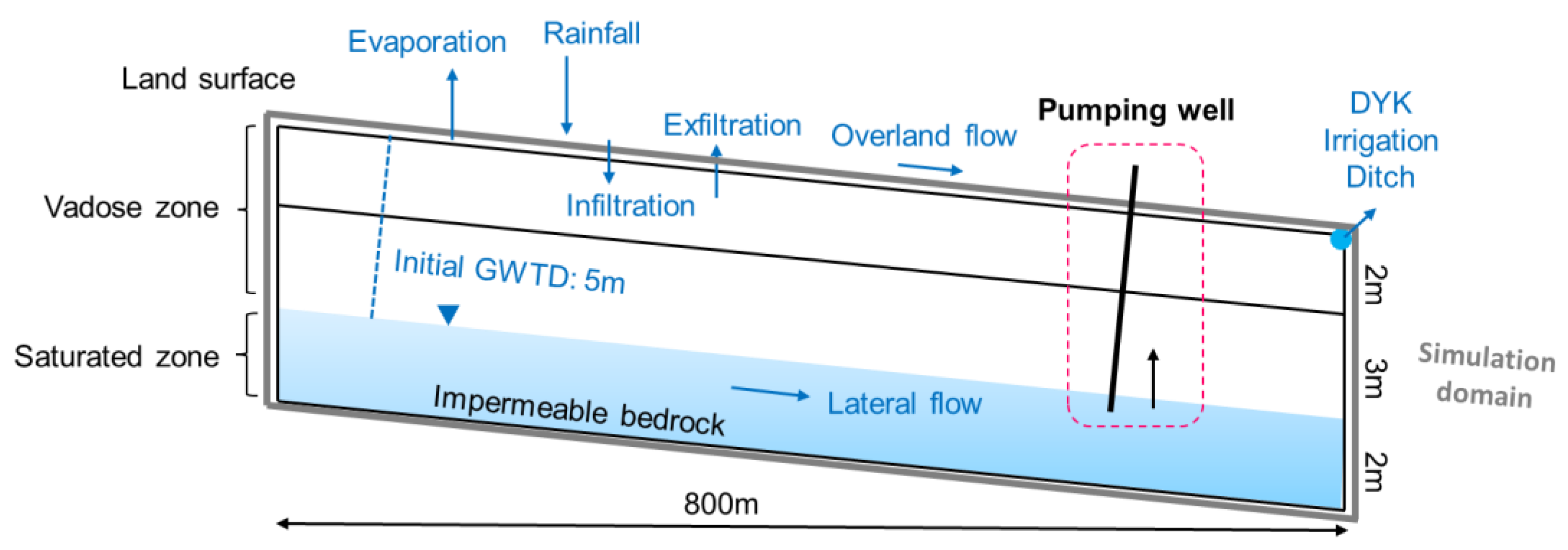
2.4.1. Modeling Domain
2.4.2. Model Setup
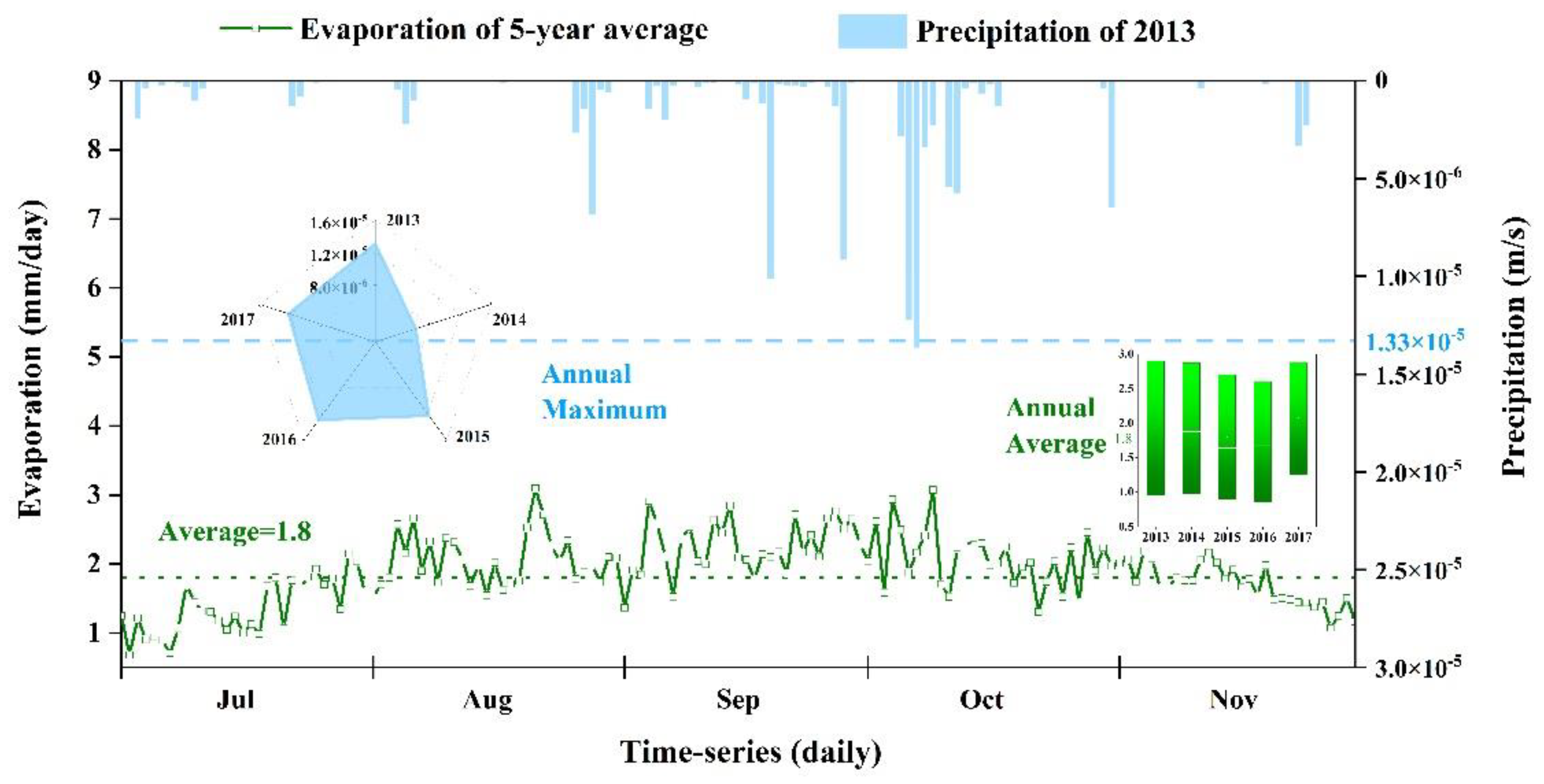
2.4.3. Forcing Data
2.4.4. Scenarios
3. Results and Discussion
3.1. Benchmarking Case 1: 1D Parking Lot Case
3.2. Benchmarking Case 2: 2D Tilted V-Catchment Case
3.3. Benchmarking Case 3: Integrated Groundwater-Surface Water Flow
3.4. Benchmarking Assessment Summary
4. Case Studies in the Heihe River Basin
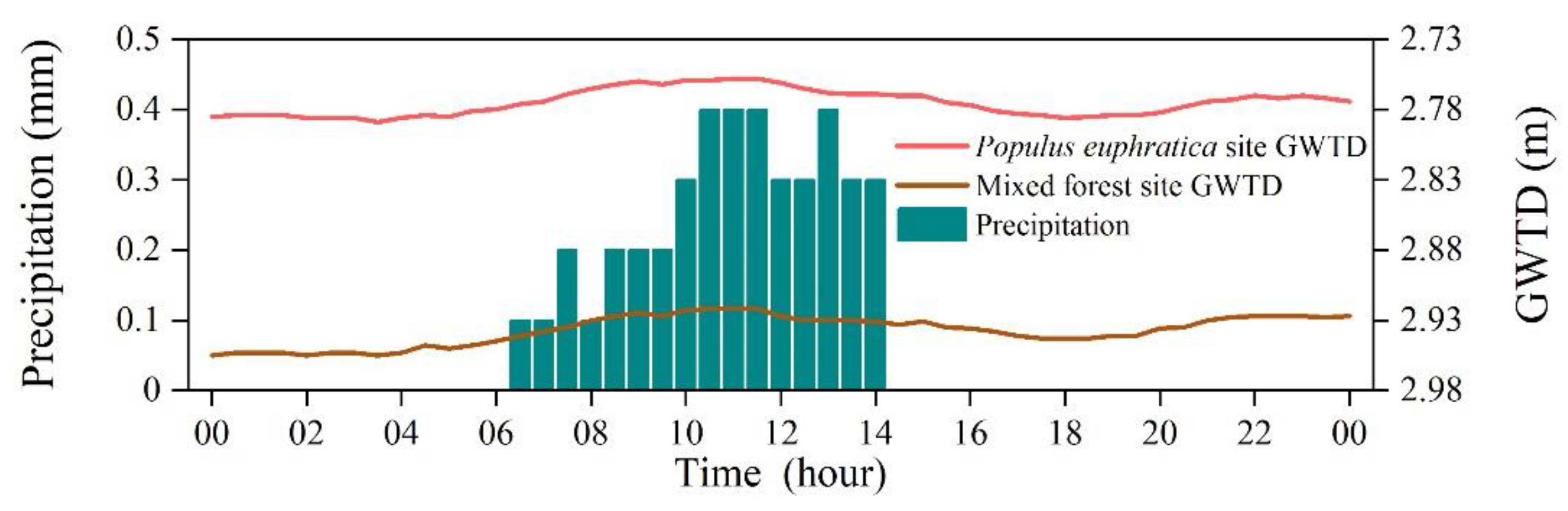
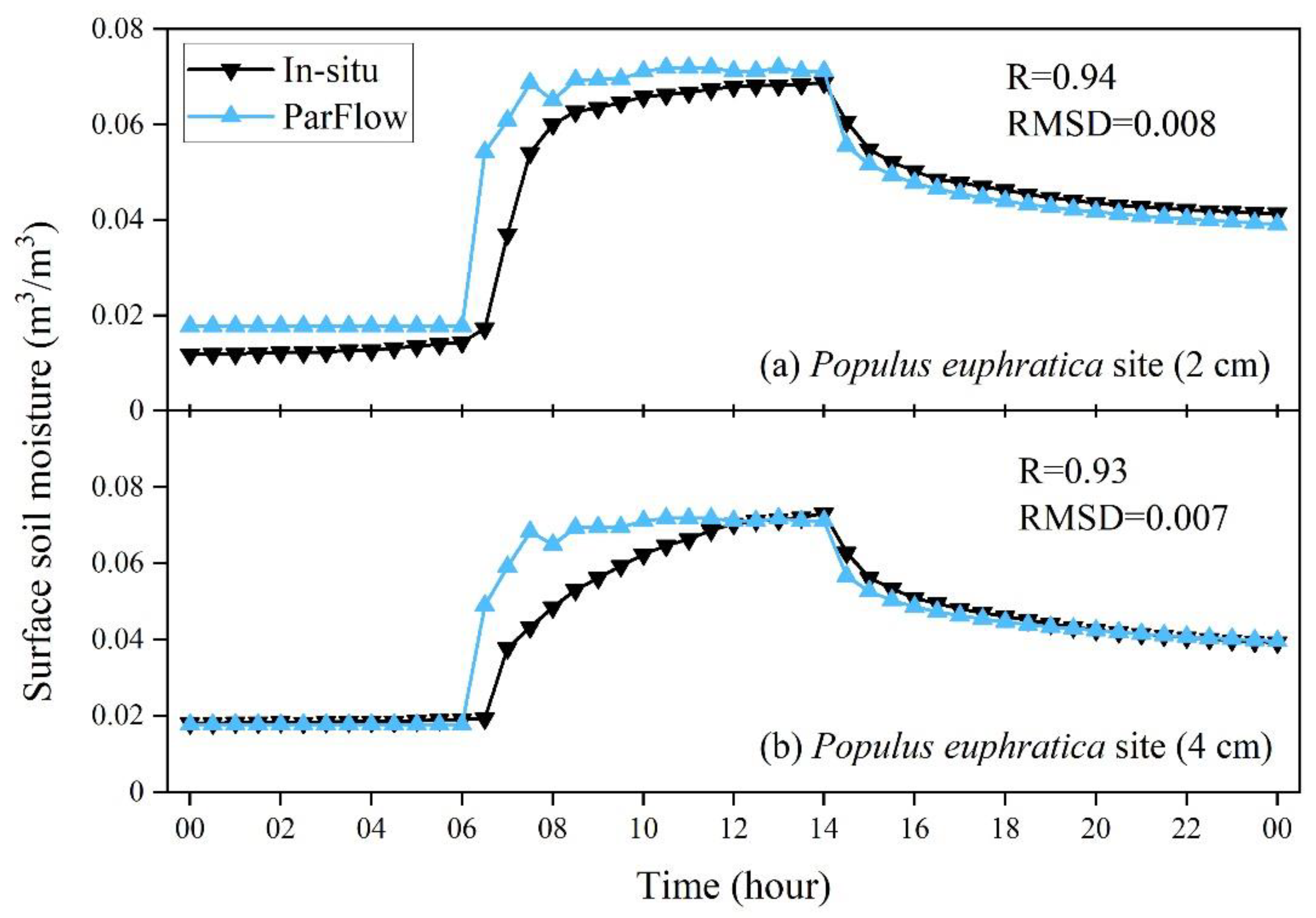
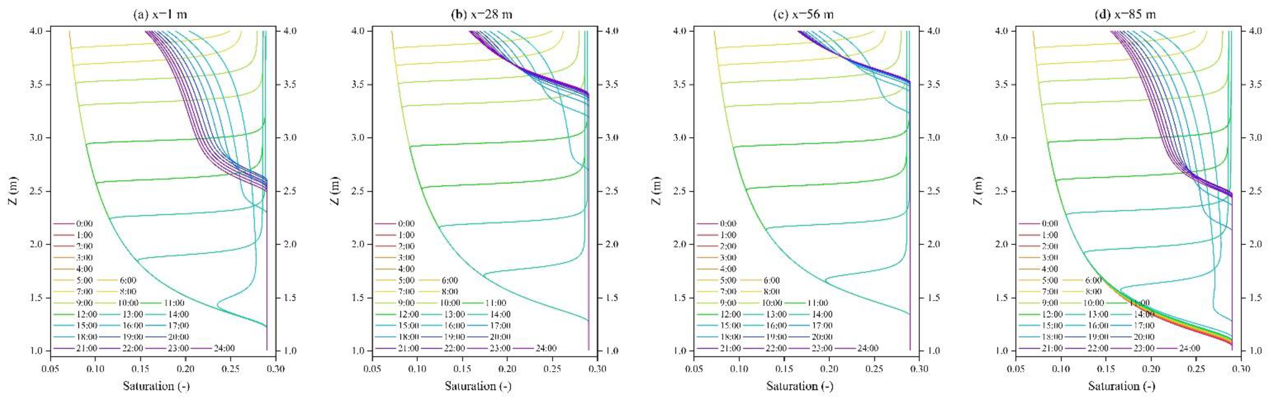
4.1. Results and Analyses of Validation Case: The Bajajihu (BJH) Case
4.2. Results and Analyses of Application Case: The Dayekou (DYK) Case
5. Conclusions
- Benchmarking cases are summarized and categorized progressively from simplicity to complexity. The benchmarking cases cover a nearly full range of typical benchmarking cases to diagnose hydrologic responses, which enables subsequent users to build confidence. In each case, selected references are involved in validating results simulated by ParFlow. Generally, ParFlow can simulate the hydrological response for overland flow and integrated groundwater-surface water systems.
- An overall performance assessment of corresponding hydrologic signals is explored and applied using modified Taylor diagrams, which demonstrates ParFlow’s capability of quantifying integrated hydrologic cycles with high efficiency. It can improve understanding of evaluation methodology and enhance the quantitative analysis of groundwater-surface water modeling.
- A 2D transect is configured in the BJH, with in-situ observations as inputs. Results simulated by ParFlow are validated using in-situ soil moisture observations and analyzed using soil moisture profiles and vertical saturation distributions, which in total demonstrates the capability of ParFlow in describing hydrological responses in the HRB. It is noted that we are extending the current research towards a comprehensive assessment of the integrated hydrological model in simulating 3D groundwater-surface water interactions with sensitivity analysis in the HRB.
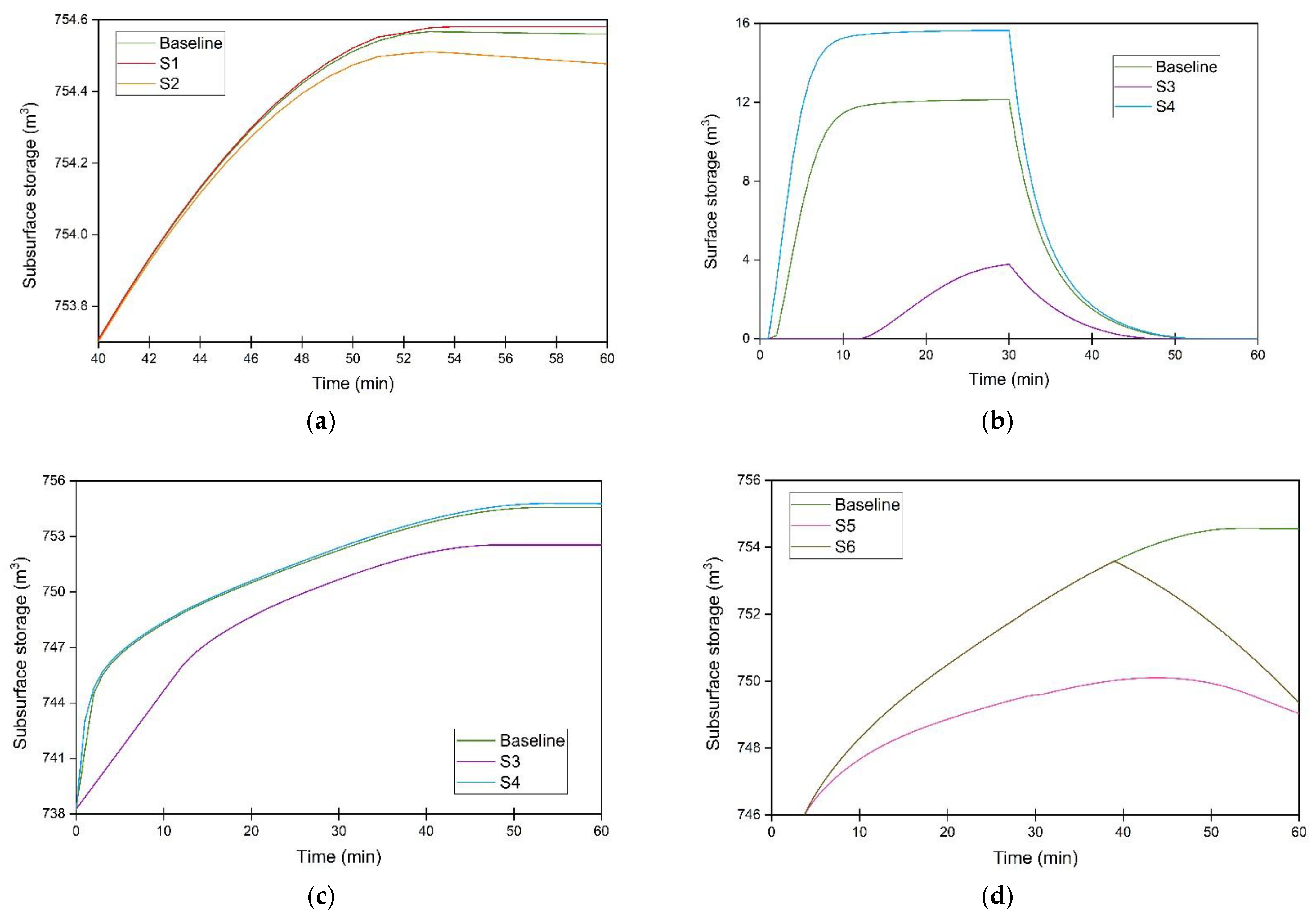
- More complex conceptualization is configured in the DYK domain, with primary model geometry, and several inputs are from in-situ measurements. Meanwhile, the simulations are driven by remote sensing and reanalysis products. Seven scenarios are utilized to investigate hydrological responses influenced by natural processes and groundwater exploitations. Surface runoff and subsurface storage volume show different sensitivities to perturbations such as precipitation, evaporation and groundwater exploitation. Moreover, groundwater exploitation is proved to be more influential than natural precipitation and evaporation anomalies using a correlation coefficients heat map.
Author Contributions
Funding
Data Availability Statement
Acknowledgments
Conflicts of Interest
References
- MacDonald, A.M.; Bonsor, H.C.; Ahmed, K.M.; Burgess, W.G.; Basharat, M.; Calow, R.C.; Dixit, A.; Foster, S.S.D.; Gopal, K.; Lapworth, D.J.; et al. Groundwater quality and depletion in the Indo-Gangetic Basin mapped from in situ observations. Nat. Geosci. 2016, 9, 762–766. [Google Scholar] [CrossRef] [Green Version]
- Abbott, B.W.; Bishop, K.; Zarnetske, J.P.; Minaudo, C.; Chapin, F.S.; Krause, S.; Hannah, D.M.; Conner, L.; Ellison, D.; Godsey, S.E.; et al. Human domination of the global water cycle absent from depictions and perceptions. Nat. Geosci. 2019, 12, 533–540. [Google Scholar] [CrossRef] [Green Version]
- Cuthbert, M.O.; Gleeson, T.; Moosdorf, N.; Befus, K.M.; Schneider, A.; Hartmann, J.; Lehner, B. Global patterns and dynamics of climate–groundwater interactions. Nat. Clim. Chang. 2019, 9, 137–141. [Google Scholar] [CrossRef]
- Gorelick, S.M.; Zheng, C. Global change and the groundwater management challenge. Water Resour. Res. 2015, 51, 3031–3051. [Google Scholar] [CrossRef]
- Liu, M.; Jiang, Y.; Xu, X.; Huang, Q.; Huo, Z.; Huang, G. Long-term groundwater dynamics affected by intense agricultural activities in oasis areas of arid inland river basins, Northwest China. Agric. Water Manag. 2018, 203, 37–52. [Google Scholar] [CrossRef]
- Kollet, S.; Sulis, M.; Maxwell, R.M.; Paniconi, C.; Putti, M.; Bertoldi, G.; Coon, E.T.; Cordano, E.; Endrizzi, S.; Kikinzon, E.; et al. The integrated hydrologic model intercomparison project, IH-MIP2: A second set of benchmark results to diagnose integrated hydrology and feedbacks. Water Resour. Res. 2017, 53, 867–890. [Google Scholar] [CrossRef] [Green Version]
- Li, X.; Cheng, G.; Ge, Y.; Li, H.; Han, F.; Hu, X.; Tian, W.; Tian, Y.; Pan, X.; Nian, Y.; et al. Hydrological Cycle in the Heihe River Basin and Its Implication for Water Resource Management in Endorheic Basins. J. Geophys. Res. Atmos. 2018, 123, 890–914. [Google Scholar] [CrossRef]
- Zhang, X.; Ding, N.; Han, S.; Tang, Q. Irrigation-Induced Potential Evapotranspiration Decrease in the Heihe River Basin, Northwest China, as Simulated by the WRF Model. J. Geophys. Res. Atmos. 2020, 125, e2019JD031058. [Google Scholar] [CrossRef]
- Xu, X.; Jiang, Y.; Liu, M.; Huang, Q.; Huang, G. Modeling and assessing agro-hydrological processes and irrigation water saving in the middle Heihe River basin. Agric. Water Manag. 2019, 211, 152–164. [Google Scholar] [CrossRef]
- Rozemeijer, J.C.; van der Velde, Y.; McLaren, R.G.; van Geer, F.C.; Broers, H.P.; Bierkens, M.F.P. Integrated modeling of groundwater-surface water interactions in a tile-drained agricultural field: The importance of directly measured flow route contributions. Water Resour. Res. 2010, 46, W11537. [Google Scholar] [CrossRef]
- Fry, T.; Maxwell, R. Using a Distributed Hydrologic Model to Improve the Green Infrastructure Parameterization Used in a Lumped Model. Water 2018, 10, 1756. [Google Scholar] [CrossRef] [Green Version]
- Maxwell, R.M.; Putti, M.; Meyerhoff, S.; Delfs, J.; Ferguson, I.M.; Ivanov, V.; Kim, J.; Kolditz, O.; Kollet, S.J.; Kumar, M.; et al. Surface-subsurface model intercomparison: A first set of benchmark results to diagnose integrated hydrology and feedbacks. Water Resour. Res. 2014, 50, 1531–1549. [Google Scholar] [CrossRef] [Green Version]
- Kumar, M.; Duffy, C.J.; Salvage, K.M. A Second-Order Accurate, Finite Volume-Based, Integrated Hydrologic Modeling (FIHM) Framework for Simulation of Surface and Subsurface Flow. Vadose Zone J. 2009, 8, 873. [Google Scholar] [CrossRef] [Green Version]
- Gentine, P.; Green, J.K.; Guérin, M.; Humphrey, V.; Seneviratne, S.I.; Zhang, Y.; Zhou, S. Coupling between the terrestrial carbon and water cycles-a review. Environ. Res. Lett. 2019, 14, 83003. [Google Scholar] [CrossRef]
- Blöschl, G.; Bierkens, M.F.P.; Chambel, A.; Cudennec, C.; Destouni, G.; Fiori, A.; Kirchner, J.W.; McDonnell, J.J.; Savenije, H.H.G.; Sivapalan, M.; et al. Twenty-three unsolved problems in hydrology (UPH)–a community perspective. Hydrol. Sci. J. 2019, 64, 1141–1158. [Google Scholar] [CrossRef] [Green Version]
- Maina, F.Z.; Siirila-Woodburn, E.R.; Vahmani, P. Sensitivity of meteorological-forcing resolution on hydrologic variables. Hydrol. Earth Syst. Sci. 2020, 24, 3451–3474. [Google Scholar] [CrossRef]
- Foster, L.M.; Williams, K.H.; Maxwell, R.M. Resolution matters when modeling climate change in headwaters of the Colorado River. Environ. Res. Lett. 2020, 15, 104031. [Google Scholar] [CrossRef]
- Fan, Y.; Clark, M.; Lawrence, D.M.; Swenson, S.; Band, L.E.; Brantley, S.L.; Brooks, P.D.; Dietrich, W.E.; Flores, A.; Grant, G.; et al. Hillslope Hydrology in Global Change Research and Earth System Modeling. Water Resour. Res. 2019, 55, 1737–1772. [Google Scholar] [CrossRef] [Green Version]
- Fleckenstein, J.H.; Krause, S.; Hannah, D.M.; Boano, F. Groundwater-surface water interactions: New methods and models to improve understanding of processes and dynamics. Adv. Water Resour. 2010, 33, 1291–1295. [Google Scholar] [CrossRef]
- Simpson, S.C.; Meixner, T. Modeling effects of floods on streambed hydraulic conductivity and groundwater-surface water interactions. Water Resour. Res. 2012, 48, W02515. [Google Scholar] [CrossRef]
- Sulis, M.; Meyerhoff, S.B.; Paniconi, C.; Maxwell, R.M.; Putti, M.; Kollet, S.J. A comparison of two physics-based numerical models for simulating surface water–groundwater interactions. Adv. Water Resour. 2010, 33, 456–467. [Google Scholar] [CrossRef]
- Taylor, K.E.; Stouffer, R.J.; Meehl, G.A. An Overview of CMIP5 and the Experiment Design. Bull. Am. Meteorol. Soc. 2012, 93, 485–498. [Google Scholar] [CrossRef] [Green Version]
- Smith, M.B.; Gupta, H.V. The Distributed Model Intercomparison Project (DMIP)-Phase 2 experiments in the Oklahoma Region, USA. J. Hydrol. 2012, 418–419, 1–2. [Google Scholar] [CrossRef]
- Smith, M.B.; Koren, V.; Reed, S.; Zhang, Z.; Zhang, Y.; Moreda, F.; Cui, Z.; Mizukami, N.; Anderson, E.A.; Cosgrove, B.A. The distributed model intercomparison project-Phase 2: Motivation and design of the Oklahoma experiments. J. Hydrol. 2012, 418, 3–16. [Google Scholar] [CrossRef] [Green Version]
- Kollet, S.J.; Maxwell, R.M. Integrated surface-groundwater flow modeling: A free-surface overland flow boundary condition in a parallel groundwater flow model. Adv. Water Resour. 2006, 29, 945–958. [Google Scholar] [CrossRef] [Green Version]
- Kazezyılmaz-Alhan, C.M.; Medina, M.A.; Rao, P. On numerical modeling of overland flow. Appl. Math. Comput. 2005, 166, 724–740. [Google Scholar] [CrossRef]
- Kazezyılmaz-Alhan, C.M. An improved solution for diffusion waves to overland flow. Appl. Math. Model. 2011, 36, 4165–4172. [Google Scholar] [CrossRef]
- Abdul, A.S.; Gillham, R.W. Laboratory Studies of the Effects of the Capillary Fringe on Streamflow Generation. Water Resour. Res. 1984, 20, 691–698. [Google Scholar] [CrossRef]
- Weill, S.; Mouche, E.; Patin, J. A generalized Richards equation for surface/subsurface flow modelling. J. Hydrol. 2009, 366, 9–20. [Google Scholar] [CrossRef]
- Kuffour, B.N.O.; Engdahl, N.B.; Woodward, C.S.; Condon, L.E.; Kollet, S.; Maxwell, R.M. Simulating coupled surface-subsurface flows with ParFlow v3.5.0: Capabilities, applications, and ongoing development of an open-source, massively parallel, integrated hydrologic model. Geosci. Model Dev. 2020, 13, 1373–1397. [Google Scholar] [CrossRef] [Green Version]
- Maxwell, R.M.; Kollet, S.J. Quantifying the effects of three-dimensional subsurface heterogeneity on Hortonian runoff processes using a coupled numerical, stochastic approach. Adv. Water Resour. 2008, 31, 807–817. [Google Scholar] [CrossRef]
- Engdahl, N.B.; Maxwell, R.M. Quantifying changes in age distributions and the hydrologic balance of a high-mountain watershed from climate induced variations in recharge. J. Hydrol. 2015, 522, 152–162. [Google Scholar] [CrossRef]
- Burstedde, C.; Fonseca, J.A.; Kollet, S. Enhancing speed and scalability of the ParFlow simulation code. Comput. Geosci. 2018, 22, 347–361. [Google Scholar] [CrossRef] [Green Version]
- Lu, Z.; Chai, L.; Liu, S.; Cui, H.; Zhang, Y.; Jiang, L.; Jin, R.; Xu, Z. Estimating Time Series Soil Moisture by Applying Recurrent Nonlinear Autoregressive Neural Networks to Passive Microwave Data over the Heihe River Basin, China. Remote Sens. 2017, 9, 574. [Google Scholar] [CrossRef] [Green Version]
- Liu, S.; Li, X.; Xu, Z.; Che, T.; Xiao, Q.; Ma, M.; Liu, Q.; Jin, R.; Guo, J.; Wang, L.; et al. The Heihe Integrated Observatory Network: A Basin-Scale Land Surface Processes Observatory in China. Vadose Zone J. 2018, 17, 180072. [Google Scholar] [CrossRef]
- Li, X.; Cheng, G.; Liu, S.; Xiao, Q.; Ma, M.; Jin, R.; Che, T.; Liu, Q.; Wang, W.; Qi, Y.; et al. Heihe Watershed Allied Telemetry Experimental Research (HiWATER): Scientific Objectives and Experimental Design. Bull. Am. Meteorol. Soc. 2013, 94, 1145–1160. [Google Scholar] [CrossRef]
- Yao, Y.; Zheng, C.; Liu, J.; Cao, G.; Xiao, H.; Li, H.; Li, W. Conceptual and numerical models for groundwater flow in an arid inland river basin. Hydrol. Process. 2015, 29, 1480–1492. [Google Scholar] [CrossRef]
- Wu, B.; Zheng, Y.; Tian, Y.; Wu, X.; Yao, Y.; Han, F.; Liu, J.; Zheng, C. Systematic assessment of the uncertainty in integrated surface water-groundwater modeling based on the probabilistic collocation method. Water Resour. Res. 2014, 50, 5848–5865. [Google Scholar] [CrossRef]
- Wu, B.; Zheng, Y.; Wu, X.; Tian, Y.; Han, F.; Liu, J.; Zheng, C. Optimizing water resources management in large river basins with integrated surface water-groundwater modeling: A surrogate-based approach. Water Resour. Res. 2015, 51, 2153–2173. [Google Scholar] [CrossRef]
- Tian, Y.; Zheng, Y.; Wu, B.; Wu, X.; Liu, J.; Zheng, C. Modeling surface water-groundwater interaction in arid and semi-arid regions with intensive agriculture. Environ. Model. Softw. 2015, 63, 170–184. [Google Scholar] [CrossRef]
- Liu, S.; Xu, Z.; Song, L.; Zhao, Q.; Ge, Y.; Xu, T.; Ma, Y.; Zhu, Z.; Jia, Z.; Zhang, F. Upscaling evapotranspiration measurements from multi-site to the satellite pixel scale over heterogeneous land surfaces. Agric. For. Meteorol. 2016, 230, 97–113. [Google Scholar] [CrossRef]
- Jones, J.E.; Woodward, C.S. Newton-Krylov-multigrid solvers for large-scale, highly heterogeneous, variably saturated flow problems. Adv. Water Resour. 2001, 24, 763–774. [Google Scholar] [CrossRef] [Green Version]
- Ashby, S.F.; Falgout, R.D. A parallel multigrid preconditioned conjugate gradient algorithm for groundwater flow simulations. Nucl. Sci. Eng. 1996, 124, 145–159. [Google Scholar] [CrossRef]
- Osei-Kuffuor, D.; Maxwell, R.M.; Woodward, C.S. Improved numerical solvers for implicit coupling of subsurface and overland flow. Adv. Water Resour. 2014, 74, 185–195. [Google Scholar] [CrossRef]
- Maxwell, R.M. A terrain-following grid transform and preconditioner for parallel, large-scale, integrated hydrologic modeling. Adv. Water Resour. 2013, 53, 109–117. [Google Scholar] [CrossRef]
- Poeter, E.; Fan, Y.; Cherry, J.; Wood, W.; Mackay, D. Groundwater in Our Water Cycle-Getting to Know Earth’s Most Important Fresh Water Source; The Groundwater Project: Guelph, ON, Canada, 2020. [Google Scholar]
- Di Giammarco, P.; Todini, E.; Lamberti, P. A conservative finite elements approach to overland flow: The control volume finite element formulation. J. Hydrol. 1996, 175, 267–291. [Google Scholar] [CrossRef]
- Panday, S.; Huyakorn, P.S. A fully coupled physically-based spatially-distributed model for evaluating surface/subsurface flow. Adv. Water Resour. 2004, 27, 361–382. [Google Scholar] [CrossRef]
- Akhavan, M.; Imhoff, P.T.; Finsterle, S.; Andres, A.S. Application of a Coupled Overland Flow-Vadose Zone Model to Rapid Infiltration Basin Systems. Vadose Zone J. 2012, 11, vzj2011.0140. [Google Scholar] [CrossRef]
- Nijssen, B.; Bowling, L.C.; Lettenmaier, D.P.; Clark, D.B.; El Maayar, M.; Essery, R.; Goers, S.; Gusev, Y.M.; Habets, F.; van den Hurk, B.; et al. Simulation of high latitude hydrological processes in the Torne–Kalix basin: PILPS Phase 2(e) 2: Comparison of model results with observations. Glob. Planet. Chang. 2003, 38, 31–53. [Google Scholar] [CrossRef] [Green Version]
- Kollet, S.J.; Maxwell, R.M.; Woodward, C.S.; Smith, S.; Vanderborght, J.; Vereecken, H.; Simmer, C. Proof of concept of regional scale hydrologic simulations at hydrologic resolution utilizing massively parallel computer resources. Water Resour. Res. 2010, 46, W04201. [Google Scholar] [CrossRef]
- Hammond, G.E.; Lichtner, P.C.; Mills, R.T. Evaluating the performance of parallel subsurface simulators: An illustrative example with PFLOTRAN. Water Resour. Res. 2014, 50, 208–228. [Google Scholar] [CrossRef] [Green Version]
- Gueymard, C.A. A review of validation methodologies and statistical performance indicators for modeled solar radiation data: Towards a better bankability of solar projects. Renew. Sustain. Energy Rev. 2014, 39, 1024–1034. [Google Scholar] [CrossRef]
- Tian, D.; Liu, D. A new integrated surface and subsurface flows model and its verification. Appl. Math. Model. 2011, 35, 3574–3586. [Google Scholar] [CrossRef]
- Sklash, M.G.; Farvolden, R.N. The role of groundwater in storm runoff. J. Hydrol. 1979, 43, 45–65. [Google Scholar] [CrossRef]
- Song, X.; Brus, D.J.; Liu, F.; Li, D.; Zhao, Y.; Yang, J.; Zhang, G. Mapping soil organic carbon content by geographically weighted regression: A case study in the Heihe River Basin, China. Geoderma. 2016, 261, 11–22. [Google Scholar] [CrossRef]
- Yang, R.; Zhang, G.; Liu, F.; Lu, Y.; Yang, F.; Yang, F.; Yang, M.; Zhao, Y.; Li, D. Comparison of boosted regression tree and random forest models for mapping topsoil organic carbon concentration in an alpine ecosystem. Ecol. Indic. 2016, 60, 870–878. [Google Scholar] [CrossRef]
- Gleeson, T.; Moosdorf, N.; Hartmann, J.; van Beek, L.P.H. A glimpse beneath earth’s surface: GLobal HYdrogeology MaPS (GLHYMPS) of permeability and porosity. Geophys. Res. Lett. 2014, 41, 3891–3898. [Google Scholar] [CrossRef] [Green Version]
- Gao, Y.; Cheng, G.; Liu, W.; Cui, W.; Liu, Y.; Li, H.; Peng, H.; Wang, S. Modification of the Soil Characteristic Parameters in Heihe River Basin and Effects on Simulated Atmospheric Elements. Plateau Meteorol. 2007, 5, 958–966. [Google Scholar]
- Xiong, Z.; Yan, X. Building a high-resolution regional climate model for the Heihe River Basin and simulating precipitation over this region. Chin. Sci. Bull. 2014, 59, 605–614. [Google Scholar] [CrossRef]
- Hartmann, J.; Moosdorf, N. The new global lithological map database GLiM: A representation of rock properties at the Earth surface. Geochem. Geophys. Geosyst. 2012, 13, Q12004. [Google Scholar] [CrossRef]
- Shangguan, W.; Dai, Y.; Duan, Q.; Liu, B.; Yuan, H. A global soil data set for earth system modeling. J. Adv. Model. Earth Syst. 2014, 6, 249–263. [Google Scholar] [CrossRef]
- Wang, Z.; Shi, W. Robust variogram estimation combined with isometric log-ratio transformation for improved accuracy of soil particle-size fraction mapping. Geoderma 2018, 324, 56–66. [Google Scholar] [CrossRef]
- Lu, Z.; Sun, J.; He, Y.; Li, Z.; Peng, S.; Yang, X. Impacts of Subsurface Aquifer Heterogeneity on Surface Heat Fluxes and Temperature: A Case Study in the Irrigation Area in the Middle reaches of the Heihe River Basin. Geogr. Geo-Inf. Sci. 2021, 37, 7–15. [Google Scholar]
- Cui, H. Study on Water Cycle Mechanism and Synergetic Evolution between Water Cycle and Oasis in Heihe River Basin; Northwest University: Xi’an, China, 2016; Volume [D]. [Google Scholar]
- Condon, L.E.; Maxwell, R.M. Groundwater-fed irrigation impacts spatially distributed temporal scaling behavior of the natural system: A spatio-temporal framework for understanding water management impacts. Environ. Res. Lett. 2014, 9, 34009. [Google Scholar] [CrossRef]
- Zhang, X.; Xiong, Z.; Tang, Q. Modeled effects of irrigation on surface climate in the Heihe River Basin, Northwest China. J. Geophys. Res. Atmos. 2017, 122, 7881–7895. [Google Scholar] [CrossRef]
- Martens, B.; Miralles, D.G.; Lievens, H.; van der Schalie, R.; de Jeu, R.A.M.; Fernández-Prieto, D.; Beck, H.E.; Dorigo, W.A.; Verhoest, N.E.C. GLEAM v3: Satellite-based land evaporation and root-zone soil moisture. Geosci. Model Dev. 2017, 10, 1903–1925. [Google Scholar] [CrossRef] [Green Version]
- Zeng, Y.; Xie, Z.; Yu, Y.; Liu, S.; Wang, L.; Zou, J.; Qin, P.; Jia, B. Effects of anthropogenic water regulation and groundwater lateral flow on land processes. J. Adv. Model. Earth Syst. 2016, 8, 1106–1131. [Google Scholar] [CrossRef]
- Hu, G.; Jia, L. Monitoring of Evapotranspiration in a Semi-Arid Inland River Basin by Combining Microwave and Optical Remote Sensing Observations. Remote Sens. 2015, 7, 3056–3087. [Google Scholar] [CrossRef] [Green Version]
- Song, L.; Liu, S.; Kustas, W.P.; Nieto, H.; Sun, L.; Xu, Z.; Skaggs, T.H.; Yang, Y.; Ma, M.; Xu, T.; et al. Monitoring and validating spatially and temporally continuous daily evaporation and transpiration at river basin scale. Remote Sens. Environ. 2018, 219, 72–88. [Google Scholar] [CrossRef]
- Zhang, M.; Wang, S.; Fu, B.; Gao, G.; Shen, Q. Ecological effects and potential risks of the water diversion project in the Heihe River Basin. Sci. Total Environ. 2018, 619, 794–803. [Google Scholar] [CrossRef]
- Cheng, G.; Li, X.; Zhao, W.; Xu, Z.; Feng, Q.; Xiao, S.; Xiao, H. Integrated study of the water–ecosystem–economy in the Heihe River Basin. Natl. Sci. Rev. 2014, 1, 413–428. [Google Scholar] [CrossRef] [Green Version]
- Zhao, C.; Wang, P.; Zhang, G. A comparison of integrated river basin management strategies: A global perspective. Phys. Chem. Earth Parts A/B/C 2015, 89, 10–17. [Google Scholar] [CrossRef]
- Wang, G.; Chen, J.; Zhou, Q.; Chu, X.; Zhou, X. Modelling analysis of water-use efficiency of maize in Heihe River Basin. Phys. Chem. Earth Parts A/B/C 2016, 96, 50–54. [Google Scholar] [CrossRef]
- Condon, L.E.; Maxwell, R.M. Feedbacks between managed irrigation and water availability: Diagnosing temporal and spatial patterns using an integrated hydrologic model. Water Resour. Res. 2014, 50, 2600–2616. [Google Scholar] [CrossRef]


| Numerical Methods | ParFlow |
|---|---|
| Subsurface flow governing equation | Richards |
| Surface flow governing equation | Kinematic wave |
| Subsurface numerical approach | Finite difference |
| Surface numerical approach | Upward finite volume |
| Saturated-unsaturated coupling | Entire continuum |
| Subsurface-surface coupling | Free-surface boundary condition |
| Coupling strategy | Implicit |
| Discretization | Rectangular |
| Grid capacity | Structured and semi-unstructured |
| Category | Case | Reference | Auxiliary |
|---|---|---|---|
| Overland flow | Case 1: 1D parking lot | Analytical solution [26,27] | PFLOTRAN, Cast3M |
| Case 2: 2D tilted V-catchment | Di Giammarco et al. [47,48] | PFLOTRAN, WATLAC | |
| Integrated groundwater-surface water flow | Case 3: 2D sandbox | Laboratory experiment data [49] | InHM, ISWGM |
| Unit | 1D Parking Lot | 2D V-Catchment | 2D Sandbox | ||
|---|---|---|---|---|---|
| Model geometry | Horizontal size | m | 180 | 1620 × 1000 | 1.4 × 0.08 |
| Horizontal resolution | m | 1.8/18 | 20 | 0.01 | |
| Vertical resolution | m | 0.5 | 0.5 | 0.01 | |
| Time configuration | Simulation period | s | 3600 | 10,800 | 1500 |
| Rain duration | s | 1800 | 5400 | 1200 | |
| Recession duration | s | 1800 | 5400 | 300 | |
| Time step size | s | 60 | 60 | 10 | |
| Boundary conditions | Lateral and bottom | No flow | |||
| Surface toe | Overland flow | ||||
| Overland flow | Zero depth gradient outlet | ||||
| Initial condition | Water table | m | Subsurface saturated | Subsurface saturated | 0.74 above bottom |
| Surface coefficients | Rain rate | m/s | 1.4 × 10⁻⁵ | 3 × 10⁻⁶ | |
| X direction slope | - | 0.0016 | 0 (channel) 0.05 (slope) | ||
| Y direction slope | - | 0 | 0.02 | ||
| Manning’s roughness | 4.2 × 10⁻⁴ | 2.5 × 10⁻³ (channel) 2.5 × 10⁻⁴ (slope) | |||
| Subsurface hydraulic coefficients | Saturated hydraulic conductivity | m/s | 3.5 × 10⁻⁵ | ||
| Specific storage | m−1 | 10−4 | |||
| Porosity | - | 0.34 | |||
| Van Genuchten Parameters | |||||
| Pore-size radius (α) | m−1 | 2.4 | |||
| Pore-size distribution (n) | - | 5.0 | |||
| Res. vol. water content | - | 0.2 | |||
| Sat. vol. water content | - | 1.0 | |||
| Unit | Value | ||
|---|---|---|---|
| Model geometry | Domain size | m | 850 × 1 × 4 |
| Horizontal resolution | m | 10 | |
| Vertical resolution | m | 0.01 | |
| Subsurface hydraulic coefficients | Saturated hydraulic conductivity | m/s | 1.0 × 10⁻⁵ |
| Porosity | 0.22 | ||
| Van Genuchten Parameters | |||
| Pore-size radius (α) | m−1 | 5.0 | |
| Pore-size distribution (n) | 1.6 | ||
| Res. vol. water content | 0.015 | ||
| Sat. vol. water content | 0.29 | ||
| Surface coefficients | Evaporation rate | m/s | 4.17 × 10⁻⁵ |
| Rain rate | m/s | Observed | |
| Slope | −0.0024 | ||
| Manning’s roughness | 2.5 × 10⁻³ | ||
| Initial condition | Groundwater table depth | m | Steady-state |
| Boundary conditions | Bottom | No flow | |
| Front and back | No flow | ||
| Left and right | Time-series observed | ||
| Unit | Shallow Layer | Deep Layer | ||
|---|---|---|---|---|
| Model geometry | Layer depth | m | 2 | 5 |
| Subsurface hydraulic coefficients | Saturated hydraulic conductivity | m/s | 3 × 10⁻⁶ | 8.5 × 10⁻⁶ |
| Porosity | 0.4589 | 0.4102 | ||
| Van Genuchten Parameters | ||||
| Pore-size radius (α) | m−1 | 1.03 | 2.3 | |
| Pore-size distribution (n) | 1.174 | 1.254 | ||
| Res. vol. water content | 0.02 | 0.04 | ||
| Sat. vol. water content | 0.437 | 0.349 | ||
| Surface coefficients | Slope | 0.25 | ||
| Manning’s roughness | 2.5 × 10⁻³ | |||
| Initial condition | Groundwater table depth | m | 5 | |
| Boundary conditions | Lateral and bottom | No flow | ||
| Surface toe | Overland flow | |||
| Overland flow | Zero depth gradient outlet | |||
| Scenarios | Rainfall Rate | Evaporation Rate | Pumping Rate | Pumping Period |
|---|---|---|---|---|
| Baseline | 6.67 × 10⁻⁵ m/s | 1.8 mm/day | 0 | - |
| 1 | 6.67 × 10⁻⁵ m/s | 0 | 0 | - |
| 2 | 6.67 × 10⁻⁵ m/s | 9 mm/day | 0 | - |
| 3 | 2.5 × 10⁻⁵ m/s | 1.8 mm/day | 0 | - |
| 4 | 1.0 × 10⁻⁴ m/s | 1.8 mm/day | 0 | - |
| 5 | 6.67 × 10⁻⁵ m/s | 1.8 mm/day | 3.33 × 10⁻⁴ m3/s | 0–3600 s |
| 6 | 6.67 × 10⁻⁵ m/s | 1.8 mm/day | 1.0 × 10⁻³ m3/s | 2400–3600 s |
Disclaimer/Publisher’s Note: The statements, opinions and data contained in all publications are solely those of the individual author(s) and contributor(s) and not of MDPI and/or the editor(s). MDPI and/or the editor(s) disclaim responsibility for any injury to people or property resulting from any ideas, methods, instructions or products referred to in the content. |
© 2023 by the authors. Licensee MDPI, Basel, Switzerland. This article is an open access article distributed under the terms and conditions of the Creative Commons Attribution (CC BY) license (https://creativecommons.org/licenses/by/4.0/).
Share and Cite
Lu, Z.; He, Y.; Peng, S. Assessing Integrated Hydrologic Model: From Benchmarking to Case Study in a Typical Arid and Semi-Arid Basin. Land 2023, 12, 697. https://doi.org/10.3390/land12030697
Lu Z, He Y, Peng S. Assessing Integrated Hydrologic Model: From Benchmarking to Case Study in a Typical Arid and Semi-Arid Basin. Land. 2023; 12(3):697. https://doi.org/10.3390/land12030697
Chicago/Turabian StyleLu, Zheng, Yuan He, and Shuyan Peng. 2023. "Assessing Integrated Hydrologic Model: From Benchmarking to Case Study in a Typical Arid and Semi-Arid Basin" Land 12, no. 3: 697. https://doi.org/10.3390/land12030697