Article

Economic Growth Does Not Mitigate Its Decoupling Relationship with Urban Greenness in China

1
Institute of Land and Urban-Rural Development, Zhejiang University of Finance and Economics, Hangzhou 310018, China
2
Dongfang College, Zhejiang University of Finance and Economics, Jiaxing 314408, China
*
Author to whom correspondence should be addressed.
Land 2023, 12(3), 614; https://doi.org/10.3390/land12030614
Submission received: 4 February 2023 / Revised: 2 March 2023 / Accepted: 3 March 2023 / Published: 4 March 2023
(This article belongs to the Special Issue Ecosystem Services in Urban Contexts: Balancing City Environment)

Abstract

:
Accompanied by China’s rapid economic growth, significant urban greening has occurred in Chinese cities, in particular in the urban core areas. In contrast, rapid urbanization and economic growth also led to a high probability of vegetation degradation in urban fringe regions. However, these significant spatial differences in urban greenness associated with economic growth in Chinese cities are not well understood. This study explored the spatiotemporal characteristics of the nighttime light (NTL) and annual maximum enhanced vegetation index (EVImax) in urban areas from 2001 to 2020. A strong decoupling status between economic growth and urban greenness on the national scale was found. Overall, 49.15% of urban areas showed a decoupling status. Spatially, this percentage of urban areas with a decoupling status would significantly decrease when the long-term average NTL surpasses 51. Moreover, this significant threshold of decoupling status was found in 189 cities out of 344 (54.65%) in China. This threshold in each city showed significant spatial heterogeneity but can mostly be attributed to the gradient in the long-term average precipitation (Pmean) of each city during the period of 2001–2020. Specifically, a spatial increase in Pmean of 100 mm responded to a decrease in the threshold of 0.4 DN (p < 0.01). In contrast, there was no significant correlation between the threshold and the economic growth status of each city. Our results provide valuable insights for coordinating the development of urban greening and economic growth.

1. Introduction

Urbanization is a complex and multifaceted process involving demographic, economic, and environmental processes. At present, China’s urbanization has become a notable global event, regarded as one of the two key factors deeply influencing urban sustainable development in the 21st century [1,2,3]. Risk from urban environmental pollution and degradation is becoming an explicit threat to human health because of rapid economic growth and urbanization [4,5]. Moreover, much of the literature has also shown that economic development improves urban greening [6,7,8,9]. These complexities of the economy–environment relationship in urban areas are compromising the goal of sustainable urbanization [10,11,12]. However, few studies have examined these complexities of economy–environment dynamics because of the different levels of socioeconomic development and green space.
Economic growth contributes to the goals of achieving sustainable urban development. Hence, obtaining accurate information on the spatial dimensions of economic activities is important for understanding the urban economic status. The statistical data, however, only provide numeric records for specific administrative regions and the accurate spatial distribution of economic status only in urban areas. Fortunately, nighttime light data (NTL) provide a spatial insight into the intensity of artificial light at night on the Earth’s surface and are widely used to monitor various variables, including urbanization, density, and economic growth [13,14]. Many studies have shown that the NTL can provide us with effective proxy measures of spatially explicit dynamics of economic activity in urban areas [14,15,16]. For example, Shi et al. [17] showed that the NTL data can be a powerful tool for modeling socioeconomic indicators. More recently, Chen et al. [18] calculated a global 1 km × 1 km gridded revised real GDP based on calibrated nighttime light data. Therefore, we employed the NTL to monitor economic growth in urban areas in China.
As a major part of sustainable urban development, vegetation plays an important role in providing ecological services in urban areas [7,19,20,21]. Previous studies have shown that two major driving factors affect vegetation dynamics in urban areas [19,22,23]. Firstly, climate factors such as temperature and precipitation provide the necessary conditions for vegetation growth [22,24,25]. Meanwhile, economic growth or human activities also influence essential ecosystem functions, which are also regarded as an important driver of vegetation dynamics in urban areas [26,27,28]. In recent decades, a large amount of resources were invested to improve the urban environment in China [29,30]. As a result, prevalent vegetation greening was observed in urban environments, particularly in the urban core areas [7,22,31,32,33]. For example. Li, Wu, Liang, and Li [22] found that urban areas with greening trends account for about 63% of the Yangtze River Delta. Sun, Chen, Li, and Huang [7] also showed that China accounts for 32% of greening of built-up areas in 841 large cities globally. In contrast, previous studies demonstrated that economic growth and rapid urbanization also induced vegetation degradation in surrounding urban areas [27,28,34,35,36]. This ecosystem degradation resulting from economic growth and urbanization is still an obvious threat to urban sustainable development [11].
To address the insufficiencies mentioned above, the relationships between economic growth and vegetation dynamics showed significant spatial differentiation in the urban core and fringe areas. Moreover, due to the different levels of socioeconomic development, the spatial differentiation within the city is uneven across different cities in China [6,7]. Although the characteristics of urban green spaces were explored in many previous studies, including their abundance, spatial distribution, vegetation dynamics, gross primary production, etc. [31,33,37,38]. The possible spatial thresholds of the different relationships between economic growth and greenness in the urban core and fringe areas have rarely been considered. More importantly, the uneven spatial heterogeneity of this possible threshold across different cities and its responses to economic factors or climate change remain largely unclear. Hence, our work was mainly focused on the following questions to fill this knowledge gap: (1) What are the possible relationships between economic growth and urban greenness? (2) Is there a threshold that can characterize the different relationships between economic growth and greenness in different urban areas? (3) Can economic growth influence this threshold? Understanding the mechanisms of vegetation growth and its relationships with economic growth in urban areas is essential for maintaining ecological service functions and promoting sustainable urban development. Our quantitative study of the underlying relationships between economic growth and urban greenness could be vital to achieving sustainable urban development.

2. Materials and Methods
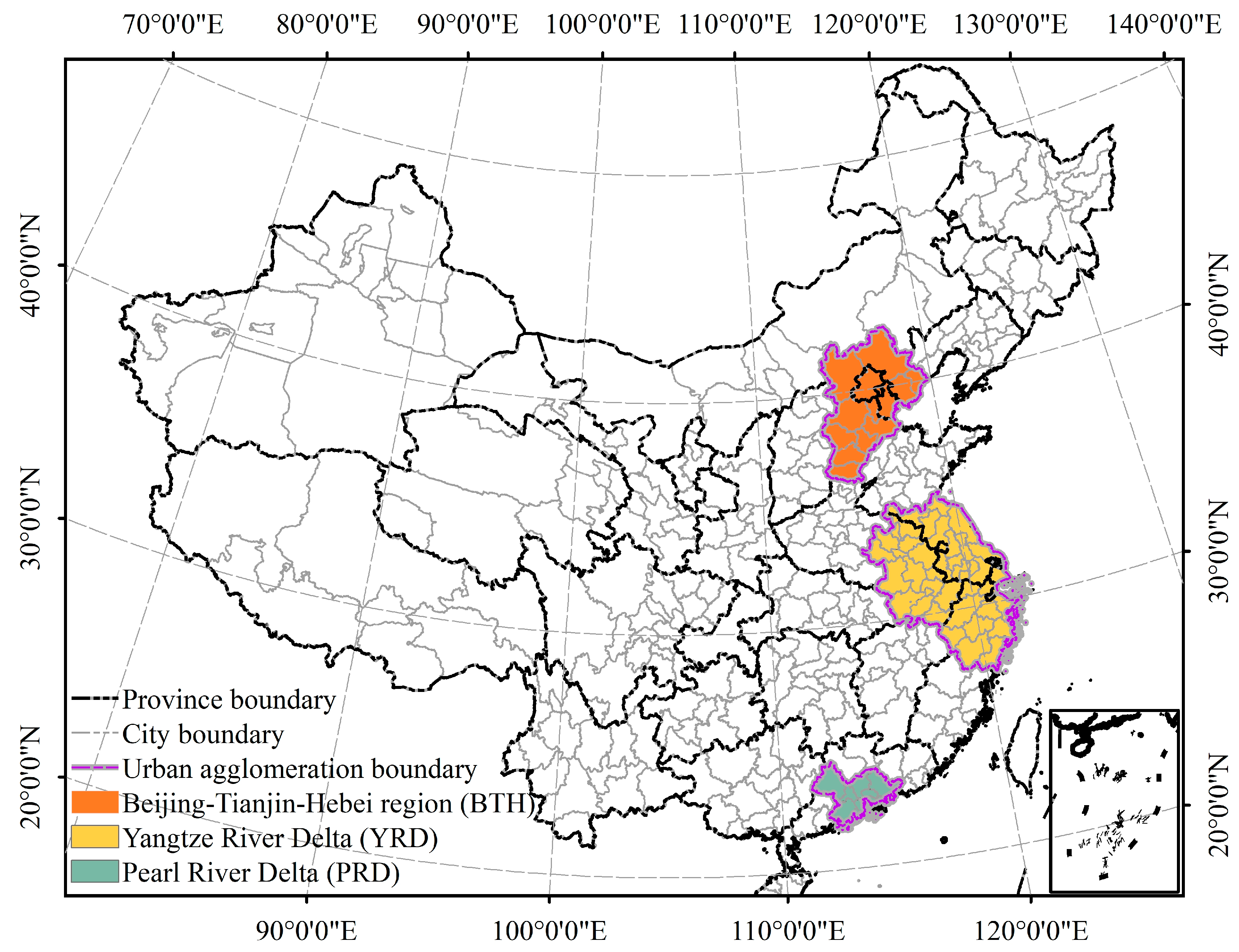
2.1. Study Area

The spatiotemporal variations of economic growth and greenness in urban areas and their possible relationships were analyzed in 344 prefecture-level cities in China (Figure 1). In addition, three typical mega-urban agglomerations were selected for further analysis of the spatiotemporal heterogeneity of economic growth and urban greenness. As the three biggest urban agglomeration areas of China, although rapid economic growth and urbanization have been found in these urban agglomerations, some studies have shown that the vegetation dynamics in these urban agglomerations are different [7,22]. Hence, the different characteristics and relationships between economic growth and urban greenness were analyzed in these three urban agglomerations.

2.2. Urban Areas Extraction

We extracted the urban areas in each city from the International Geosphere-Biosphere Programme (IGBP) classification type dataset at a 500 m spatial resolution, which was provided by the Moderate Resolution Imaging Spectroradiometer (MODIS) land cover type product (MCD12Q1) [39]. To reduce the spurious land cover changes caused by classification uncertainty in each year, this dataset incorporates hidden Markov models and a state-space multitemporal modeling framework. Eventually, pixels with at least 30% impervious surface area were classified as urban and built-up land. Moreover, to avoid the possible decrease in greenness caused by land use changes in expanding urban areas, we only studied the areas in each city that had been converted to urban areas before 2001. The interannual variability of the economic growth and vegetation dynamics during the period 2001–2020 and their relationships were identified in these urban areas.

2.3. The Nighttime Lights of Urban Areas

The nighttime light data (NTL) provided a unique spatial insight into the intensity of artificial lights, and they are widely used to monitor economic growth in urban areas. In this study, a harmonized nighttime light dataset with digital numbers (DN) ranging from 0 to 63 at a 30-arc-second spatial resolution was used as the economic growth indicator [40]. Furthermore, pixels in urban areas with DN values below 10 were excluded due to their uncertainties. To match the spatial resolution of urban area data, these harmonized NTL time series data were resampled to a spatial resolution of 500 m in ArcGIS software. Firstly, the trend of NTL values in each pixel was calculated to analyze its relationship with urban greenness. Furthermore, the mean NTL in each pixel during the period of 2001–2020 was calculated. The mean NTL in each pixel was used as the indicator to predict the thresholds of the decoupling relationship in each city. Finally, the long-term average NTL in all pixels in urban areas (NTLmean) in each city over 2001–2020 was calculated to indicate the economic factor of the city.

2.4. Vegetation Index Data

The enhanced vegetation index (EVI) obtained from MOD13A1 version 6.1 at 500-m spatial resolution and a 16-day temporal resolution from 2002 to 2020 was used in our study [41]. EVI has been found to be one of the best indicators of vegetation status in urban areas because of its greater sensitivity and partial elimination of the effect of canopy background in many studies [7,33,42,43]. To avoid the influence of vegetation phenology, the annual maximum EVI (EVImax) generated from this annual EVI time series was used to indicate urban greenness.

2.5. Climate Data

The gridded temperature and precipitation datasets with 1 km resolution from 2001 to 2020 were obtained from the Science Data Bank [44] and the National Tibetan Plateau Data Center [45], respectively. Similarly, these datasets were resampled to a spatial resolution of 500 m to match the spatial resolution of urban area data in ArcGIS software. The long-term average temperature (Tmean) and precipitation (Pmean) in all urban areas in each city during the period of 2001–2020 were calculated as the climate factors of each city.

2.6. Defining Decoupling Relationship between NTL and EVImax

The conclusion that economic development results in changes in vegetation dynamics are widely accepted. In the context of urban ecological civilization construction in China, urban greening is closely related to economic growth, as cities with high economic growth often prioritize the improvement of the living environment by creating green spaces [6,46,47,48]. However, some cities also experienced a high probability of vegetation degradation because of the rapid economic growth [22,47]. In our study, this relationship between vegetation degradation and economic growth in urban areas was defined as the decoupling relationship. Based on the decoupling index between two indicators [49,50], the different characteristics and relationships between NTL and EVImax in each pixel in urban areas were calculated according to their interannual trends during the period of 2001–2020. The specific classification and logic possibilities are summarized in Table 1.

2.7. The Threshold Detection and Its Responses to Each Factor

A piecewise linear regression method was used to quantitatively detect the potential turning point (TP) of economic growth [51].
y = { β 1 x + β 0 + ε x α β 1 x + β 2 ( x α ) + β 0 + ε x > α
where y is the percentage of urban areas; x is the long-term average NTL value during the period of 2001–2020; α is the estimated TP of the average NTL; β0, β1, and β2 are the regression coefficients; and ε is the residual. The linear trends before and after TP are β1 and (β1 + β2), respectively. This piecewise fitting is obtained optimally when the residual sum of squares is minimized [52,53]. All statistical analyses were performed in R version 4.1.2 [54].
In summary, the threshold of the decoupling relationship between NTL and EVImax was first identified along the urban spatial gradient, with different NTL values in each city. In addition, to understand the spatial heterogeneity of the threshold and its response to each factor, we performed a temporal partial correlation analysis and a linear regression, in which the threshold of each city was set as the dependent variable and the long-term average NTL (NTLmean), temperature (Tmean), and precipitation (Pmean) in all urban pixels in each city were set as independent indicators.

3. Results

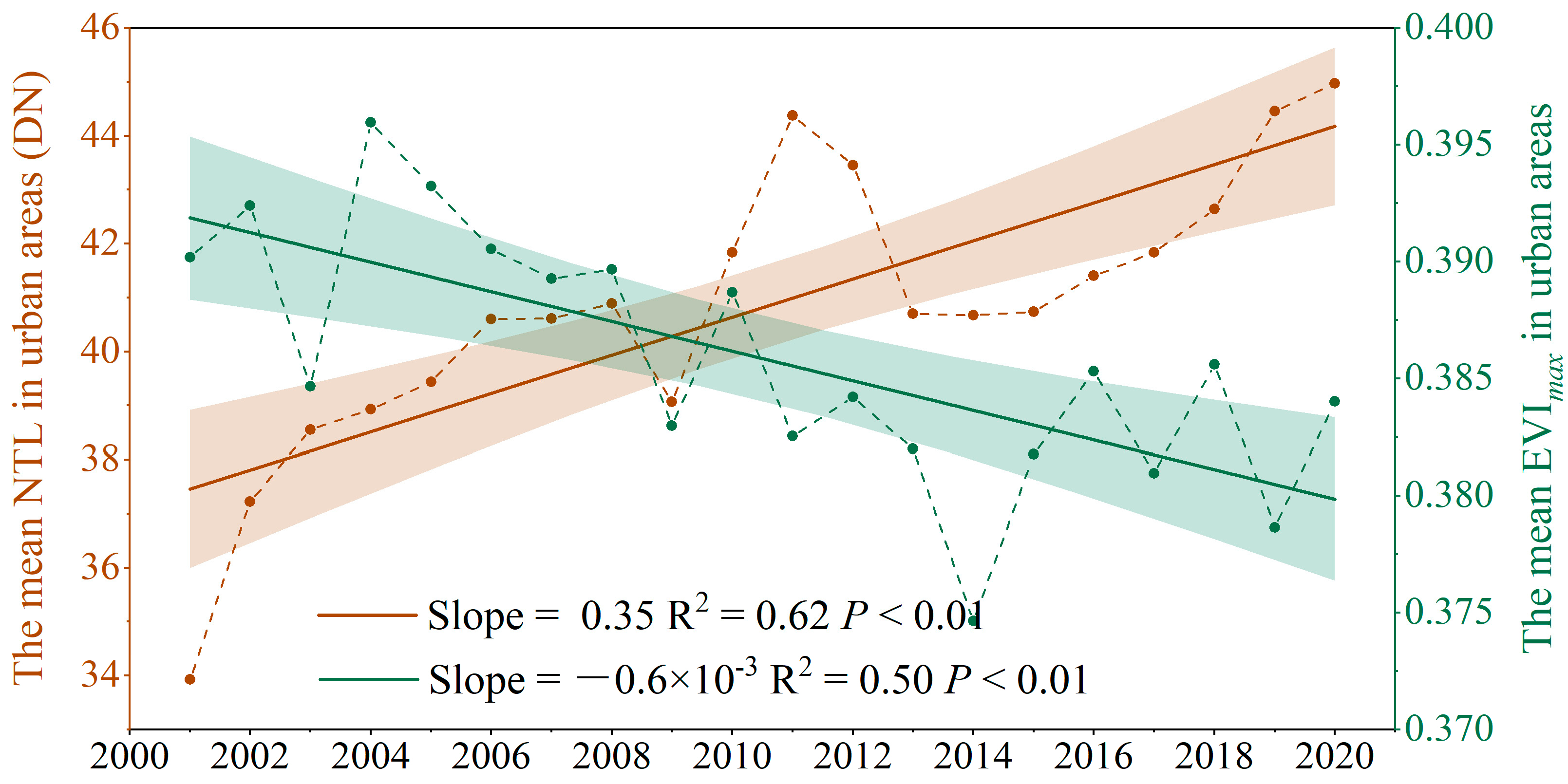
3.1. Decoupling Relationship between NTL and EVImax

A major factor contributing to the improvement of urban vegetation was economic growth. Unfortunately, although the mean NTL in urban areas increased strongly, the mean EVImax showed a decreasing trend. Specifically, the mean NTL in all urban areas in China increased strongly from 2001 to 2020, with an increasing trend of 0.35 DN year−1 (p < 0.01), while the mean EVImax in all urban areas in China showed a significant decreasing trend, with the mean EVImax decreasing by 0.6 × 10⁻³ per year (p < 0.01) (Figure 2). These contrasting interannual variabilities of the mean NTL and the mean EVImax indicated a strong decoupling status between economic growth and urban greenness. Moreover, this decoupling status between economic growth and urban greenness was also found in each city and urban agglomeration (Figure 3).
At the national level, 49.15% of pixels in urban areas showed a decoupling status, and 22.96% of urban areas showed a strong decoupling status. In contrast, 38.60% of pixels in urban areas showed a coupling status, while only 13.99% of pixels showed a strong coupling status. The percentage of urban areas with decoupling status in each city is shown in Figure 3. More than 60% of urban areas have a decoupling status in 107 cities out of 344 (31.10%). Moreover, we found that the decoupling status in urban areas in different mega-urban agglomerations clearly showed spatial heterogeneity and aggregation effects. Specifically, only 15.46% of pixels showed a coupling status, usually located in the core of central urban areas. Meanwhile, 41.28% of pixels showed a decoupling status, mainly located in the surrounding urban areas (Figure 3). This high percentage of urban areas with a decoupling status was also found in the BTH agglomeration. From the spatial pattern of the different relationships between NTL and EVImax in urban areas, we found that many cities are shaped as a “fried egg”. The economic growth and the urban greenness in “yolk-shaped” urban core areas showed coupling status, while more pixels displayed a decoupling status in urban fringe “egg white” areas.

3.2. Thresholds of Decoupling Status

The different relationships between NTL and EVImax in different urban areas implied a possible threshold, which can explain the “fried egg” phenomenon. Hence, we assume that when NTL reaches a certain extent, the percentage of urban areas with decoupling status will begin to rapidly decline. In actuality, we found that the spatial pattern of the decoupling status between NTL and EVImax was strongly affected by the long-term average NTL (Figure 4). Specifically, the percentage of urban areas with a decoupling status (Pattern I, pixels with increasing NTL but decreasing EVImax) was significantly increased by 0.92% DN−1 (p < 0.01) in the interval where the NTL value was less than 51. Afterward, the percentage of urban areas with a decoupling status decreased sharply, with a slope of −3.67% DN−1 (p < 0.01). That is, the percentage of urban areas with a decoupling status increased with the economic growth in the urban areas with a less-developed economic status. Moreover, this significant threshold effect indicated that the decoupling status between economic growth and urban greenness would be gradually relieved and may even be achieved simultaneously under good economic conditions. The lower the threshold, the higher the possibility of a positive synergy between economic growth and urban greenness.
Based on the piecewise linear regression method, the threshold of the decoupling status between NTL and EVImax was detected in each city (Figure 5). The threshold was found in 189 cities out of 344 (54.65%), which were mostly located in the eastern half of the country. Overall, the thresholds of decoupling status in most cities were greater than 40. Spatially, the thresholds in 103 cities out of 189 (54.49%) were greater than 50. In contrast, only 2.11% of cities had a threshold of less than 40. This low threshold was mostly found in the developed cities of China. For example, the threshold of decoupling status between NTL and EVImax in Beijing, Shanghai, and Hangzhou was 27, 41, and 35, respectively.

3.3. Responses of the Threshold to Climate and Economic Factors

Spatially, the threshold of decoupling status in each city was lower in the wetter areas of China (Figure 5). We found that the threshold of decoupling status was negatively correlated with Pmean in each city on the national scale, with a partial correlation coefficient of −0.27 (p < 0.01) (Table 2). In contrast, there was no significant correlation between the threshold of decoupling status and the NTLmean or Tmean in each city (p > 0.10). The sensitivity of the threshold of decoupling status to each factor further showed a stronger impact of Pmean on the threshold of decoupling status than NTLmean and Tmean. The sensitivity of the threshold of decoupling status to Pmean was −0.004 DN mm−1 (p < 0.01) on the national scale. In addition, we also performed partial correlation analyses and calculated the sensitivity of the threshold of decoupling status to each factor in three urban agglomerations. This significant correlation between the threshold of decoupling status and Pmean was also found in YRD, with a partial correlation coefficient of −0.40 (p < 0.01) and a sensitivity of −0.002 DN mm−1 (p < 0.01). Unfortunately, this significant partial correlation coefficient between the threshold of decoupling status and Pmean was not observed in BTH and PRD. The low number of cities with a threshold of decoupling status in these two urban agglomerations may obscure this relevance.
The long-term average precipitation gradient in each city can fully explain the spatial heterogeneities at the threshold of decoupling status (Figure 6). Based on the threshold averaged from each 100-mm bin of Pmean, a 100-mm increase in Pmean responded to a decrease in the threshold of decoupling status of 0.4 DN (p < 0.01). Moreover, the spatial correlation between the threshold of decoupling status and the Pmean in all cities with a threshold of decoupling status was explored (Figure 6, inset). There was also a significant negative spatial correlation between the threshold of decoupling status and Pmean (R = 0.44, p < 0.01).

4. Discussion

4.1. Threshold Effect of Decoupling Status

At the pixel levels, 49.15% of urban areas showed a decoupling status between economic growth and urban greenness, and 22.96% of urban areas showed a strong decoupling status. In contrast, 38.60% of pixels in the urban areas showed a coupling status. Similarly, some studies also found that this greening and browning of vegetation with rapid economic growth coexisted in the different urban areas [7,9,22,55].
Spatially, areas with this coupling status were mainly found in the core of urban areas (Figure 3 inset). This positive synergy between NTL and EVImax matches previous studies that found longer growing seasons and greening changes in the core of the central urban areas compared to their surrounding areas [7,18,22,43,56,57]. China has invested a great deal of resources to improve the urban environment [29,30]. Hence, obvious spatial variation was found regarding the influence of economic factors on urban greening [6,7,22]. In urban core areas with higher economic prosperity, urban vegetation protection and afforestation were given more attention and management by the local government. Any newly constructed park or green space, as well as the growth of street vegetation, can promote vegetation growth [7,33,58]. In contrast, rapid economic and demographic growth was accompanied by high energy demand and environmental pollution, which indirectly contributed to deforestation in the surrounding urban areas [22,59].
In summary, these differing relationships between NTL and EVImax in different urban areas implied the possible threshold effect; that is, only when NTL reaches a certain extent, does the percentage of urban areas with a strong decoupling status begin to rapidly decline. In this case, the decoupling status between economic growth and urban greenness would be gradually relieved and may even be achieved simultaneously under good economic conditions. Under these good economic conditions, the demand for a high-quality living environment and services is stimulated, in particular, a greater quantity and higher quality of urban greenness [11,22,60]. In contrast, before economic conditions reach this threshold, the degradation of the urban ecosystem caused by economic growth will still be a major impediment to sustainable urban development.

4.2. The Drivers of the Threshold of Decoupling Status

Spatially, the threshold of decoupling status in each city was lower in southeastern China (Figure 5). Similarly, Li, Wang, Liu, Li, Zhang, Sun, and Wang [6] showed that the cities showed less socioeconomic development in the northwestern region and had less urban greening. Our results show that the threshold of decoupling status was negatively correlated with long-term average annual accumulated precipitation (Pmean) in each city, with a significant partial correlation coefficient and sensitivity on the national scale (Table 2). In contrast, there was no significant correlation between the threshold of decoupling status and the long-term average NTL (NTLmean) or temperature (Tmean) in each city. That is, economic growth does not reduce the threshold of decoupling status and mitigate its decoupling relationship with urban greenness in China. Although some studies demonstrated that economic growth was a driver of vegetation dynamics by promoting effective green strategies in urban areas [11,61,62,63], these positive synergies between economic growth and urban greenness were only found in the urban core areas [7,32]. In contrast, frequent economic activities caused the great degradation of areas in urban fringe regions [63,64]. Hence, economic growth does not reduce the threshold of decoupling status and mitigate its decoupling relationship with urban greenness in all urban areas. Instead, the Pmean plays a crucial role in reducing the threshold of decoupling status between NTL and EVImax. This important influence of precipitation on vegetation dynamics in urban areas was also found in some studies [22,65]. It has been shown that changes in precipitation have a profound impact on vegetation growth in arid and semi-arid regions [65,66,67,68], because better thermal and hydraulic conditions are likely to enhance the photosynthetic capacity of vegetation by accelerating chemical reactions, which would improve the greenness [68,69]. Drought risks resulting from climate change are intensifying in urban areas [70,71]. Consequently, the higher Pmean in these relatively moist cities would promote vegetation growth in all urban areas and reduce the threshold of decoupling status between NTL and EVImax, thereby mitigating the decoupling relationship between economic growth and urban greenness.

4.3. Uncertainties and Further Studies

Based on the different trends of NTL and EVImax, the spatio-temporal relationship between economic growth and vegetation dynamics was revealed in urban areas in China during the period of 2001–2020. However, some studies showed that the sources of measurement error and uncertainty about the NTL remain largely unclear [72,73,74]. Moreover, some studies also showed their incompatibility with economic development in places where lights react little to changes in economic activity [75,76]. Although an integrated and consistent NTL dataset was used in our study, which harmonized the inter-calibrated NTL observations, there is no way to exclude all noise caused by varying lighting sources [40]. Therefore, the influence of these uncertainties needs to be further mitigated with more models. In addition, the vegetation dynamics were influenced by many other factors, for example, CO2 fertilization [25], water availability [65], and other unstudied factors [22]. Hence, a more comprehensive analysis with more factors should be conducted to analyze the complex and varying limitations on the threshold effect of decoupling status between economic growth and urban greenness. Nevertheless, our present work found a significant threshold effect of the decoupling status between economic growth and urban greenness, found a stronger sensitivity of the threshold of decoupling status to long-term average precipitation, and highlighted that economic growth does not mitigate its decoupling relationship with urban greenness in China, which would provide a useful guideline and valuable insights for coordinating the development of urban greening and economic growth.

5. Conclusions

The nighttime light data (NTL) and annual maximum enhanced vegetation index (EVImax) are widely regarded as effective indicators for monitoring economic growth and greenness in urban areas. Based on the different trends of the NTL and EVImax, the spatio-temporal relationship the economic growth and urban greenness was revealed during the period of 2001–2020. As originally conceived for sustainability, economic growth is an essential and important driver for achieving ecological sustainability. Unfortunately, although the mean NTL in all urban areas in China increased strongly, with an increasing trend of 0.35 DN year−1 (p < 0.01), the mean EVImax in all urban areas showed a decreasing trend, with the mean EVImax decreasing by 0.6 × 10⁻³ per year (p < 0.01). These contrasting interannual variabilities of the mean NTL and the mean EVImax indicated a decoupling status between economic growth and vegetation dynamics in urban areas. Moreover, we found that the decoupling status in urban areas in different mega-urban agglomerations showed obvious spatial heterogeneity and aggregation effect. Specifically, only 15.46% of pixels showed coupling status, which is usually located in the urban core areas. At the same time, 41.28% of pixels showed decoupling status, which was mainly located in the urban fringe areas. To explore this spatial heterogeneity and aggregation effect, a piecewise linear regression method was used to quantitatively detect the potential threshold. At the national level, we found that the percentage of urban areas with decoupling status would significantly decrease, with a slope of −3.67% DN-1 (p < 0.01), when the NTL surpasses 51 DN. Spatially, the long-term average precipitation in each city, rather than economic growth, can fully explain the spatial heterogeneities of the threshold of decoupling. Specifically, a spatial increase in Pmean of 100 mm responded to a decrease in the threshold of 0.4 DN (p < 0.01). In contrast, there was no significant correlation between the threshold and the economic growth status of each city.
Generally, the different relationships between economic growth and vegetation dynamics in urban areas play an important role in monitoring urban sustainable development. However, the relationships between economic growth and vegetation dynamics showed significant spatial differentiation in the urban core and fringe areas. We identified the threshold that explains this spatial differentiation. This threshold in each city can be a valid aid for policymakers in evaluating the level of urban ecological civilization construction in each city. Furthermore, this study constitutes a valuable reference for coordinating the development of urban greening and economic growth.

Author Contributions

Conceptualization, M.C. and Y.L.; methodology, M.C. and C.Z.; software, M.C.; validation, M.C., C.Z., Y.P. and J.Z.; formal analysis, M.C.; data curation, J.W.; writing—original draft preparation, M.C.; writing—review and editing, M.C., Y.L., C.Z., Y.P. and J.Z.; visualization, M.C.; supervision, Y.L.; project administration, M.C. and Y.L.; funding acquisition, Y.L. All authors have read and agreed to the published version of the manuscript.

Funding

This research was funded by the National Natural Science Foundation of China (41901062 and 41901233), and the Natural Science Foundation of Zhejiang Province (LY22D010009, LQ18D010005, and LY20D010007).

Data Availability Statement

The data presented in this study are available on request from the corresponding author.

Acknowledgments

Our deepest gratitude goes to the reviewers and editors for their careful work and detailed suggestions that have helped improve this manuscript.

Conflicts of Interest

The authors declare no conflict of interest.

References

  1. Wu, Y.; Zhang, X.; Shen, L. The impact of urbanization policy on land use change: A scenario analysis. Cities 2011, 28, 147–159. [Google Scholar] [CrossRef]
  2. Normile, D. China Rethinks Cities. Science 2016, 352, 916–918. [Google Scholar] [CrossRef]
  3. Ning, Y.; Liu, S.; Zhao, S.; Liu, M.; Gao, H.; Gong, P. Urban growth rates, trajectories, and multi-dimensional disparities in China. Cities 2022, 126, 103717. [Google Scholar] [CrossRef]
  4. Shi, B.; Jiang, L.; Bao, R.; Zhang, Z.; Kang, Y. The impact of insurance on pollution emissions: Evidence from China’s environmental pollution liability insurance. Econ. Model. 2023, 121, 106229. [Google Scholar] [CrossRef]
  5. Wu, H.; Gai, Z.; Guo, Y.; Li, Y.; Hao, Y.; Lu, Z.-N. Does environmental pollution inhibit urbanization in China? A new perspective through residents’ medical and health costs. Environ. Res. 2020, 182, 109128. [Google Scholar] [CrossRef] [PubMed]
  6. Li, F.; Wang, X.; Liu, H.; Li, X.; Zhang, X.; Sun, Y.; Wang, Y. Does economic development improve urban greening? Evidence from 289 cities in China using spatial regression models. Environ. Monit. Assess. 2018, 190, 541. [Google Scholar] [CrossRef]
  7. Sun, L.; Chen, J.; Li, Q.; Huang, D. Dramatic uneven urbanization of large cities throughout the world in recent decades. Nat. Commun. 2020, 11, 5366. [Google Scholar] [CrossRef]
  8. Wang, H.; Zhao, D.; Zhou, Q.; Ke, Q.; Dong, G. The Coupling Relationship between Green Finance and Ecosystem Service Demand in China Based on an Improved Coupling Coordination Degree Model. Land 2023, 12, 529. [Google Scholar] [CrossRef]
  9. Zhao, S.; Liu, S.; Zhou, D. Prevalent vegetation growth enhancement in urban environment. Proc. Natl. Acad. Sci. USA 2016, 113, 6313–6318. [Google Scholar] [CrossRef] [Green Version]
  10. Fu, B.; Zhang, J.; Wang, S.; Zhao, W. Classification–coordination–collaboration: A systems approach for advancing Sustainable Development Goals. Natl. Sci. Rev. 2020, 7, 838–840. [Google Scholar] [CrossRef] [PubMed] [Green Version]
  11. He, Z.; Xiao, L.; Guo, Q.; Liu, Y.; Mao, Q.; Kareiva, P. Evidence of causality between economic growth and vegetation dynamics and implications for sustainability policy in Chinese cities. J. Clean Prod. 2020, 251, 119550. [Google Scholar] [CrossRef]
  12. Fu, B.; Wang, S.; Zhang, J.; Hou, Z.; Li, J. Unravelling the complexity in achieving the 17 sustainable-development goals. Natl. Sci. Rev. 2019, 6, 386–388. [Google Scholar] [CrossRef] [PubMed] [Green Version]
  13. Zhao, C.; Cao, X.; Chen, X.; Cui, X. A consistent and corrected nighttime light dataset (CCNL 1992–2013) from DMSP-OLS data. Sci. Data 2022, 9, 424. [Google Scholar] [CrossRef] [PubMed]
  14. Levin, N.; Kyba, C.C.M.; Zhang, Q.; Sánchez de Miguel, A.; Román, M.O.; Li, X.; Portnov, B.A.; Molthan, A.L.; Jechow, A.; Miller, S.D.; et al. Remote sensing of night lights: A review and an outlook for the future. Remote Sens. Environ. 2020, 237, 111443. [Google Scholar] [CrossRef]
  15. McCallum, I.; Kyba, C.C.M.; Bayas, J.C.L.; Moltchanova, E.; Cooper, M.; Cuaresma, J.C.; Pachauri, S.; See, L.; Danylo, O.; Moorthy, I.; et al. Estimating global economic well-being with unlit settlements. Nat. Commun. 2022, 13, 2459. [Google Scholar] [CrossRef]
  16. Zhou, Y.; Li, X.; Asrar, G.R.; Smith, S.J.; Imhoff, M. A global record of annual urban dynamics (1992–2013) from nighttime lights. Remote Sens. Environ. 2018, 219, 206–220. [Google Scholar] [CrossRef]
  17. Shi, K.; Yu, B.; Huang, Y.; Hu, Y.; Yin, B.; Chen, Z.; Chen, L.; Wu, J. Evaluating the Ability of NPP-VIIRS Nighttime Light Data to Estimate the Gross Domestic Product and the Electric Power Consumption of China at Multiple Scales: A Comparison with DMSP-OLS Data. Remote Sens. 2014, 6, 1705–1724. [Google Scholar] [CrossRef] [Green Version]
  18. Chen, J.; Gao, M.; Cheng, S.; Hou, W.; Song, M.; Liu, X.; Liu, Y. Global 1 km × 1 km gridded revised real gross domestic product and electricity consumption during 1992–2019 based on calibrated nighttime light data. Sci. Data 2022, 9, 202. [Google Scholar] [CrossRef]
  19. Chen, J.; Yu, Z.; Li, M.; Huang, X. Assessing the Spatiotemporal Dynamics of Vegetation Coverage in Urban Built-Up Areas. Land 2023, 12, 235. [Google Scholar] [CrossRef]
  20. Zhang, J.; Yu, Z.; Cheng, Y.; Chen, C.; Wan, Y.; Zhao, B.; Vejre, H. Evaluating the disparities in urban green space provision in communities with diverse built environments: The case of a rapidly urbanizing Chinese city. Build. Environ. 2020, 183, 107170. [Google Scholar] [CrossRef]
  21. Nesbitt, L.; Meitner, M.J.; Girling, C.; Sheppard, S.R.J.; Lu, Y. Who has access to urban vegetation? A spatial analysis of distributional green equity in 10 US cities. Landsc. Urban Plan. 2019, 181, 51–79. [Google Scholar] [CrossRef]
  22. Li, D.; Wu, S.; Liang, Z.; Li, S. The impacts of urbanization and climate change on urban vegetation dynamics in China. Urban For. Urban Green. 2020, 54, 126764. [Google Scholar] [CrossRef]
  23. Wu, D.; Zhao, X.; Liang, S.; Zhou, T.; Huang, K.; Tang, B.; Zhao, W. Time-lag effects of global vegetation responses to climate change. Glob. Change Biol. 2015, 21, 3520–3531. [Google Scholar] [CrossRef]
  24. Peng, S.; Piao, S.; Ciais, P.; Myneni, R.B.; Chen, A.; Chevallier, F.; Dolman, A.J.; Janssens, I.A.; Peñuelas, J.; Zhang, G.; et al. Asymmetric effects of daytime and night-time warming on Northern Hemisphere vegetation. Nature 2013, 501, 88–92. [Google Scholar] [CrossRef] [PubMed]
  25. Piao, S.; Wang, X.; Park, T.; Chen, C.; Lian, X.; He, Y.; Bjerke, J.W.; Chen, A.; Ciais, P.; Tømmervik, H.; et al. Characteristics, drivers and feedbacks of global greening. Nat. Rev. Earth Environ. 2020, 1, 14–27. [Google Scholar] [CrossRef] [Green Version]
  26. Feng, Q.; Xia, C.; Yuan, W.; Chen, L.; Wang, Y.; Cao, S. Targeted control measures for improving the environment in a semiarid region of China. J. Clean Prod. 2019, 206, 477–482. [Google Scholar] [CrossRef]
  27. Zhao, J.; Chen, S.; Jiang, B.; Ren, Y.; Wang, H.; Vause, J.; Yu, H. Temporal trend of green space coverage in China and its relationship with urbanization over the last two decades. Sci. Total Environ. 2013, 442, 455–465. [Google Scholar] [CrossRef]
  28. Dobbs, C.; Nitschke, C.; Kendal, D. Assessing the drivers shaping global patterns of urban vegetation landscape structure. Sci. Total Environ. 2017, 592, 171–177. [Google Scholar] [CrossRef] [PubMed]
  29. Lu, Y.; Zhang, Y.; Cao, X.; Wang, C.; Wang, Y.; Zhang, M.; Ferrier, R.C.; Jenkins, A.; Yuan, J.; Bailey, M.J.; et al. Forty years of reform and opening up: China’s progress toward a sustainable path. Sci. Adv. 2019, 5, eaau9413. [Google Scholar] [CrossRef] [PubMed] [Green Version]
  30. Jia, M.; Liu, Y.; Lieske, S.N.; Chen, T. Public policy change and its impact on urban expansion: An evaluation of 265 cities in China. Land Use Policy 2020, 97, 104754. [Google Scholar] [CrossRef]
  31. Cui, Y.; Xiao, X.; Dong, J.; Zhang, Y.; Qin, Y.; Doughty, R.B.; Wu, X.; Liu, X.; Joiner, J.; Moore, B. Continued Increases of Gross Primary Production in Urban Areas during 2000–2016. J. Remote Sens. 2022, 2022, 9868564. [Google Scholar] [CrossRef]
  32. Ruan, Y.; Zhang, X.; Xin, Q.; Ao, Z.; Sun, Y. Enhanced Vegetation Growth in the Urban Environment Across 32 Cities in the Northern Hemisphere. J. Geophys. Res.-Biogeosci. 2019, 124, 3831–3846. [Google Scholar] [CrossRef]
  33. Wang, L.; De Boeck, H.J.; Chen, L.; Song, C.; Chen, Z.; McNulty, S.; Zhang, Z. Urban warming increases the temperature sensitivity of spring vegetation phenology at 292 cities across China. Sci. Total Environ. 2022, 834, 155154. [Google Scholar] [CrossRef] [PubMed]
  34. Jasper, V.V. Direct and indirect loss of natural area from urban expansion. Nat. Sustain. 2019, 2, 755–763. [Google Scholar] [CrossRef]
  35. Liu, X.; Pei, F.; Wen, Y.; Li, X.; Wang, S.; Wu, C.; Cai, Y.; Wu, J.; Chen, J.; Feng, K.; et al. Global urban expansion offsets climate-driven increases in terrestrial net primary productivity. Nat. Commun. 2019, 10, 5558. [Google Scholar] [CrossRef] [PubMed] [Green Version]
  36. Yang, G.; Xiao, Y.; Da, L.; Yu, Z. The quantity-quality and gain-loss conversion pattern of green vegetation during urbanization reveals the importance of protecting natural forest ecosystems. Landsc. Ecol. 2022, 37, 2929–2945. [Google Scholar] [CrossRef]
  37. Shahtahmassebi, A.R.; Li, C.; Fan, Y.; Wu, Y.; Lin, Y.; Gan, M.; Wang, K.; Malik, A.; Blackburn, G.A. Remote sensing of urban green spaces: A review. Urban For. Urban Green. 2021, 57, 126946. [Google Scholar] [CrossRef]
  38. Yang, W.; Yang, R.; Zhou, S. The spatial heterogeneity of urban green space inequity from a perspective of the vulnerable: A case study of Guangzhou, China. Cities 2022, 130, 103855. [Google Scholar] [CrossRef]
  39. Friedl, M.; Sulla-Menashe, D. MCD12Q1 MODIS/Terra+Aqua Land Cover Type Yearly L3 Global 500m SIN Grid V006; NASA EOSDIS Land Processes DAAC: Sioux Falls, SD, USA, 2019. [Google Scholar] [CrossRef]
  40. Li, X.; Zhou, Y.; Zhao, M.; Zhao, X. A harmonized global nighttime light dataset 1992–2018. Sci. Data 2020, 7, 168. [Google Scholar] [CrossRef]
  41. Didan, K. MODIS/Terra Vegetation Indices 16-Day L3 Global 500m SIN Grid V061; NASA EOSDIS Land Processes DAAC: Sioux Falls, SD, USA, 2021. [Google Scholar] [CrossRef]
  42. Zeng, Y.; Hao, D.; Huete, A.; Dechant, B.; Berry, J.; Chen, J.M.; Joiner, J.; Frankenberg, C.; Bond-Lamberty, B.; Ryu, Y.; et al. Optical vegetation indices for monitoring terrestrial ecosystems globally. Nat. Rev. Earth Environ. 2022, 3, 477–493. [Google Scholar] [CrossRef]
  43. Wang, S.; Ju, W.; Peñuelas, J.; Cescatti, A.; Zhou, Y.; Fu, Y.; Huete, A.; Liu, M.; Zhang, Y. Urban−rural gradients reveal joint control of elevated CO2 and temperature on extended photosynthetic seasons. Nat. Ecol. Evol. 2019, 3, 1076–1085. [Google Scholar] [CrossRef] [PubMed] [Green Version]
  44. Peng, S.; Ding, Y.; Liu, W.; Li, Z. 1-km monthly temperature and precipitation dataset for China from 1901 to 2017. Earth Syst. Sci. Data 2019, 11, 1931–1946. [Google Scholar] [CrossRef] [Green Version]
  45. Peng, S. 1-km Monthly Precipitation Dataset for China (1901–2021); National Tibetan Plateau Data Center: Beijing, China, 2020. [Google Scholar] [CrossRef]
  46. He, B.; Huang, D.; Kong, B.; Liu, K.; Zhou, C.; Sun, L.; Ning, L. Spatial Variations in Vegetation Greening in 439 Chinese Cities From 2001 to 2020 Based on Moderate Resolution Imaging Spectroradiometer Enhanced Vegetation Index Data. Front. Ecol. Evol. 2022, 10, 859542. [Google Scholar] [CrossRef]
  47. Zhang, W.; Randall, M.; Jensen, M.B.; Brandt, M.; Wang, Q.; Fensholt, R. Socio-economic and climatic changes lead to contrasting global urban vegetation trends. Glob. Environ. Chang. 2021, 71, 102385. [Google Scholar] [CrossRef]
  48. Li, H.; Liu, Y. Neighborhood socioeconomic disadvantage and urban public green spaces availability: A localized modeling approach to inform land use policy. Land Use Policy 2016, 57, 470–478. [Google Scholar] [CrossRef]
  49. Zhu, C.; Zhang, X.; Wang, K.; Yuan, S.; Yang, L.; Skitmore, M. Urban–rural construction land transition and its coupling relationship with population flow in China’s urban agglomeration region. Cities 2020, 101, 102701. [Google Scholar] [CrossRef]
  50. Shan, Y.; Fang, S.; Cai, B.; Zhou, Y.; Li, D.; Feng, K.; Hubacek, K. Chinese cities exhibit varying degrees of decoupling of economic growth and CO2 emissions between 2005 and 2015. One Earth 2021, 4, 124–134. [Google Scholar] [CrossRef]
  51. Yuan, W.; Zheng, Y.; Piao, S.; Ciais, P.; Lombardozzi, D.; Wang, Y.; Ryu, Y.; Chen, G.; Dong, W.; Hu, Z.; et al. Increased atmospheric vapor pressure deficit reduces global vegetation growth. Sci. Adv. 2019, 5, eaax1396. [Google Scholar] [CrossRef] [Green Version]
  52. Peng, J.; Tian, L.; Liu, Y.; Zhao, M.; Hu, Y.N.; Wu, J. Ecosystem services response to urbanization in metropolitan areas: Thresholds identification. Sci. Total Environ. 2017, 607–608, 706–714. [Google Scholar] [CrossRef]
  53. Hou, X.; Wu, S.; Chen, D.; Cheng, M.; Yu, X.; Yan, D.; Dang, Y.; Peng, M. Can urban public services and ecosystem services achieve positive synergies? Ecol. Indic. 2021, 124, 107433. [Google Scholar] [CrossRef]
  54. R Core Team. R: A Language and Environment for Statistical Computing; R Foundation for Statistical Computing: Vienna, Austria, 2021; Volume 1. [Google Scholar]
  55. Yao, R.; Wang, L.; Huang, X.; Chen, X.; Liu, Z. Increased spatial heterogeneity in vegetation greenness due to vegetation greening in mainland China. Ecol. Indic. 2019, 99, 240–250. [Google Scholar] [CrossRef]
  56. Qiu, T.; Song, C.; Zhang, Y.; Liu, H.; Vose, J.M. Urbanization and climate change jointly shift land surface phenology in the northern mid-latitude large cities. Remote Sens. Environ. 2020, 236, 111477. [Google Scholar] [CrossRef]
  57. Chen, Y.; Ge, Y.; Yang, G.; Wu, Z.; Du, Y.; Mao, F.; Liu, S.; Xu, R.; Qu, Z.; Xu, B.; et al. Inequalities of urban green space area and ecosystem services along urban center-edge gradients. Landsc. Urban Plan. 2022, 217, 104266. [Google Scholar] [CrossRef]
  58. Haase, D.; Kabisch, S.; Haase, A.; Andersson, E.; Banzhaf, E.; Baró, F.; Brenck, M.; Fischer, L.K.; Frantzeskaki, N.; Kabisch, N.; et al. Greening cities-To be socially inclusive? About the alleged paradox of society and ecology in cities. Habitat Int. 2017, 64, 41–48. [Google Scholar] [CrossRef]
  59. Jin, X.M.; Wan, L.; Zhang, Y.K.; Schaepman, M. Impact of economic growth on vegetation health in China based on GIMMS NDVI. Int. J. Remote Sens. 2008, 29, 3715–3726. [Google Scholar] [CrossRef]
  60. Richards, D.R.; Passy, P.; Oh, R.R.Y. Impacts of population density and wealth on the quantity and structure of urban green space in tropical Southeast Asia. Landsc. Urban Plan. 2017, 157, 553–560. [Google Scholar] [CrossRef]
  61. Chen, W.Y.; Wang, D.T. Economic development and natural amenity: An econometric analysis of urban green spaces in China. Urban For. Urban Green. 2013, 12, 435–442. [Google Scholar] [CrossRef]
  62. Wu, W.-B.; Ma, J.; Meadows, M.E.; Banzhaf, E.; Huang, T.-Y.; Liu, Y.-F.; Zhao, B. Spatio-temporal changes in urban green space in 107 Chinese cities (1990–2019): The role of economic drivers and policy. Int. J. Appl. Earth Obs. Geoinf. 2021, 103, 102525. [Google Scholar] [CrossRef]
  63. Wang, X.; Zhang, S.; Zhao, X.; Shi, S.; Xu, L. Exploring the Relationship between the Eco-Environmental Quality and Urbanization by Utilizing Sentinel and Landsat Data: A Case Study of the Yellow River Basin. Remote Sens. 2023, 15, 743. [Google Scholar] [CrossRef]
  64. Wang, J.; Ding, J.; Ge, X.; Qin, S.; Zhang, Z. Assessment of ecological quality in Northwest China (2000–2020) using the Google Earth Engine platform: Climate factors and land use/land cover contribute to ecological quality. J. Arid Land 2022, 14, 1196–1211. [Google Scholar] [CrossRef]
  65. Smith, T.; Boers, N. Global vegetation resilience linked to water availability and variability. Nat. Commun. 2023, 14, 498. [Google Scholar] [CrossRef]
  66. Li, D.; Stucky, B.J.; Deck, J.; Baiser, B.; Guralnick, R.P. The effect of urbanization on plant phenology depends on regional temperature. Nat. Ecol. Evol. 2019, 3, 1661–1667. [Google Scholar] [CrossRef]
  67. Zhu, L.; Gong, H.; Dai, Z.; Xu, T.; Su, X. An integrated assessment of the impact of precipitation and groundwater on vegetation growth in arid and semiarid areas. Environ. Earth Sci. 2015, 74, 5009–5021. [Google Scholar] [CrossRef] [Green Version]
  68. Cheng, M.; Wang, Y.; Zhu, J.; Pan, Y. Precipitation Dominates the Relative Contributions of Climate Factors to Grasslands Spring Phenology on the Tibetan Plateau. Remote Sens. 2022, 14, 517. [Google Scholar] [CrossRef]
  69. Wu, X.; Liu, H. Consistent shifts in spring vegetation green-up date across temperate biomes in China, 1982–2006. Glob. Chang. Biol. 2013, 19, 870–880. [Google Scholar] [CrossRef]
  70. Zhang, X.; Chen, N.; Sheng, H.; Ip, C.; Yang, L.; Chen, Y.; Sang, Z.; Tadesse, T.; Lim, T.P.Y.; Rajabifard, A.; et al. Urban drought challenge to 2030 sustainable development goals. Sci. Total Environ. 2019, 693, 133536. [Google Scholar] [CrossRef]
  71. Cremades, R.; Sanchez-Plaza, A.; Hewitt, R.J.; Mitter, H.; Baggio, J.A.; Olazabal, M.; Broekman, A.; Kropf, B.; Tudose, N.C. Guiding cities under increased droughts: The limits to sustainable urban futures. Ecol. Econ. 2021, 189, 107140. [Google Scholar] [CrossRef]
  72. Wang, Z.; Román, M.O.; Kalb, V.L.; Miller, S.D.; Zhang, J.; Shrestha, R.M. Quantifying uncertainties in nighttime light retrievals from Suomi-NPP and NOAA-20 VIIRS Day/Night Band data. Remote Sens. Environ. 2021, 263, 112557. [Google Scholar] [CrossRef]
  73. Zheng, Q.; Weng, Q.; Zhou, Y.; Dong, B. Impact of temporal compositing on nighttime light data and its applications. Remote Sens. Environ. 2022, 274, 113016. [Google Scholar] [CrossRef]
  74. Xu, T.; Zong, Y.; Su, H.; Tian, A.; Gao, J.; Wang, Y.; Su, R. Prediction of Multi-Scale Socioeconomic Parameters from Long-Term Nighttime Lights Satellite Data Using Decision Tree Regression: A Case Study of Chongqing, China. Land 2023, 12, 249. [Google Scholar] [CrossRef]
  75. Gibson, J.; Boe-Gibson, G. Nighttime Lights and County-Level Economic Activity in the United States: 2001 to 2019. Remote Sens. 2021, 13, 2741. [Google Scholar] [CrossRef]
  76. Bluhm, R.; McCord, G.C. What Can We Learn from Nighttime Lights for Small Geographies? Measurement Errors and Heterogeneous Elasticities. Remote Sens. 2022, 14, 1190. [Google Scholar] [CrossRef]
Figure 1. The study area and the spatial distribution of three urban agglomerations in China.
Land 12 00614 g001
Figure 2. Interannual variability of the mean NTL and the mean EVImax in urban areas in China during the period of 2001–2020. A colored solid line represents linear regression. The slope is derived from linear regression. The shaded area represents the 95% confidence interval.
Land 12 00614 g002
Figure 3. The percentage of urban areas with a decoupling status in each city. Inset shows the spatial pattern of the different relationships between nighttime lights (NTL) and annual maximum EVI (EVImax) in each urban area in Beijing-Tianjin-Hebei (BTH), the Yangtze River Delta (YRD), and the Pearl River Delta urban (PRD) agglomerations. I indicates a decoupling status, Ⅱ indicates a coupling status, Ⅲ indicates a negative decoupling status, and Ⅳ indicates a negative coupling status.
Land 12 00614 g003
Figure 4. The relationship between the percentage of urban areas with a decoupling status and the mean NTL during the period of 2001–2020 in China. The solid line represents the linear regression of the percentage to mean NTL before and after the turning point (TP). The shaded area represents the 95% confidence interval, and the slope is derived from linear regression before and after the turning point, respectively. The black dashed line indicates the TP. The potential turning point was detected by the piecewise linear regression. The p value denotes significance. The inset is similar, but for the percentage of urban areas with a strong decoupling status.
Land 12 00614 g004
Figure 5. The threshold of decoupling status in each city. BTH denotes Beijing–Tianjin–Hebei, YRD denotes the Yangtze River Delta, and PRD denotes the Pearl River Delta.
Land 12 00614 g005
Figure 6. Variations in thresholds of decoupling status along the spatial gradient of long-term average annual accumulated precipitation in all urban areas in each city (Pmean) from 2001 to 2020. Points show the threshold of decoupling status averaged from cities for each 100 mm bin of Pmean. Error bars indicate the standard error of the mean (SEM). The solid line represents the linear regression of the mean threshold to Pmean, and the shaded area represents the 95% confidence interval. The p value denotes significance. The inset shows the spatial correlation coefficient between thresholds of decoupling status and Pmean in all cities. ** indicates significance of p < 0.01.
Land 12 00614 g006
Table 1. Classification of relationships between nighttime lights (NTL) and annual maximum EVI (EVImax).
Pattern Types Status Trend of NTL Trend of EVImax
DecouplingStrong decouplingSigIncSigDec
Weak decouplingSigIncNsigDec
Weak decouplingNsigIncSigDec
Weak decouplingNsigIncNsigDec
CouplingStrong couplingSigIncSigInc
Weak couplingSigIncNsigInc
Weak couplingNsigIncSigInc
Weak couplingNsigIncNsigInc
Negative decouplingStrong negative decouplingSigDecSigInc
Weak negative decouplingSigDecNsigInc
Weak negative decouplingNsigDecSigInc
Weak negative decouplingNsigDecNsigInc
Negative CouplingStrong negative couplingSigDecSigDec
Weak negative couplingSigDecNsigDec
Weak negative couplingNsigDecSigDec
Weak negative couplingNsigDecNsigDec
SigDec and SigInc indicate a significant decreasing or increasing trend (p < 0.05). NSigDec and NSigInc indicate nonsignificant decreasing and increasing trends (p > 0.05), respectively.
Table 2. The impacts of Tmean, Pmean, and NTLmean on the threshold of decoupling status.
TmeanPmeanNTLmean
Partial correlation coefficient between threshold of decoupling status and each factorChina0.030−0.270 **−0.060
BTH0.140−0.140−0.440
YRD0.200−0.400 *−0.200
PRD−0.060−0.050−0.200
Sensitivity of threshold of decoupling status to each factorChina0.050−0.004 **−0.040
BTH0.650−0.030−0.500
YRD2.180−0.020 *−0.120
PRD−2.3000.0040−0.200
The symbols ** and * indicate significance levels of p < 0.05 and p < 0.01, respectively. NTLmean, Tmean, and Pmean indicate the long-term average NTL, temperature, and precipitation in all urban areas in each city during the period of 2001–2020. BTH denotes Beijing-Tianjin-Hebei, YRD denotes the Yangtze River Delta, and PRD denotes the Pearl River Delta.
Disclaimer/Publisher’s Note: The statements, opinions and data contained in all publications are solely those of the individual author(s) and contributor(s) and not of MDPI and/or the editor(s). MDPI and/or the editor(s) disclaim responsibility for any injury to people or property resulting from any ideas, methods, instructions or products referred to in the content.

