An Explicit Spatial Approach to the Value of Local Social Amenities in Metro and Non-Metro Counties in the U.S.: Implications for Comprehensive Wealth Measurement

Abstract

This study extends and reinterprets Roback’s general spatial equilibrium model by casting it within the comprehensive wealth framework. Considering the explicit spatial effects among regions, the analysis refines estimates of the contribution of natural, built, social, cultural, and human capital to residents’ wealth. We develop an empirical model and apply it to secondary data from 3109 counties in the United States. Our analysis provides a means of partitioning the sources of wealth in traditionally measured financial wealth and various types of amenities, while avoiding double counting the values of natural and publicly provided assets. Our findings indicate that rising property values are not simply an outcome of limited supply but are often an indicator of rising demand for improving amenities, suggesting different strategies for property and income taxation policy. There are apparently differences between the value of amenities in metro and non-metro counties. Our model explicitly estimates the spatial spillover and feedback effects of policy changes on local land values and wages. It also measures the differences in determinants of asset values and wages in metro from non-metro counties in the U.S.

1. Introduction

Over the last quarter century, there has been rising interest among economists regarding the concept of comprehensive wealth. It has been defined in numerous ways, but in all definitions, comprehensive wealth includes various types of tangible and intangible, appropriated (marketed) and unappropriated (free or non-marketed), and private (excludable) and public (non-excludable) assets (Arrow et al., 2012 [1]; Cobb and Daly, 1989 [2]; Pender et al., 2014 [3]; United Nations University–International Human Dimensions Programme and United Nations Environment Programme, 2014 [4]; World Bank, 2006, 2011 [5,6]). The comprehensive wealth framework is built on the concept of inclusive, sustainable, or Fisherian income. The relationship between Fisherian income and comprehensive wealth was formally described by William Nordhaus, the 2018 winner of the Nobel Prize in Economic Sciences. Nordhaus (1995, 2000) [7,8] distinguishes between Hicksian and Fisherian income and relates the latter to comprehensive consumption and net investment of appropriated, unappropriated, privately, and publicly provided goods and services. As explained in detail below, Hicksian income (value) determines wealth, whereas Fisherian income is determined by the sustainable flow of value from wealth.

To estimate the level of, and changes in, comprehensive wealth, one must first identify and measure all assets. Next, one must estimate the flow of value from these assets. Roback’s (1982) [9] framework provides a useful starting point for measuring comprehensive wealth because it allows indirect estimation of values placed on nonmarket assets and disentangles overlapping market and nonmarket valuations (avoiding double counting the value of local amenities). The Roback model links property values and local wage markets to immobile assets and proposes a method for joint estimation of the demand and supply of land and labor. The model assumes that mobile resources (labor and capital) will move to those locations where they receive the highest monetary and nonmarket benefits until prices adjust and equilibrium is achieved. At that point, the value of immobile land and local wages will reflect the value of amenities and other assets 1. We find that rising property values are not simply an issue of supply relative to the demand for housing services, but can be an indicator of rising demand for local amenities. This suggests different policy strategies. For example, rising property values due to improving public services and amenities is a justification for higher property taxes. Furthermore, an increased supply of affordable housing accompanied by the declining quality of amenities should not be viewed as desirable.

Additionally, it is probable that people migrate on the basis of social issues (including social status) as well as income. This study particularly defines social amenities as region-specific flows from investments in social capital. Investments in social capital have both private and public returns, known as “demonstrable externalities” (Putnam, 2001, p. 1, [15]). Local residents and newcomers will experience the amenities regardless of where the original investor resides.

This study estimates the marginal valuation of various local amenities and assets indirectly indicated by variations in land values and wage rates in 3109 U.S. counties (the states of Alaska and Hawaii are excluded). Including all counties in the model, we explicitly consider spatial interactions in land values and wages because of potential spillover effects across county lines. The benefits generated by some amenities are not constrained by jurisdictional boundaries, and thus, the value of amenities is expected to influence land prices and wage rates in neighboring counties. In particular, employing all urban and rural counties in the pooled regression allows us to separate the effects of local and nearby amenities for spatial analysis. We also develop a somewhat different definition of expected average income than that used by Roback (1982) [9]; ours more closely reflects locally sourced income.

Together, these modeling innovations lead to more accurate and precise estimates of the contributions of various components of comprehensive wealth to residents of metro and non-metro counties. These estimated contributions can then be used to fine-tune and justify local policies related to taxation, public investments, conservation programs, and intergovernmental cooperation.

2. Roback’s General Spatial Equilibrium Model and Comprehensive Wealth

The Roback model was primarily developed to estimate the contribution of certain amenities to spatial variations in land values and wage rates. The more recent concept of comprehensive wealth was not a rationale for the Roback model, but the approach is very compatible with the concept of comprehensive wealth. This section elaborates on Roback’s general spatial equilibrium model and its relevance to comprehensive wealth.

Recently, there have been several efforts undertaken to broaden the concept of wealth to include nonmarketed and intangible assets, such as human capital (e.g., Arrow et al., 2012 [1]; Pender et al., 2014 [3]; World Bank, 2006, 2011 [5,6]). With the consideration of sustainability 2, the very broad definition of wealth described by Pender et al. (2014) [3] that this study adopted refers to “the stock of all assets, net of liabilities, which can contribute to the well-being of an individual or group” (p. 19). The Roback model yields strong implications for relationships between various types of tangible and intangible amenities. The model assumes that local amenities affect local land prices (a natural capital stock) and wages (a flow). Local amenities are flow benefits that can come from the accumulated stocks of various regional assets. In the comprehensive wealth framework, the benefits of local amenities are usually nonmarketable and immobile and have both external (nonexcludable) and internal (excludable) benefits. The Roback model can help us differentiate external (e.g., public investments in local amenities) from internal benefits (e.g., land prices), which helps improve our ability to estimate comprehensive wealth.

Increased levels of human capital (a stock) through investments in quality of education (a flow) and better physical capital (a stock) through public investments (a flow) can attract more firms (Wu and Gopinath, 2008 [17]). The increased supply of workers and residents attracted by higher levels of natural amenities tends to reduce the labor costs of local firms (Deller et al., 2001 [18]). If amenities attract workers and thereby decrease firms’ costs, then land values will be bid up by both consumers and employers (Osei and Winters, 2019 [19]). Additionally, government economic development programs can minimize costs of firms (e.g., taxation policy, minimum wages and poverty reduction programs, and improvements in public infrastructure and telecommunications; Deller et al., 2001 [18]; Rappaport and Sachs, 2003 [20]; Wu and Gopinath, 2008 [17]).

An important feature of the comprehensive wealth framework is that it makes a clear distinction between stocks of assets and the flow of benefits (and costs) from these assets. This distinction is often overlooked in economic research but is essential when estimating true and comprehensive wealth, as well as when disentangling sources of wealth. Because many place-specific assets (local amenities) provide nonmarket benefits (flows) that are capitalized into land values (a stock) and into wage rates (a flow), we must carefully interpret the results of estimated relationships. In addition, the connection to comprehensive wealth is the identification of the overlap of financial wealth (land values and wages) and local amenities (flow benefits). This is important since it is necessary to avoid double counting when measuring wealth.

The broader way to measure development in the comprehensive wealth framework focuses our policy strategies on local assets, drawing attention to the returns on investments in public assets and the relationship between these public investments and private wealth creation. The model predicts that the value of non-marketed immobile amenities and public goods will be fully capitalized into land rents (natural capital), whereas the productive value of mobile human and other non-marketed forms of assets will be reflected in local wages. Knowing these relationships would be very helpful for successful economic development, which generally requires investments in a portfolio of different types of wealth. Important from a policymaking perspective, it recognizes that investing in one capital will have impacts—both positive and negative—on other capitals and, therefore, on sustainability.

3. Comprehensive Wealth Measurement Typology: The Concept and Sources of Social Amenities

This study defines a social amenity as the sum of (1) local externalities of private investments in mobile social capital, (2) local externalities of private investments in immobile social capital, and (3) social and public benefits of public investments in physical and social capital. Frank (1985) [21] and Roback (1982) [9] indicate that people often acquire certain goods through labor and housing markets by choosing jobs and homes which increase their utility; for instance, if people move from one community to another community, they may accept a lower income but increase their social status and thus their utility. Based on the underlying logic of the spatial hedonic model, workers are willing to accept somewhat lower incomes if they can live in places that provide better amenities. This includes social amenities such as income distribution. Additionally, based on social capital theories, investments in social capital by individuals can have both private and public returns, known as “demonstrable externalities” (Putnam, 2001, p. 1 [15]). At the community level, these externalities are social amenities, sometimes positive and sometimes negative.

People do not purchase social amenities in the market, so the services that flow from social amenities are nonmarketable. Similarly, natural amenities, which flow from natural capital, are typically not directly marketable (Pender et al., 2014 [3]) but contribute to each individual’s comprehensive wealth and thus affect their behavior. Differentiating immobile (tied to place) from mobile (tied to people) capital and external (nonexcludable) from internal (excludable) benefits provides a useful way to understand and value amenities. Social amenities share the characteristics of public goods, which are nonrivalrous and nonexcludable, and largely immobile. In this study, we focus on public investments by local governments. The external benefits of public services are defined as social amenities in this study.

Figure 1 shows how public investments (in physical and social capital) produce both private and social benefits, which can contribute to residents’ and a community’s aggregate comprehensive wealth. For instance, public investments in parks, libraries, educational services, and community centers generate local amenities, which can attract people who value these amenities. These investments can produce private benefits such as higher property values, improved health, better public services, and profitable businesses (e.g., better public policies and services for education and businesses), as well as social benefits (as externalities) such as lower crime rates, lower poverty, and more equal distribution of income. Empirically, the significance and sign of the GINI coefficient would suggest that workers prefer to live in communities with less divergence of income. This may predict a process of socioeconomic homogenization, but more importantly, it suggests that communities that reduce poverty will be more attractive to both lower and higher-income workers.

There may also be negative externalities from public investments. Infrastructure investments may increase traffic, create congestion, increase air pollution, etc. Roback’s general spatial equilibrium model implies that local wages and land values will adjust through people’s mobility to maximize utility and account for these differences in amenities. The positive and negative externalities are assumed to be fully capitalized into the values of wages and land values at the equilibrium.

4. The Relationship among Social Amenities, Natural Amenities, Land Values, and Wages

The theory and performance of the methods to value and capitalize nonmarket and intangible assets, such as environmental resources and amenities, have been a major consideration of environmental economists over the past several decades (Smith, 1997) [22]. However, the relationship between amenity valuation and comprehensive wealth is a relatively recent concern of economists. The spatial hedonic model following from Roback (1982) [9] yields strong implications for measuring the comprehensive wealth of communities. The model provides a linking mechanism between the flows of the value of non-market assets (i.e., local amenities) and tangible assets (i.e., land values and wages). The Roback model (1982) [9] links property values and local wage markets and proposes a method for joint estimation of the demand and supply of land and labor. The model predicts that mobile resources (labor and capital) will move to those locations where they receive more monetary and non-market benefits until prices adjust and they achieve equilibrium. At that point, the value of immobile land and local wages will reflect the value of amenities.

5. Estimation Approach

This study makes similar assumptions regarding equilibrium and optimal consumption of public services (g), arguing that everyone in the county has the same utility function and income. However, in this case, we assume that g is measured in terms of quantity and quality of public services. Then, the marginal utility of one dollar of g is equal to the marginal utility of one dollar of x (tradable goods).

In equilibrium, the county residents’ utility functions are:

$$V=U\left(l,N,s\right)=U\left(x^{*},l^{c^{*}},g^{*};s\right)$$

(1)

and their incomes are:

$$w+I=x^{*}+t+l^{c*}·r$$

(2)

where x is tradable goods, l^c is the residential land in a county, N is workers, w is wage income, I is nonwage income, $w+I$ is the county’s income, $t$ is the annual tax revenues, and $r$ is the price per unit of residential space.

In equilibrium, the following optimizing conditions are required:

$$\begin{gathered} MR{S}_{gx}=\frac{\partial t}{\partial g}(\mathrm{since} \mathrm{the} \mathrm{price} \mathrm{of} x \mathrm{is} 1) \\ MR{S}_{g{l}^c}=\raisebox{1ex}{$\frac{\partial t}{\partial g}$}\!\left/ \!\raisebox{-1ex}{$r$}\right.,\mathrm{and} \\ MR{S}_{l^{c}x}=r, \mathrm{since} \mathrm{the} \mathrm{price} \mathrm{of} x \mathrm{is} 1 \end{gathered}$$

(3)

and the demand function is:

$$g=f\left(\frac{\partial t}{\partial g}, w+I, r, l^c\right),$$

(4)

where $\frac{\partial t}{\partial g}\left(=\frac{t}{g}\right)$ is the implicit price of g, $l^c$ is the residential land in a county, $r$ is the county’s expected average housing rents, and $w$ is the county’s expected average income.

Equation (3) indicates that the expenditures on x and g have the same marginal values for residents. If g is always optimal, the $MR{S}_{gx}$ would be equal to the price ratio 3. In itself, g is a function of the quality of services and the unit cost to residents is t/g. In equilibrium, the implicit price of government services (social amenities, g) is (t/g).

On the production side, the total cost to produce g is:

$$TC=f \left(g\right)=C \left(g, Z_g\right)\times g$$

(5)

where C is the average cost per unit of g. This indicates that the total cost of g depends on a vector of the county’s characteristics or cost conditions $Z_g$.

From the demand function for g (4), Equation (5), and assuming that nonwage income $I$ is independent of location as in Roback, we can derive the following functions:

$$\begin{gathered} r=f \left(\frac{\partial t}{\partial g},w,Z_g, l^c\right) \\ w=f \left(\frac{\partial t}{\partial g}, r, Z_g, l^c\right) \end{gathered}$$

(6)

Using Equation (6), we can test if g is at its optimum level. If we find that the implicit value of public services expressed through wage and rent differences is significantly different than zero, it indicates that g is not at its optimum. If the implicit price is positive, g is underprovided. If the implicit price is negative, g is overprovided. This would be a good way to determine if the system is in equilibrium. If we find that the system is not in equilibrium and that the implicit value of government services is greater than the price, residents and firms would be willing to pay extra for the services and would capitalize this WTP in land values and wages. Employing this approach allows us to determine if the amenity values are changing.

6. Non-Spatial and Spatial Models

6.1. Non-Spatial Model

Equation (6) is a simultaneous system since land rent ($r$) is a function of the wage rate ($w$) and vice versa. To derive consistent estimates, we must find instrumental variables (IV) that satisfy the following two properties (Baum, 2006 [23]; Wooldridge, 2002, 2006 [24,25]). (1) The instrument $Z_g$ must be uncorrelated with an error term ($u$) but (2) it has to be correlated with the dependent variable through the instrumented one ($r$ or $w,$ respectively). In other words, the instrument $Z_g$ in the rents equation ($r$) is a factor of the rent but should not be a significant factor in the wage ($w$) equation. The simple model for single-equation instrumental variables regression can be written as follows:

$$\begin{gathered} Y_i=Y_j{\gamma }_1+X_{1i}{\beta }_2+u_i \\ {Y}_j=X_{1i}{\mathsf{\Pi }}_1+X_{2i}{\mathsf{\Pi }}_2+{\mathrm{v}}_i \end{gathered}$$

(7)

where $Y_i$ represents the dependent variable for the ith observation (log county rent or wage), $Y_j$ are the endogenous regressors, $X_{1i}$ are the included exogenous regressors, $X_{2i}$ represents the excluded exogenous regressors. $X_{1i}$ and $X_{2i}$ are called the instruments. $u_i$ and ${\mathrm{v}}_i$ are zero-mean error terms, presuming that the correlations between $u_i$ and the elements of ${\mathrm{v}}_i$ are non-zero.

6.2. Spatial Model

To implement spatial models, this study employs the contiguity-based spatial weight matrices from J. Kim, Johnson, and Pender (2017) [26]. This study, thus, defines neighbors as counties having common borders (adjacent). This study reports spatial regression results for the entire continental Unites States.

The model of interest follows the econometric model of Drukker, Prucha, and Raciborski (2011) [27]:

$$y=Y\pi +X\beta +\lambda Wy+u$$

(8)

$$u=\rho Mu+ϵ$$

(9)

where $y$ is an $n\times 1$ vector of observations on the dependent variables (i.e., r and w), $Y$ is an $n\times p$ matrix of observations on $p$ right-hand side endogenous variables, $\pi$ is the corresponding $p\times 1$ parameter vector, and $X$ is an $n\times k$ matrix of observations on $k$ right-hand side exogenous variables. The sum of the right-hand side exogenous variables may be spatial lags of exogenous variables (Drukker et al., 2011 [27]). $\beta$ is the corresponding $p\times 1$ parameter vector. There are $n\times n$ spatial weighting matrices, $W$ and $M$ with zero diagonal elements (which are taken to be known and non-stochastic, Drukker et al., 2011 [27]), an $n\times 1$ vector of spatial lags, $Wy$ and $Mu$, and the corresponding scalar parameters, known as SAR parameters, $\lambda$ and $\rho$, and an $n\times 1$ vector of innovations, $ϵ$, which are assumed to be (1) independent and identically distributed or (2) independent but heteroskedastically distributed.

Equations (8) and (9) are modeled to include exogenous and additional endogenous regressors incorporating spatial interactions through spatial lags. The spatial interactions model allows for spatial interactions in the dependent and the exogenous variables, and in the error terms (Drukker et al., 2011 [27]).

Setting $\rho =0$ causes the model to be reduced to a spatial lag model (known as the SAR):

$$y=Y\pi +X\beta +\lambda Wy+ϵ$$

(10)

In this model, the spatial lag, $Wy$, is an endogenous variable by construction, indicating the dependence of the dependent variable on neighboring outcomes via the spatial lag (Drukker et al., 2011, 2013 [27,28]). Letting $\overline{y}=Wy$, $\overline{y_i}$ denoting the ith element of $\overline{y} \mathrm{and} y,$ respectively, $w_{ij}$ as the (I, j)th element of $W$, we can write the dependence of $y_i$ on neighboring outcomes through the spatial lag $\overline{y}$ as follows:

$$\overline{y_i}={\displaystyle \sum }_{j=1}^n{w}_{ij}{y}_j$$

(11)

In the model, the SAR parameter lambda ($\mathsf{\lambda }$) measures the extent of the interactions through the spatial lags (the weights $w_{ij}$, Drukker et al., 2011 [27]).

Setting $\lambda =0$ reduces the model to a spatial error model (SEM):

$y=Y\pi +X\beta +u$, where $u=\rho Mu+ϵ$. Setting both SAR parameters $\lambda$ and $\rho =0$ leads to a linear regression model with endogenous variables.

7. Data

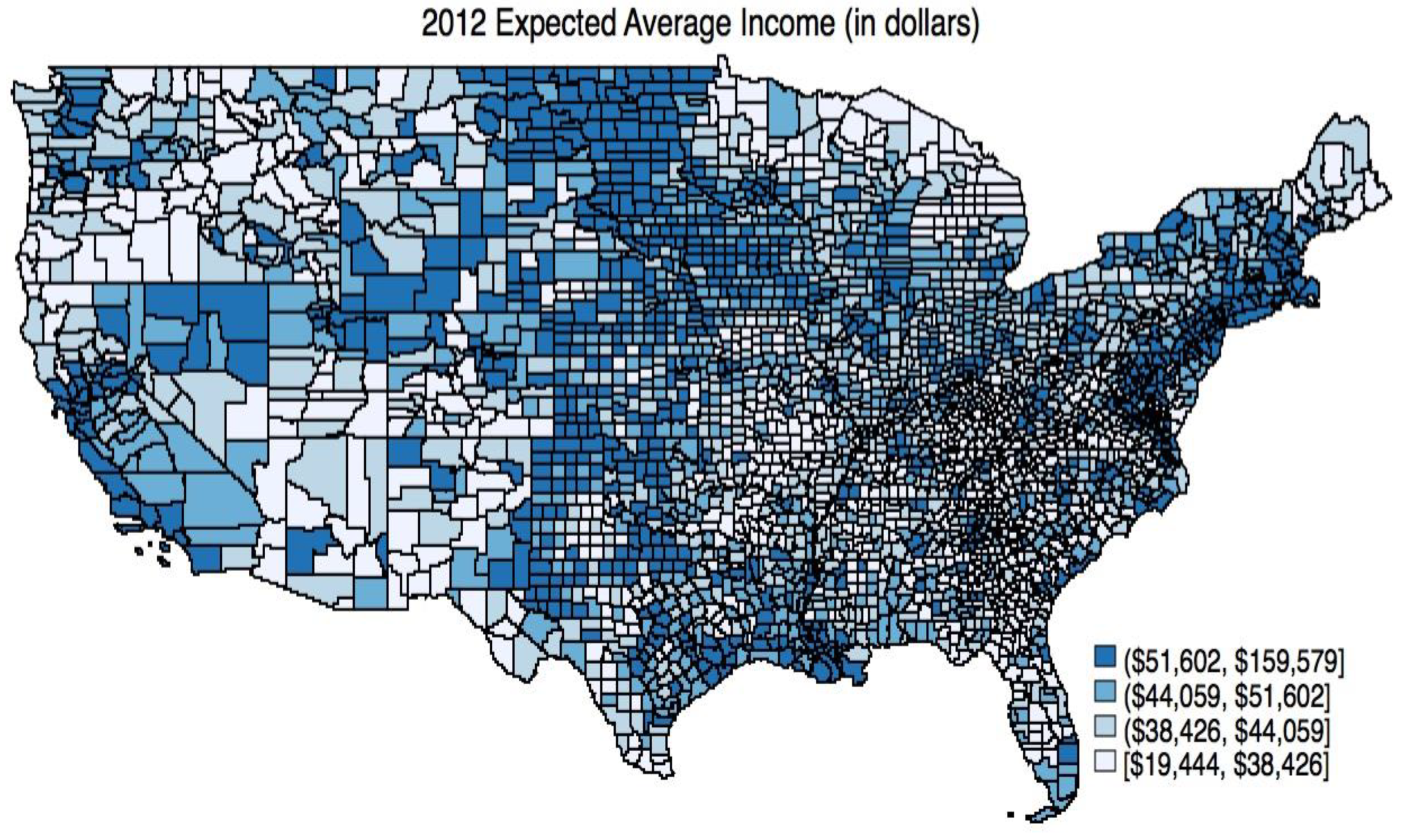
7.1. Expected Average Income

One of the dependent variables in this study, w, is defined as the expected average county income. The measure for w, as closely as possible, reflects earnings from local sources only. According to the underlying logic of the spatial hedonic model, people are willing to accept lower incomes if they can live in places that provide better amenities. The income that is relevant is that which they receive because they live in a particular place. Income that is unrelated to place (e.g., pension, retirement benefits, return on financial investments) does not affect their choices because they can obtain that income anywhere. The Bureau of Economic Analysis’ (BEA) personal income totals for each county are based on place of residence. Personal income is equal to the sum of net earnings by place of residence, property income (personal dividends, interest, and rental income), and current personal transfer receipts earned by the residents of each county. The ideal measure of income would not include personal interest income, dividends, rent, and most types of transfer receipts because these could be earned even if the individuals moved to another place. The BEA data on net earnings by place of residence 4 closely reflects the ideal measure, allowing us to exclude dividends, interest, rent, and personal current transfer receipts. The income that counts is wage income, business income (sole proprietorships and partnerships), and farm income (since 2004, the BEA has revised its income data to include the U.S. Department of Agriculture’s farm income data). In order to derive the net earnings by place-of-residence estimates, the BEA calculates a residence adjustment estimate for each county. Essentially, the procedure makes negative adjustments in areas that are work centers (most urban centers) and positive adjustments in suburban counties.

To calculate our final measure of variable w, we divide the BEA’s “net earnings by place-of-residence estimates” by the labor force by place of residence from the U.S. Bureau of Labor Statistics. This indicator of income implicitly includes the risk of being unemployed. For instance, if 5% of people in the labor force are unemployed, then the average person will expect to be unemployed 5% of the time, and our estimate of net earnings will reflect this.

Figure 2 shows the distribution of w across counties. Spatial patterns in Figure 1 indicate that darker colors represent higher values of the dependent variable, w. Expected average income has mean values of 46,677.61 for the nation, 511,180.93 for the metro, and 43,993.65 for the non-metro.

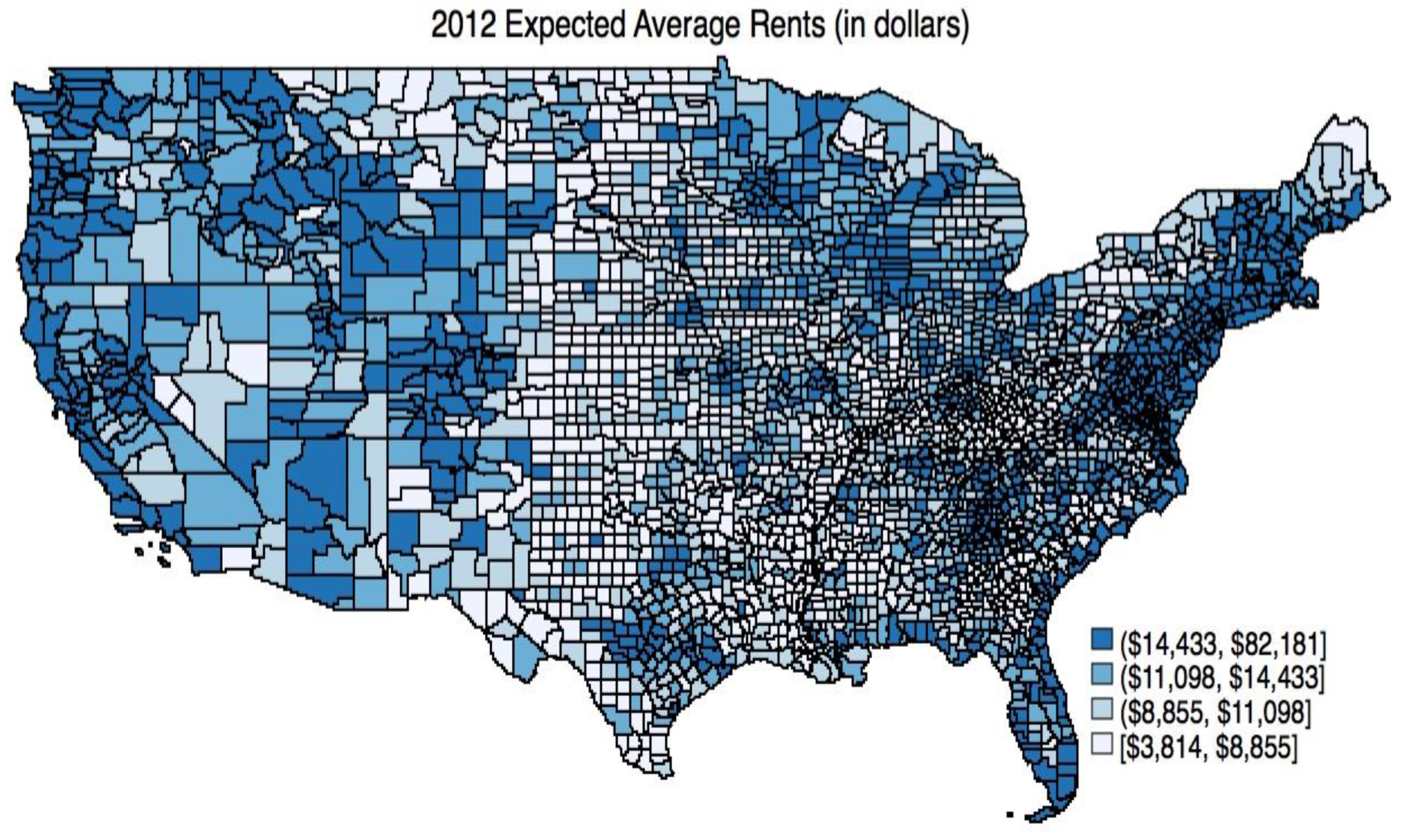
7.2. Expected Average Rent for Residential Sites

The economic rent of land is intended to be a measure of the variable r. This study defines r as expected average rents. This is based on a Ricardian rent concept and is equal to the value of unimproved land 5. Therefore, the amount that people pay to lease homes and the implicit value of owner-occupied dwellings is too high because it includes the value derived from the public and private improvements (buildings, street access, water service, etc.). Because the value of improvements is not equal in all locations, we need to separate the value of improvements from that of the land to accurately estimate the variable. Our county-based data, though not having the spatial specificity of the micro data used by Roback, include a broader range of residential sites than that of Roback (1982) [9] 6. We employ data on owner-occupied housing values from the American Community Survey in order to have comparable data for all 3109 counties 7.

To calculate the implicit price of an amenity as in Roback (1982) [9], housing values and earnings should be for the same time unit. The partial derivative of housing values with respect to an amenity includes the present value of all expected future benefits of owning the house, so here we translate housing values into annual rent. To calculate the rent, this study adapts the user cost method (Himmelberg et al., 2005 [29]; Poterba, 1984, 1992 [30,31]):

$$r=P \left[rf+\omega -\tau \left(rm+\omega \right)+{\delta }_t-{\gamma }_{t+1}+{\epsilon }_t\right],$$

(12)

where $P$ is the average county housing value 8; $rf$ is the risk-free interest rate; $\omega$ is the property tax rate; $\tau$ is the marginal income tax rate; $rm$ is the mortgage interest rate; ${\delta }_t$ is the depreciation rate; ${\gamma }_{t+1}$ is the expected capital gain rate; and ${\epsilon }_t$ is the owner’s risk premium.

The user cost method (Himmelberg et al., 2005 [29]; Poterba, 1984, 1992 [30,31]) estimates the real economic cost of homeownership in addition to the inclusion of direct payments for local public goods via property taxes (as cited in Bieri et al., 2023, p. 18 [32]), which can control the tax rates’ impact on the amenity (effects on land values) 9.

The risk-free rate is a 10-year average of 3-month Treasury bill rates and is set at $rf$= 0.045 (4.5%). This is the opportunity cost of money invested in the home. In addition, the mortgage rate is the 10-year average of the 30-year fixed-rate mortgage and is set at $rm$ = 0.055 and ${\delta }_t$ = 0.025. These values are based on estimates from Harding et al. (2007) [34].

We employed the 5-year average (2005–2009) of county property tax rates for the property tax rate ($\omega$; the most recent available), assuming that changes between the 2005–2009 average and 2012 have been proportional across jurisdictions. The national average annual property tax rate on owner-occupied housing is 0.97%. These data were obtained from the Tax Foundation (property taxes on owner-occupied housing, by county, 5-year average, 2005–2009; http://www.taxfoundation.org accessed on 9 November 2022.).

The term $\tau \left(rm+\omega \right)$ is the income tax savings to homeowners because mortgage interest ($rm$) and property taxes ($\omega$) are deductible from income for tax purposes. The income tax savings is subtracted from other costs because it is a benefit of home ownership.

Regarding the expected capital gain, we set average values of appreciation (40-year average rate of appreciation minus long-run inflation of 3.78% 10) at the state level, which indicates that the value varies across states (real estate appreciation data from http://www.estateofmindsites.com), whereas Bieri et al. (2023) [32] treated the expected capital gain as constant (${\gamma }_{t+1}$= 0.038, which was a long-run inflation of 2.0% plus a real appreciation of 1.8%). If homeowners maintain their homes in a constant physical condition (i.e., offset depreciation with repairs), the expected capital gain and appreciation rates are the same.

Figure 3 shows the distribution of expected average rents across counties. The darker colors in Figure 3 represent higher values of annual costs of housing consumption. It is interesting that the darker colored areas in Figure 1 match many of the light areas in Figure 2 in many areas, or vice versa. For instance, the middle band of the United States is visually distinct. This seems to support the idea that a place with higher amenities has relatively higher land values and lower wages, which is consistent with Roback’s (1982) [9] spatial equilibrium model. Expected average rents have mean values, of 12,498.28 for the nation, 15,293.33 for the metro, and 10,832.43 for the non-metro. More information on other variables (e.g., how to measure, sources, and descriptive statistics) is included in Appendix A.

8. Results: Non-Spatial vs. Spatial Models and Metro vs. Non-Metro Models

To employ spatial econometrics, we estimate equations for the entire continental United States because the spatial econometric models require spatial weights matrices to estimate the influence of neighboring counties, and thus dividing metro and non-metro counties into separate models is not possible.

We then employ the created contiguity-based spatial weight matrices from J. Kim et al. (2017) [26]. This study, thus, defines neighbors as counties having common borders (adjacent). At the same time, the model considers an endogenous variable in each equation. A dependent variable in one equation becomes a right-hand side variable in another equation.

We performed a Wald test on the estimated SAR coefficient ($\lambda$), and SAR models were statistically insignificant for both wage and rent equations. On the other hand, the estimated SEM coefficient ($\rho$) is positive and statistically significant, indicating spatial autocorrelation in the error term ($ϵ$). Therefore, this study reports results from the SEM model, which is preferable to the SAR model.

To test for differences in the marginal effects of the variables between metro and non-metro counties, we include a metro dummy variable and cross-products of the metro dummy with each of the variables. To implement 2SLS, we include all cross-products of each of the explanatory variables in the second stage. However, we need to consider interaction terms for the predicted endogenous variable in the second stage and thus each equation is assumed to have two endogenous variables (e.g., log county income and metro $\times$ log county income) and other excluded instruments, which consist of all instrumental variables and all cross-products of the metro dummy with each of the instrumental variables.

This section describes the SEM 2SLS with an assumption of normality of the error term. The spatial econometric model in this study assumes the term ϵ in the specification of the equation to be independent and identically distributed (IID) or independent but heteroskedastically distributed, where the heteroskedasticity is an unknown form (see Drukker et al., 2011, 2013 [27,28]). We implemented both cases of homoskedastic and heteroskedastic specification in the econometric models and the results were identical, except for the spatial autoregressive parameters for both wage and rent equations. The spatial autoregressive parameters in the heteroskedastic specification were slightly higher than the values in the homoskedastic specification 11. Both specifications produced consistent estimates from the pretesting. Thus, we only report estimates from SEM 2SLS with an assumption of IID ϵ.

Table 1. Direct marginal effects for rent equations: non-spatial versus spatial models in the continental United States.

	Metro		Non-metro
Variable	Non-Spatial 2SLS Rent	Spatial 2SLS Rent	Non-Spatial 2SLS Rent	Spatial 2SLS Rent
Log County Income	$-$0.23	$-$0.83 $\times {10}^{-1}$	$-$0.25	$-$0.25
County Revenue	0.22 $\times {10}^{-1}$	0.12 $\times {10}^{-1}$	0.31 $\times {10}^{-2}$	0.31 $\times {10}^{-2}$
Land Share	0.61 $\times {10}^1$	0.67 $\times {10}^1$	0.73 $\times {10}^1$	0.73 $\times {10}^1$
County Population	0.50 $\times {10}^{-7}$	0.40 $\times {10}^{-7}$	0.15 $\times {10}^{-5}$	0.12 $\times {10}^{-5}$
High School Graduation	0.52 $\times {10}^{-3}$	0.42 $\times {10}^{-3}$	0.11 $\times {10}^{-3}$	0.23 $\times {10}^{-3}$
Extreme Temp	$-$0.42 $\times {10}^{-4}$	$-$0.26 $\times {10}^{-4}$	$-$0.23 $\times {10}^{-4}$	$-$0.18 $\times {10}^{-4}$
PM 2.5	$-$0.71 $\times {10}^{-2}$	$-$0.40 $\times {10}^{-2}$	$-$0.42 $\times {10}^{-2}$	$-$0.26 $\times {10}^{-2}$
County Violent Crime	$-$0.36 $\times {10}^{-4}$	$-$0.67 $\times {10}^{-5}$	0.37 $\times {10}^{-4}$	0.39 $\times {10}^{-4}$
County GINI	0.69	0.30	$-$0.74 $\times {10}^{-1}$	$-$0.15
Mammography	0.11 $\times {10}^{-2}$	0.12 $\times {10}^{-2}$	0.11 $\times {10}^{-2}$	0.79 $\times {10}^{-3}$
Physical Activity	0.18 $\times {10}^{-2}$	0.11 $\times {10}^{-2}$	0.39 $\times {10}^{-3}$	0.39 $\times {10}^{-3}$
Child Poverty	$-$0.13 $\times {10}^{-1}$	$-$0.66 $\times {10}^{-2}$	$-$0.96 $\times {10}^{-2}$	$-$0.78 $\times {10}^{-2}$

Note. The values are based on Table A13 (see Appendix A). See Appendix A for all other variables’ information.

presents estimated coefficients based on the second-stage coefficients, which are estimates of the structural parameters. The coefficients indicate the direct effects of independent variables. Including spatial interactions produce slightly different direct marginal effects compared with non-spatial models for metro counties. Non-metro counties have very similar marginal effect values between spatial and non-spatial models. For metro counties, the inclusion of spatial effects decreases the directs effects of violent crime and child poverty, which implies that people in metro counties prefer places with less violence and less child poverty. For physical activity, both equations for metro and non-metro counties have positive effects on rent. The inclusion of spatial effects decreases slightly the direct marginal effect of physical activity opportunities in both metro and non-metro counties.

Table 2. Total marginal effects for rent equations in the continental United States: metro versus non-metro and non-spatial versus spatial models.

Rent Equation	Non-Spatial Model		Spatial Model
Variable	Non-Metro	Metro	Non-Metro	Metro
County Revenue	0.35 $\times {10}^{-2}$	0.12 $\times {10}^{-1}$	0.34 $\times {10}^{-2}$	0.92 $\times {10}^{-2}$
Land Share	0.74 $\times {10}^1$	0.60 $\times {10}^1$	0.74 $\times {10}^1$	0.66 $\times {10}^1$
County Violent Crime	0.15 $\times {10}^{-4}$	$-$0.39 $\times {10}^{-4}$	0.20 $\times {10}^{-4}$	$-$0.14 $\times {10}^{-4}$
Private Public School	0.13 $\times {10}^{-2}$	0.13 $\times {10}^{-2}$	0.71 $\times {10}^{-3}$	0.12 $\times {10}^{-2}$
County GINI	$-$0.44	0.97 $\times {10}^{-1}$	$-$0.39	$-$0.76 $\times {10}^{-2}$
Child Poverty	$-$0.82 $\times {10}^{-2}$	$-$0.11 $\times {10}^{-1}$	$-$0.63 $\times {10}^{-2}$	$-$0.73 $\times {10}^{-2}$
Physical Activity	0.45 $\times {10}^{-3}$	0.14 $\times {10}^{-2}$	0.47 $\times {10}^{-3}$	0.82 $\times {10}^{-3}$
High School Graduation	0.24 $\times {10}^{-3}$	0.64 $\times {10}^{-3}$	0.29 $\times {10}^{-3}$	0.41 $\times {10}^{-3}$
Poor Water Quality	0.31 $\times {10}^{-4}$	$-$0.52 $\times {10}^{-4}$	0.32 $\times {10}^{-4}$	$-$0.30 $\times {10}^{-3}$
Mammography	0.10 $\times {10}^{-2}$	0.13 $\times {10}^{-2}$	0.58 $\times {10}^{-3}$	0.11 $\times {10}^{-2}$
Extreme Temp	$-$0.18 $\times {10}^{-4}$	$-$0.46 $\times {10}^{-4}$	$-$0.13 $\times {10}^{-4}$	$-$0.34 $\times {10}^{-4}$
Sunshine	0.12 $\times {10}^{-2}$	0.18 $\times {10}^{-5}$	0.13 $\times {10}^{-2}$	0.78 $\times {10}^{-3}$
PM 2.5	$-$0.18 $\times {10}^{-2}$	$-$0.71 $\times {10}^{-2}$	$-$0.90 $\times {10}^{-3}$	$-$0.44 $\times {10}^{-2}$
County Unemployment	0.92 $\times {10}^{-3}$	0.10 $\times {10}^{-1}$	0.10 $\times {10}^{-2}$	0.48 $\times {10}^{-2}$
County Population	0.15 $\times {10}^{-5}$	0.50 $\times {10}^{-7}$	0.12 $\times {10}^{-5}$	0.30 $\times {10}^{-7}$
Population Growth	0.14 $\times {10}^{-2}$	0.23 $\times {10}^{-2}$	$-$0.99 $\times {10}^{-3}$	0.40 $\times {10}^{-2}$

Note. The values of the marginal effects are based on Table 1.

,

Table 3. Direct marginal effects for wage equations: non-spatial versus spatial 2SLS in the continental United States.

	Metro		Non-Metro
Variable	Non-Spatial 2SLS Wage	Spatial 2SLS Wage	Non-Spatial 2SLS Wage	Spatial 2SLS Wage
Log County Rent	0.61	0.55	0.43	0.33
County Revenue	0.42 $\times {10}^{-2}$	0.21 $\times {10}^{-2}$	0.47 $\times {10}^{-2}$	0.97 $\times {10}^{-3}$
Land Share	$-$0.36 $\times {10}^1$	$-$0.26 $\times {10}^1$	$-$0.42 $\times {10}^1$	$-$0.28 $\times {10}^1$
County Unemployment	$-$0.15 $\times {10}^{-1}$	$-$0.13 $\times {10}^{-1}$	$-$0.16 $\times {10}^{-1}$	$-$0.14 $\times {10}^{-1}$
Population Growth	$-$0.49 $\times {10}^{-2}$	$-$0.25 $\times {10}^{-2}$	0.10 $\times {10}^{-1}$	0.11 $\times {10}^{-1}$
Private Public School	0.19 $\times {10}^{-2}$	0.19 $\times {10}^{-2}$	0.74 $\times {10}^{-3}$	0.45 $\times {10}^{-3}$
Sunshine	$-$0.30 $\times {10}^{-2}$	$-$0.29 $\times {10}^{-2}$	0.28 $\times {10}^{-3}$	0.43 $\times {10}^{-3}$
County GINI	0.80	0.66	0.42	0.40
Poor Water Quality	0.75 $\times {10}^{-3}$	0.59 $\times {10}^{-3}$	$-$0.28 $\times {10}^{-3}$	$-$0.30 $\times {10}^{-3}$
Mammography	$-$0.17 $\times {10}^{-2}$	$-$0.16 $\times {10}^{-2}$	0.16 $\times {10}^{-2}$	0.20 $\times {10}^{-2}$

Note. The values are based on Table A15 (see Appendix A).

and

Table 4. Total marginal effects for wage equations in the continental United States: metro versus non-metro.

Rent Equation	Non-Spatial Model		Spatial Model
Variable	Non-Metro	Metro	Non-Metro	Metro
County Revenue	0.12 $\times {10}^{-2}$	0.84 $\times {10}^{-2}$	$-$0.28 $\times {10}^{-3}$	0.75 $\times {10}^{-2}$
Land Share	$-$0.78	0.25	$-$0.44	0.66
County Violent Crime	0.84 $\times {10}^{-4}$	0.38 $\times {10}^{-4}$	0.69 $\times {10}^{-4}$	0.21 $\times {10}^{-4}$
Private Public School	0.89 $\times {10}^{-3}$	0.32 $\times {10}^{-2}$	0.51 $\times {10}^{-3}$	0.27 $\times {10}^{-2}$
County GINI	0.10 $\times {10}^1$	0.15 $\times {10}^1$	0.79	0.13 $\times {10}^1$
Child Poverty	$-$0.99 $\times {10}^{-2}$	$-$0.12 $\times {10}^{-1}$	$-$0.86 $\times {10}^{-2}$	$-$0.10 $\times {10}^{-1}$
Physical Activity	0.22 $\times {10}^{-3}$	$-$0.44 $\times {10}^{-5}$	0.14 $\times {10}^{-3}$	0.50 $\times {10}^{-4}$
High School Graduation	0.14 $\times {10}^{-3}$	0.80 $\times {10}^{-3}$	0.42 $\times {10}^{-4}$	0.55 $\times {10}^{-3}$
Poor Water Quality	0.21 $\times {10}^{-4}$	0.67 $\times {10}^{-3}$	$-$0.15 $\times {10}^{-3}$	0.38 $\times {10}^{-3}$
Mammography	0.13 $\times {10}^{-2}$	$-$0.13 $\times {10}^{-2}$	0.12 $\times {10}^{-2}$	$-$0.93 $\times {10}^{-3}$
Extreme Temp	0.52 $\times {10}^{-5}$	0.17 $\times {10}^{-4}$	0.77 $\times {10}^{-5}$	$-$0.18 $\times {10}^{-4}$
Sunshine	0.31 $\times {10}^{-2}$	$-$0.19 $\times {10}^{-2}$	0.33 $\times {10}^{-2}$	$-$0.19 $\times {10}^{-2}$
PM 2.5	$-$0.33 $\times {10}^{-2}$	$-$0.28 $\times {10}^{-2}$	$-$0.36 $\times {10}^{-2}$	$-$0.27 $\times {10}^{-2}$
County Unemployment	0.21 $\times {10}^{-2}$	0.67 $\times {10}^{-2}$	0.87 $\times {10}^{-3}$	0.30 $\times {10}^{-2}$
County Population	0.59 $\times {10}^{-6}$	0.16 $\times {10}^{-7}$	0.40 $\times {10}^{-6}$	0.11 $\times {10}^{-7}$
Population Growth	0.99 $\times {10}^{-2}$	$-$0.27 $\times {10}^{-2}$	0.98 $\times {10}^{-2}$	$-$0.33 $\times {10}^{-2}$

Note. The values of the marginal effects are based on Table A16 (see Appendix A).

below present estimated coefficients and calculated marginal effects for metro and non-metro for non-spatial and spatial models based on the reduced-form coefficients, which are estimates of the total (direct and indirect) effects of each of the variables. In Table 2, we see a decreased magnitude gap for county revenues between metro and non-metro counties when including spatial interactions.

Child poverty, high school graduation rates, extreme temperature, and PM 2.5 have unexpected signs for the full implicit price. Large negative wage effects of child poverty and PM 2.5 outweigh the impacts on property values. Enhanced environmental policies affecting firms in metro counties might increase the costs of production. The higher human capital stock also might increase firms’ costs in metro counties.

In

Table 5. Annualized values based on non-spatial and spatial models for the metro.

	Annualized Value
Variable	Rent Equation		Wage Equation		Full Implicit Price
	Non-Spatial	Spatial	Non-Spatial	Spatial	Non-Spatial	Spatial
County Revenue (thousands of dollars per capita)	61.10	47.14	429.41	385.77	$-$368.32	$-$338.62
Land Share (fraction to consumer budget)	30,900.19	33,851.50	13,025.22	33,533.65	17,874.98	317.85
County Violent Crime (violent crimes/100,000 population)	$-$0.20	$-$0.07	1.93	1.07	$-$2.13	$-$1.14
Private Public School (fraction)	6.56	6.38	161.96	138.49	$-$155.40	$-$132.11
County GINI (index)	497.34	$-$38.97	78,655.21	66,045.64	$-$78,157.87	$-$66,084.60
Child Poverty (% children in poverty)	$-$56.52	$-$37.37	$-$602.36	$-$520.57	545.84	483.20
Physical Activity (% pop. with access to physical activity places)	7.21	4.19	$-$0.23	2.53	7.44	1.66
High School Graduation (% of graduation rate)	3.25	2.11	41.08	28.10	$-$37.83	$-$25.99
Poor Water Quality (% pop. in water violation)	$-$0.26	$-$1.56	34.10	19.35	$-$34.36	$-$20.91
Mammography (% female Medicare enrollees)	6.41	5.55	$-$64.7	$-$47.64	70.98	53.20
Extreme Temp (1 °F colder for one day)	$-$0.24	$-$0.17	$-$0.86	$-$0.91	0.62	0.74
Sunshine (% of possible)	0.01	3.98	−98.07	$-$97.24	98.08	101.22
PM 2.5 (µg/m3)	$-$36.29	$-$22.55	$-$141.93	$-$136.41	105.64	113.86
County Unemployment (fraction of unemployment)	53.48	24.54	342.31	153.58	$-$288.83	$-$129.04
County Population (10,000 persons)	2.56	1.54	8.19	5.63	$-$5.63	$-$4.09
Population Growth (percentage change in pop.)	11.75	20.66	$-$136.24	$-$169.61	147.99	190.27

Note. Annualized value is in dollars. Measurement units of amenities are shown under variable names. Each entry is computed and evaluated at mean annual county income as follows: $P_s^{*}$ = $(k_l\frac{d \log r}{ds}$$-$$\frac{d\log w}{ds})w$. The average land share of the consumer’s budget ($k_l$) is 0.01 for the metro. The average annual expected income ($w$) is $51,180.93 for the metro.

, the inclusion of spatial interactions decreased the magnitude of the full implicit prices of both county GINI and violent crime. Conceptually, unequal distribution of income (county GINI) could have a positive or negative effect on property values. One would expect that it would be a disamenity to most residents, but if the unequal distribution leads to more property ownership by the richer segments of society, it could increase rent levels. The implicit values for county GINI are very high, but it is important to remember that this variable has potential values between 0 (perfect equality) and 1.0 (perfect inequality). Given that most of our observations are between 0.35 and 0.55, the actual differences between communities are only a fraction of this value.

Table 6. Annualized values based on non-spatial and spatial models for the non-metro.

	Annualized Value
Variable	Rent Equation		Wage Equation		Full Implicit Price
	Non-Spatial	Spatial	Non-Spatial	Spatial	Non-Spatial	Spatial
County Revenue (thousands of dollars per capita)	11.59	11.15	53.39	$-$12.23	$-$41.80	23.38
Land Share (fraction to consumer budget)	24,307.93	24,271.69	$-$34,182.32	$-$19,230.98	58,490.25	43,502.67
County Violent Crime (violent crimes/100,000 population)	0.05	0.07	3.70	3.01	$-$3.65	$-$2.95
Private Public School (fraction)	4.31	2.33	39.31	22.30	$-$35.00	$-$19.97
County GINI (index)	$-$1459.08	$-$1280.84	44,498.96	34,632.02	$-$45,958.04	$-$35,912.86
Child Poverty (% children in poverty)	$-$27.14	$-$20.80	$-$433.76	$-$378.58	406.62	357.78
Physical Activity (% pop. with access to physical activity places)	1.48	1.55	9.58	6.05	$-$8.10	$-$4.49
High School Graduation (% of graduation rate)	0.79	0.94	6.17	1.85	$-$5.39	$-$0.90
Poor Water Quality (% pop. in water violation)	0.10	0.10	0.92	$-$6.78	$-$0.81	6.88
Mammography (% female Medicare enrollees)	3.44	1.91	58.23	54.69	$-$54.79	$-$52.78
Extreme Temp (1 °F colder for one day)	$-$0.06	$-$0.04	0.23	0.34	$-$0.29	$-$0.38
Sunshine (% of possible)	3.87	4.26	138.39	143.52	$-$134.52	$-$139.26
PM 2.5 (µg/m3)	$-$6.04	$-$2.97	$-$143.15	$-$157.03	137.11	154.06
County Unemployment (fraction of unemployment)	3.04	3.39	94.28	38.32	$-$91.24	$-$34.93
County Population (10,000 persons)	48.17	39.26	261.41	173.83	$-$213.23	$-$134.57
Population Growth (percentage change in pop.)	4.63	$-$3.28	435.16	432.87	$-$430.53	$-$436.15

Note. Annualized value is in dollars. Measurement units of amenities are shown under variable names. Each entry is computed and evaluated at mean annual county income as follows: $P_s^{*}$ = $(k_l\frac{d \log r}{ds}$$-$$\frac{d\log w}{ds})w$. The average land share of the consumer’s budget ($k_l$) is 0.075 for non-metro counties. The average annual expected income ($w$) is $43,993.65 for non-metro counties.

shows that, as in metro counties, including spatial interactions in the non-metro model decreased the magnitude of the full implicit prices for both county GINI and violent crime. For county revenue, including spatial interactions made the positive wage effects negative, and thus there was a positive full implicit price, which indicates that g is underprovided. PM 2.5 has an unexpected positive value for the full implicit price due to the large negative wage effect.

9. Concluding Remarks

The model employed in this study helps us understand the underlying forces driving spatial variations in land values and wages. Our findings indicate that changing property values are not simply an issue of supply and typical demand variables but also indicate changes in the level and demand for amenities. This suggests different policy strategies. For example, rising property values due to improving built amenities is a justification for funding these public investments with property taxes rather than other sources of revenue. Lower housing affordability (i.e., higher land prices relative to wages) is generally viewed as a negative. However, these results show that rising housing prices are sometimes an equilibrium response to the rising level of, or increased demand for amenities, which signals an increasing comprehensive wealth of residents. In the opposite case, declining housing costs, while making housing more affordable, is not necessarily desirable if it is due to the declining quality of natural and publicly provided amenities. The results of this study also help us understand the feedback and spillover effects of changing amenities on wages and land values in neighboring counties.

There are apparently differences between the value of amenities in metro and non-metro counties. Violent crime and unequal distribution of income were disamenities. For county GINI, larger positive wage effects in metro counties produced larger negative full implicit value than in non-metro counties. For county revenue, the full implicit value indicated that government services are overprovided in metro (negative value) but are underprovided in non-metro counties (positive value) in the spatial model specifications.

The general spatial equilibrium model yields strong implications for measuring comprehensive wealth by linking the value of nonmarketed immobile local amenities and local land rents and wages and by partitioning values attributable to various types of capital. Many intangible and nonmarketable assets increase the value of tangible market assets, such as land. On the basis of this model, increasing income is associated with an increased level of nonmarketed immobile local amenities, which can make wealth more sustainable. The results of this study contribute to the research literature by refining the indicators of local income, land rent, and amenities, which can contribute natural, social, and human capital to the wealth of a location.

Additionally, this study introduces several modifications to the Roback framework. We estimated an SDEM for all 3109 counties in the contiguous United States with aggregate county-level data that allowed the full range of advantages of spatial analysis. Including interactions between a metro dummy and each explanatory variable in the pooled regression allowed us to estimate distinct coefficients for metro and non-metro counties. Furthermore, this study effectively separates the effects of local and nearby amenities using spatial econometric methods. The model produces mostly expected results with relatively high R-squared values for a cross-sectional model.

There are important policy implications for this research. The results provide estimates of the relative value of various local assets and amenities, providing policymakers with a stronger basis for allocating public funding. On the basis of the empirical results, policymakers should view policies designed to reduce crime rates and income inequality as elements of their economic development toolbox. Results also indicate that policymakers must consider their spatial context and expect spatial interactions with neighboring counties. In particular, the spatial lag of cross-products of the metro dummy with violent crime indicates that a metro county’s violent crime rate decreases land values and the comprehensive wealth of residents of neighboring counties. This should encourage localities to collaborate and coordinate their efforts. The same levels of amenities have different impacts on land values and wages depending on the levels of these amenities in adjacent counties. Well-designed policies and investments in immobile and nonmarketed amenities of a location will make a place more attractive and sustainable with enhanced land values, which contributes to balancing place prosperity and people prosperity.

In conclusion, spatial analysis of the value of place-specific natural, cultural, social, and publicly provided amenities and assets moves us one step closer to our goal of accurately measuring the level of, and changes in, comprehensive wealth at the local level and ultimately to public policy strategies available to enhance societal comprehensive wealth and sustainability.

References

1. Arrow, K.J.; Dasgupta, P.; Goulder, L.H.; Mumford, K.J.; Oleson, K. Sustainability and the measurement of wealth. Environ. Dev. Econ. 2012, 17, 317–353. [Google Scholar] [CrossRef]
2. Cobb, C.W.; Daly, H. The index of sustainable economic welfare. In For the Common Good: Redirecting the Economy toward Community, the Environment, and a Sustainable Future; Daly, H.E., Cobb, J.B., Eds.; Beacon Press: Boston, MA, USA, 1989. [Google Scholar]
3. Pender, J.L.; Weber, B.A.; Johnson, T.G.; Fannin, J.M. (Eds.) Rural Wealth Creation; Routledge: Oxfordshire, UK, 2014. [Google Scholar]
4. United Nations University–International Human Dimensions Programme and United Nations Environment Programme. Inclusive Wealth Report 2014: Measuring Progress Toward Sustainability; Cambridge University Press: Cambridge, UK, 2014. [Google Scholar]
5. World Bank. Where Is the Wealth of Nations? Measuring Capital for the 21st Century; World Bank: Washington, DC, USA, 2006. [Google Scholar]
6. World Bank. The Changing Wealth of Nations. Measuring Sustainable Development in the New Millennium; World Bank: Washington, DC, USA, 2011. [Google Scholar]
7. Nordhaus, W.D. How Should We Measure Sustainable Income? Cowles Foundation Discussion Paper No. 1101; Yale University, Cowles Foundation for Research in Economics: New Haven, CT, USA, 1995. [Google Scholar]
8. Nordhaus, W.D. New directions in national economic accounting. Am. Econ. Rev. 2000, 90, 259–263. [Google Scholar] [CrossRef]
9. Roback, J. Wages, rents, and the quality of life. J. Political Econ. 1982, 90, 1257–1278. [Google Scholar] [CrossRef]
10. Partridge, M.D.; Rickman, D.S.; Olfert, M.R.; Tan, Y. When spatial equilibrium fails: Is place-based policy second best? Reg. Stud. 2015, 49, 1303–1325. [Google Scholar] [CrossRef]
11. Evans, A.W. The assumption of equilibrium in the analysis of migration and interregional differences: A review of some recent research. J. Reg. Sci. 1990, 30, 515–531. [Google Scholar] [CrossRef] [PubMed]
12. Greenwood, M.J.; Hunt, G.L.; Rickman, D.S.; Treyz, G.I. Migration, regional equilibrium, and the estimation of compensating differentials. Am. Econ. Rev. 1991, 81, 1382–1390. [Google Scholar]
13. Rappaport, J. Moving to nice weather. Reg. Sci. Urban Econ. 2007, 37, 375–398. [Google Scholar] [CrossRef]
14. Mueser, P.R.; Graves, P.E. Examining the role of economic opportunity and amenities in explaining population redistribution. J. Urban Econ. 1995, 37, 176–200. [Google Scholar] [CrossRef]
15. Putnam, R. Social capital: Measurement and consequences. Can. J. Policy Res. 2001, 2, 41–51. [Google Scholar]
16. Daly, H.E. Steady-State Economics: Second Edition with New Essays; Island Press: Washington, DC, USA, 1991. [Google Scholar]
17. Wu, J.; Gopinath, M. What causes spatial variations in economic development in the United States? Am. J. Agric. Econ. 2008, 90, 392–408. [Google Scholar] [CrossRef]
18. Deller, S.C.; Tsai, T.H.; Marcouiller, D.W.; English, D.B. The role of amenities and quality of life in rural economic growth. Am. J. Agric. Econ. 2001, 83, 352–365. [Google Scholar] [CrossRef]
19. Osei, M.J.; Winters, J.V. Labor demand shocks and housing prices across the United States: Does one size fit all? Econ. Dev. Q. 2019, 33, 212–219. [Google Scholar] [CrossRef]
20. Rappaport, J.; Sachs, J.D. The United States as a coastal nation. J. Econ. Growth 2003, 8, 5–46. [Google Scholar] [CrossRef]
21. Frank, R.H. Choosing the Right Pond: Human Behavior and the Quest for Status; Oxford University Press: New York, NY, USA, 1985. [Google Scholar]
22. Smith, V.K. Residential location and environmental amenities: A review of the evidence. Reg. Stud. 1977, 11, 47–61. [Google Scholar] [CrossRef]
23. Baum, C.F. An Introduction to Modern Econometrics Using Stata; Stata Press: College Station, TX, USA, 2006. [Google Scholar]
24. Wooldridge, J. Econometric Analysis of Cross Section and Panel Data; MIT Pres: Cambridge, MA, USA, 2002. [Google Scholar]
25. Wooldridge, J.M. Introductory Econometrics, a Modern Approach; Thomson/South-Western: Mason, OH, USA, 2006. [Google Scholar]
26. Kim, J.; Johnson, T.; Pender, J. Revisiting Roback’s Spatial Hedonic Equilibrium Model: A County-Level Analysis with an Explicit Spatial approach. In Proceedings of the 2017 Southern Regional Science Association Conference, Memphis, TN, USA, 1 April 2017. [Google Scholar]
27. Drukker, D.M.; Prucha, I.R.; Raciborski, R. Maximum Likelihood and Generalized Spatial Two-Stage Least-Squares Estimators for a Spatial-Autoregressive Model with Spatial-Autoregressive Disturbances; University of Maryland, Department of Economics: College Park, MA, USA, 2011. [Google Scholar]
28. Drukker, D.M.; Peng, H.; Prucha, I.R.; Raciborski, R. Creating and managing spatial-weighting matrices with the spmat command. Stata J. 2013, 13, 242–286. [Google Scholar] [CrossRef]
29. Himmelberg, C.; Mayer, C.; Sinai, T. Assessing high house prices: Bubbles, fundamentals and misperceptions. J. Econ. Perspect. 2005, 19, 67–92. [Google Scholar] [CrossRef]
30. Poterba, J.M. Tax subsidies to owner-occupied housing: An asset-market approach. Q. J. Econ. 1984, 99, 729–752. [Google Scholar] [CrossRef]
31. Poterba, J.M. Taxation and Housing: Old Questions, New Answers; Working Paper No. 3963; National Bureau of Economic Research (NBER): Cambridge, MA, USA, 1992. [Google Scholar]
32. Bieri, D.S.; Kuminoff, N.V.; Pope, J.C. National Expenditures on Local Amenities. J. Environ. Econ. Manag. 2023, 117, 102717. Available online: https://www.sciencedirect.com/science/article/abs/pii/S0095069622000766 (accessed on 1 February 2023). [CrossRef]
33. Oates, W.E. The effects of property taxes and local public spending on property values: An empirical study of tax capitalization and the Tiebout hypothesis. J. Political Econ. 1969, 77, 957–971. [Google Scholar] [CrossRef]
34. Harding, J.P.; Rosenthal, S.S.; Sirmans, C.F. Depreciation of housing capital, maintenance, and house price inflation: Estimates from a repeat sales model. J. Urban Econ. 2007, 61, 193–217. [Google Scholar] [CrossRef]
Figure 1. Conceptual logic: sources of social amenities from public investments.
Land 12 00586 g001
Figure 2. Expected average income for counties in the continental United States. Source: created by the authors using STATA software.
Land 12 00586 g002
Figure 3. Expected average rents for counties in the continental United States. Source: created by the authors using STATA software.
Land 12 00586 g003