Topography, Soil Elemental Stoichiometry and Landscape Structure Determine the Nitrogen and Phosphorus Loadings of Agricultural Catchments in the Subtropics

Abstract

The control of nitrogen (N) and phosphorus (P) loadings to receiving waters is often overcompensated for by catchment planners. The objectives of this study, which investigated nine catchments in the subtropics of China, were to (i) quantify the explicit relationships between the N and P loadings to receiving waters and the topographic, soil and landscape characteristics of catchments, (ii) identify key impact factors and (iii) identify the most influential N and P loading pathways via catchments. Our collective data indicated that elevation–relief ratio, soil elemental stoichiometry and landscape structure determined the N and P loadings of the studied agricultural catchments. The N export from catchments characterized by a woodland backdrop (Masson pine) mosaic with the intrusion of paddy fields in the subtropics was postulated to be driven by two simultaneous processes: discharge and retention. In addition, a soil C:P threshold ratio for the catchment N and P loadings was estimated to be in the range of 107–117. Our PLS-SEM path analyses suggested that to reduce the N export from agricultural catchments in the subtropics, mitigation practices in landscape ecosystems (e.g., landscape patterns, ditches and streams) need to be taken into consideration and predominantly deployed, despite traditional measures used for soils. Strategies to lower the catchment P export can be directly proposed at the source site. Our findings provide greater insights into the transport and retention of N and P nutrients through catchments and may optimally direct the focus of catchment planners, thus increasing the control efficacy of catchment N and P losses.

1. Introduction

Successful catchment water quality management relies on a clear theoretical understanding of how driving forces impact stream water quality. Globally, in terrestrial ecosystems, climate, atmospheric deposition, topography/hydrology, geology/soil type and land use (land cover and land management) are the key factors affecting nutrient (e.g., nitrogen–N, phosphorus–P) loadings to receiving waters [1,2,3,4]. Zooming into the catchment scale (up to 1000 km² in area), the nutrient loadings are related to topography, soil properties and land use types, particularly the latter two when the nutrient loadings are weighted by catchment runoff. Topographical characteristics of catchments (e.g., area, elevation and slope) strongly affect catchment hydrology and stream water quality, e.g., [5,6,7]. Numerous studies have shown that land use types, or the landscape composition of catchments, can impact the stream water quality or the N and P loadings to receiving waters, e.g., [8,9,10,11,12,13,14,15,16]. The spatial arrangement of land uses or the landscape configuration within catchments has also been shown to influence N and P concentrations in stream water, but this is less studied than the landscape composition [2,10,11,15,17,18]. The landscape configuration metrics are expected to better account for the hydrologic connectivity, nutrient loading quantity and flow path between nutrient sources and streams [3,4,19]. However, as an important medium of N and P sources, sinks and transport at the catchment level, soil’s properties, including elemental stoichiometric ratios, are rarely investigated in relation to the N and P loadings receiving stream waters, except in terms of chemical characteristics [20], erodibility [21] and drainage capacity [22]. Furthermore, the hierarchical relationships (or pathways) between topography, soil and landscape with respect to controlling the N and P loadings to receiving stream waters remain unclear and new techniques should be explored.

Structural equation modeling (SEM) is a statistical method (a combination of variance, co-variance, correlation, regression, factor and path analyses) that is widely used by researchers in the social, behavioral, educational, management and ecological sciences for the investigation of causal relationships [23,24]. SEM is a useful tool for environmentalists and ecologists, allowing them to study the causal relationships of N and P loadings versus environmental factors (e.g., topography, soil and landscape) at the catchment scale. There are two types of SEMs: conventional covariance-based SEM (CB-SEM) and variance-based partial least squares SEM (PLS-SEM); they make different data distributional assumptions and have different objectives. Using the maximum likelihood (ML) estimation method, which implies a multivariate normal distribution, CB-SEM aims to estimate model parameters so that the discrepancy between the model implied and sample covariance matrices is minimized. On the other hand, PLS-SEM, originally developed by Wold [25] and Lohmoeller [26], aims to maximize dependent variables’ explained variance by adopting an ordinary least squares estimation method. PLS-SEM is a nonparametric method that makes no data distributional assumption. It is primarily used to develop theories in exploratory research. Where the ML assumptions are hard to meet, PLS-SEM provides a good solution. According to Hair et al. [27], PLS-SEM is advantageous over CB-SEM in situations in which sample sizes are small, the data are not normally distributed, and complex models with many observed variables and relationships are estimated.

In this paper, we investigated nine agricultural catchments in the subtropics and examined the relationships of the N and P loadings to receiving waters with three environmental factors: topography, landscape and soil. We also detected the significant pathways of the catchment N and P loadings to receiving waters via soil and landscape by deploying the PLS-SEM method for N and P water pollution control. The outcomes of our study have the potential to provide deep insights into the transport and retention processes of N and P biogeochemical cycles at the catchment scale.

2. Materials and Methods

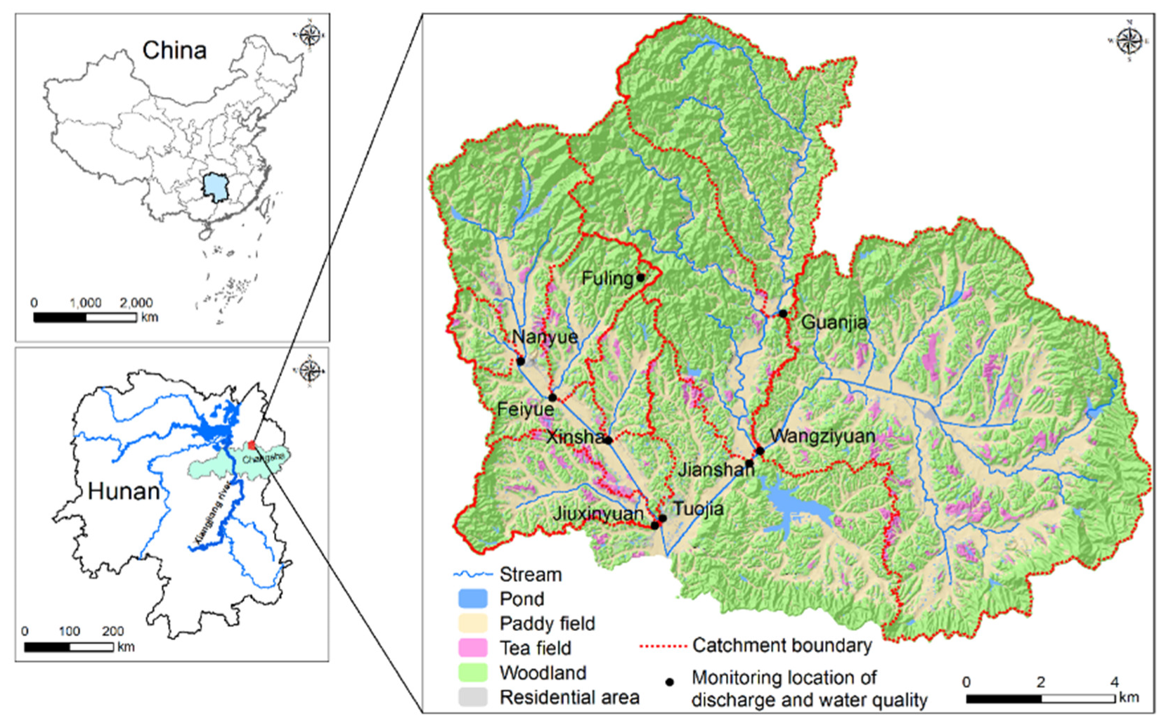
2.1. Study Area

The study area (135 km²) is a naturally formed catchment located at the Changsha Research Station for Agricultural & Environmental Monitoring (27°55′–28°40′ N, 112°56′–113°30′ E, elevation of 46–452 m) of the Chinese Academy of Sciences (CAS) in the Hunan Province (Figure 1). The area has a typical subtropical monsoon climate with a mean annual air temperature of 17.5 °C and a mean annual rainfall of 1330 mm (1979–2016). Most of the rainfall occurs from April to July due to the moist summer monsoon, while evaporation usually exceeds rainfall from July to October.

Nine catchments (with areas of 9–7336 ha) were monitored (see

Table 1. Background information of the nine studied catchments.

Catchment	Land Use Type							Area	Livestock Density	Population Density	Nitrogen Input	Phosphorus Input
	Woodland (%)	Paddy Field (%)	Tea Field (%)	Residential Area (%)	Road (%)	Pond (%)	River (%)	km2	(AU ha−1)	(People ha−1)	(kg N ha−1 yr−1)	(kg P ha−1 yr−1)
FULING	99.82	0.00	0.00	0.00	0.00	0.00	0.18	0.09	0.00	0.00	38.9	1.34
FEIYUE	62.27	28.49	4.52	2.89	0.31	1.53	0.01	5.10	0.60	3.31	196.92	27.44
XINGSHA	60.15	29.40	5.38	2.52	0.09	2.46	0.01	5.10	0.38	2.42	181.1	22.44
JIUXIYUAN	51.84	32.76	10.37	2.95	0.01	1.85	0.22	9.69	0.44	2.10	216.5	26.10
GUANJIA	80.55	15.99	0.55	1.36	0.26	0.87	0.42	25.82	0.20	1.57	105.9	12.15
JIANSHAN	78.06	17.28	1.19	1.58	0.24	1.03	0.62	50.20	0.60	3.37	152.7	22.90
TUOJIA	59.39	29.32	5.47	2.99	0.25	2.23	0.34	52.12	1.38	4.65	273.7	46.65
NANYUE	56.27	34.79	2.00	3.27	0.91	2.75	0.01	2.64	1.11	3.04	243.0	40.44
WANGZIYUAN	57.20	33.10	4.54	3.09	0.22	1.48	0.37	73.36	0.55	2.19	200.4	27.22

). The topography of the catchments is rather heterogeneous, with average elevations (ELEVATION) of 98.3–187.4 m, average slopes (SLOPE) of 11.9–27.8% and average elevation–relief ratios (ERR) of 0.373–0.513 (Table S1). The headwaters in the catchments generally originate from the upper hills consisting of full forest vegetation and flow through trenches or streams and paddy fields to the catchment outlets. The soils of the highland areas in the catchments, developed from Quaternary red earth and highly weathered granite, are classified as Ferrosols, while the soils in the lowland (paddy) areas are classified as Anthrosols [28].

Forest and rice agriculture are the main land use types in the catchments, accounting for 51.8–99.8% and 0–34.8%, respectively, of the total land area (Table S1). Forests are mainly distributed in the hills, while rice fields are located mainly in the valleys and flooded plains along streams. The forest is mainly secondary Masson pine (Pinus massoniana L.) woodland (approximately 30 years old). Rice (Oryza sativa L.) is planted twice a year; early rice is transplanted in the middle of April and harvested at the end of June and late rice is transplanted in the middle of July and harvested in the middle of October. In general, there are two fertilizer applications in each rice season: basal fertilization at transplanting and topdressing at the tillering stage one month after transplantation. In total, the paddy field receives approximately 270 kg N ha⁻¹ yr⁻¹ and 65.4 kg P ha⁻¹ yr⁻¹ [15]. The catchments also have fairly large areas of tea (Camellia sinensis L.) fields (0–10.4% of the total land area), which have been established in the hilly areas for more than 30 years since the clearance of secondary Masson pine woodlands in the 1980s. The tea field is fertilized at rates of approximately 450 kg N ha⁻¹ yr⁻¹ and 28.0 kg P ha⁻¹ yr⁻¹ [15]. The residential areas (0–3.27% of the total land area) are generally distributed at the foot of hillslopes and along streams in the catchment, and they are commonly connected by cement and asphalt roads. The N and P inputs from the residential area mainly come from human and livestock and are detailed in Supplementary Materials and Dataset S2. Most of human and livestock wastes are composted to form organic fertilizers for the application in agricultural lands.

2.2. Working Flow and Data

We continuously observed the stream flows and examined the water quality (e.g., total N and total P concentrations in stream water) at the outlets of nine catchments for six years (2011–2016) (Dataset S1). We computed a number of landscape metrics for composition and configuration (categorized into four groups: area–edge, aggregation, shape, and diversity) at the landscape level for the nine studied catchments. The areal densities of the human population (POPU, people per ha) and livestock (LSD_AU, AU per ha) in the nine catchments were surveyed in 2010. The N (Ninput) and P (Pinput) input densities were estimated by considering airborne deposition, fertilizer application and human and livestock feces in the catchments (Dataset S2). Ninput and Pinput were categorized as indicators for landscape management in this study. A detailed soil survey was also carried out in the region to determine the properties of 0–20 cm topsoil, including soil pH (pH) and contents of sand (SAND), silt (SILT), clay (CLAY), soil organic C (SOC), total soil nitrogen (TSN) and total soil phosphorus (TSP), for the nine catchments in 2010. The soil stoichiometric ratios of C:N (SOIL_CNR), C:P (SOIL_CPR) and N:P (SOIL_NPR) were calculated using SOC, TSN and TSP. The descriptive statistics of the observed annually averaged, stream flow-weighted concentrations of TN (TN_wc) and TP (TP_wc) (proxies for respective annual TN and TP loadings to eliminate the influence of yearly variations in stream water flows), the topographic characteristics, the soil properties and the landscape metrics (including composition, configuration and management) are presented in Table S1. The spatial autocorrelations (global Moran’s I) of TN_wc, TP_wc, the topographic characteristics, the soil properties and the landscape metrics of the nine studied catchments computed using the ARCGIS 10.2 Analyzing Patterns Toolset [29] are also presented in Table S2. We examined the relationships of TN_wc and TP_wc with the topographic characteristics, the soil properties and the landscape metrics.

To determine how the N and P loadings to receiving waters are impacted at the catchment scale, the topography was hypothesized to hierarchically determine the stream water quality (TN_wc and TP_wc) based on two important factors of the soil and landscape. In general, at the landscape scale, topography impacts the spatial distribution of soils through the redistribution of energy and materials [30], and it also constrains landscape patterns [7]. Furthermore, both soil and landscape impact stream water quality [4]. Due to the small sample size (nine catchments) and skewed data distribution (see Table S1), the path analysis using the data normality-relaxed PLS-SEM technique [27] was carried out to detect the important factors of the N and P loadings to receiving waters by the soil and landscape. Five latent factors (TOPO, SOIL, LAND, NLOSS and PLOSS) were proposed to construct the PLS-SEM models, as shown in Figure 4. TOPO was constructed by topographical characteristics such as ELEVATION, SLOPE and ERR; SOIL by soil properties such as SILT and SOIL_CPR; LAND (1–4) by landscape composition metrics such as the rice plantation area (Paddy), landscape configuration metrics such as the related circumscribing circle index (CIRCLE) and landscape patch density (PD) and land management indicators such as Ninput and Pinput; NLOSS by a single indicator, i.e., TN_wc; and PLOSS by a single indicator, i.e., TP_wc. The main criteria for selecting indicators to construct TOPO, SOIL and LAND factors are that they are highly correlated with TN_wc or TP_wc and that their co-linearity is relatively low in each factor construct. Since PLS-SEM is a nonparametric statistical procedure, the precision of the parameter estimates (structural path coefficients) was checked through standard errors provided by bootstrap validation rather than parametric significance tests. In bootstrapping, 5000 samples recommended by [27] were drawn (with replacement) from the original dataset. Therefore, the means and standard errors of 5000 estimates for each parameter in the SEM models were calculated. As a result, the empirical t-values for the parameter estimates were obtained by dividing the original estimates of parameters by the calculated bootstrap standard errors. When an empirical t-value for a parameter is larger than the critical value of 1.65, the parameter is concluded to be statistically significant at a significance level of 10% for two-tailed tests. The SEM models were finally evaluated by several model fit measures, such as the model chi-square value (chi-square, calculated as minus 2×log-likelihood), the coefficient of determination (R_pls² value, calculated as the squared correlation between a specific endogenous construct’s actual and predicted values) and the standardized root mean square residual (srmr, defined as the root mean square discrepancy between the observed correlations and the model-implied correlations) [27].

2.3. Stream Discharge Monitoring and Water Chemical Analysis

Stream discharge at the nine catchment outlets was monitored from 2011 to 2016 (Figure 1) (see Dataset S1). The stream discharge in the FULING and NANYUE catchments was estimated using the rectangular weir method [31,32], and observed flow velocity and the flow cross-section area method were used in the other six catchments [33]. These nine catchments were all monitored independently. However, some catchments are nested. For example, as shown in Figure 1, FULING is nested in FEIYUE; NANYUE, FEIYUE, XINSHA and JIUXIYUAN are nested in TUOJIA; and GUANJIA is nested in JIANSHAN. JIANSHAN and WANGZIYUAN are geographically independent.

Water quality observations started in December 2010, following a regular sampling strategy with a frequency of three times (on days 8, 18 and 28) per month (see Dataset S1). The collected water samples were immediately transported to the laboratory and stored at −18 °C prior to analysis. The water samples were dissolved in a K₂S₂O₈-NaOH solution to determine the TN using a fully automated injection system (Tecator FIA Star 5000 analyzer, Foss Tecator, Sweden) and were dissolved in a K₂SO₄ solution to determine the TP using an ultraviolet spectrophotometric method (UV-2450, SHIMADZU, Japan). Based on our previous observations, more than 75% of TN discharged from the catchments is in the soluble forms of NH₄⁺ and NO₃⁻, while more than 50% of TP is in the form of particulate P attached to soil sediments transported in runoff [15].

The annual total N (TN) or total P (TP) loading (kg N or P km⁻² yr⁻¹) was estimated by multiplying the nutrient concentration by the simultaneous stream discharge volume at the sampling intervals in a given hydrological year. The annual stream flow-weighted TN (TN_wc) or TP (TP_wc) concentration (mg N or P L⁻¹) (

Table 2. Descriptive statistics of the stream flow-weighted total nitrogen (TN_wc) and total phosphorus (TP_wc) concentrations observed from 2011 to 2016 in the nine studied catchments.

Catchment	TN_wc				TP_wc
	Mean (mg L−1)	Standard Error (mg L−1)	Maximum (mg L−1)	Minimum (mg L−1)	Mean (mg L−1)	Standard Error (mg L−1)	Maximum (mg L−1)	Minimum (mg L−1)
FULING	1.32	0.284	2.27	0.86	0.049	0.005	0.066	0.037
FEIYUE	3.44	0.260	4.26	2.83	0.281	0.034	0.387	0.166
XINGSHA	3.00	0.154	3.37	2.62	0.183	0.021	0.244	0.156
JIUXIYUAN	3.37	0.141	3.91	3.14	0.222	0.016	0.262	0.181
GUANJIA	1.87	0.133	2.42	1.57	0.117	0.014	0.176	0.087
JIANSHAN	1.95	0.121	2.52	1.61	0.095	0.006	0.135	0.076
TUOJIA	3.37	0.247	4.39	2.73	0.204	0.015	0.306	0.146
NANYUE	3.38	0.221	4.08	2.76	0.282	0.033	0.541	0.194
WANGZIYUAN	2.662	0.189	3.955	2.037	0.148	0.016	0.295	0.101

) was estimated by directly dividing the annual nutrient loading by the annual stream flow at the outlet (mm yr⁻¹) to eliminate the influence of the yearly variation in stream flows.

2.4. Digital Elevation Model, Landscape Composition and Spatial Configuration

The digital elevation model (DEM) data and the land use vector map were obtained from the Hunan Provincial Geomatics Information Center (http://www.hnpgc.com, accessed on 8 December 2016, and the latter was corrected through a field survey in 2010. The land use vector data were converted to grids at 5 m spatial resolution, at which the smallest land use patches (such as roads and small water bodies) can be clearly identified. Seven land use types, i.e., woodlands, paddy fields, tea fields, residential areas, roads, ponds, and rivers, were distinguished, and their percentage compositions were measured in the nine catchments using ARCGIS^TM 10.2 software (ESRI, Redland, CA, USA). The DEM data were processed at the same 5 m spatial resolution as the land use data, and the average elevations (ELEVATION, m), slopes (SLOPE, %) and elevation–relief ratio (ERR, dimensionless) of the nine catchments were then computed using the above-mentioned DEM data.

Catchment landscape spatial configurations are usually quantified to explore their relationships with stream nitrogen and phosphorus loadings. In the present study, ten landscape metrics were chosen to characterize the landscape configuration. These landscape metrics can reflect major features of landscape spatial configuration, such as area-edge, aggregation, shape, and diversity, and they have been commonly used in other studies [34]. All landscape metrics were computed using the FRAGSTATS v4.2 program [35], and their mathematical expressions and calculated values are listed in

Table 3. Selected landscape metrics for quantifying landscape composition and configuration [35].

Metrics	Index	Abbreviation (Unit)	Description	Computing Equation
Area-Edge	Largest patch index	LPI (%)	Percentage of total landscape area composed of the largest patch.	$LPI=\frac{\max \left(a_{ij}\right)}{A}·100$
	Edge density	ED (m per ha)	Edge length on a per unit area basis.	$ED=\frac{E}{A}·{10}^4$
Aggregation	Patch density	PD (patches per 100 ha)	Number of patches in the landscape divided by total landscape area (m2), multiplied by 10,000 and 100 (to convert to 100 hectares).	$PD=\frac{\mathrm{N}}{A}·10000·100$
	Aggregation index	AI (%)	Number of like adjacencies involving the corresponding land use type, divided by the maximum possible number of like adjacencies involving the corresponding land use type.	$AI=\left[{\displaystyle {\displaystyle \sum }_{i=1}^m}\left(\frac{g_{ii}}{max\to g_{ii}}\right)p_i\right]·100$
	Patch cohesion index	COHESION (-)	Physical connectedness of the corresponding patch type.	$COHESION=\left[1-\frac{{{\displaystyle \sum }}_{i=1}^m{{\displaystyle \sum }}_{j=1}^n{p}_{ij}^{*}}{{{\displaystyle \sum }}_{i=1}^m{{\displaystyle \sum }}_{j=1}^n{p}_{ij}^{*}·\sqrt{a_{ij}^{*}}}\right]·{\left[1-\frac{1}{\sqrt{Z}}\right]}^{-1}·100$
Shape	Related circumscribing circle index	CIRCLE (-)	Measure of overall patch elongation.	$CIRCLE=1-\left[\frac{a_{ij} }{ a_{ij}{}^s}\right]$
	Shape index	SHAPE (-)	Perimeter–area ratio index calculated by adjusting for a square standard.	$SHAPE=\frac{0.25·p_{ij}}{\sqrt{a_{ij}}}$
	Fractal dimension index	FRAC (-)	Reflects the shape complexity across a range of spatial scales (patch sizes).	$FRAC=\frac{2·\ln \left(0.25·p_{ij}\right)}{\ln a_{ij}}$
Diversity	Shannon’s diversity index	SHDI (-)	Diversity in a landscape.	$SHDI=-{\displaystyle {\displaystyle \sum }_{i=1}^m}\left(p_i·\ln p_i\right)$

Note: a_ij = area (m²) of patch ij; A = total landscape area (m²); E = total length (m) of the edge in a landscape; p_ij = perimeter (m) of a patch ij; E^* = total length (m) of the edge in a landscape, including the entire landscape boundary and some or all background edge segments; N = number of patches in the landscape; p^*_ij = perimeter of patch ij in * terms of number of cell surfaces; a^*_ij = area of patch ij in * terms of number of cells; a_ij^s = area (m²) of smallest circumscribing circle around patch ij; c_ijr = contiguity value for pixel r in patch ij; v = sum of the values in a 3-by-3 cell template; Z = total number of cells in the landscape; g_ii number of like adjacencies (joins) between pixels of patch type (class) I based on the single-count method; max→g_ii = maximum number of like adjacencies between pixels of patch type i based on the single-count method; and p_i = proportion of the landscape comprised of patch type (class) i.

and

Table 4. Landscape metrics of the spatial configuration of the nine studied catchments.

Catchment	Metrics of Spatial Configuration
	LPI	ED	PD	AI	COHESION	CIRCLE	SHAPE	FRAC	SHDI
	%	m per ha	Patches per 100 ha	%	-	-	-	-	-
FULING	99.8	12.1	20.22	99.26	99.87	0.592	1.84	1.215	0.013
FEIYUE	43.16	182.2	76.94	95.44	99.51	0.557	1.49	1.107	0.977
XINGSHA	42.4	182.2	70.94	95.44	99.56	0.562	1.43	1.099	1.013
JIUXIYUAN	32.2	185.9	63.50	95.33	99.54	0.555	1.49	1.103	1.133
GUANJIA	63.6	169.1	43.72	95.74	99.77	0.594	1.64	1.116	0.635
JIANSHAN	66.7	154.5	44.52	96.11	99.81	0.588	1.58	1.113	0.708
TUOJIA	35.3	179.8	65.02	95.49	99.70	0.540	1.45	1.099	1.052
NANYUE	27.2	244.2	101.20	93.94	99.12	0.566	1.51	1.106	1.023
WANGZIYUAN	36.9	195.3	63.82	95.11	99.82	0.567	1.48	1.105	1.031

, respectively.

2.5. Nitrogen and Phosphorus Input Densities

The N and P inputs in the nine studied catchments originated from three sources, i.e., atmospheric deposition, fertilizer application and human and livestock feces, and were computed based on the land use areas (Table 1) and the N and P input rates. The woodland, tea field and paddy field receive airborne N deposition, i.e., 39, 43 and 35 kg N ha⁻¹ yr⁻¹, respectively (Dr Jianlin Shen, personal communication, in April, 2021). A P deposition rate of 1.34 kg P ha⁻¹ yr⁻¹ was uniformly applied to all land use types in the catchments [36]. Based on our field survey, the woodland, tea field and paddy field also received N fertilizer application at rates of 0, 450 and 270 kg N ha⁻¹ yr⁻¹, respectively, and fertilizer P application at rates of 0, 28 and 33 kg P ha⁻¹ yr⁻¹, respectively. In addition, the annual rates of human and pig feces in the nine studied catchments are 4.0 and 4.6 kg N head⁻¹ yr⁻¹, respectively, and 0.52 and 1.27 kg P head⁻¹ yr⁻¹, respectively [37,38]. The detailed calculations of the N and P input densities of the catchments are described in Dataset S2.

2.6. Soil Sampling and Analysis

A soil survey was conducted in the catchments in 2010, and 1439 surface soil samples were collected at depths of 0–0.2 m for chemical analysis. The collected soil samples were air dried prior to chemical analysis. SOC was determined after wet digestion with K₂Cr₂O₇-H₂SO₄ solution. TSN was determined using a fully automated injection ecosystem (Tecator FIA Star 5000 analyzer, Foss Tecator, Sweden) after wet digestion with K₂Cr₂O₇-H₂SO₄ solution. TSP was determined using the ultraviolet spectrophotometric method (UV-2450, SHIMADZU, Japan) after wet digestion with HClO₄-H₂SO₄ solution. Particle size distribution (SAND: 2.0–0.05 mm; SILT: 0.05–0.002 mm; CLAY: <0.002 mm) was measured using the hydrometer method. Soil pH was determined by using a pH meter (Delta 320, Mettler-Toledo, Switzerland) with a soil–water ratio of 1:2.5 (w v⁻¹). The full information on soil properties (area averaged) in the nine studied catchments is listed in

Table 5. Area-averaged soil chemical and physical properties of the nine studied catchments.

Catchment	Chemical Property							Physical Property
	pH (-)	SOC (g C kg−1)	TSN (g N kg−1)	TSP (g P kg−1)	SOIL_CNR (mol mol−1)	SOIL_CPR (mol mol−1)	SOIL_NPR (mol mol−1)	SAND (%)	SILT (%)	CLAY (%)
FULING	3.73	8.99	1.41	0.356	8.52	99.56	12.9	21.52	46.74	19.98
FEIYUE	3.85	7.97	1.56	0.443	10.85	81.05	8.96	24.06	35.82	21.75
XINGSHA	3.83	6.74	1.24	0.394	10.63	75.86	8.63	32.99	37.50	27.43
JIUXIYUAN	4.05	7.24	1.17	0.401	10.48	73.28	8.49	48.52	27.29	23.29
GUANJIA	3.98	10.15	1.79	0.456	8.62	92.47	12.03	17.71	55.21	25.33
JIANSHAN	3.95	9.57	1.66	0.451	9.64	89.66	11.01	21.06	49.45	23.54
TUOJIA	3.93	7.90	1.47	0.436	9.77	79.05	9.97	34.61	36.62	23.10
NANYUE	3.94	7.13	1.63	0.445	8.55	70.29	9.48	36.56	35.44	26.34
WANGZIYUAN	3.95	8.21	1.53	0.431	9.15	81.61	10.67	31.29	39.76	22.98

.

2.7. Data Analysis and Modeling

All general statistical data analyses and graphing were performed using R software [39]. First, Pearson’s correlation analysis was performed between the N and P loadings and the composition and configuration landscape metrics and soil properties. The functions “lm”, for linear regression, and “nlr”, for nonlinear regression, in R software were used to fit the explicit relationships of the N and P loadings with the N and P input densities, topographical characteristics, landscape metrics and soil properties. The goodness of fit between the fitted (fit) and the observed (obs) values was assessed by using the coefficient of determination (R²) and the root mean square error (RMSE):

$$R^2=1-\frac{{{\displaystyle \sum }}_{i=1}^n{\left(obs-fit\right)}^2}{{{\displaystyle \sum }}_{i=1}^n{\left(obs-\overline{obs}\right)}^2}$$

(1)

$$\mathrm{RMSE}=\sqrt{\frac{1}{n}{\displaystyle \sum }_{i=1}^n{\left(obs-fit\right)}^2}$$

(2)

where $\overline{obs}$ is the mean obs value (mg N or P L⁻¹) and n is the number of observations (n = 9). R² represents how well the fitted value approached the observed values and RMSE represents the average error of the fitted values. For optimal fitting, R² should approach one and RMSE should approach zero.

The PLS-SEM path analyses were conducted using SMARTPLS 3.3.3 software [27,40,41] to detect the important pathways of the N and P loadings receiving waters via TOPO, SOIL and LANDSCAPE, among which the two specific indirect effects (TOPO→SOIL→NLOSS/PLOSS and TOPO→LANDSCAPE→NLOSS/PLOSS) were estimated.

3. Results

3.1. TN_wc, TP_wc, Environmental Factors and Their Relationships

In the nine studied catchments, the predominant land use type (more than 50%) is Masson pine woodland (Table 1). Our water quality observations indicated that TN_wc and TP_wc were in the ranges of 1.32–3.44 mg N L⁻¹ (mean = 2.71 mg N L⁻¹ and standard deviation = 0.76 mg N L⁻¹) and 0.049–0.282 mg P L⁻¹ (mean = 0.176 mg P L⁻¹ and standard deviation = 0.076 mg P L⁻¹), respectively (Table S1). Both TN_wc and TP_wc exhibited slightly negatively skewed distributions. The spatial autocorrelations of TN_wc, TP_wc, topographical characteristics, soil properties and landscape metrics for the nine studied catchments within the whole Jinjing catchment are listed in Table S2. TN_wc, TP_wc, ELEVATION, SLOPE, ERR, SAND, SILT, SOC, SOIL_CPR and CIRCLE were significantly spatially autocorrelated at the significance level of 0.10, while other indicators presented complete spatial randomness (Table S2).

Anthropogenic activities (rice production and consequent residential development) fragmented the dominant woodland (Table 1), thus impacting the stream water quality (Table 2). TN_wc and TP_wc were closely related to the landscape composition indicators (e.g., areal percentages of woodlands, paddy fields–paddy, residential areas, and water ponds) (Figures S1 and S4), the landscape management indicators (e.g., the N and P input densities) (Figures S1 and S4), and the landscape configuration metrics (e.g., largest path index–LPI, patch density index–PD, mean shape index–SHAPE, mean related circumscribing circle index–CIRCLE and Shannon’s diversity index-SHDI) (Figures S2 and S5). Topographically, ELEVATION, SLOPE and ERR of the catchments were significantly correlated with TN_wc and TP_wc (Figures S3 and S6). We also found that the soil silt content (SILT), the soil organic C content (SOC) and stoichiometric ratios of C:P (SOIL_CPR) and N:P (SOIL_NPR) were significantly correlated with TN_wc and TP_wc (Figures S3 and S6).

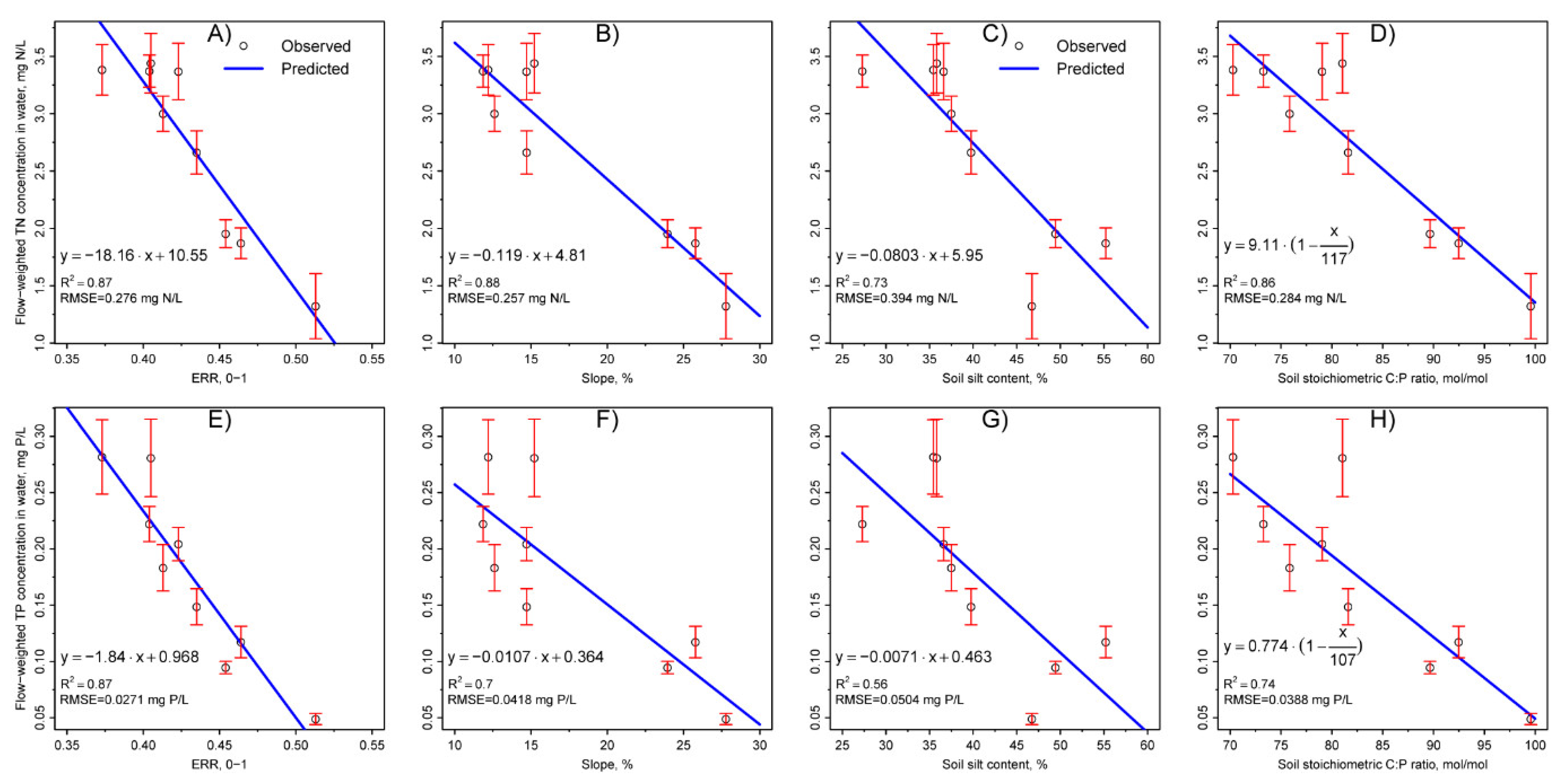
3.2. Topography Played a Hierarchically Important Role in Impacting TN_wc and TP_wc

As shown in Figures S1–S3, the topographical characteristics (e.g., ELEVATION, SLOPE and ERR) had the highest correlations (r = −0.94–−0.93, p < 0.001) with TN_wc, compared to soil properties (r = −0.93–0.72, p = 0.000–0.472) and landscape indicators (r = −0.92–0.91, p = 0.000–0.336). Furthermore, based on Figures S4–S6, two of the topographical characteristics (ELEVATION and ERR) were also found to present the highest correlations (r = −0.93–−0.88, p < 0.002) with TP_wc compared to soil properties (r = −0.86–0.57, p = 0.003–0.734) and landscape indicators (r = −0.85–0.85, p = 0.004–0.142) except for PD (r = 0.92, p < 0.001). Among three topographical characteristics, ELEVATION and SLOPE were highly correlated (r = 0.97, p < 0.001). In addition, ERR presented high correlations with the soil and landscape indicators that were significantly correlated with TN_wc and TP_wc (

Table 6. Pearson’s correlation coefficients between the average elevation–relief ratio and the landscape and soil indicators of the nine studied catchments. *, ** and *** represent the statistical significance at the probability levels of 0.05, 0.01, and 0.001, respectively.

Factor	Indicator	Correlation Coefficient
Landscape (composition)	Woodland	0.91 ***
	Paddy field	−0.93 ***
	Residential area	−0.92 ***
	Pond	−0.92 ***
Landscape (configuration)	LPI	0.93 ***
	ED	−0.89 **
	PD	−0.97 ***
	AI	0.90 ***
	COHESION	0.85 **
	CIRCLE	0.72 *
	SHAPE	0.85 **
	FRAC	0.79 *
	SHDI	−0.90 ***
Landscape (management)	Ninput	−0.87 **
	Pinput	−0.79 *
Soil (Property)	SILT	0.73 *
	SOC	0.75 *
	SOIL_CPR	0.96 ***
	SOIL_NPR	0.89 **

). Thus, topographical characteristics generally had a hierarchical effect on stream water quality at the catchment scale compared with other soil and landscape indicators.

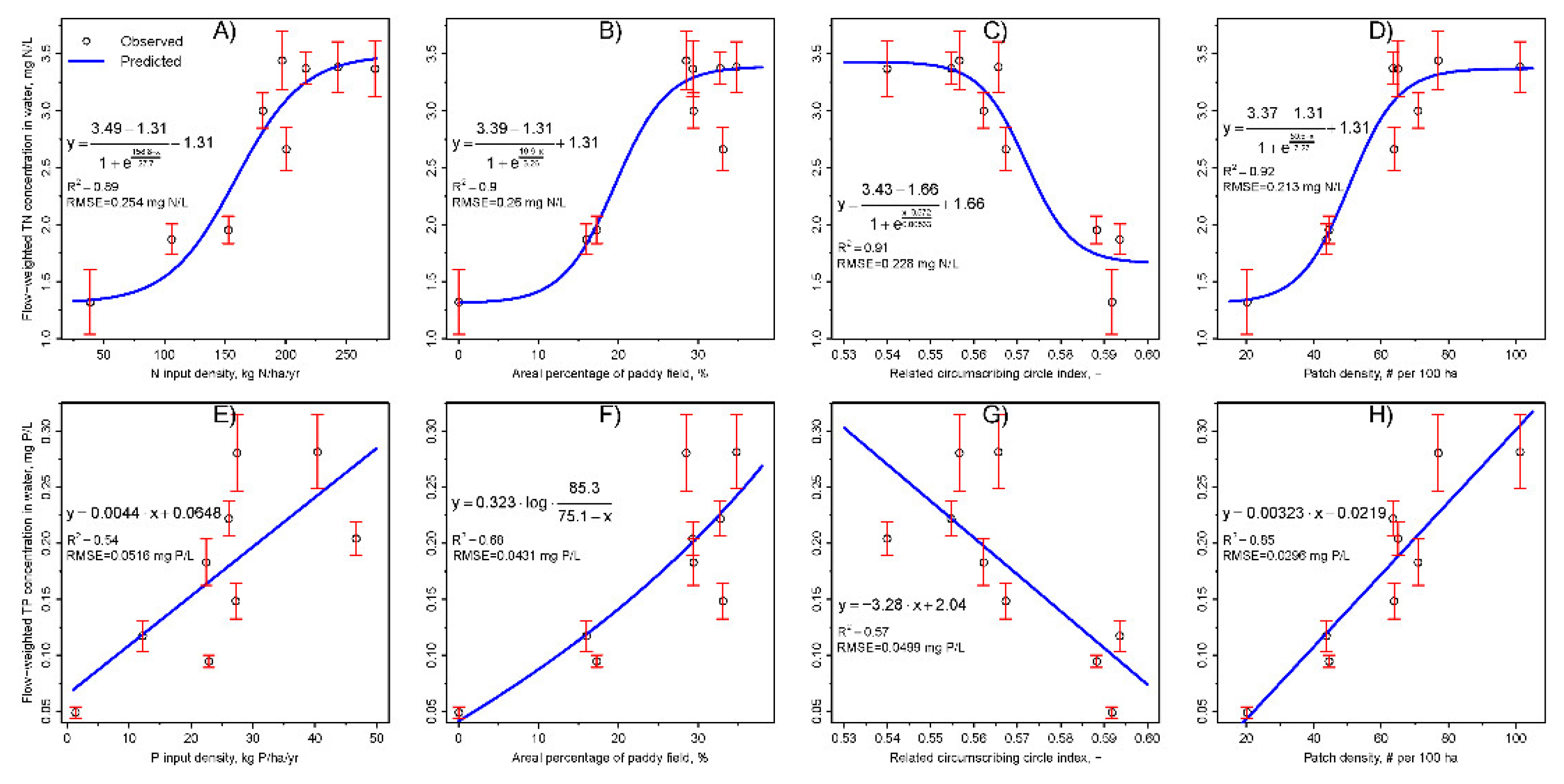
3.3. Paddy Fields Dominated the Impact on TN_wc and TP_wc

The areal percentages of the paddy fields of the nine catchments (Paddy) not only had a significant impact on TN_wc (r = 0.91, p < 0.001) and TP_wc (r = 0.82, p = 0.007) but also showed significant relationships with other landscape indicators, such as Ninput (r = 0.91, p < 0.001), Pinput (r = 0.81, p = 0.008), Woodland (r = −0.99, p < 0.001), Resident (r = 0.98, p < 0.001), Pond (r = 0.88, p = 0.002), LPI (r = −0.99, p < 0.001), PD (r = 0.89, p = 0.001), CIRCLE (r = −0.77, p = 0.016) and SHDI (r = 0.98, p < 0.001) (Figures S1 and S2). This implied that the Paddy indicator dominated the landscape metrics with respect to determining TN_wc and TP_wc in the studied catchments. Thus, Paddy can act as an informative proxy for several other landscape indicators, such as Woodland, Resident, LPI and SHDI.

3.4. Explicit Relationships between TN_wc and TP_wc and the Selected Environmental Factors

Among the topographical, soil and landscape indicators, ERR and SLOPE, representing topography, SILT and SOIL_CPR, representing soil properties; Paddy, representing landscape composition; CIRCLE and PD, representing landscape configuration; and Ninput and Pinput, representing landscape management, were evaluated as the best predictors of the catchment N and P loadings based on the result of the correlation analyses in the previous sections.

As shown in Figure 2A–D, negative linear relationships were well presented for the effects of ERR (y = −18.16·x + 10.55, R² = 0.87, RMSE = 0.276 mg N L⁻¹, p < 0.001), SLOPE (y = −0.119·x + 4.81, R² = 0.89, RMSE = 0.257 mg N L⁻¹, p < 0.001), SILT (y = −0.0803·x + 5.95, R² = 0.73, RMSE = 0.394 mg N L⁻¹, p = 0.003) and SOIL_CPR (y = −0.0779·x + 9.11, R² = 0.86, RMSE = 0.284 mg N L⁻¹, p < 0.001) on TN_wc. In Figure 2(E–H), negative linear relationships were also well presented for the effects of ERR (y = −1.84·x + 0.968, R² = 0.87, RMSE = 0.0271 mg P L⁻¹, p < 0.001), SLOPE (y = −0.0107·x + 0.364, R² = 0.70, RMSE = 0.0418 mg P L⁻¹, p = 0.005), SILT (y = −0.0071·x + 0.463, R² = 0.57, RMSE = 0.0504 mg P L⁻¹, p = 0.020) and SOIL_CPR (y = −0.00723·x + 0.774, R² = 0.74, RMSE = 0.0388 mg P L⁻¹, p = 0.003) on TP_wc; these effects were slightly weaker than those on TN_wc based on the lower R² values. The relationships of TN_wc and TP_wc with SOIL_CPR were reorganized into a linear decreasing equation, as follows:

$$y=y_0·\left(1-\frac{x}{CP{R}_{thr}}\right),$$

(3)

where y₀ is 9.11 mg N L⁻¹ and 0.774 mg P L⁻¹ for TN_wc and TP_wc, respectively, and CPRthr is the threshold of the soil stoichiometric C:P ratio when the N and P loadings to receiving waters approach zero, optimized as 117 and 107 for TN_wc and TP_wc, respectively.

As shown in Figure 3A, TN_wc increased in a nonlinear fashion with increasing N input density in the catchments and leveled off when the Ninput index approached approximately 200 kg N ha⁻¹ yr⁻¹, indicating that further increases in Ninput may not accelerate the deterioration of the stream water quality. This relationship implied that the catchments may have a flat plateau for the TN loading to receiving waters. Such a relationship can be well described by a Boltzmann equation (R² = 0.89, RMSE = 0.254 mg N L⁻¹, p < 0.001):

$$y=\frac{A-B}{1+e^{\frac{C-x}{D}}}+B,$$

(4)

with a maxima of A = 3.49 mg N L⁻¹, a minima of B = 1.31 mg N L⁻¹, a turning point at C = 158.8 kg N ha⁻¹ yr⁻¹ and a slope coefficient of D = 27.7. Both Paddy (Figure 3B) and PD (Figure 3D) presented a similar impact on TN_wc to Ninput, as described by Equation (4), in which more obvious flat plateaus for TN_wc were observed when the areal percentages of the paddy field and landscape patch densities of the catchments were approximately greater than 30% and 75 patches per 100 ha, respectively. The impact of CIRCLE on TN_wc was almost the inverse of that of PD (Figure 3C), except for a slight discrepancy at the end of the curve. As described by McGarigal and Marks [34], the CIRCLE index uses the smallest circumscribing circle to completely cover patches and provides a measure of overall patch elongation. A highly convoluted but narrow patch has a low CIRCLE index due to the relative compactness of the patch, with a high potential of N transport out of the catchments. Conversely, a narrow and elongated patch can have a high linearity index and consequently a high CIRCLE index, with a high potential of N retention in the catchments. The relationship between TN_wc and CIRCLE was fitted to a variant Boltzmann equation (R² = 0.91, RMSE = 0.228 mg N L⁻¹, p < 0.001) with a maxima of 3.43 mg N L⁻¹, a minima of 1.66 mg N L⁻¹ and a turning point at CIRCLE = 0.572.

As shown in Figure 3E,G,H, TP_wc showed linear relationships with Pinput (y = 0.0044·x + 0.0648, R² = 0.54, RMSE = 0.0516 mg P L⁻¹, p = 0.024), CIRLE (y = −3.28·x + 2.04, R² = 0.57, RMSE = 0.0499 mg P L⁻¹, p = 0.019) and PD (y = 0.00323·x−0.0219, R² = 0.85, RMSE = 0.0296 mg P L⁻¹, p < 0.001). In Figure 3F, TP_wc increased exponentially with an increasing Paddy index in the catchments (y = 0.323·log$\frac{85.3}{75.1-x}$, R² = 0.68, RMSE = 0.0431 mg P L⁻¹, p = 0.006). Unlike the relationship of TN_wc with Paddy, there was no observation of a flat plateau for TP_wc when the Paddy index exceeded 30%; in contrast, TP_wc increased at a greater rate. Flat plateaus did not exist in the relationships of TP_wc with Pinput, CIRCLE and PD.

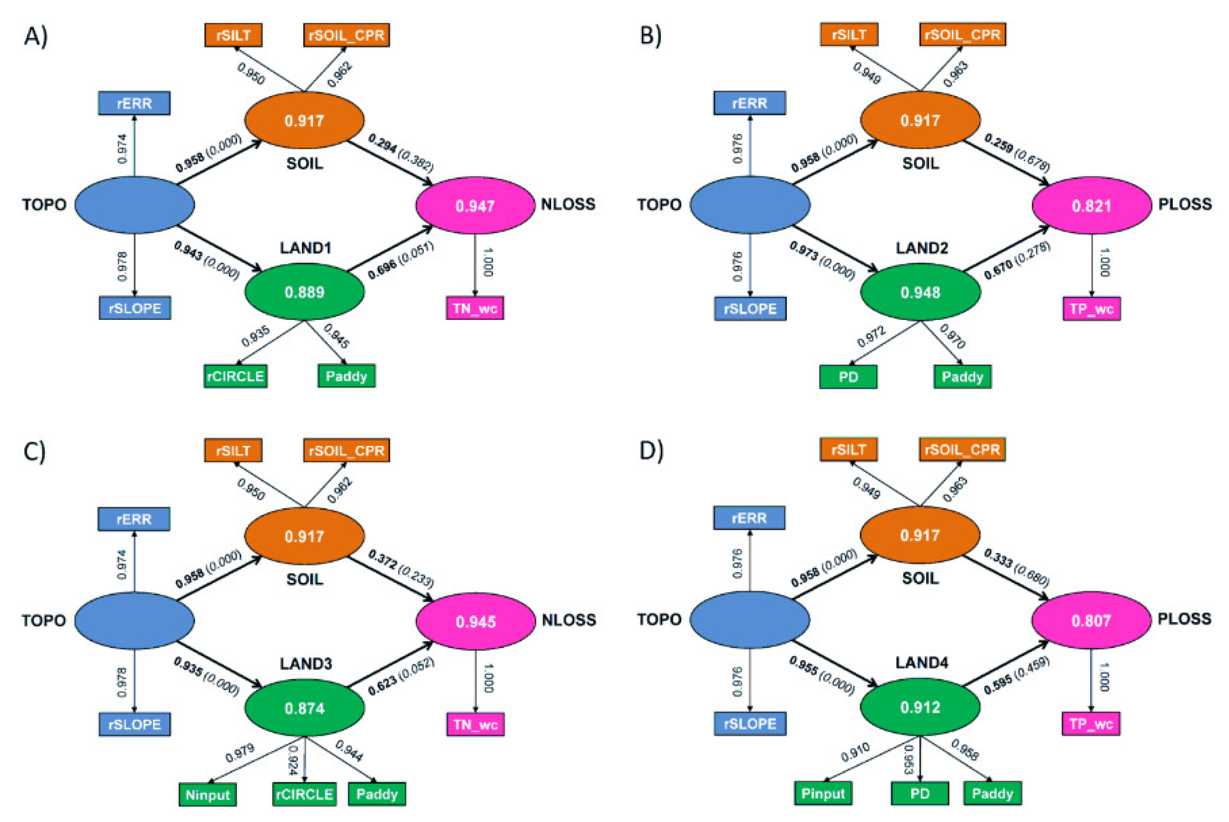
3.5. PLS-SEM Path Analysis

The PLS-SEM path analysis aimed to determine the important pathways of the N and P loadings to receiving waters and included five latent factors: topography (TOPO), soil (SOIL), landscape (LAND), N loading (NLOSS) and P loading (PLOSS). Based on the results of the correlation analyses, TOPO was constructed by two indicators: rERR (1-ERR) and rSLOPE (100-SLOPE); SOIL by two indicators: rSILT (100-SILT) and rSOIL_CPR (117-SOIL_CPR); NLOSS by a single indicator: TN_wc; and PLOSS by a single indicator: TP_wc. The LAND construct had four variants: LAND1 for NLOSS represented by two indicators of Paddy and rCIRCLE (1-CIRCLE); LAND2 for PLOSS by two indicators of Paddy and PD; LAND3 for NLOSS by three indicators of Ninput, Paddy and rCIRCLE (1-CIRCLE); and LAND4 for PLOSS by three indicators of Pinput, Paddy and PD. TOPO was hypothesized to impact NLOSS/PLOSS through two factors: SOIL and LAND.

When landscape management (Ninput and Pinput) was not used to construct the landscape factor, NLOSS and PLOSS were well predicted by TOPO, SOIL and LAND, with R_pls² values of 0.948 and 0.822, respectively (Figure 4A,B and

Table 7. Effects and performance of structural equation models for the path analysis of the relationships of the N and P loadings with the LAND and SOIL factors.

Y	Relationship	Specific Indirect Effect	p Value	Performance
TN_wc	TOPO → SOIL → NLOSS TOPO → LAND1 → NLOSS	0.958 (0.000) × 0.294 (0.382) = 0.282 0.943 (0.000) × 0.696 (0.051) = 0.656	0.389 0.065	Chi-square = 55.96 nfi = 0.596 srmr = 0.063 Rpls2 = 0.947
TP_wc	TOPO → SOIL → PLOSS TOPO → LAND2 → PLOSS	0.958 (0.000) × 0.259 (0.678) = 0.248 0.973 (0.000) × 0.670 (0.278) = 0.563	0.688 0.290	Chi-square = 48.84 nfi = 0.635 srmr = 0.066 Rpls2 = 0.821
TN_wc	TOPO → SOIL → NLOSS TOPO → LAND3 → NLOSS	0.958 (0.000) × 0.372 (0.233) = 0.357 0.935 (0.000) × 0.623 (0.052) = 0.582	0.242 0.073	Chi-square = 88.70 nfi = 0.528 srmr = 0.059 Rpls2 = 0.945
TP_wc	TOPO → SOIL → PLOSS TOPO → LAND4 → PLOSS	0.958 (0.000) × 0.333 (0.680) = 0.318 0.953 (0.000) × 0.595 (0.459) = 0.569	0.689 0.473	Chi-square = 52.00 nfi = 0.638 srmr = 0.071 Rpls2 = 0.807

Note: TOPO was constructed using rERR and rSOLPE; LAND1 was constructed using Paddy and rCIRCLE; LAND2 was constructed using Paddy and PD; LAND3 was constructed using Ninput, Paddy and rCIRCLE; LAND4 was constructed using Pinput, Paddy and PD; SOIL was constructed using rSILT and rSOIL_CPR; rERR= 1–ERR; rSLOPE = 100–SLOPE; rCIRCLE = 1–CIRCLE; rSILT = 100–SILT; rSOIL_CPR = 117–SOIL_CPR. The above variable transformations were essential to achieve a unidimensional variance matrix for SEM analysis. ERR, SLOPE, SILT and SOIL_CPR represent the elevation–relief ratio (dimensionless), the land slope (%), the soil silt content (%) and the soil stoichiometric ratio of carbon to phosphorus (mol mol⁻¹) of the catchments, respectively; while Paddy, PD and CIRCLE represent the areal percentage of the paddy field (%), the patch density (patches per 100 ha) and the related circumscribing index (no dimension, 0–1) of the catchments, respectively. Ninput and Pinput are the catchment N and P input densities (kg N and P ha⁻¹ yr⁻¹), respectively. These variable names are the same hereinafter.

). For TN_wc, the specific indirect effect of the pathway TOPO→LAND1→NLOSS (0.656) was 132% greater than that of TOPO→SOIL→NLOSS (0.282). The TOPO→LAND1→NLOSS pathway was statistically significant at the 0.10 level (p = 0.065), while the TOPO→SOIL→NLOSS pathway was not significant (p = 0.389). This result indicated that the N loading to receiving waters was mostly impacted by topography through the landscape pathway. For TP_wc, the specific indirect effect of the pathway TOPO→LAND2→PLOSS (0.563) was 127% greater than that of TOPO→SOIL→PLOSS (0.248). Neither the TOPO→SOIL→PLOSS pathway nor the TOPO→LAND2→PLOSS pathway was statistically significant at the 0.10 level (p = 0.688 and 0.290, respectively). This implies that the P loading to receiving waters was not dominated by either of these two pathways.

Chi-square is-2 × log (the model likelihood value); nfi is the nonfuzzy index; srmr is the standardized root mean residual; R_pls² is the coefficient of determination for NLOSS and PLOSS predicted by the TOPO, SOIL and LAND factors.

The italicized numbers in the parentheses are the significance probabilities of the path coefficients at the 0.1 level that were determined by 5000 bootstrap replications.

As shown in Figure 4C,D and Table 7, the inclusion of the Ninput and Pinput indicators to construct the landscape factors (LAND3 and LAND4, respectively) did not further improve the predictions of the N and P loadings to receiving waters (R_pls² = 0.945 and 0.807, respectively) compared to Figure 4A,B. In addition, the patterns of pathways impacting the N and P loadings to receiving waters did not change either, even though more N and P management information was used to improve the representativeness of the landscape construct (Table 7).

4. Discussion

4.1. N and P Concentrations in Stream Waters

Compared with the global N and P loadings compiled in the datasets for hundreds of catchments [8,9], the median values of our observed TN_wc (3.00 mg N L⁻¹) and TP_wc (0.183 mg P L⁻¹) (Table S1) are greater than those of global TN_wc (1.23 mg N L⁻¹) by 144% and global TP_wc (0.119 mg P L⁻¹) by 54%, respectively. According to the Environmental Quality Standards for Surface Water of China (GB3838-2002), the stream waters in our nine observed catchments, including a pure woodland catchment, are all polluted by TN (TN > 1.0 mg N L⁻¹) and thus are not drinkable, while four of our nine catchments are contaminated by TP (TP > 0.2 mg P L⁻¹) (see Table 2). TN pollution in stream waters in our region is common and is mostly attributed to a high rate of airborne N deposition, 35–43 kg N ha⁻¹ yr⁻¹ (Dr Jianlin Shen, personal communication, in April 2021) and fertilizer N additions, i.e., 270 kg N ha⁻¹ yr⁻¹ in paddy fields and 450 kg N ha⁻¹ yr⁻¹ in tea fields, where applicable [42].

4.2. Topography

Topographical characteristics (e.g., catchment area, elevation and slope) are important factors that impact stream water quality [5]. As overviewed by [4], catchment elevations or slopes are positively correlated with the TN and TP in stream waters in undeveloped areas (e.g., forests) but are negatively correlated in developed areas (e.g., agriculture and urban areas). Our data agree well with the negative relationships, and we also found a new topographic indicator of ERR was consistently highly correlated with TN_wc and TP_wc (Figure 2). At the landscape scale, topography not only impacts the spatial distribution of soils through the redistributions of energy and materials [30] but also constrains landscape patterns [7]. As presented in Table 6, ERR was significantly correlated with certain soil properties such as SILT (r = 0.73, p = 0.024), SOC (r = 0.75, p < 0.021), SOIL_CPR (r = 0.96, p < 0.001) and SOIL_NPR (r = 0.89, p = 0.001), indicating that topography has a strong impact on soil. ERR proposed by Pike and Wilson [43] is equivalent to the hypsometric integral, which is used to determine the geomorphic stages of development of a catchment and expresses simply how the mass is distributed within a catchment from top to base [44]. On the other hand, paddy fields in our observations were mostly distributed where the topography is relatively flat and the elevation is low, whereas woodlands occur in high elevation regions, also indicating that topography has a strong impact on landscape patterns. As shown in Table 6, ERR was significantly correlated with a number of landscape indicators, such as Paddy (r = −0.93, p < 0.001), Pond (r = −0.92, p < 0.001), PD (r = −0.97, p < 0.001), CIRCLE (r = 0.72, p = 0.029), SHAPE (r = 0.85, p = 0.004), SHDI (r = −0.90, p = 0.001), Ninput (r = −0.87, p = 0.002) and Pinput (r = −0.79, p = 0.011). Therefore, our data and correlation analyses suggested that topography appeared to play a stronger role in determining the N and P loadings to receiving waters than the soil and landscape factors.

4.3. Landscape Composition, Configuration and Management

Landscape composition is closely related to the N and P loadings to receiving waters. Further re-analysis of the global datasets compiled by Alvarez-Cobelas et al. [8,9] indicates that both TN_wc and TP_wc are positively and significantly correlated with the areal percentages of agricultural lands (e.g., cropland and pasture) and are negatively correlated with forests at country scale (e.g., Australia and USA). Our results agree with the above finding, as well as many other reports [18,45,46,47]. The only discrepancy from our study is that we observed a flat plateau for TN_wc when the Paddy index exceeded 30% (Figure 3B), which was not present in the relationship between Paddy and TP_wc (Figure 3F). Based on our previous observations, more than 75% of TN discharged from the catchments are in the soluble forms of NH₄⁺ and NO₃⁻, while more than 50% of TP is in the form of particulate P attached to soil sediments transported in runoff [15]. Because the soluble forms of TN in catchment surface water are subject to pathways for loss such as mineralization, nitrification, denitrification, and biological assimilations by microbes, algae, and aquatic plants [48], a flat plateau for Paddy versus TN_wc in our catchments (Figure 3B) is understandable. Such a phenomenon may also imply that a paddy field or an artificial wetland ecosystem has two kinds of abilities in relation to the TN fate in the catchment: discharge and retention. A certain extent of aggregation of the paddy field may significantly favor TN retention in catchments via the paddy field itself and the surrounding drainage ditches on the route to stream waters, in agreement with [49]. TP_wc is mostly generated by soil water erosion (e.g., [12,50]). Even though the soluble form of TP can be captured by biological assimilations and can be adsorbed by soil sediments, the proportion of re-settled TP in catchments is very limited, resulting in an exponentially increasing relationship between Paddy and TP_wc.

The landscape configuration metrics are more informative than the landscape composition metrics and the N and P input densities to account for the N and P loadings of catchments [19]. Recently, a few attempts have been made to explore the relationships between water quality and catchment landscape configuration at the class and landscape levels from a landscape ecology perspective, e.g., [2,11,14,15,18,51,52,53,54,55]. However, most of those previous investigations focused only on the impact of landscape configuration metrics on water quality in adjacent aquatic systems, rather than the N and P loadings directly discharged from catchments. Nevertheless, those studies found PD, LPI, ED, AI, and SHDI in variable relationships with the TN and TP concentrations in adjacent rivers, ponds, lakes, and reservoirs at both the class and landscape levels. In our studied catchments, TN_wc was negatively correlated with LPI (r = −0.92, p < 0.001), SHAPE (r = −0.86, p = 0.003), CIRCLE (r = −0.91, p < 0.001), and AI (r = −0.77, p = 0.016) and positively correlated with ED (r = 0.76, p = 0.016), PD (r = 0.88, p = 0.002) and SHDI (r = 0.89, p = 0.001) at the landscape level (Figure S2). Liu et al. [18] argued that the landscape configuration indices at the class level are more strongly correlated with water quality than at the landscape level. However, in our case, these metrics at the landscape level were sufficiently informative. TN_wc was best predicted by PD with the Boltzmann equation (Equation (4)) shown in Figure 3D (R² = 0.92, RMSE = 0.213 mg N L⁻¹, p < 0.001). As PD is a measure of the landscape fragmentation process in the region [34], Figure 3D indicates that the fragmentation process gradually increased the catchment N loading in the early stages (PD = 10–40 patches per 100 ha), with a more dramatic increase in the middle stage (PD = 40–60 patches per 100 ha); when PD exceeded 70 patches per 100 ha, the increase in TN_wc as a result of the PD increase was limited. In other words, regardless of how the landscape was fragmented, TN_wc had a flat plateau, at least in our observed catchments (3.37 mg N L⁻¹). For catchment water quality management, to maintain stream water quality within the GB3838-2002 framework in terms of TN on an annual basis (TN_wc ≤ 2 mg N L⁻¹), the PD of a given catchment in our region must be lower than 45 patches per 100 ha. Of course, such a PD threshold is influenced by regional atmospheric N deposition. The lower the atmospheric N deposition, the lower the PD threshold.

In our nine studied catchments, TP_wc was negatively correlated with LPI (r = −0.84, p = 0.005), SHAPE (r = −0.72, p < 0.028), CIRCLE (r = −0.75, p = 0.019), COHESION (r = −0.85, p = 0.004), and AI (r = −0.76, p = 0.016) and was positively correlated with ED (r = 0.76, p = 0.018), PD (r = 0.92, p < 0.001) and SHDI (r = 0.78, p = 0.013) (Figure S5). As a result, TP_wc was again found to be best predicted by PD using the linear regression model shown in Figure 3H (R² = 0.85, RMSE = 0.0296 mg P L⁻¹, p < 0.001). To ensure stream water quality within the drinkable level in terms of TP (TP ≤ 0.2 mg P L⁻¹), we may need to slow down the landscape fragmentation process such that PD < 70 patches per 100 ha. Therefore, combined with the relationship between PD and TN_wc, the stream water quality (TN_wc and TP_wc) of catchments can be managed by tuning the very informative landscape structure index, i.e., PD, in a catchment development plan. Due to the complexity of landscape evolution at the catchment scale, the universal application of the PD index in this study to other regions, countries, or continents is unnecessary. For catchment systems with a large backdrop mosaic (such as a forest or grassland) invaded by anthropogenic activity-dominated land use types (such as croplands), the PD may work. Otherwise, the following landscape configuration metrics may apply: ED, SHAPE, CIRCLE and SHDI, depending on their own suitability.

Theoretically, the landscape management indicators (Ninput and Pinput) were more informative in relation to the N and P loadings than the landscape composition indicators such as Paddy, as they consider not only the areal percentages of landscape compositions, but also the N and P inputs in individual landscape compositions in the catchments. A number of researchers have stated that the N and P input sources are strongly related to N and P loadings, e.g., [8,9,56,57]. However, the quantitative relationships of Ninput and Pinput with TN_wc and TP_wc in this study were not stronger than those of the landscape indices for composition and configuration (Figure 3A,E versus Figure 3B–D,F–H), indicating that the N and P source factors (Ninput and Pinput) are important for but not deterministic of the N and P loadings of catchments to receiving waters.

4.4. Soil Properties

Soil is an important medium, acting as a source, sink and transport platform for N and P nutrients from catchments to receiving waters. However, the soil properties of catchments, including elemental stoichiometric ratios, were rarely related to the N and P loadings in previous investigations, except in relation to the soil sorption capacity [58] and soil drainage capacity [22,59]. Varanka et al. [58] observed positive correlations between TN and TP concentrations in rivers and the silt and clay contents of catchment soils in Finland and thus argued that higher silt and clay contents in soils result in greater soil adsorption of N and P nutrients. Higher N and P concentrations were observed in the streams of catchments where soils are mostly well drained in the United States [22] and Sweden [59]. In this study, we found that TN_wc was not correlated with TSN (r = −0.33, p = 0.388) but was negatively correlated with SILT (r = −0.85, p = 0.003), SOC (r = −0.80, p = 0.010), SOIL_CPR (r = −0.93, p < 0.001) and SOIL_NPR (r = −0.91, p < 0.001) (Figure S3). As a result, the SOIL_CPR indicators were identified as the best predictors for N loading to receiving waters (see the relationships in Figure 2D). TP_wc was not significantly correlated with TSP (r = 0.36, p = 0.345) but was negatively correlated with SILT (r = −0.75, p = 0.020), SOC (r = −0.71, p = 0.033), SOIL_CPR (r = −0.86, p = 0.003) and SOIL_NPR (r = −0.84, p = 0.005) (Figure S6). Again, the SOIL_CPR indicator was found to be the best predictor for the P loading to receiving waters (see Figure 2H). Interestingly, TN_wc and TP_wc responded to individual important soil properties of catchments in a similar way, including the same signs of correlations, despite slight discrepancies in the strengths of correlations. Such a consistent relationship can be explained by the fact that the increasing elemental P input (e.g., resulting from the intrusion of the paddy fields into land formerly occupied by Masson pine woodland) into the catchment causes a decrease in the soil C:P ratio and might improve the mobility of soil N (e.g., NH₄⁺, NO₃⁻ and dissolved organic N) as well as reactive P in the catchment [60,61].

The relationships of TN_wc and TP_wc with SOIL_CPR illustrated in Figure 2D,H and described using Equation (1) suggested that decreasing the application rate of fertilizer P in our catchments, if applicable, could help to reduce both N and P discharges from catchments to receiving stream waters. The parameter CPR_thr in Equation (3) can also serve as a soil element threshold ratio (ETR) at which the catchment N or P loadings approach zero. In our case, it is in the range of 107 to 117. Sterner and Elser [62] stated that the stoichiometric ratios of C, N and P of ecosystems reflect the severity of autotroph nutrient limitation and the degree to which heterotrophs are energy versus nutrient limited. These stoichiometric ratios can influence ecosystem services (e.g., water quality and eutrophication) [63,64,65]. As N and P nutrients travel through catchments, they may be transported downstream, sequestered or lost to the atmosphere at different rates and efficiencies as a result of the stoichiometric ratios of C, N and P of ecosystems. Liu et al. [63] found that the high C: P and N: P ratios in phototrophic biofilms favored phosphorus immobilization in biofilm biomass, increasing the abundance of green algae in Chinese paddy fields. From the element biogeochemical cycle perspective, the influence of stoichiometric ratios of C, N and P on N and P pathways in the catchment is not well defined. For example, in our case, SOIL_CPR was calculated by SOC divided by TSP. SOC occurs completely in organic form and is composed of soil microbial biomass C and humus C, while TSP consists of soil organic P (soil microbial biomass P and humus P, accounting for approximately 40% of TSP) and inorganic P (soil labile P and deposited mineral P). Li et al. [66] reported a significant correlation between the soil and soil microbial biomass C:P ratios (r = 0.56, p < 0.001, n = 1069) in three landscapes of subtropical China. As the decomposable organic matter C:P ratios are negatively correlated with their decomposition rate constants, e.g., [67,68], our data may imply that the catchment nutrient loadings are related to soil organic matter decomposition, which agrees with Manzoni and Porporato [69]. Our speculation for such a strong negative relationship is that in a P-limiting environment (e.g., red soil region in southern China) the soil microbial C:P ratio, which is significantly correlated with soil C:P ratio [66], is a key factor to determine the N and P turnover in soils, consequently impact the N and P availability [70,71], and eventually enhance the N and P plant uptake and surface runoff transport. The balance between the last two is highly dependent on the frequency of rainfall and surface runoff events, which is fairly high in the studied areas. Which components of soil C and P of catchments play a key role in regulating the relationships in Figure 2D,H, and how? The answer to such questions will provide more detailed insights into the N and P nutrient cycles through catchments, and thus, further research is needed.

4.5. Catchment N and P Path Analyses

The PLS-SEM path analysis indicated that the specific indirect effect of the TOPO→LAND1/3→NLOSS pathway (p = 0.051–0.052) was significantly greater than that of the TOPO→SOIL→NLOSS pathway (p = 0.233–0.382) (Table 7 and Figure 4A,C), suggesting that emphatic strategies to control catchment N loss to receiving waters need to focus on catchment landscape ecosystems rather than on soils on which mitigation practices are normally based. In landscape ecosystems, we should not only look at the areas of paddy fields (including N inputs) and the shapes of landscape patches but should also pay more attention to aquatic ecosystems (e.g., drainage ditches and headwater stream reaches) due to the residence time issue related to N transport through these linear structures in catchments [48,72]. Streams and rivers in catchments represent key ecosystems for nutrient storage, transformations and removal (a set of processes for nutrient retention) [73,74]. In-stream nutrient retention is a result of the interaction between hydrological and biogeochemical processes involved in downstream transport. Marcé et al. [75] compiled a dataset of 82 published studies and found that the biogeochemical reactivity (e.g., assimilatory/dissimilatory uptake and adsorption/co-precipitation) explained 62% of the variability in nutrient (particularly ammonium) retention in streams, while other catchment hydrological factors such as discharge, channel morphology and water transient storage also impact stream nutrient retention due to the responsive contact time between nutrients and reactive mediums in the water column [48].

With respect to catchment P loss, although the specific indirect effect of the TOPO→LAND2/4→PLOSS pathway (p = 0.278–0.459) was greater than the specific indirect effect of the TOPO→SOIL→PLOSS pathway (p = 0.678–0.680), none of these pathways were statistically significant (p > 0.10) (Table 7 and Figure 4B,D), informing us that the strategies to control catchment P loss to receiving waters need to be applied to both soils and landscape ecosystems without pathway preference. While the N control practices through aquatic systems may also capture runoff P loss simultaneously, to reduce the catchment P loading to receiving waters, the P control practices can be cost-effectively focused on the soil medium, such as controlling the soil water erosion rate [76,77]. At the landscape level, streams and wetlands form a critical interface between uplands/soils and adjacent water bodies for P transport and retention, as these ecosystems are hydrologically linked [78,79]. When evaluating P retention in streams and wetlands, it is suggested that both biotic (e.g., assimilation by vegetation, plankton, periphyton, and microorganisms) and abiotic (e.g., sedimentation, adsorption by sediments/soils, precipitation, and exchange between soil/sediment and the overlying water column) processes need to be taken into account. A comprehensive review by Reddy et al. [79] concluded that P retention in streams and wetlands is dominated by physical processes such as flow velocity, discharge, and water depth. However, long-term storage of P in stream sediments can be spiraled by rapid mobilization and transport that occurs during large runoff events.

In addition, to simplify the process of evaluating the catchment N and P loadings, a costly field survey to obtain the detailed catchment N and P input densities could be avoided, as the PLS-SEM path analyses with Ninput and Pinput as indicators for LAND (Table 7 and Figure 4A,B) did not outperform the analyses without Ninput and Pinput (Table 7 and Figure 4C,D). This finding also indicated that the landscape metrics for composition (Paddy) and configuration (CIRCLE and PD) were sufficiently informative to construct the LAND factor for the PLS-SEM analyses carried out in this study. Lintern et al. [4] overviewed a number of statistical methods (e.g., multiple regression, geographic weighted regression, variance partitioning, boosted regression tree, artificial neural network, fuzzy rule-based model and self-organizing map) to investigate the relationships between landscape characteristics and water quality. In addition, Varanka and Luoto [80] found that the areal percentage of agricultural lands in the catchment was the most important factor affecting TP and TN concentrations in Finland by applying variation and hierarchical partitioning methods. However, these previous studies were less concerned about how to identify the dominant pathways for N and P loss at the catchment scale.

5. Conclusions

At the catchment scale in the subtropics, N and P runoff losses were impacted by topography, soil and landscape, and topography played a hierarchical role. Our findings on the explicit relationships between the N loading to receiving waters and catchment elevation, the soil elemental stoichiometric ratio and landscape metrics suggested that to reduce N export from agricultural catchments, not only should the traditional strategies for soils be implemented, but prevention practices in landscape ecosystems, such as planning the proportions of paddy fields (e.g., areas and N inputs) and the shapes of landscape patches, as well as managing the aquatic systems (e.g., ditches and streams) to tackle the N transport/residence time, should also be emphatically deployed. Strategies to lower catchment P export from soils may simply be proposed at the site. Conceptually, decreasing the P fertilizer application in catchments (if applicable) to increase the catchment soil C:P ratio can effectively reduce both the N and P loadings of catchments receiving stream waters. To deepen our understanding of the transport and retention of N and P nutrients in catchments in the subtropics, the following two areas are in need of further investigation: the N retention mechanism of the aggregated paddy fields and the differentiation of the impact of the soil stoichiometric C:P ratio on the catchment N and P loadings.

References

1. Bussi, G.; Janes, V.; Whitehead, P.G.; Dadson, S.J.; Holman, I.P. Dynamic response of land use and river nutrient concentration to long-term climatic changes. Sci. Total Environ. 2017, 590–591, 818–831. [Google Scholar] [CrossRef] [PubMed]
2. Ding, J.; Jiang, Y.; Liu, Q.; Hou, Z.; Liao, J.; Fu, L.; Peng, Q. Influences of the land use pattern on water quality in low-order streams of the Dongjiang River basin, China: A multi-scale analysis. Sci. Total Environ. 2016, 551–552, 205–216. [Google Scholar] [CrossRef] [PubMed]
3. Forman, R.T.T. Land Mosaics: The Ecology of Landscapes and Regions; Cambridge University Press: London, UK, 1995. [Google Scholar]
4. Lintern, A.; Webb, J.A.; Ryu, D.; Liu, S.; Bende-Michl, U.; Waters, D.; Leahy, P.; Wilson, P.; Western, A. Key factors influencing differences in stream water quality across space. Wiley Interdiscip. Rev. Water 2017, 5, e1260. [Google Scholar] [CrossRef] [Green Version]
5. Arnold, J.G.; Srinivasan, R.; Muttiah, R.S.; Williams, J.R. Large area hydrologic modeling and assessment Part I: Model development. J. Am. Water Resour. Assoc. 1998, 34, 73–89. [Google Scholar] [CrossRef]
6. Lintern, A.; Webb, J.A.; Ryu, D.; Liu, S.; Waters, D.; Leahy, P.; Bende-Michl, U.; Western, A.W. What are the key catchment characteristics affecting spatial differences in riverine water quality? Water Resour. Res. 2018, 54, 7252–7272. [Google Scholar] [CrossRef]
7. Ye, L.; Cai, Q.; Liu, R.; Cao, M. The influence of topography and land use on water quality of Xiangxi River in Three Gorges Reservoir region. Environ. Geol. 2009, 58, 937–942. [Google Scholar] [CrossRef]
8. Alvarez-Cobelas, M.; Angeler, D.G.; Sanchez-Carrillo, S. Export of nitrogen from catchments: A worldwide analysis. Environ. Pollut. 2008, 156, 261–269. [Google Scholar] [CrossRef]
9. Alvarez-Cobelas, M.; Sanchez-Carrillo, S.; Angeler, D.G.; Sanchez-Andres, R. Phosphorus export from catchments: A global view. J. North Am. Benthol. Soc. 2009, 28, 805–820. [Google Scholar] [CrossRef] [Green Version]
10. Kearns, F.R.; Kelly, N.M.; Carter, J.L.; Resh, V.H. A method for the use of landscape metrics in freshwater research and management. Landsc. Ecol. 2005, 20, 113–125. [Google Scholar] [CrossRef]
11. Lee, S.W.; Hwang, S.J.; Lee, S.B.; Hwang, H.S.; Sung, H.C. Landscape ecological approach to the relationships of land use patterns in watersheds to water quality characteristics. Landsc. Urban Plan. 2009, 92, 80–89. [Google Scholar] [CrossRef]
12. Shen, Z.Y.; Chen, L.; Hong, Q.; Qiu, J.L.; Xie, H.; Liu, R.M. Assessment of nitrogen and phosphorus loads and causal factors from different land use and soil types in the Three Gorges Reservoir Area. Sci. Total Environ. 2013, 454–455, 383–392. [Google Scholar] [CrossRef] [PubMed]
13. Turner, M.G.; Gardner, R.H.; O’Neill, R.V. Landscape Ecology in Theory and Practice. Geography 2003, 83, 479–494. [Google Scholar]
14. Uuemaa, E.; Roosaare, J.; Mander, Ü. Landscape metrics as indicators of river water quality at catchment scale. Nord. Hydrol. 2007, 38, 125–138. [Google Scholar] [CrossRef]
15. Wang, Y.; Li, Y.; Liu, X.L.; Liu, F.; Li, Y.Y.; Song, L.F.; Li, H.; Ma, Q.M.; Wu, J. Relating land use patterns to stream nutrient levels in red soil agricultural catchments in subtropical central China. Environ. Sci. Pollut. Res. 2014, 21, 10481–10492. [Google Scholar] [CrossRef] [PubMed]
16. Wickham, J.D.; Wade, T.G.; Ritters, K.H.; O’Neill, R.V.; Smith, J.H.; Smith, E.R.; Jones, K.B.; Neale, A.C. Upstream-to-downstream changes in nutrient export risk. Landsc. Ecol. 2003, 18, 193–206. [Google Scholar] [CrossRef]
17. Alexander, R.B.; Smith, R.A.; Schwarz, G.E. Effect of stream channel size on the delivery of nitrogen to the Gulf of Mexico. Nature 2000, 403, 758. [Google Scholar] [CrossRef] [PubMed]
18. Liu, W.; Zhang, Q.; Liu, G. Influences of watershed landscape composition and configuration on lake-water quality in the Yangtze River basin of China. Hydrol. Process. 2012, 26, 570–578. [Google Scholar] [CrossRef]
19. Billmire, M.; Koziol, B.W. Landscape and flow path-based nutrient loading metrics for evaluation of in-stream water quality in Saginaw Bay, Michigan. J. Great Lakes Res. 2018, 44, 1068–1080. [Google Scholar] [CrossRef]
20. Drewry, J.J.; Newham, L.T.H.; Greene, R.S.B.; Jakeman, A.J.; Croke, B.F.W. A review of nitrogen and phosphorus export to waterways: Context for catchment modeling. Mar. Freshw. Res. 2006, 57, 757–774. [Google Scholar] [CrossRef]
21. Kleinman, P.J.A.; Sharpley, A.N.; McDowell, R.W.; Flaten, D.N.; Buda, A.R.; Tao, L.; Bergstrom, L.; Zhu, Q. Managing agricultural phosphorus for water quality protection: Principles for progress. Plant Soil 2011, 349, 169–182. [Google Scholar] [CrossRef]
22. Franklin, D.H.; Steiner, J.L.; Duke, S.E.; Moriasi, D.N.; Starks, P.J. Spatial considerations in wet and dry periods for phosphorus in streams of the Fort Cobb Watershed, United States. J. Am. Water Resour. Assoc. 2013, 49, 908–922. [Google Scholar] [CrossRef]
23. Fan, Y.; Chen, J.; Shirkey, G.; John, R.; Wu, S.R.; Park, H.; Shao, C.L. Applications of structural equation modeling (SEM) in ecological studies: An updated review. Ecol. Process. 2016, 5, 19. [Google Scholar] [CrossRef] [Green Version]
24. Hoyle, R.H. Structural Equation Modeling: Concepts, Issues, and Applications; SAGE Publications: Thousand Oaks, CA, USA, 1995. [Google Scholar]
25. Wold, H. Estimation of principal component and related models by iterative least squares. In Multivariate Analysis; Krishnaiah, P., Ed.; Academic Press: New York, NY, USA, 1966; pp. 391–420. [Google Scholar]
26. Lohmoeller, J.B. Latent Variable Path Modeling with Partial Least Squares; Physica: Heidelberg, Germany, 1989. [Google Scholar]
27. Hair, J.F.; Hult GT, M.; Ringle, C.M.; Sarstedt, M. A Primer on Partial Least Squares Structural Equation Modeling (PLS-SEM), 2nd ed.; SAGE Publications: Thousand Oaks, CA, USA, 2017. [Google Scholar]
28. Cooperative Research Group on Chinese Soil Taxonomy. Chinese Soil Taxonomy; Sciences Press: Beijing, China; New York, NY, USA, 2001. [Google Scholar]
29. Mitchell, A. The ESRI Guide to GIS Analysis; ESRI Press: Redlands, CA, USA, 2008; Volume 2. [Google Scholar]
30. Jenny, H. Factors of Soil Formation: A System of Quantitative Pedology; McGraw-Hill: New York, NY, USA, 1941. [Google Scholar]
31. Li, W.; Xu, X.P. Hydraulics; The Press of Wu Han Hydraulic and Power University: Wuhan, China, 1999. (In Chinese) [Google Scholar]
32. Tang, J.L.; Zhang, B.; Gao, C.; Zepp, H. Hydrological pathway and source area of nutrient losses identified by a multi-scale monitoring in an agricultural catchment. Catena 2008, 72, 374–385. [Google Scholar] [CrossRef]
33. Water Resources Research Laboratory, USA. Water Measurement Manual. 2001. Available online: http://www.usbr.gov/pmts/hydraulicslab/pubs/wmm (accessed on 1 January 2012).
34. McGarigal, K.; Marks, B.J. FRAGSTATS: Spatial Pattern Analysis Program for Quantifying Landscape Structure; General Technical Report PNW-GTR-351; U.S. Department of Agriculture, Forest Service, Pacific Northwest Research Station: Portland, OR, USA, 1995. [Google Scholar]
35. McGarigal, K.; Cushman, S.A.; Ene, E. FRAGSTATS v4: Spatial Pattern Analysis Program for Categorical and Continuous Maps. Computer Software Program Produced by the Authors at the University of Massachusetts, Amherst, 2012. Available online: http://www.umass.edu/landeco/research/fragstats/fragstats.html (accessed on 1 December 2016).
36. Shao, X.Q. Temporal and Spatial Variation in Atmospheric Nitrogen and Phosphorus Deposition in Four Forest Types in Different Climatic Regions. Master’s Thesis, Northwest A&F University, Xianyang, China, 2018; p. 47. [Google Scholar]
37. Han, Y.G.; Yu, X.X.; Wang, X.X.; Wang, Y.Q.; Tian, J.X.; Xu, L.; Wang, C.Z. Net anthropogenic phosphorus inputs (NAPI) index application in Mainland China. Chemosphere 2013, 90, 329–337. [Google Scholar] [CrossRef] [PubMed]
38. Han, Y.G.; Fan, Y.T.; Yang, P.L.; Wang, X.X.; Wang, Y.J.; Tian, J.X.; Xu, L.; Wang, C.Z. Net anthropogenic nitrogen inputs (NANI) index application in Mainland China. Geoderma 2014, 213, 87–94. [Google Scholar] [CrossRef]
39. R Core Team. R: A Language and Environment for Statistical Computing; R Foundation for Statistical Computing; R Core Team: Vienna, Austria, 2018; Available online: https://www.R-project.org (accessed on 1 December 2018).
40. Garson, G.D. Partial Least Squares: Regression and Structural Equation Models; Statistical Associates Publishers: Asheboro, NC, USA, 2016. [Google Scholar]
41. Ringle, C.M.; Wende, S.; Becker, J.-M. SmartPLS 3; SmartPLS GmbH: Boenningstedt, Germany, 2015; Available online: https://www.smartpls.com (accessed on 1 January 2018).
42. Shen, J.L.; Li, Y.; Liu, X.J.; Luo, X.S.; Tang, H.; Zhang, Y.Z.; Wu, J. Atmospheric dry and wet nitrogen deposition on three contrasting land use types of an agricultural catchment in subtropical central China. Atmos. Environ. 2013, 67, 415–424. [Google Scholar] [CrossRef]
43. Pike, R.J.; Wilson, S.E. Elevation-relief ratio, hypsometric integral and geomorphic area-altitude analysis. Geol. Soc. Am. Bull. 1971, 62, 1079–1084. [Google Scholar] [CrossRef]
44. Langbein, W.B. Topographic Characteristics of Drainage Basins; US Geological Survey Water-Supply Paper; U.S. Government Publishing Office: Washington, DC, USA, 1947; Volume 986, pp. 157–159. [Google Scholar]
45. Lenat, D.R.; Crawford, J.K. Effects of land use on water quality and aquatic biota of three North Carolina Piedmont streams. Hydrobiologia 1994, 294, 185–199. [Google Scholar] [CrossRef]
46. Li, S.; Gu, S.; Liu, W.; Han, H.; Zhang, Q. Water quality in relation to land use and land cover in the upper Han River Basin, China. Catena 2008, 75, 216–222. [Google Scholar] [CrossRef]
47. Tong, S.T.; Chen, W. Modeling the relationship between land use and surface water quality. J. Environ. Manag. 2002, 66, 377–393. [Google Scholar] [CrossRef]
48. Peterson, B.J.; Wollheim, W.M.; Mulholland, P.J.; Webster, J.R.; Meyer, J.L.; Tank, J.L.; Marti, E.; Bowden, W.B.; Valett, H.M.; Hershey, A.E.; et al. Control of nitrogen export from watersheds by headwater streams. Science 2001, 292, 86–92. [Google Scholar] [CrossRef]
49. Li, S.; Liu, H.; Zhang, L.; Li, X.; Wang, H.; Zhuang, Y.; Zhang, F.; Zhai, L.; Fan, X.; Hu, W.; et al. Potential nutrient removal function of naturally existed ditches and ponds in paddy regions: Prospect of enhancing water quality by irrigation and drainage management. Sci. Total Environ. 2020, 718, 137418. [Google Scholar] [CrossRef] [PubMed]
50. Janeau, J.L.; Gillard, L.C.; Grellier, S.; Jouquet, P.; Thi Phuong Quynhf, L.; Thi Nguyet Minh, L.; Quoc Anh, N.; Orange, D.; Dinh Rinh, P.; Duc Toan, T.; et al. Soil erosion, dissolved organic carbon and nutrient losses under different land use systems in a small catchment in northern Vietnam. Agric. Water Manag. 2014, 146, 314–323. [Google Scholar] [CrossRef]
51. Amiri, B.J.; Nakane, K. Modeling the linkage between river water quality and landscape metrics in the Chugoku District of Japan. Water Resour. Manag. 2009, 23, 931–956. [Google Scholar] [CrossRef]
52. Johnson, L.; Richards, C.; Host, G.; Arthur, J. Landscape influences on water chemistry in Midwestern stream ecosystems. Plant J. 1997, 37, 193–208. [Google Scholar] [CrossRef]
53. Moreno-Mateos, D.; Mander, U.; Comin, F.A.; Pedrocchi, C.; Uuemaa, E. Relationships between landscape pattern, wetland characteristics, and water quality in agricultural catchments. J. Environ. Qual. 2008, 37, 2170–2180. [Google Scholar] [CrossRef] [PubMed]
54. Uuemaa, E.; Roosaare, J.; Mander, Ü. Scale dependence of landscape metrics and their indicatory value for nutrient and organic matter losses from catchments. Ecol. Indic. 2005, 5, 350–369. [Google Scholar] [CrossRef]
55. Xiao, H.; Ji, W. Relating landscape characteristics to non-point source pollution in mine waste-located watersheds using geospatial technique. J. Environ. Manag. 2007, 82, 111–119. [Google Scholar] [CrossRef]
56. Gao, C.; Zhu, J.G.; Zhu, J.Y.; Gao, X.; Dou, Y.J.; Hosen, Y. Nitrogen export from an agriculture watershed in the Taihu Lake area, China. Environ. Geochem. Health 2004, 26, 199–207. [Google Scholar] [CrossRef]
57. Howarth, R.W. An assessment of human influences on fluxes of nitrogen from the terrestrial landscape to the estuaries and continental shelves of the North Atlantic Ocean. Nutr. Cycl. Agroecosystems 1998, 52, 213–223. [Google Scholar] [CrossRef]
58. Varanka, S.; Hjort, J.; Luoto, M. Geomorphological factors predict water quality in boreal river. Earth Surf. Process. Landf. 2015, 40, 1989–1999. [Google Scholar] [CrossRef]
59. Arheimer, B.; Lidden, R. Nitrogen and phosphorus concentrations from agricultural catchments—Influence of spatial and temporal variables. J. Hydrol. 2000, 227, 140–159. [Google Scholar] [CrossRef]
60. Penuelas, J.; Poulter, B.; Sardans, J.; Ciais, P.; Van Der Velde, M.; Bopp, L.; Boucher, O.; Godderis, Y.; Hinsinger, P.; Llusia, J.; et al. Human-induced nitrogen-phosphorus imbalances alter natural and managed ecosystems across the globe. Nat. Commun. 2013, 4, 2934. [Google Scholar] [CrossRef] [PubMed] [Green Version]
61. Toth, J.D.; Dou, Z.; Ferguson, J.D.; Galligan, D.T.; Ramberg, C.F., Jr. Nitrogen- vs. phosphorus-based dairy manure applications to field crops: Nitrate and phosphorus leaching and soil phosphorus accumulation. J. Environ. Qual. 2006, 35, 2302–2312. [Google Scholar] [CrossRef] [PubMed]
62. Sterner, R.W.; Elser, J.J. Ecological Stoichiometry: The Biology of Elements from Molecules to the Biosphere; Princeton University Press: Princeton, NJ, USA, 2002. [Google Scholar]
63. Liu, J.Z.; Sun, P.F.; Sun, R.; Wang, S.C.; Gao, B.; Tang, J.; Wu, Y.H.; Dolfing, J. Carbon-nutrient stoichiometry drives phosphorus immobilization in phototrophic biofilms at the soil-water interface in paddy fields. Water Res. 2019, 167, 115129. [Google Scholar] [CrossRef]
64. Schindler, D.W.; Hecky, R.E.; Findlay, D.L.; Station, M.P.; Parker, B.R.; Paterson, M.J.; Beaty, K.G.; Lyng, M.; Kasian, S.E.M. Eutrophication of lakes cannot be controlled by reducing nitrogen input: Results of a 37-year whole-ecosystem experiment. Proc. Natl. Acad. Sci. USA 2008, 105, 11254–11258. [Google Scholar] [CrossRef] [Green Version]
65. Smith, V.H. Low nitrogen to phosphorus ratios favor dominance by blue-green algae in lake phytoplankton. Science 1983, 221, 669–671. [Google Scholar] [CrossRef] [Green Version]
66. Li, Y.; Wu, J.; Liu, S.; Shen, J.L.; Huang, D.; Su, Y.R.; Wei, W.X.; Syers, J.K. Is the C:N:P stoichiometry in soil and soil microbial biomass related to the landscape and land use in southern subtropical China? Glob. Biogeochem. Cycles 2012, 26, 1–14. [Google Scholar] [CrossRef]
67. Zechemeister-Boltenstern, S.; Keiblinger, K.M.; Mooshammer, M.; Penuelas, J.; Richter, A.; Sardans, J.; Wanek, W. The application of ecological stoichiometry to plant–microbial–soil organic matter transformations. Ecol. Monogr. 2015, 85, 133–155. [Google Scholar] [CrossRef] [Green Version]
68. Zhu, Z.K.; Ge, T.D.; Luo, Y.; Liu, S.; Xu, X.; Tong, C.; Shibistova, O.; Guggenberger, G.; Wu, J.S. Microbial stoichiometric flexibility regulates rice straw mineralization and its priming effect in paddy soil. Soil Biol. Biochem. 2018, 121, 67–76. [Google Scholar] [CrossRef]
69. Manoni, F.; Porporato, A. Common hydrological and biogeochemical controls along the soil-stream continuum. Hydrol. Process. 2011, 25, 1355–1360. [Google Scholar] [CrossRef]
70. Kwabiah, A.B.; Palm, C.A.; Stoskopf, N.C.; Voroney, P. Response of soil microbial biomass dynamics to quality of plant materials with emphasis on P availability. Soil Biol. Biochem. 2003, 35, 207–216. [Google Scholar] [CrossRef]
71. Wei, X.M.; Razavi, B.S.; Hu, Y.J.; Xu, X.L.; Zhu, Z.K.; Liu, Y.H.; Kuzyakov, Y.; Li, Y.; Wu, J.S.; Ge, T.D. C/P stoichiometry of dying rice root defines the spatial distribution and dynamics of enzyme activities in root-detritusphere. Biol. Fertil. Soils 2019, 55, 251–263. [Google Scholar] [CrossRef]
72. Hrachowitz, M.; Benettin, P.; van Breukelen, B.M.; Fovet, O.; Howden NJ, K.; Ruiz, L.; van der Velde, Y.; Wade, A.J. Transit times—The link between hydrology and water quality at the catchment scale. Wiley Interdiscip. Rev. Water 2016, 3, 629–657. [Google Scholar] [CrossRef] [Green Version]
73. Bouwman, A.F.; Bierkens, M.F.P.; Griffioen, J.; Hefting, M.M.; Middelburg, J.J.; Middelkoop, H.; Slomp, C.P. Nutrient dynamics, transfer and retention along the aquatic continuum from land to ocean: Towards integration of ecological and biogeochemical models. Biogeosciences 2013, 10, 1–22. [Google Scholar] [CrossRef] [Green Version]
74. Seitzinger, S.P.; Styles, R.V.; Boyer, E.W.; Alexander, R.B.; Billen, G.; Howarth, R.W.; Mayer, B.; Van Breemen, N. Nitrogen retention in rivers: Model development and application to watersheds in the northeastern U.S.A. Biogeochemistry 2002, 57, 199–237. [Google Scholar] [CrossRef]
75. Marcé, R.; von Schiller, D.; Aguilera, R.; Martí; E; Bernal, S. Contribution of hydrologic opportunity and biogeochemical reactivity to the variability of nutrient retention in river networks. Glob. Biogeochem. Cycles 2018, 32, 376–388. [Google Scholar] [CrossRef]
76. Hart, M.R.; Quin, B.F.; Nguyen, M.L. Phosphorus runoff from agricultural land and direct fertilizer effects: A review. J. Environ. Qual. 2004, 33, 1954–1972. [Google Scholar] [CrossRef]
77. Sharpley, A.N.; Chapra, S.C.; Wedpohl, R.; Sims, J.T.; Daniel, T.C.; Reddy, K.R. Managing agricultural phosphorus for protection of surface waters: Issues and options. J. Environ. Qual. 1994, 23, 437–451. [Google Scholar] [CrossRef]
78. De Klein, J.J.M.; Koelmans, A.A. Quantifying seasonal export and retention of nutrients in West European lowland rivers at catchment scale. Hydrol. Process. 2011, 25, 2102–2111. [Google Scholar] [CrossRef]
79. Reddy, K.R.; Kadlec, R.H.; Flaig, E.; Gale, P.M. Phosphorus Retention in Streams and Wetlands: A Review. Crit. Rev. Environ. Sci. Technol. 1999, 29, 83–146. [Google Scholar] [CrossRef]
80. Varanka, S.; Luoto, M. Environmental determinants of water quality in boreal rivers based on partitioning methods. River Res. Appl. 2012, 28, 1034–1046. [Google Scholar] [CrossRef]
Figure 1. Topography, land use, and observations of the nine studied catchments in subtropical central China.
Land 12 00568 g001
Figure 2. Relationships of the flow-weighted total nitrogen (TN) and total phosphorus (TP) concentrations in outlet water with the elevation–relief ratio (ERR) (A,E), the slope (B,F), the soil silt content (C,G) and the soil stoichiometric ratio of carbon to phosphorus (D,H) in the nine catchments. The blue lines are the model fitting curves. The bars denote the standard errors of the observed 6-year flow-weighted TN and TP concentrations.
Land 12 00568 g002
Figure 3. Relationships of the flow-weighted total nitrogen (TN) and total phosphorus (TP) concentrations in outlet water with the N and P input densities (A,E), the areal percentage of paddy field (B,F), the related circumscribing index (C,G) and the patch density (D,H) in the nine catchments. The blue lines are the model fitting curves. The bars denote the standard errors of the observed 6-year flow-weighted TN and TP concentrations.
Land 12 00568 g003
Figure 4. Relationships of the topographic factor (TOPO), the landscape factor (LAND1-4) and the soil factor (SOIL) with the catchment N (TN_wc, A,C) and P (TP_wc, B,D) loadings, determined by path analysis using structural equation modeling (SEM) solved by the partial least square (PLS) method—PLS-SEM. The TOPO, SOIL, LAND, NLOSS and PLOSS factors are the five proposed latent variables for the PLS-SEM analysis. The conceptual theory of the PLS-SEM analysis assumes that the topography (TOPO) impacts the catchment N and P loadings through two pathways: SOIL and LAND. As a result, the specific indirect effects (TOPO→SOIL→N/PLOSS and TOPO→LAND1/2/3/4→N/PLOSS) were estimated to examine the impacting pathways.
Land 12 00568 g004