


Examining the Spatial Effect of “Smartness” on the Relationship between Agriculture and Regional Development: The Case of Greece

Abstract
:1. Introduction
2. Materials and Methods
3. Results and Discussion
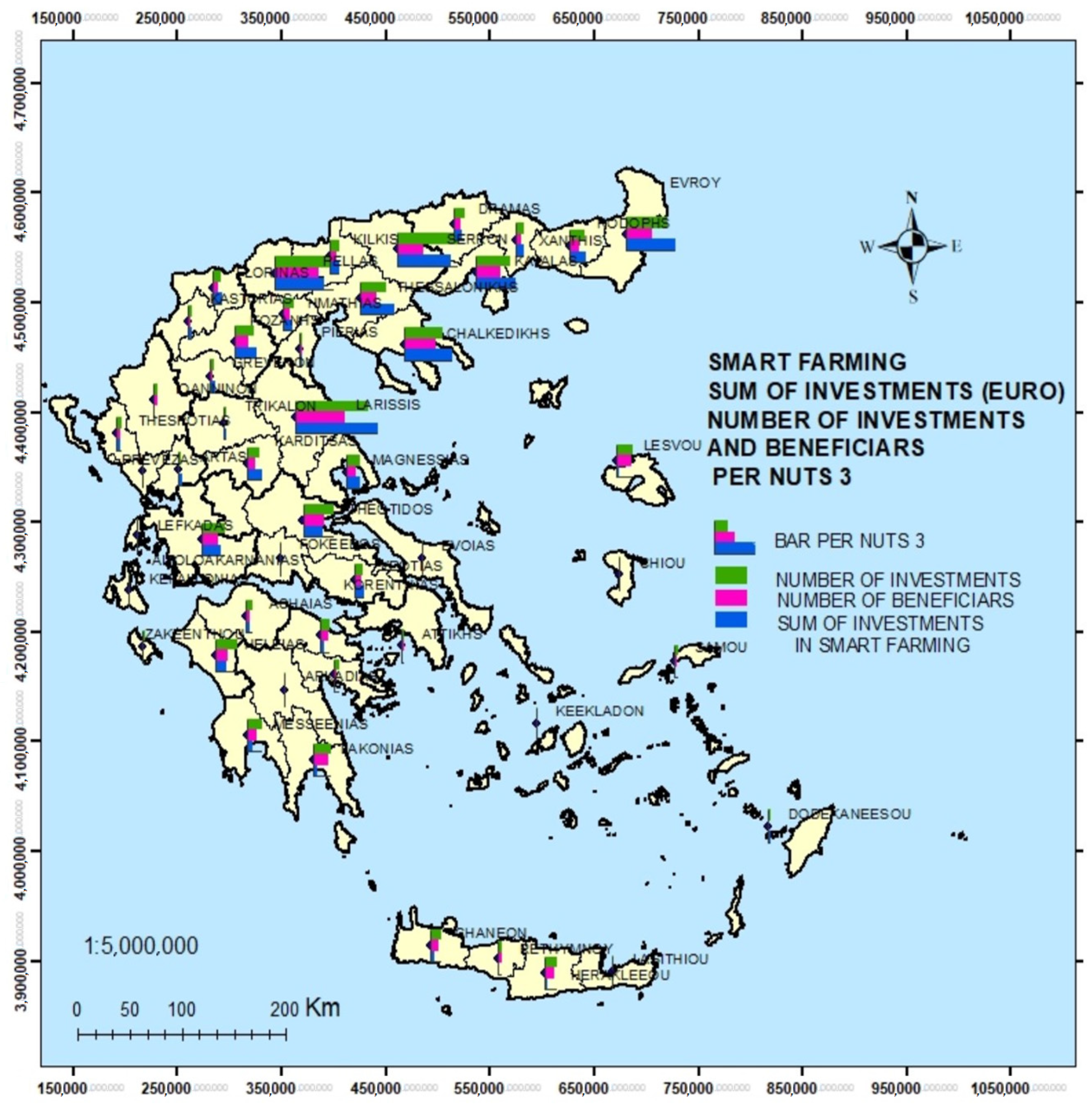
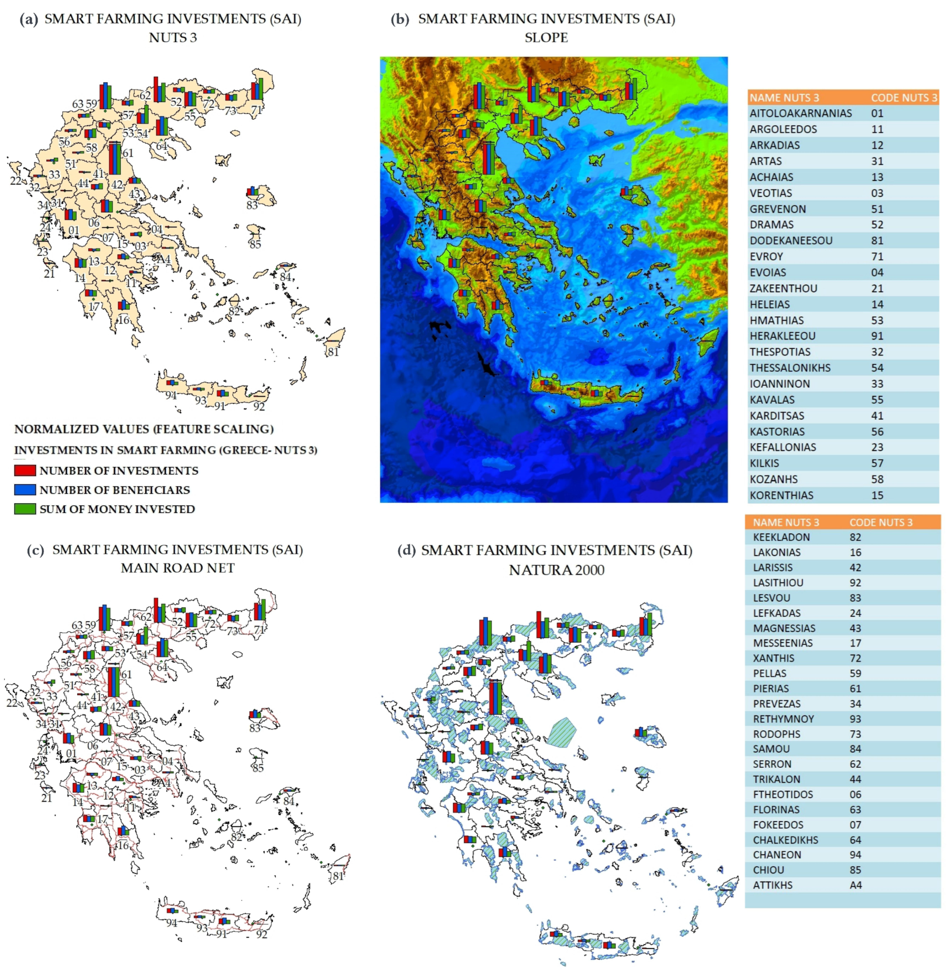
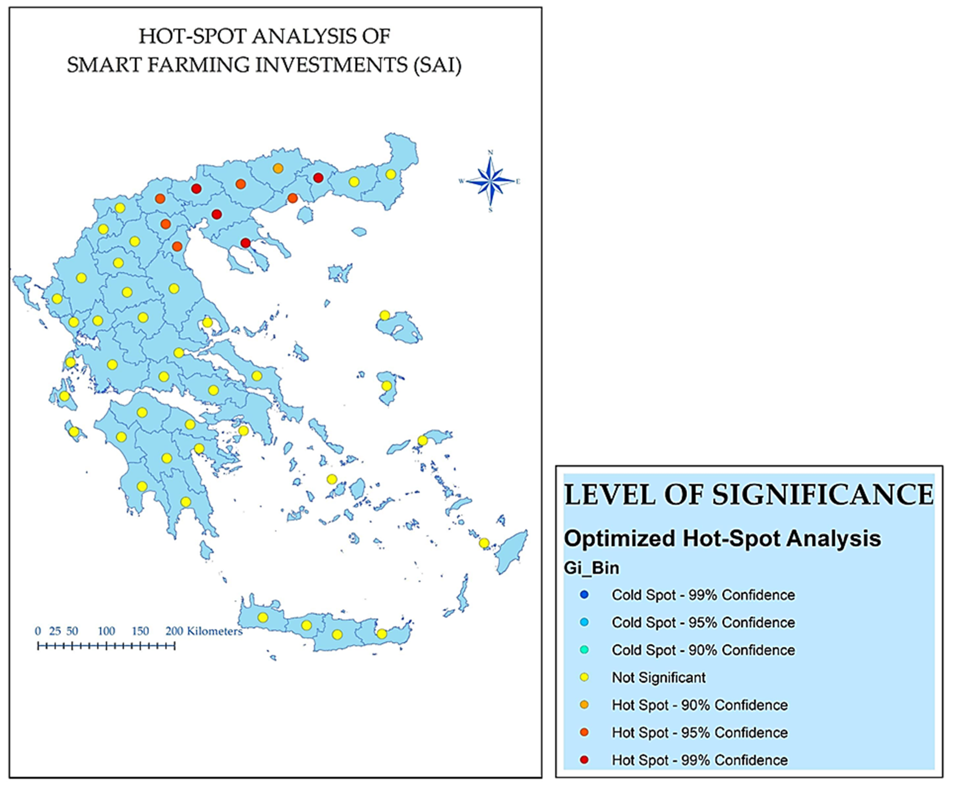
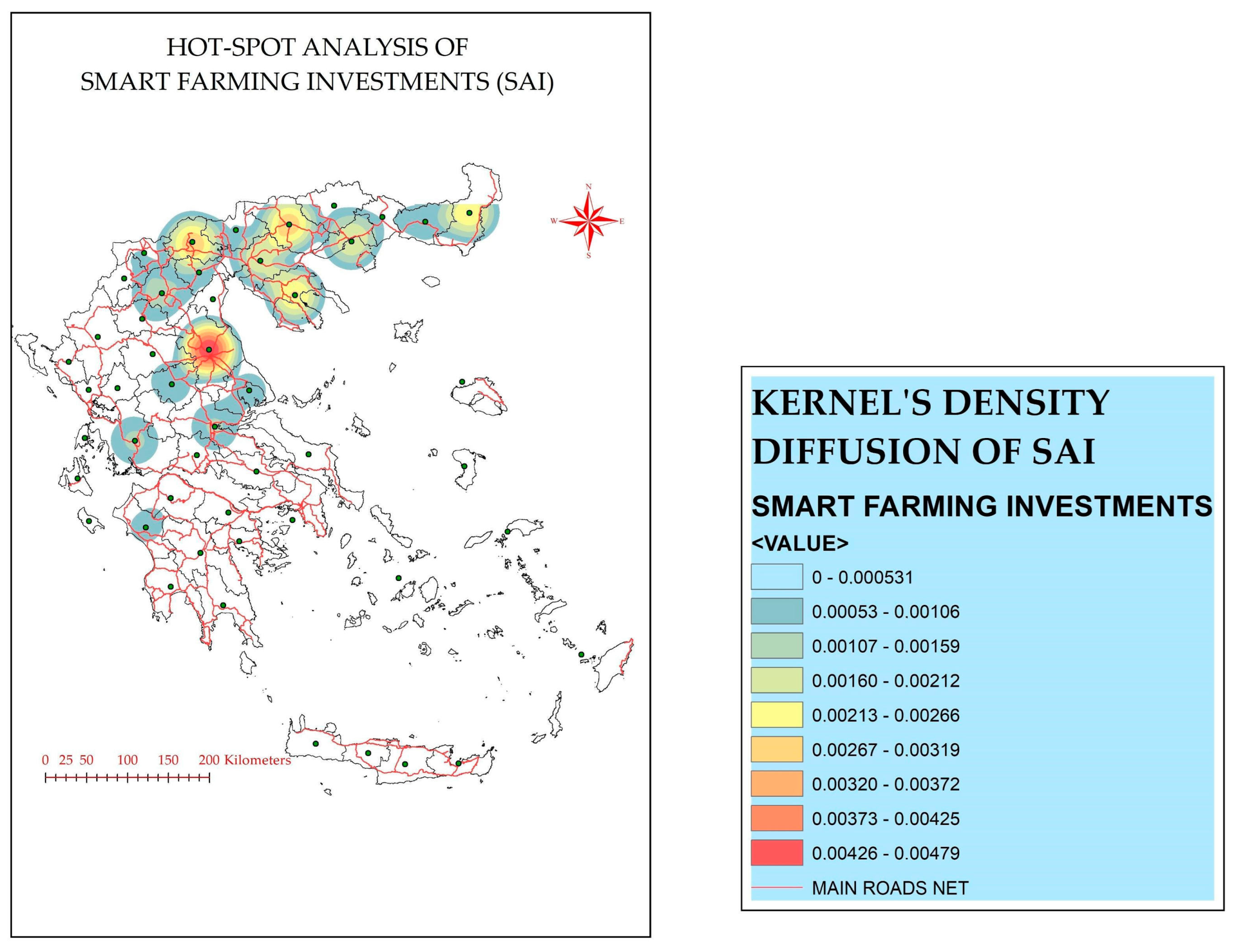
3.1. Spatial Patterns of Models’ Response Variables
3.2. Econometric Modeling
3.2.1. Model A—Total Agricultural Income—TAI
3.2.2. Model B—Smart Farming Investments—SFIs
3.2.3. Model C—RDP Investment Aid Schemes for Smart Agricultural Investments—AS-SAIs
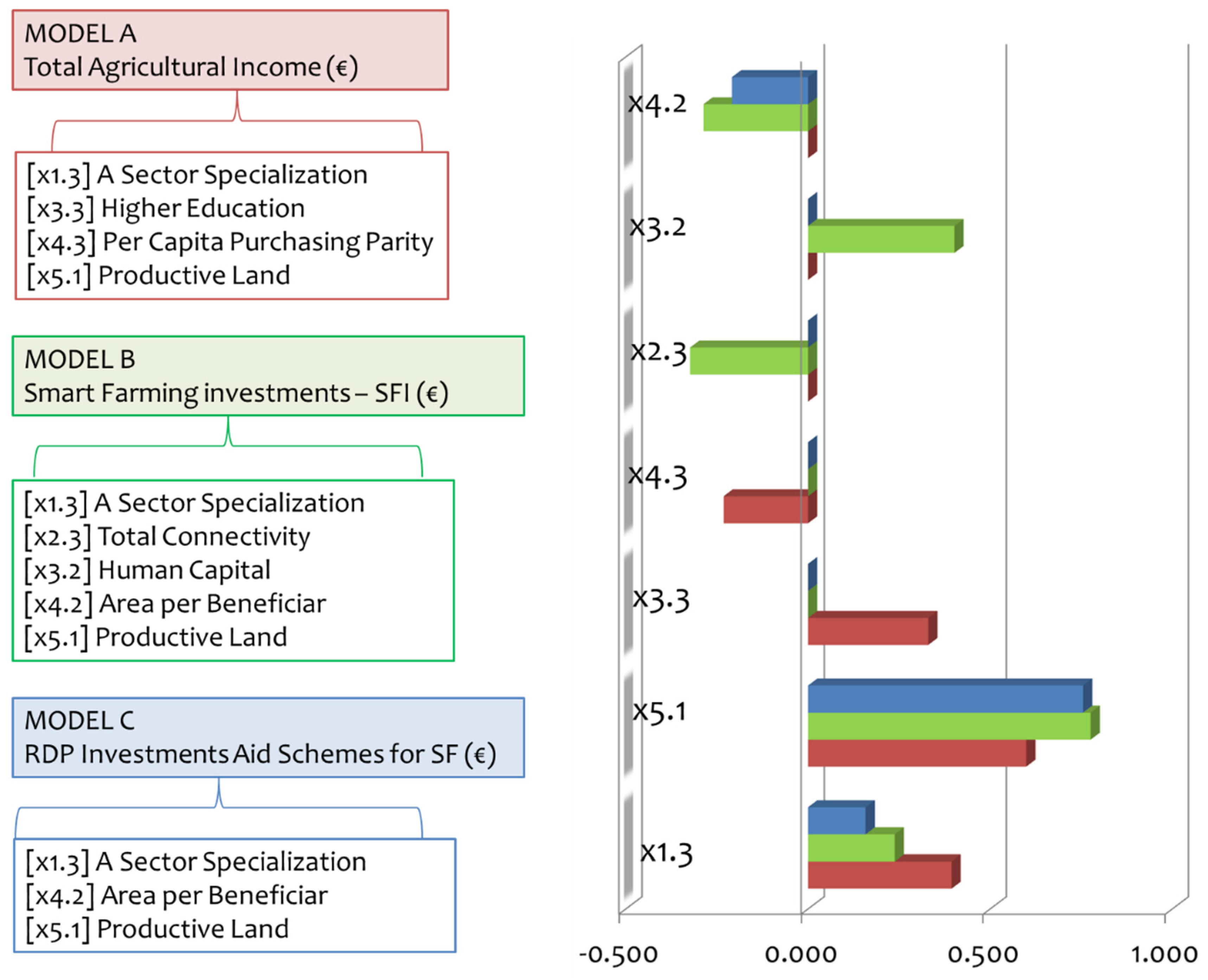
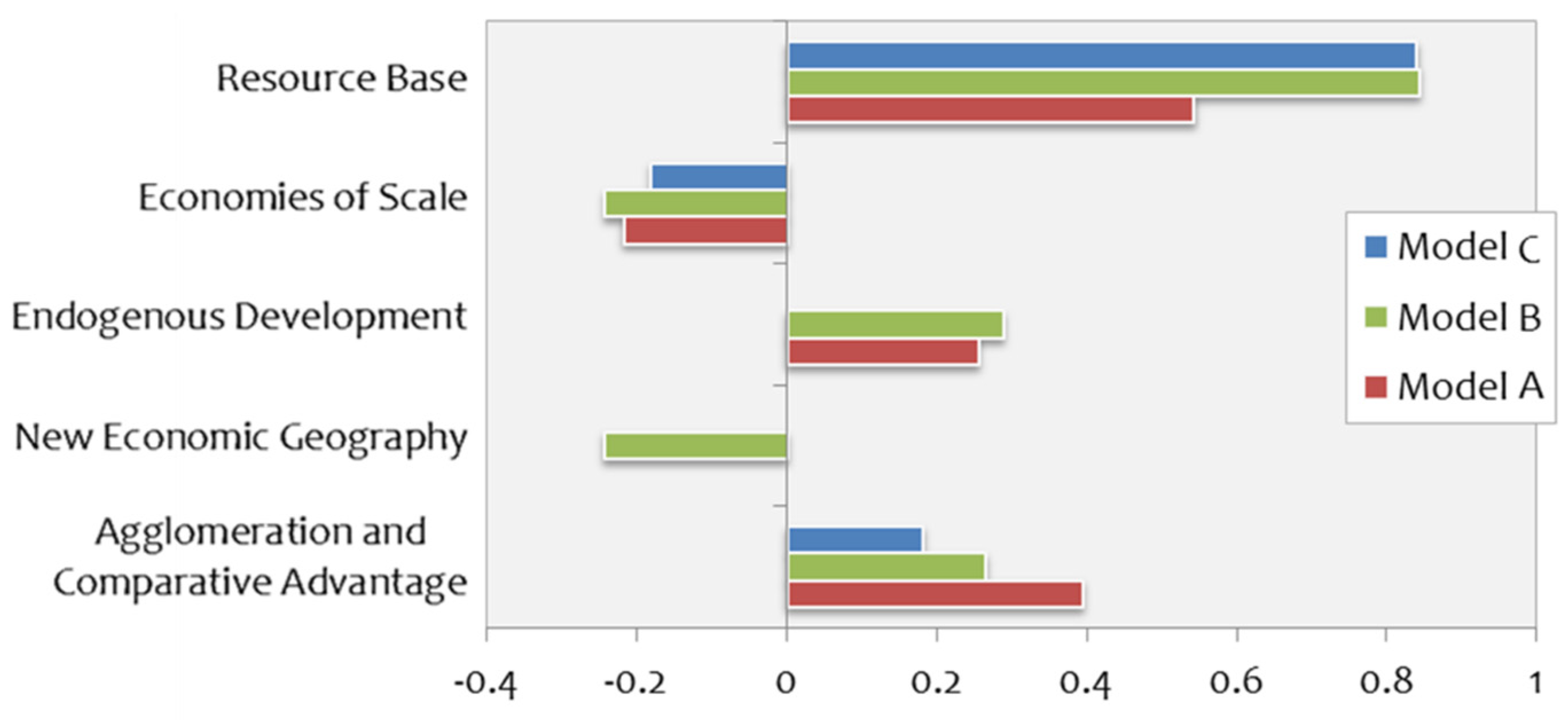
3.2.4. Model Comparisons
4. Conclusions
Author Contributions
Funding
Data Availability Statement
Acknowledgments
Conflicts of Interest
References
- Screpanti, E.; Zamagni, S. ‘Introduction’. In An Outline of the History of Economic Thought, 1st ed.; Online Ed; Field, D., Ed.; Oxford Academic: Online, 2003. [Google Scholar] [CrossRef]
- Childe, V.G. The Urban Revolution. Town Plan. Rev. 1950, 21, 3–17. Available online: http://www.jstor.org/stable/40102108 (accessed on 22 December 2022). [CrossRef] [Green Version]
- Smith, M.E.V. Gordon Childe and the Urban Revolution: A Historical Perspective on a Revolution in Urban Studies. Town Plan. Rev. 2009, 80, 3–29. Available online: http://www.jstor.org/stable/27715085 (accessed on 22 December 2022). [CrossRef] [Green Version]
- Rose, D.; Chilvers, J. Agriculture 4.0: Broadening responsible innovation in an era of smart farming. Front. Sustain. Food Syst. 2018, 2, 87. [Google Scholar] [CrossRef] [Green Version]
- Wolfert, A.; Ge, L.; Verdouw, C.; Bogaardt, M. Big data in smart farming- a review. Agric. Syst. 2017, 153, 69–80. [Google Scholar] [CrossRef]
- Basso, B.; Antle, J. Digital agriculture to design sustainable agricultural systems. Nat. Sustain. 2016, 3, 254–256. [Google Scholar] [CrossRef]
- Weersink, A.; Fraser, E.; Pannell, D.; Dunkan, E.; Rotz, S. Opportunities and challenges for big data in agricultural and environmental analysis 2018. Annu. Rev. Resour. Econ. 2018, 10, 19–37. [Google Scholar] [CrossRef]
- Balafoutis, A.; Beck, B.; Fountas, S.; Vangeyte, J.; Van der Wal, T.; Soto, I.; Gómez-Barbero, M.; Barnes, A.; Eory, V. Precision Agriculture Technologies Positively Contributing to GHG Emissions Mitigation, Farm Productivity and Economics. Sustainability 2017, 9, 1339. [Google Scholar] [CrossRef] [Green Version]
- El Bilali, H.; Allahyari, M.S. Transition towards sustainability in agriculture and food systems: Role of information and communication technologies. Inf. Process. Agric. 2018, 5, 456–464. [Google Scholar] [CrossRef]
- Lipper, L.; Thornton, P.; Cambel, B.; Torquebiau, E. Climate-smart agriculture for food security. Nat. Clim. Chang. 2014, 4, 1068–1072. [Google Scholar] [CrossRef]
- Asheim, B.T.; Smith, H.L.; Oughton, C. Regional Innovation Systems: Theory, Empirics and Policy. Reg. Stud. 2011, 45, 875–889. [Google Scholar] [CrossRef]
- MaCPherson, J.; Voglhuber-Slavinsky, A.; Olbrisch, M.; Schöbel, P.; Dönitz, E.; Mouratiadou, I.; Helming, K. Future agricultural systems and the role of digitalization for achieving sustainability goals: A review. Agron. Sustain. Dev. 2022, 42, 70. [Google Scholar] [CrossRef]
- Steinmueller, W.E. Understanding technical change as an evolutionary process: Richard R. Nelson,(North-Holland, Amsterdam, 1987). J. Econ. Behav. Organ. 1989, 11, 450–453. [Google Scholar] [CrossRef]
- Śledzik, K. Schumpeter’s View on Innovation and Entrepreneurship. SSRN Electron. J. 2013. [Google Scholar] [CrossRef]
- Smith, A. An Inquiry into the Nature and Causes of the Wealth of Nations, 1st ed.; W. Strahan: London, UK, 1776; Volume 1, Available online: https://books.google.gr/books?id=C5dNAAAAcAAJ&pg=PP7&redir_esc=y#v=onepage&q&f=false (accessed on 7 December 2022).
- Nayak, A.K.J.R. Economies of scope: Context of agriculture, small family farmers and sustainability. Asian J. Ger. Eur. Stud. 2018, 3, 2. [Google Scholar] [CrossRef] [Green Version]
- Phillips, P.; Ryan, C.; Karwandy, J.; Procyshyn, T.; Parchewski, J. The Saskatoon Agricultural Biotechnology Cluster. In Handbook of Research on Clusters: Theories, Policies and Case Studies; Karlsson, C., Ed.; Edward Elgar: Cheltenham, UK, 2008; pp. 233–252. [Google Scholar] [CrossRef]
- Somale, M. Comparative Advantage in Innovation and Production. Am. Econ. J. Macroecon. 2021, 13, 357–396. [Google Scholar] [CrossRef]
- Porter, M.E. The Competitive Advantage of Nations; Macmillan: London, UK, 1990; ISBN 9780029253618. [Google Scholar]
- Romer, P. Increasing Returns and Long-Run Growth. J. Political Econ. 1986, 94, 1002–1037. Available online: https://www.jstor.org/stable/i331956 (accessed on 10 February 2023). [CrossRef] [Green Version]
- Lucas, R. On the Mechanics of Economic Development. J. Monet. Econ. 1998, 22, 3–42. [Google Scholar] [CrossRef]
- Barro, R.; Sala-i-Martin, X. Two Sector Models of Endogenous Growth in Economic Growth, 2nd ed.; MIT Press: Cambridge, MA, USA, 2004; pp. 239–284. ISBN 0-262-02553-1. [Google Scholar]
- Millar, D. Endogenous development: Some issues of concern. Dev. Pract. 2014, 24, 637–647. [Google Scholar] [CrossRef]
- Marshall, A. Principles of Economics, 1st ed.; Macmillan: London, UK, 1890; Volume 1, Available online: https://archive.org/details/principlesecono00marsgoog/page/n8/mode/2up?view=theater (accessed on 7 December 2022).
- Hart, N. Marshall’s Theory of Value: The Role of External Economies. Camb. J. Econ. 1996, 20, 353–369. [Google Scholar] [CrossRef]
- Blomstrom, M.; Kokko, A. Multinational Corporations and Spillovers. J. Econ. Surv. 1998, 12, 247–277. [Google Scholar] [CrossRef]
- Capello, R. Regional growth and local development theories: Conceptual evolution over fifty years of regional science. Geogr. Econ. Soc. 2009, 11, 9–21. Available online: https://www.cairn.info/revue-geographie-economie-societe-2009-1-page-9.htm (accessed on 10 February 2023). [CrossRef] [Green Version]
- Krugman, P. Increasing Returns and Economic Geography. J. Political Econ. 1991, 99, 484–499. [Google Scholar] [CrossRef]
- Krugman, P.; Venables, A.J. Integration, specialization, and adjustment. Eur. Econ. Rev. 1996, 40, 959–967. [Google Scholar] [CrossRef] [Green Version]
- Fujita, M.; Thisse, J.-F. Economics of Agglomeration. J. Jpn. Int. Econ. 1996, 10, 339–378. Available online: http://www.casa.ucl.ac.uk/new-zipf/papers/fujita-thisse-agglom.pdf (accessed on 20 January 2023). [CrossRef] [Green Version]
- Gruber, S.; Soci, A. Agglomeration, Agriculture, and the Perspective of the Periphery. Spat. Econ. Anal. 2010, 5, 42–72. [Google Scholar] [CrossRef]
- Klerkx, L.; Jakku, E.; Labarthe, P. A review of social science on digital agriculture, smart farming and agriculture 4.0: New contributions and a future research agenda. NJAS—Wagening. J. Life Sci. 2019, 90, 100315. [Google Scholar] [CrossRef]
- Rogers, E.M. Diffusion of Innovations, 1st ed.; New York Free Press: New York, NY, USA, 1962. [Google Scholar] [CrossRef]
- Lebacq, T.; Baret, P.V.; Stilmant, D. Sustainability indicators for livestock farming: A review. Agron. Sustain. Dev. 2013, 33, 311–327. [Google Scholar] [CrossRef]
- Bathaei, A.; Štreimikienė, D. A Systematic Review of Agricultural Sustainability Indicators. Agriculture 2023, 13, 241. [Google Scholar] [CrossRef]
- Van Cauwenbergh, N.; Biala, K.; Charles, B.; Brouckaert, V.; Franchois, L.; Garcia Cidad, V.; Martin, H.; Erik, M.; Bart, M.; Reijnders, J. SAFE—A Hierarchical Framework for Assessing the Sustainability of Agricultural Systems. Agric. Ecosyst. Environ. 2007, 120, 229–242. [Google Scholar] [CrossRef]
- Peter, C.; Helming, K.; Nedel, C. Do greenhouse gas emission calculations from energy crop cultivation reflect actual agricultural management practices?—A review of carbon footprint calculators. Renew. Sustain. Energy Rev. 2017, 67, 461–476. [Google Scholar] [CrossRef] [Green Version]
- Marandure, T.; Dzama, K.; Bennett, J.; Makombe, G.; Chikwanha, O.; Mapiye, C. Farmer challenge-derived indicators for assessing sustainability of low-input ruminant production systems in sub-Saharan Africa. Environ. Sustain. Indic. 2020, 8, 100060. [Google Scholar] [CrossRef]
- Lampridi, M.G.; Sorensen, C.G.; Bochtis, D. Agricultural Sustainability: A review of Concepts and Methods. Sustainability 2019, 11, 5120. [Google Scholar] [CrossRef] [Green Version]
- Polyzos, S. Regional Development, 2nd ed.; Kritiki Publications: Athens, Greece, 2019. (In Greek) [Google Scholar]
- Polyzos, S. Urban Development; Kritiki Publications: Athens, Greece, 2015. (In Greek) [Google Scholar]
- Sdrolias, L.; Semos, A.; Mattas, K.; Tsakiridou, E.; Michailides, A.; Partalidou, M.; Tsiotas, D. Assessing the agricultural sector’s resilience to the 2008 economic crisis: The case of Greece. Agriculture 2022, 12, 174. [Google Scholar] [CrossRef]
- Tsiotas, D.; Tselios, V. Measuring the Interaction between the Interregional Accessibility and the Geography of Institutions: The case of Greece. In Economies, Institutions, and Territories: Dissecting Nexuses in a Changing World (The Dynamics of Economic Space); Storti, L., Urso, G., Reid, N., Eds.; Routledge: New York, NY, USA, 2023; pp. 269–294. [Google Scholar] [CrossRef]
- Walpole, R.E.; Myers, R.H.; Myers, S.L.; Ye, K. Probability & Statistics for Engineers & Scientists, 9th ed.; Prentice Hall Publications: New York, NY, USA, 2012; Available online: https://math.buet.ac.bd/public/faculty_profile/files/835598806.pdf (accessed on 7 December 2022).
- Norusis, M. IBM SPSS Statistics 19.0 Guide to Data Analysis; Prentice Hall: Hoboken, NJ, USA, 2011; ISBN 9780321748416. [Google Scholar]
- Tsiotas, D.; Papadimopoulos, I.; Aspridis, G.; Sdrolias, L. Socioeconomic determinants in the topology of spatial networks: Evidence from the interregional road network in Greece. Theor. Empir. Res. Urban Manag. 2020, 15, 5–28. [Google Scholar]
- IBM SPSS Statistics 26 on Line Guide. Available online: https://www.ibm.com/docs/en/spss-statistics/26.0.0 (accessed on 20 January 2023).
- ESRI (Environmental Systems Research Institute, Inc.). (n.d.) ArcGIS How Hot Spot Analysis (Getis-Ord Gi*) Works. Available online: http://resources.arcgis.com/en/help/main/10.2/index.html#/How_Hot_Spot_Analysis_Getis_Ord_Gi_works/005p00000011000000/ (accessed on 2 February 2023).
- Czyżewski, B.; Polcyn, J.; Brelik, A. Political orientations, economic policies, and environmental quality: Multi-valued treatment effects analysis with spatial spillovers in country districts of Poland. Environ. Sci. Policy 2021, 128, 1–13. [Google Scholar] [CrossRef]
- ESRI (Environmental Systems Research Institute, Inc.). (n.d.) ArcGIS How Kernel Density Works. Available online: https://pro.arcgis.com/en/pro-app/latest/tool-reference/spatial-analyst/how-kernel-density-works.htm (accessed on 20 January 2023).
- Michailidis, A.; Samarthrakis, B.; Xatzitheodoridis, F.; Loizou, E. Adoption-diffusion of precision agriculture: Comparative analysis among the Greek Regions. In Innovative Applications of Information Technology in the Agricultural Sector and the Environment; Arambatzidis, G., Samathrakiis, B., Matopoulos, A., Mpournaris, T., Eds.; Vol 3 of the Scientific papers of the Hellenic Association for Information and Communication Technologies in agriculture Food and Environment (HAICTA); Brunch of Northern and Central Greece: Thessaloniki, Greece, 2010. [Google Scholar]
- Mourtzinis, S.; Fountas, S.; Gemtos, T. Perspective of Greek farmers for precision agriculture. In Proceedings of the 5th National Congress of Agricultural Engineering, Larisa, Greece, 18–20 October 2007; Volume 185, pp. 850–857. [Google Scholar]
- Gatrell, A.C.; Bailey, T.C.; Diggle, P.J.; Rowlingson, B.S. Spatial Point Pattern Analysis and Its Application in Geographical Epidemiology. Trans. Inst. Br. Geogr. 1996, 21, 256. [Google Scholar] [CrossRef]
- Brunsdon, C. Estimating probability surfaces for geographical point data: An adaptive kernel algorithm. Comput. Geosci. 1995, 21, 877–894. [Google Scholar] [CrossRef]
- Tsiotas, D. A network-based algorithm for computing Keynesian income multipliers in multiregional systems. Reg. Sci. Inq. 2022, 14, 25–46. Available online: http://www.rsijournal.eu/ARTICLES/December_2022/2.pdf (accessed on 10 February 2023).
- Christofakis, M.; Padaskalopoulos, A. The Growth Poles strategy in regional planning: The recent experience of Greece. Theor. Empir. Res. Urban Manag. 2011, 6, 5–20. [Google Scholar]
- Erling, L.; Ken, C.; Xiaojian, L.; Xinyue, Y.; Leipnik, M. Analyzing Agricultural Agglomeration in China. Sustainability 2017, 9, 313. [Google Scholar] [CrossRef] [Green Version]
- Czyżewski, A.; Smędzik-Ambroży, K. Specialization and diversification of agricultural production in the light of sustainable development. J. Int. Stud. 2015, 8, 63–73. [Google Scholar] [CrossRef]
- Wang, X.-B.; Cai, D.-X.; Hoogmoed, W.; Oenema, O.; Perdok, U. Potential Effect of Conservation Tillage on Sustainable Land Use: A Review of Global Long-Term Studies. Pedosphere 2006, 16, 587–595. [Google Scholar] [CrossRef]
- Esmaeilpoorarabi, N.; Yigitcanlar, T.; Guaralda, M. Place quality in innovation clusters: An empirical analysis of global best practices from Singapore, Helsinki, New York, and Sydney. Cities 2018, 74, 156–168. [Google Scholar] [CrossRef] [Green Version]
- Scott, A.J. Emerging cities of the third wave. City 2011, 15, 289–321. [Google Scholar] [CrossRef]
- Schreyer, P.; Koechlin, F. Purchasing Power Parities—Measurements and Uses. Statics Brief, Statistics Directorate OECD 2002, vol 3. Available online: https://www.oecd.org/sdd/prices-ppp/2078177.pdf (accessed on 10 February 2023).
- Škare, M.; Lacmanović, S. Human capital and economic growth: A review essay. Amfiteatru Econ. J. 2015, 17, 735–760. Available online: https://www.econstor.eu/handle/10419/168945 (accessed on 20 January 2023).
- Koutridi, E.; Christopoulou, O.; Duquenne, M.-N. Perceptions and Attitudes of Greek farmers towards adopting Precision Agriculture: Case Study Region of Central Greece. In Multicriteria Analysis in Agriculture: Current Trends and Recent Applications; Special Issue; Barbel, J., Bournaris, T., Manos, B., Matsatsinis, N., Viaggi, D., Eds.; Springer Nature: Cham, Switzerland, 2018; pp. 223–266. ISSN 2366-0031. ISBN 978-3-319-76928-8. [Google Scholar] [CrossRef]
- Lee, R. Chapter 2—Macroeconomics, Aging, and Growth. In Handbook of the Economics of Population Aging; Piggott, J., Woodland, A., Eds.; Elservier Amsterdam the Netherlands North-Holland: Amsterdam, The Netherlands, 2016; Volume 1, pp. 59–118. ISSN 2212-0076. ISBN 9780444634054. [Google Scholar] [CrossRef] [Green Version]
- Takahashi, T. On the economic geography of an aging society. Reg. Sci. Urban Econ. 2022, 95, 103798. [Google Scholar] [CrossRef]
- Krugman, P.; Livas Elizondo, R. Trade policy and the Third World metropolis. J. Dev. Econ. 1996, 49, 137–150. [Google Scholar] [CrossRef] [Green Version]
- Fankhaeser, S.; Sehlleier, F.; Stern, N. Climate change, innovation and jobs. Clim. Policy 2008, 8, 421–429. [Google Scholar] [CrossRef]
- Denton, F.; Wilbanks, T.J.; Abeysinghe, A.C.; Burton, I.; Gao, Q.; Lemos, M.C.; Masui, T.; O’Brien, K.L.; Warner, K. Climate-resilient pathways: Adaptation, mitigation, and sustainable development. In Climate Change Impacts, Adaptation, and Vulnerability; Part A: Global and Sectoral Aspects. Contribution of Working Group II to the Fifth Assessment Report of the Intergovernmental Panel on Climate Change; Field, C.B., Barros, V.R., Dokken, D.J., Mach, K.J., Mastrandrea, M.D., Bilir, T.E., Chatterjee, M., Ebi, K.L., Estrada, Y.O., Genova, R.C., et al., Eds.; Cambridge University Press: Cambridge, UK; New York, NY, USA, 2014; pp. 1101–1131. Available online: https://www.ipcc.ch/site/assets/uploads/2018/02/WGIIAR5-Chap20_FINAL.pdf (accessed on 20 January 2023).
- Kuehne, G.; Llewellyn, R.; Pannell, D.J.; Wilkinson, R.; Dolling, P.; Ouzman, J.; Ewing, M. Predicting Farmer Uptake of New Agricultural Practices: A Tool for Research, Extension and Policy. Agric. Syst. 2017, 156, 115–125. [Google Scholar] [CrossRef]
- Weersink, A.; Fulton, M. Limits to Profit Maximization as a Guide to Behavior Change. Appl. Econ. Perspect. Policy 2020, 1, 67–79. [Google Scholar] [CrossRef] [Green Version]


| Category 1 | Subcategory 1 | Name of Category |
|---|---|---|
| 1 | 11–16 | GPS Vehicle Guidance |
| 2 | 21–28 | Farm Management Information Systems |
| 3 | 36–39 & 311–312 & 320 | Plant production facility equipment |
| 4 | 48–49 & 410–415 | Variable Rate Crop Spraying Systems |
| 5 | 531 & 533 | Variable Rate Applicators |
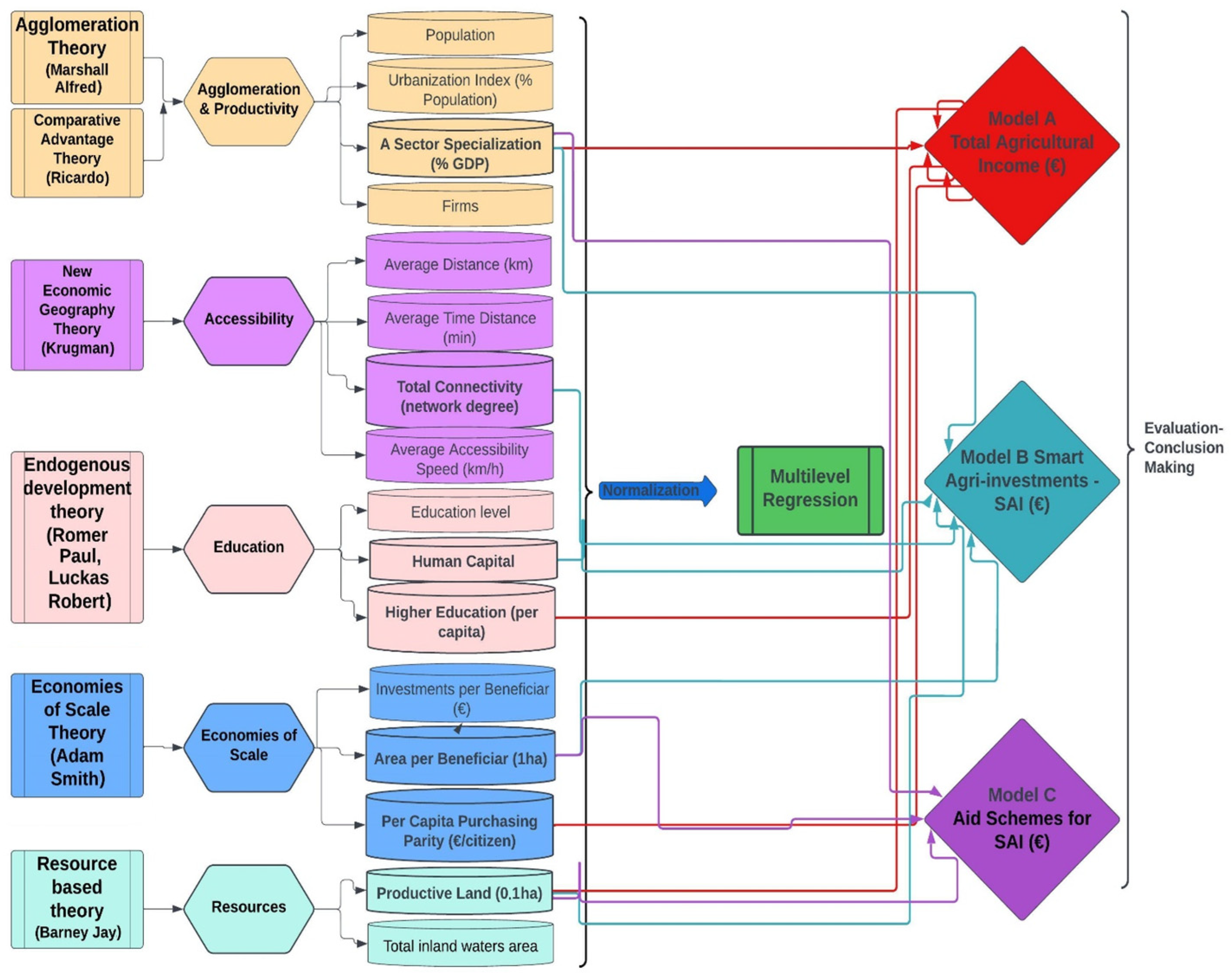
| Theoretical Context | Representatives | Code | Description | Source |
|---|---|---|---|---|
| Agglomeration Theory and Comparative Advantage Theory | Population | ×1.1 | The population of each prefecture (NUTS III), according to the 2011 national census. | [40] |
| Urbanization Index (% Population) | ×1.2 | Defined by the share of a prefecture’s capital city to the prefecture’s population. | [41] | |
| A Sector Specialization (% GDP) | ×1.3 | The share of % GDP attributed to agriculture (primary sector). | [42] | |
| Firms | ×1.4 | The number of firms registered in each prefecture. | [40] | |
| New Economic Geography Theory | Average Distance (km) | ×2.1 | The average kilometric distance of each prefecture to the others. | [43] |
| Average Time Distance (min) | ×2.2 | The average time distance (measured in minutes) of each prefecture to the others. | [43] | |
| Total Connectivity (network degree) | ×2.3 | Composite index measuring the aggregated average degree of multimodal transportation networks of Greek prefectures. | [43] | |
| Average Accessibility Speed (km/h) | ×2.4 | The average speed (km/h) required to access a prefecture. | [43] | |
| Endogenous Development Theory | Education level | ×3.1 | Composite index measuring the level of Education in a prefecture. | [40] |
| Human Capital | ×3.2 | Composite index measuring the level of education of labor force (labor production coefficient) in a prefecture. | [40] | |
| Higher Education (per capita) | ×3.3 | A number showing the population corresponding to one person with higher education (per capita) | [40] | |
| Economies of Scale Theory | Investments per Beneficiary (€) | ×4.1 | The total budget of investments corresponding to a beneficiary (€), per prefecture. | Aggregated from data |
| Area per Beneficiary (1 ha) | ×4.2 | The total area corresponding to a beneficiary (1 ha), per prefecture. | Aggregated from data | |
| Per Capita Purchasing Parity (€/citizen) | ×4.3 | The per capita purchasing parity (€/citizen) of a prefecture | [40] | |
| Resource Base Theory | Productive land (0.1 ha) | ×5.1 | The total productive land area, per prefecture (0.1 ha). | [40] |
| Total inland waters area | ×5.2 | The total inland waters area, per prefecture. | [40] |
| Model A | Model Summary | Coefficients | |||||||||
|---|---|---|---|---|---|---|---|---|---|---|---|
| Dependent Variable: Total Agricultural Income (EUR) | R | R2 | R2Adj | Std. Error of the Estimate | Unstandardized Coefficients | Standardized Coefficients | 95% Confidence Interval for B | ||||
| 0.732 | 0.536 | 0.496 | 0.170159 | B | Std. Error | Beta | t | Sig. | Lower Bound | Upper Bound | |
| Independent Variables | Constant | −0.149 | 0.094 | −1.591 | 0.118 | −0.337 | 0.039 | ||||
| A Sector Specialization (% GDP) | 0.394 | 0.128 | 0.394 | 3.072 | 0.004 | 0.136 | 0.652 | ||||
| Higher Education (per capita) | 0.330 | 0.169 | 0.255 | 1.954 | 0.057 | −0.010 | 0.670 | ||||
| Per Capita Purchasing Parity (EUR/citizen) | −0.232 | 0.121 | −0.218 | −1.921 | 0.061 | −0.474 | 0.011 | ||||
| Productive Land (1 ha) | 0.599 | 0.110 | 0.543 | 5.098 | 0.000 | 0.338 | 0.779 | ||||
| Model B | Model Summary | Coefficients | |||||||||
| Dependent Variable: Smart Farming Investments—SFI (EUR) | R | R2 | R2Adj | Std. Error of the Estimate | Unstandardized Coefficients | Standardized Coefficients | 95% Confidence Interval for B | ||||
| 0.869 | 0.755 | 0.728 | 0.1118427 | B | Std. Error | Beta | t | Sig. | Lower Bound | Upper Bound | |
| Independent Variables | Constant | −0.023 | 0.050 | −0.461 | 0.647 | −0.124 | 0.078 | ||||
| A Sector Specialization (% GDP) | 0.238 | 0.084 | 0.265 | 2.827 | 0.007 | 0.068 | 0.407 | ||||
| Total Connectivity (network degree) | −0.324 | 0.192 | −0.244 | −1.685 | 0.099 | −0.712 | 0.063 | ||||
| Human Capital | 0.402 | 0.214 | 0.288 | 1.878 | 0.067 | −0.029 | 0.834 | ||||
| Area per Beneficiary (1 ha) | −0.287 | 0.104 | −0.243 | −2.756 | 0.008 | −0.496 | −0.077 | ||||
| Productive Land (1 ha) | 0.776 | 0.076 | 0.843 | 10.196 | 0.000 | 0.623 | 0.929 | ||||
| Model C | Model Summary | Coefficients | |||||||||
| Dependent Variable: RDP Investments Aid Schemes for SF (EUR) | R | R2 | R2Adj | Std. Error of the Estimate | Unstandardized Coefficients | Standardized Coefficients | 95% Confidence Interval for B | ||||
| 0.853 | 0.728 | 0.711 | 0.1125364 | B | Std. Error | Beta | t | Sig. | Lower Bound | Upper Bound | |
| Independent Variables | Constant | −0.037 | 0.040 | −0.924 | 0.360 | −0.116 | 0.043 | ||||
| A Sector Specialization (% GDP) | 0.158 | 0.070 | 0.181 | 2.256 | 0.029 | 0.029 | 0.299 | ||||
| Area per Beneficiary (1 ha) | −0.209 | 0.095 | −0.182 | −2.206 | 0.032 | 0.032 | −0.018 | ||||
| Productive land (1 ha) | 0.755 | 0.074 | 0.840 | 10.232 | 0.000 | 0.000 | 0.903 | ||||
Disclaimer/Publisher’s Note: The statements, opinions and data contained in all publications are solely those of the individual author(s) and contributor(s) and not of MDPI and/or the editor(s). MDPI and/or the editor(s) disclaim responsibility for any injury to people or property resulting from any ideas, methods, instructions or products referred to in the content. |
© 2023 by the authors. Licensee MDPI, Basel, Switzerland. This article is an open access article distributed under the terms and conditions of the Creative Commons Attribution (CC BY) license (https://creativecommons.org/licenses/by/4.0/).
Share and Cite
Koutridi, E.; Tsiotas, D.; Christopoulou, O. Examining the Spatial Effect of “Smartness” on the Relationship between Agriculture and Regional Development: The Case of Greece. Land 2023, 12, 541. https://doi.org/10.3390/land12030541
Koutridi E, Tsiotas D, Christopoulou O. Examining the Spatial Effect of “Smartness” on the Relationship between Agriculture and Regional Development: The Case of Greece. Land. 2023; 12(3):541. https://doi.org/10.3390/land12030541
Chicago/Turabian StyleKoutridi, Evagelia, Dimitrios Tsiotas, and Olga Christopoulou. 2023. "Examining the Spatial Effect of “Smartness” on the Relationship between Agriculture and Regional Development: The Case of Greece" Land 12, no. 3: 541. https://doi.org/10.3390/land12030541