Open Habitats under Threat in Mountainous, Mediterranean Landscapes: Land Abandonment Consequences in the Vegetation Cover of the Thessalian Part of Mt Agrafa (Central Greece)

Abstract

Land abandonment is one of the main drivers of land use/land cover (LULC) change across Europe, which has already led to a significant loss of open habitats, threatening species hosted in them. We investigated LULC changes for a period of 70 years in a mountainous area of central Greece (Mt Agrafa) by mapping its land cover for the years 1945, 1996 and 2015, calculating transition matrices of land cover classes and performing intensity analysis at different levels. Subareas of the study area, with different population trends, were compared in regard to their LULC change trends. Possible drivers of LULC changes were explored by means of Random Forest modeling, and landscape metrics were calculated to assess their trends. Our results showed great changes in LULC class cover, significant shrinkage of open habitats, accelerated rates of change in the recent period and no differences in LULC change patterns in relation to different population trends. Variables expressing favorability of ecological conditions for forest establishment or probability of farmland abandonment were found as more important drivers of the spatiotemporal distribution of LULC classes, while landscape metrics revealed certain trends. Our main conclusion is that land abandonment and the subsequent vegetation succession are going through a semifinal stage, before their completeness and the almost absolute dominance of the forest, and repopulation of the countryside cannot unconditionally ensure any halting effect on the land abandonment process.

1. Introduction

The investigation of changes of land use and land cover across different spatial and temporal scales has been of great scientific interest during the last decades, with land cover referring to the visible surface of land (e.g., forests, shrublands, wetlands, agricultural), while land use refers to the socioeconomic purpose of human activities on the landscape (e.g., recreation, forestry, agriculture). Land abandonment is one of the main trajectories of land use/land cover (LULC) change across Europe [1] and has led to a significant reduction in agricultural land over the past few decades, mainly in mountainous regions of the Mediterranean [2,3,4]. In recent years, there is a growing concern in European Union (EU) about this phenomenon, as it is estimated that around 30% of agricultural areas are under moderate risk of land abandonment by 2030 [5]. Although the amount of total abandoned agricultural land throughout the EU is expected to reach the 3% of the total current agricultural area by 2030, it is estimated that several countries will be affected by significantly higher levels of land abandonment, with Greece having more than 70% of its agricultural land under at least moderate risk of abandonment [6]. In mountainous regions, this risk is three times higher than in non-mountainous regions [7], highlighting the importance that agricultural land abandonment will have on these ecosystems [6,8].

Effects of land abandonment can be positive under certain cases, e.g., through the provision of opportunities for the recovery of disturbed ecosystems [9,10], restoration of historical vegetation [11] or improvement of soil conditions and water regulation [10]. Nevertheless, the negative effects of abandonment are usually more prominent and include landscape and vegetation homogenization [10], accompanied with a subsequent loss of biodiversity occurring in the semi-natural habitats that are gradually lost [12], alteration of soil properties and ecosystem processes [10,11], as well as an increase in wildfire frequency and severity [13]. The EU has drawn particular attention to the potential negative effects of land abandonment on habitats and biodiversity connected to agricultural activities (grasslands and shrubs) [14], since the European countryside and therefore agricultural biodiversity and habitat types have been largely shaped by the application of traditional land uses over millennia [15,16]. The cessation of such activities results in the initiation of the process of secondary succession of vegetation [17,18], which starts immediately after land abandonment [19] and is characterized by the replacement of open habitats’ vegetation by shrubland/woodland vegetation and finally by forest vegetation [20,21]. Particularly in the Mediterranean biogeographic region, the loss of open habitats and landscape homogenization are expected to subsequently lead to decline of a great number of narrowly distributed, endemic or threatened species inhabiting these grasslands [22].

The main causal drivers of land abandonment within the EU include both socioeconomic and environmental factors. On one hand, socioeconomic drivers include extensive urbanization due to major economic changes at a local or regional level [5], the low competitive ability of small-scale farmers [12] and the intensification of agricultural activities on more productive lands leading to increasing imports of agricultural products from other regions [23]. On the other hand, complexity of landscape topography, soil characteristics (e.g., physical properties, water holding capacity, pH) as well as climatic conditions [10] are among the main ecological drivers of land abandonment. As a general pattern, agricultural abandonment within Europe is observed in areas with unfavorable cultivation conditions, such as areas with low productivity, in remote and mountainous localities and in areas where soil erosion is prevalent [10,12].

The particularly high percentage of areas under moderate and high risk of abandonment in Greece is related to factors including general economic conditions, social factors (e.g., occupation or way of living preferences), as well as characteristics of the primary sector (concerning agricultural practices or market characteristics) [6]. Moreover, biophysical factors such as high-altitude areas, islands and areas subject to drought contribute substantially to this high abandonment risk [6]. An additional potential driver of land abandonment, which has received special attention due to its great importance, is depopulation. More specifically, the slowing down of the population growth of Europe and the rural population decline during the last decades are considered at least partly responsible for shrinkage of agricultural land at the regional scale [12].

The aim of the present study was to investigate the LULC changes in a mountainous area of central Greece for a period of 70 years, and specifically on the basis of data from three years, namely, 1945, 1996 and 2015. The study area is composed of municipal districts with different population trends in time, giving us the ability to investigate if such different trends have led to different LULC change patterns. Transition matrices between LULC classes as well as their change rate were calculated for the whole study area as well as for the two subareas distinguished on the basis of their distinct population trends. Furthermore, we explored the impact of ecological and socioeconomic variables on the probability of each LULC class occurrence in the landscape and calculated certain landscape metrics for the different years studied. The questions addressed in this study are the following:

(1)

Which LULC classes were submitted to changes in time and to what extent, and how were the transitions between the LULC classes directed?

(2)

What was the rate of change (transitions) between LULC classes and was rate was differentiated in time or between classes or transition types?

(3)

Were there different patterns in LULC change and rate between the municipal districts with different population trends?

(4)

Which ecological or socioeconomic factors had important effects on the probability of each LULC class occurrence in the landscape and how did they affect the probability of each class?

(5)

How did certain landscape aspects change in time and for each LULC class?

2. Materials and Methods

2.1. Study Area

The study area is located at the Thessalian part of Mt Agrafa (central Greece), which is located within the Southern Pindus floristic region of Greece [24]. Its total area covers 112.38 km² and its elevation ranges from 456 m to 1.525 m, with a mean altitude of 920 m. Based on the map of Beck et al. [25], the climate of more than half of the study area (≈60%) is “Warm-summer Mediterranean climate” (Csb) and for the rest is “Hot-summer Mediterranean climate” (Csa), while according to the data obtained from the CHELSA Version 2.1 dataset [26] for the period 1981–2010, its average air temperature is 11.1 °C and the annual average precipitation is 999 mm. The geological substrate of the study area comprises mainly shale and flysch [27].

The potential natural vegetation of the study area includes two forest types, namely the “South and east Balkan colline to montane (mixed) Balkan oak forests” and the “Hellenic beech and fir-beech forests” [28]. The former vegetation type is mainly represented by Quercus frainetto Ten. forests and covers more than 78% of the study area, while the latter is represented by Abies borisii-regis Mattf. forests, occurring at the highest altitudinal zone of the study area [28]. Within both of the abovementioned vegetation zones, ecological factors as well as human-induced disturbances (e.g., agricultural activities, tourist and recreational facilities, urban structures) might have prevented the establishment of potential vegetation types, leading to a mosaic landscape of different vegetation stages of secondary succession, such as abandoned fields, semi-natural grasslands (grasslands occurring in areas having forests as natural potential vegetation but which are covered by open habitats’ vegetation because of long-term human-induced disturbances), shrublands and degraded forests. The study area includes parts from 13 municipal districts of the Karditsa regional unit (Figure 1), while it historically includes only small-to-medium-sized villages.

Our study was conducted for a 70-year period, from 1945 to 2015, and the extent and borders of the study area were chosen so as to include areas of the sub-mountainous and mountainous zone where human agricultural activities were traditionally practiced continuously or intermittently during these years. To identify such areas, maps of a National Cadastre project were used to document the transitions between woodland and agricultural land from 1945 to date. Visual interpretations of these maps revealed the main areas where major LULC changes have taken place over the last few decades. Furthermore, interviews were conducted with local residents to find areas with the abovementioned characteristics. In general, our study area was constituted by the villages and their current and former cultivated or pasture land, while we avoided extended remote areas with rough topography, which were forested already since 1945, as well as areas with subalpine vegetation (where climatic and soil conditions cannot support forest growth) occurring above 1500–1600 m within the general study area.

Another criterion for selecting the study area and subareas was their proximity to Lake Plastiras. This lake is artificial (it is also called Tavropos Reservoir) and was created by the construction of a dam at Tavropos (Megdovas) River in 1960. The surface area of the lake is 22.4 km². The rationale for using such a criterion is based on the fact that although the total population of the study area has been reduced from 11,249 inhabitants in 1940 to 8401 in 2011 (reduction of 25%), the municipal districts in the study area followed two different patterns concerning the trend of their population size (Figures S1 and S2). The municipal districts around the lake experienced an initial reduction of their population until 1980 or 1990, but afterwards their population increased and in 2011 reached or exceeded the one they had in 1940 (Figures S1 and S2). These municipal districts had in 2011 the same total population size as that in 1940. On the other hand, the municipal districts away from Lake Plastiras experienced a more or less continuous reduction of their population during the study period and in 2011 the total sum of their inhabitants was about the one-third of that in 1940 (Figures S1 and S2). We applied such a criterion to be able to compare LULC changes between areas of different population trends in time and to test certain related hypotheses.

2.2. Land Cover Mapping

LULC change in the study area was investigated for a period of 70 years and specifically from 1945 to 2015. Land cover was mapped in three time points, and specifically 1945, 1996 and 2015, on the basis of orthophotos provided by Hellenic Cadastre for the years 1945 (pixel size 1 m) and 2015 (pixel size 0.25 m) and orthophotos of 1996 (pixel size 1 m) provided by the Ministry of Rural Development and Food of the Hellenic Republic. That cartographic material was georeferenced to the Hellenic Geodetic Reference System 1987 (HGRS87). Orthophotos of 1945 and 1996 are based on black and white panchromatic aerial photographs and those of 2015 are based on three-band (RGB) digital aerial photographs. For image segmentation, orthophotos were processed with the software eCognition [29]. The algorithm “multiresolution segmentation” was applied to the images for object-based segmentation, which identifies single-image objects of the size of one pixel and then merges them with their neighboring pixels based on relative homogeneity criteria. The specific segmentation parameters applied after testing were the following: “Shape” was set equal to 0.1 and “Compactness” to 0.9, while “Scale” was set to 50 for the 1945 and 1996 orthophotos and to 30 for the 2015 ones because of the higher spatial resolution of the latter. For the purposes of vectorization, a minimum cover of 250 m² was selected.

The polygon vector layers produced by the algorithm were subsequently manually photo-interpreted and classified into six LULC classes representing different types of land cover, namely, Forest, Woodland, Open habitat, Urban, Rock and Water. The minimum area that a land cover class should have, to be mapped, was about 250 m². The classes distinguished are based on the Corine Land Cover (CLC) classes [30] but were slightly modified to serve better our aim, which was to study vegetation succession in the area in relation to land abandonment.

The three latter classes of land cover (urban, rock and water) were found to represent a very small percentage of the total study area and the interpretation of their changes would not contribute significantly to answer the questions of the present study. Therefore, they were treated as one class, hereafter named “Other”. Classification of forest, woodland and open habitat LULC classes was based on the percentage canopy cover of tree and shrub vegetation (

Table 1. List of Land Use/Land Cover (LULC) classes identified within the study area and the criteria employed for their classification.

LULC Class	Classification Criterion
Forest	Canopy cover of trees and shrubs > 60%
Woodland	Canopy cover of trees and shrubs 20–60%
Open habitat	Grasslands or arable lands with canopy cover of trees and shrubs < 20%
Urban	Buildings, Villages, Human settlements
Rock	Vegetation cover < 30%, Bare lands, Roads
Water	Water bodies, Rivers

). The LULC open habitat class included all the vegetation types dominated by herbaceous plants with a cover of woody species lower than 20% (Table 1). This class also included fields cultivated with herbaceous species, as well as fallow and waste land. We did not distinguish real grasslands from farmlands for two reasons. Firstly, in the most recently studied period (2015), almost all farmland was observed to be abandoned (this fact has been verified on the basis of field work conducted from 2018 to 2020 in the study area for a phytosociological study). Secondly, it was considered as not safe to distinguish farmland and fallow land from grasslands in the black/white orthophotos of 1945 and 1996. The area covered by Lake Plastiras in the orthophotos of 1996 and 2015 was excluded from the study area because the investigation of the transition of other LULC classes to artificial lake was out the scope of this study.

Vector maps of LULC classes were finally rasterized to a 25 m resolution by using the Digital Elevation Model (DEM) [31] of the same resolution as base.

2.3. LULC Change and Transition Matrices

LULC changes were quantified by means of transition matrices generated by cross-tabulating the maps of 1945–1996, 1996–2015 and 1945–2015. In each transition matrix, rows refer to the percentage cover of classes at the initial time point, while columns refer to the cover of classes at the subsequent time point. Additionally, each matrix provides the percentage of stocks and flows of the LULC classes between time intervals. The diagonal numbers are the stocks and indicate the total percentage of persistence for each class, while the numbers off the diagonal indicate the transition from a class at the initial time point to another class at the subsequent time point. Examination of transition matrices can provide information regarding the key patterns of LULC changes. Transition matrices were calculated using the Modules for Land-Use Change Simulation (MOLUSCE) plugin within the QGIS software [32].

2.4. Intensity Analysis

To quantify size and rate of land cover classes change within the study period (1945–2015), intensity analysis was conducted. Intensity analysis is “a mathematical framework to express differences within a set of categories that exist at multiple time points” [33]. The analysis was performed at three levels, which correspond to three levels of detail. These are, from the more general level to the more detailed one, the interval, category and transition [34].

The interval level examines the variations in size and rate of change across the time intervals under study. The analysis computes the annual rate change for each time interval and compares it to a uniform rate that would exist if the annual rate was equally distributed across the total period studied [34]. This level of analysis reveals the time intervals in which the rate differs (is faster or slower) from the uniform rate.

The category (categories are mentioned as LULC classes hereafter in the text) level examines the variations in size and intensity of gross gains and gross losses among LULC classes within each time interval [34]. Gross gain of a LULC class represents the total area of the class at the end of a time interval minus the area where the class remained persistent for this time interval, while gross loss represents the total area of the class at the beginning of the time interval minus the area where the class remained persistent for the time interval [34,35]. The analysis at this level computes the intensity of gross gain and gross loss for each LULC class and each time interval and then compares it to a uniform intensity that would exist if the intensity of changes was equal across LULC classes [34]. The transition level examines the variations in size and intensity of each LULC class transition (gross gain and gross loss) among the other available LULC classes for that transition in each time interval. The analysis compares how each class gains from other classes or loses to other classes in each time interval [33]. The comparison is made to a uniform transition intensity that would have occurred if the transition was distributed uniformly among the classes available for the transition [34]. The intensity analysis was carried out using the open-source R package OpenLand [36].

2.5. Random Forest Model

To investigate the impact of biophysical and socioeconomic variables on LULC class occurrence, we applied a random forest multiclass classification model (RF). A RF model was applied because it has the advantages of having few parameters to tune, it does not require any specific distribution of explanatory variables and can handle non-linear relationships between them [37,38].

The ecological and socioeconomic variables tested for use in the RF model were the following: altitude, aspect, slope, heat load, soil organic carbon, soil pH, soil sand, silt and clay content, soil depth, soil erosion, geological substrate type, proximity to villages, population density, livestock, cattle and goat/sheep density (Table S1). The first three variables were derived from a Digital Elevation Model (DEM) with 25 m resolution [31], while the fourth variable (heat load) was calculated on the basis of slope, aspect and latitude by using the third equation of McCune & Keon [39]. The variables soil organic carbon, soil pH and soil sand and silt and clay content were taken from soilgrids.org [40]. Soil erosion and depth and substrate type variables were taken from Nakos’s study [27]. Soil erosion and depth variables were ordinal (with low values denoting low soil depth and insignificant erosion, respectively), substrate type variable was categorical (it was transformed to four binary variables, with each one representing one of the main bedrock types) and the rest of the ecological variables were quantitative.

The socioeconomic data were collected for the 13 municipal districts occurring within the study area and were obtained from the Hellenic Statistical Authority (ELSTAT) [41] and the Greek Payment Authority of Common Agricultural Policy Aid Schemes (OPEKEPE). For the population data we used the population census data for the years 1940, 1991 and 2011, as population censuses in Greece are conducted once per decade. Regarding farm animals, censuses in Greece were performed every decade until 2010 (ELSTAT), with the first occurring in 1961, and annually after 2012 (by OPEKEPE). Therefore, we used censuses for the years 1961 and 1991 for the study periods 1945 and 1996, respectively, while the average value of 2012–2015 censuses was used for the 2015 study period. The variable livestock was calculated according to Greek legislation (Law 4264/2014) by multiplying the number of cattle by 6.66 and adding the resulting product to the number of goats and sheep so as to render all the types of animals to equivalent units (goats and sheep) [42]. Population and livestock data were transformed to density numbers of people and animals, respectively, by dividing their count numbers by the area of each municipal district (in such a way, we obtained comparable density numbers among municipal districts of different area size). All socioeconomic variables were quantitative.

All ecological and socioeconomic variables were rasterized to square grids of 25 m resolution on the basis of the Digital Elevation Model (DEM), similarly to the LULC classes. The explanatory variables were tested for collinearity and finally only those having a Spearman correlation coefficient lower than 0.5 with any other variable were retained. Among variables having correlation coefficient higher than 0.5, we kept the one with the higher importance (higher impact on the outcome values of RF model). An exception to the abovementioned rule was made for the variables of population density and livestock density; although both have a correlation coefficient higher than 0.5 (albeit close to that value), both were retained so as to be able to explore their impact on LULC classes occurrence. Finally, from the dataset of 20 raster-explanatory variables, 14 of them were retained for the RF model (Figure S3). Additionally, longitude and latitude variables were added to the dataset of explanatory variables to be able to capture spatial autocorrelations.

For the construction of the classification model, we used as dependent variables the three dominant LULC classes (Forest, Woodland, Open habitat) because our aim was to investigate the effect of ecological and socioeconomic factors to LULC changes that are driven by management as well as natural processes, such as vegetation succession. We parameterized and fitted the RF model on a balanced random subset of the entire dataset, namely, a training dataset with n random observations. That training dataset was a subset of the entire dataset which comprised all the LULC classes and for all the studied years. Given that the smallest in cover LULC class among all the studied years had more than 13 thousand cells, we selected to build the training set by selecting randomly 3333 cells from all the three main LULC classes and for any studied year, resulting in a training data set of 29,997 cells (3333 cells × 3 classes × 3 years). The number of trees was fixed at 1000 since it is recommended to use a large number of trees, while fine-tuning for this hyperparameter is not necessary [43,44]. Given each cell’s explanatory variable conditions, the classification model predicted each LULC class probability, averaged among individual classification trees. RF modeling was performed by the “caret” package [45] in RStudio software [46].

We, furthermore, presented the effect of explanatory variables used in RF modeling to the probability of each land type occurrence through explanatory variables’ mean of individual marginal effects [47]. Specifically, Partial Dependence Plots (PDP) were created for each variable by using the R package “pdp” [48]. These plots provide the LOESS curve of the mean among the n individual marginal effect curves. In Section 3, we present only the variables having the higher importance for the model and thus provide a clearly interpretable mean of individual marginal effects.

2.6. Landscape Metrics

Landscape metrics were used to quantify the landscape structure and fragmentation. The analysis was performed at landscape level, using raster format data of 25 m resolution for each year studied (i.e., 1945, 1996 and 2015). Six metrics were calculated, each of which represents a different aspect of the landscape mosaic. These metrics were Number of patches (NP; measure of homogeneity), Largest patch index (LPI; measure of dominance), Area-weighted mean patch fractal dimension (FRAC_AM; measure of shape complexity), Euclidean nearest neighbor distance area-weighted mean (ENN_AM; measure of class isolation), Interspersion and juxtaposition index (IJI; measure of intermixing of classes) and Simpson’s diversity index (SIDI; measure of relative class diversity). FRAGSTATS 4.2 [49] software was used to calculate these metrics.

3. Results

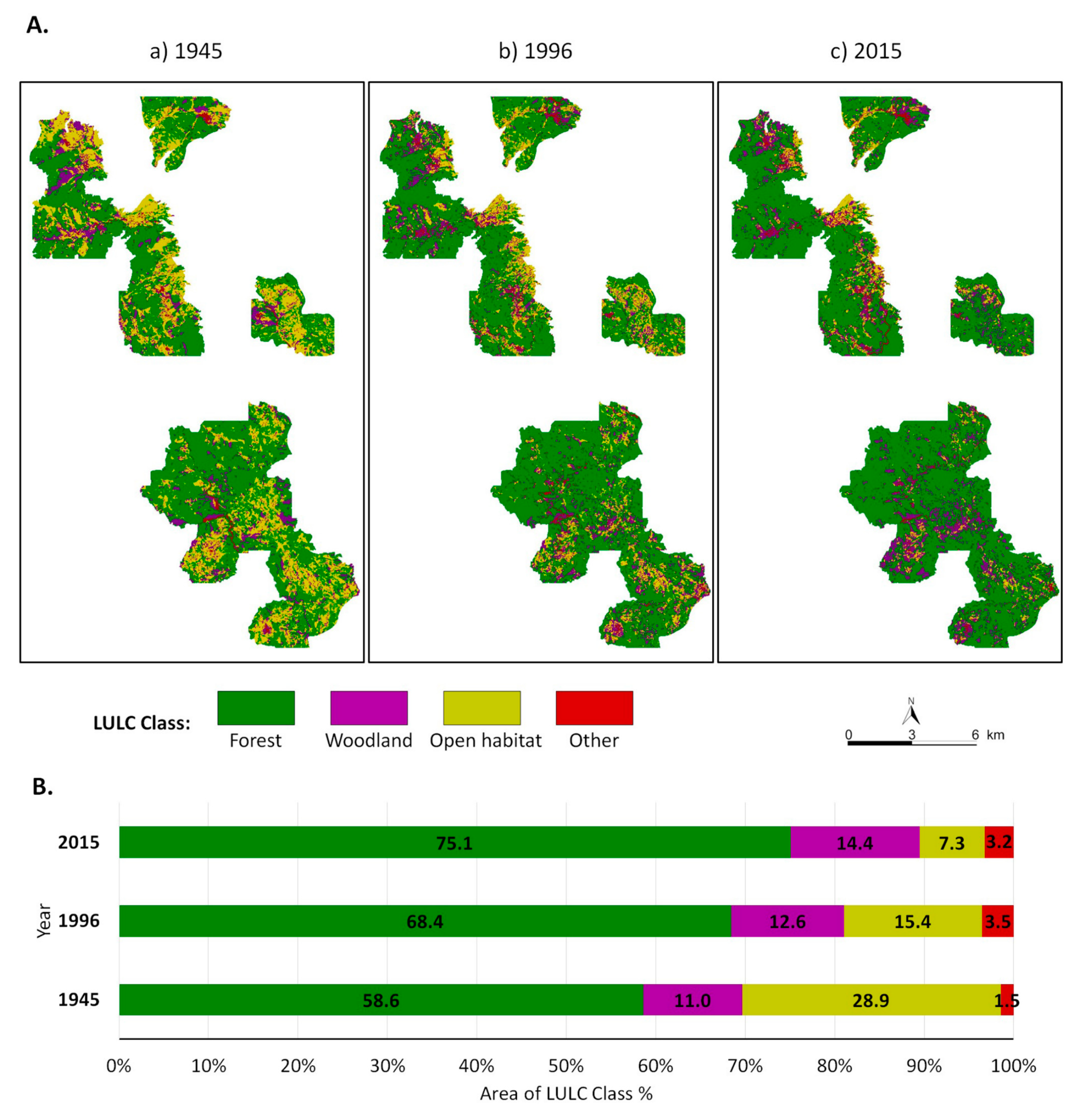
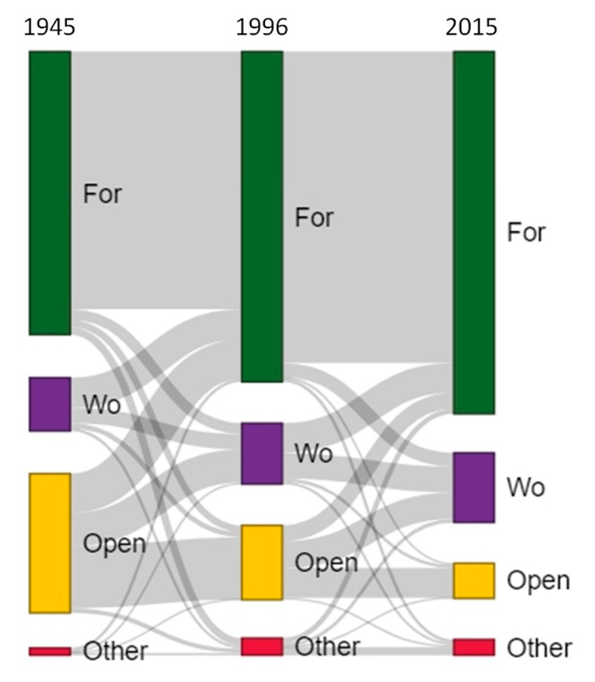
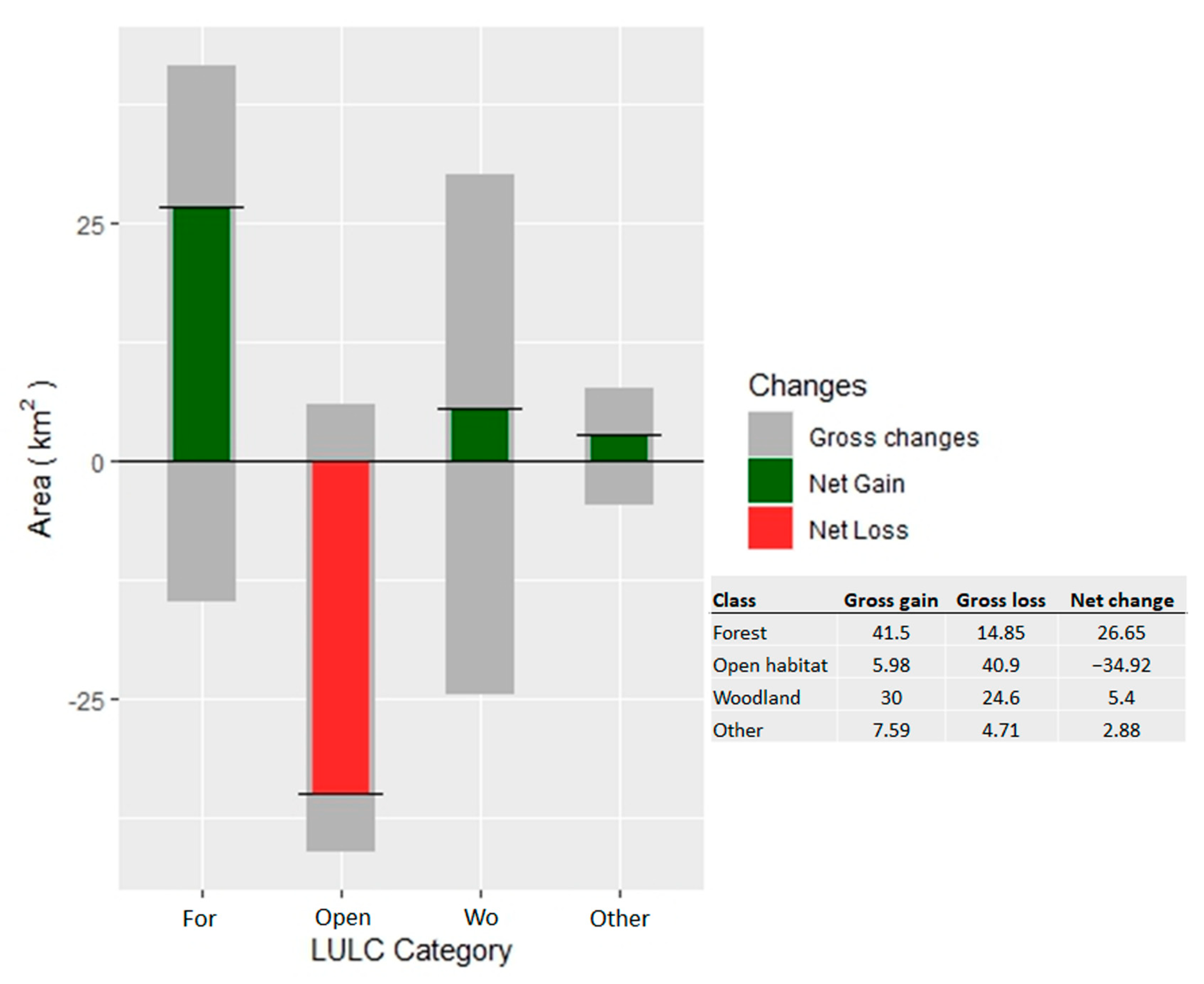
3.1. Land Use/Land Cover Changes

The spatially explicit distribution, along with the percentage cover of the three LULC categories in the study area for the three studied years is presented in Figure 2. The changes of LULC between the studied years were quantified by transition matrices (Figure 2a–c).

There is visual evidence of land abandonment and vegetation succession on the maps of Figure 2. There was a noticeable reduction in the total surface area of open habitats over time. Open habitats being second in area cover with 28.87% in 1945 decreased to 15.42% in 1996 and 7.28% in 2015. We can observe that the forest class dominated the entire study area in all the studied years and there was a clear increase in its cover over time. Particularly, forests covered a bit more than half of the study area in 1945 (58.63%) and they gradually increased to 75.07% cover in 2015. There was also a small increase in woodland surface area from 11.04% in 1945 to 12.62% in 1996 and finally 14.42% in 2015. For the other three classes occupying smaller areas (almost 3% combined), there were minor changes throughout the study period.

For the period 1945–1996, the transition matrix (

Table 2. Transition matrices of LULC classes in the study area (left part of the table) for the periods 1945 to 1996 (A), 1996 to 2015 (B) and 1945 to 2015 (C). Transition matrix values represent the percentage cover of LULC classes. The right part of the table (separated from the left part by a vertical line) presents the area of each land cover class (in hectares and in percentage of total surface of the study area) at the starting and end years of the period, as well as the difference between them (again in hectares and percentage values).

A: 1945–1996	Forest	Woodland	Open Habitat	Other	1945 (ha)	1996 (ha)	Δ (ha)	1945%	1996%	Δ %
Forest	0.91	0.04	0.02	0.03	6589.38	7691.81	1102.44	58.63	68.44	9.81
Woodland	0.57	0.29	0.09	0.05	1241.25	1418.38	177.12	11.04	12.62	1.58
Open habitat	0.28	0.24	0.45	0.03	3244.12	1732.56	−1511.56	28.87	15.42	−13.45
Other	0.41	0.22	0.06	0.31	163.69	395.69	232	1.46	3.52	2.06
B: 1996–2015	Forest	Woodland	Open habitat	Other	1996 (ha)	2015 (ha)	Δ (ha)	1996%	2015%	Δ %
Forest	0.94	0.04	0.01	0.01	7691.81	8437.06	745.25	68.44	75.07	6.63
Woodland	0.49	0.42	0.05	0.04	1418.38	1620.62	202.25	12.62	14.42	1.8
Open habitat	0.22	0.36	0.4	0.03	1732.56	817.62	−914.94	15.42	7.28	−8.14
Other	0.3	0.2	0.04	0.46	395.69	363.12	−32.56	3.52	3.23	−0.29
C: 1945–2015	Forest	Woodland	Open habitat	Other	1945 (ha)	2015 (ha)	Δ (ha)	1945%	2015%	Δ %
Forest	0.93	0.04	0.01	0.02	6589.38	8437.06	1847.69	58.63	75.07	16.44
Woodland	0.67	0.24	0.03	0.05	1241.25	1620.62	379.38	11.04	14.42	3.38
Open habitat	0.43	0.32	0.22	0.04	3244.12	817.62	−2426.5	28.87	7.28	−21.59
Other	0.47	0.19	0.04	0.31	163.69	363.12	199.44	1.46	3.23	1.77

) shows that there was an intense loss of open habitat surface in the study area (−13.45%). Of the 1945 open habitat surface area, 45% remained stable with the biggest loss being transitioned to forest (28%) and woodland (24%). In this period, the second biggest change was afforestation (9.81%). Forest gains were primarily driven by woodlands and open habitats, as 57% of woodlands and 28% of open habitats were converted to forests. Forest was also the class with the smallest surface loss as 91% of its total area remained unchanged.

Almost the same change pattern continued for the period 1996–2015. Open habitat class again showed the greatest loss among all the classes (−8.14%). In this period, 40% of the open habitats remained stable, with 36% turning to woodlands and 22% to forests. The second biggest change was afforestation (6.63%), and forest was the class with the lowest surface loss as 94% of its total area remained unchanged. Forest gains were primarily driven by woodlands and open habitats, as 49% of woodlands and 22% of open habitats were converted to forests.

Overall, for the study period 1945–2015 we observed a great loss of open habitats by 21.59% of the total study area and an expansion of forests by 16.44%, while for woodlands there was a minor expansion of 3.38%. In other words, during the period 1945–2015, the open habitat class lost 74.8% of the area it had in 1945, while the woodland and forest classes increased their areas by 30.56% and 28.04%, respectively, in comparison with the areas they had in 1945. The changes of LULC classes shown in Table 2 and described above are graphically depicted in Figure 3.

Net and gross LULC change analysis (Figure 4) for the overall study period, 1945–2015, revealed that the largest net changes were the decrease in open habitat area (34.92 km²) and the increase in forest area (26.65 km²). However, in these classes there were also significant gross losses of forests (14.85 km²) and minor gross gains of open habitats (5.98 km²). The woodland class had great gross changes within the studied period, with the gross gain being 6-fold higher than net change and gross loss 5-fold higher. The abovementioned gross changes of woodlands resulted, at the end of the studied period, in a relatively small net gain, equal to 5.4 km².

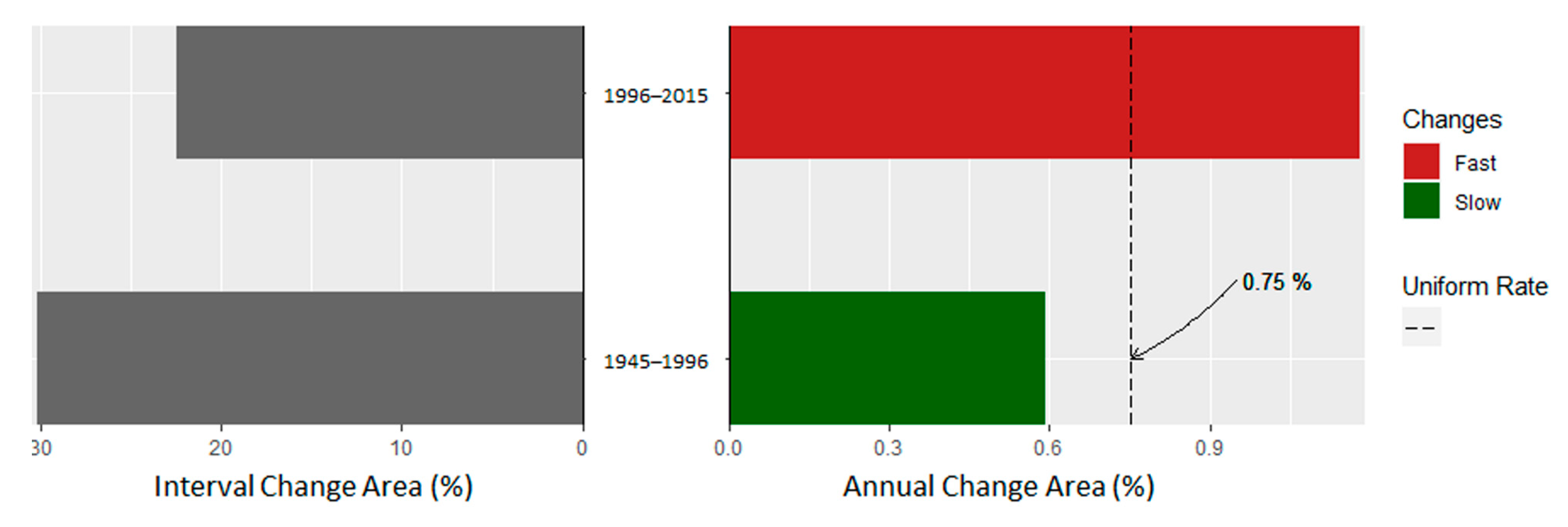
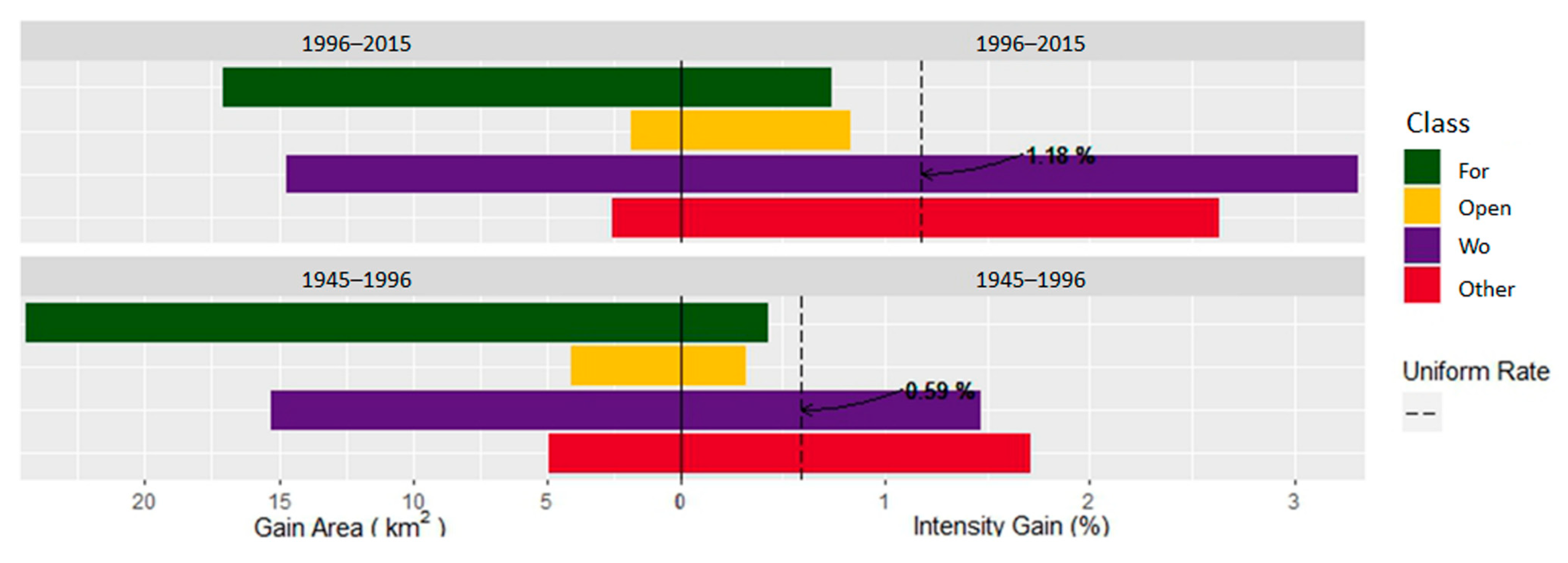
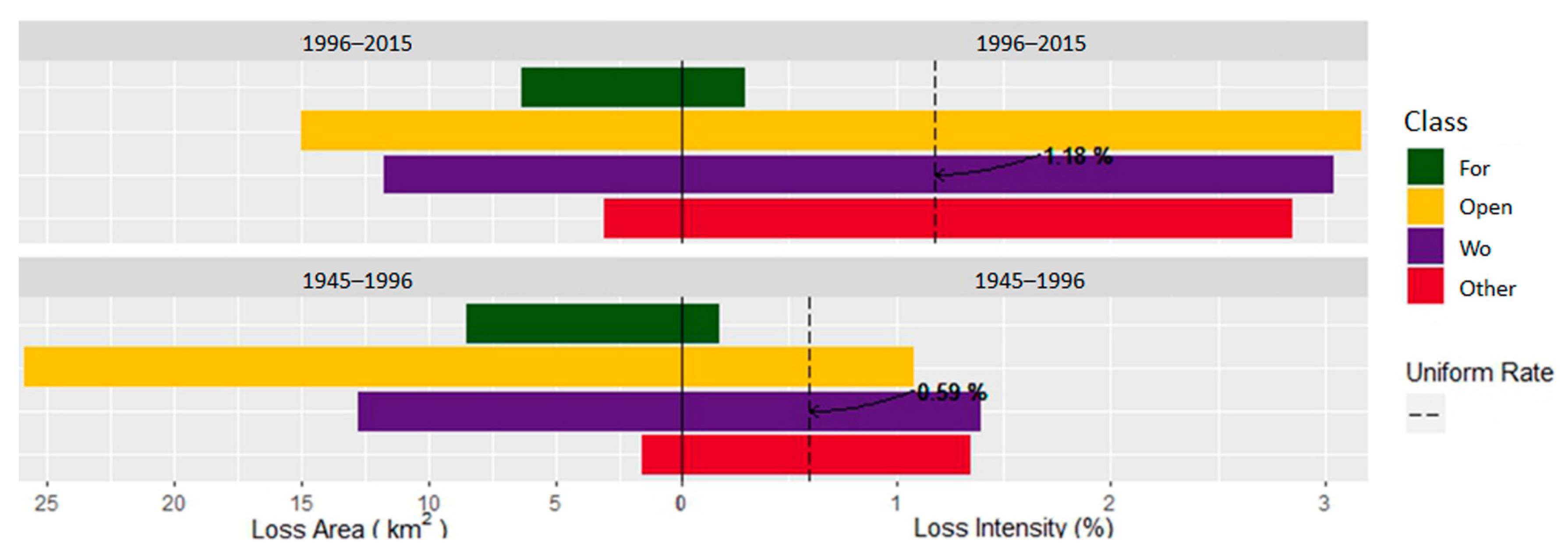
3.2. Intensity Analysis

Changes in the landscape during the first interval (1945–1996) affected a greater extent of the study area than those during the second interval (1996–2015) (Figure 5). However, based on the intensity analysis on the interval level, annual land transformation accelerated significantly in the more recent period (1996–2015) (Figure 5).

Results on the class level of gains revealed that in both studied periods, the forest and woodland had the major gains (Figure 6). During 1945–1996, forests gained 24.4 km² and woodlands 15.3 km² and during 1996–2015 forests gained 17.1 km² and woodlands 14.7 km². Although forests had the biggest observed gain, this had a lower rate than the hypothesized uniform one across the landscape (i.e., it was dormant), for both periods. Open habitat change was also dormant during both periods. On the other hand, for both periods, woodlands were active (had a rate of gain higher than the hypothesized uniform one across the landscape).

Results on the class level of loss reveal that in both studied periods the open habitats and woodlands had the major losses (Figure 7). During 1945–1996, the open habitat class lost 15 km², woodland 11.8 km² and forest 6.33 km². During 1996–2015, the open habitat class lost 25.9 km², woodland 12.8 km² and forest 8.52 km². Open habitat and woodland surface losses were active compared with the hypothesized uniform intensity across the total landscape, but forests were dormant.

In the Supplementary Material (Figures S4–S6), we present the transition level intensity analysis for the LULC classes (except the Others class) with active gains or losses. Furthermore, we present the transition level intensity analysis for forest gain (Figure S7) because this class had the second highest net change in absolute values, albeit it was not found as having an active gain.

Woodland gain is driven mainly by open habitats’ succession to woodlands (Figure S4). This transition was much more intense during the second studied period (1996–2015), but for both periods was found as targeted. There is also a part of forest that changed to woodland, possibly because of disturbances and retrogressive succession, but this transition was not found as higher than the uniform intensity across LULC classes.

Open habitat loss was mainly due to its transition to woodland and this transition was found as targeted for both periods, but more intense for the recent one (Figure S5). In the first period (1945–1996) the area of open habitats that became forests was larger than those that became woodlands, but this relation of the abovementioned transitions was inverted in the recent period. Nevertheless, the transition of open habitats to forests was found as avoided (lower than the uniform intensity across LULC classes).

Woodland loss was almost equally shared among transitions to forests and open habitats for both periods studied (Figure S6). Both types of transitions were marginally higher or lower than the uniform transition among LULC classes, for both studied periods.

Forest gain may be attributed mainly to the succession of woodlands to forests in both periods studied (Figure S7). The intensity of this transition was found as higher than the uniform intensity across LULC classes for both periods but it was accelerated in the recent period.

3.3. Comparison of Land Use/Land Cover Changes and Their Intensity between Municipal Districts with Different Trends of Population Size

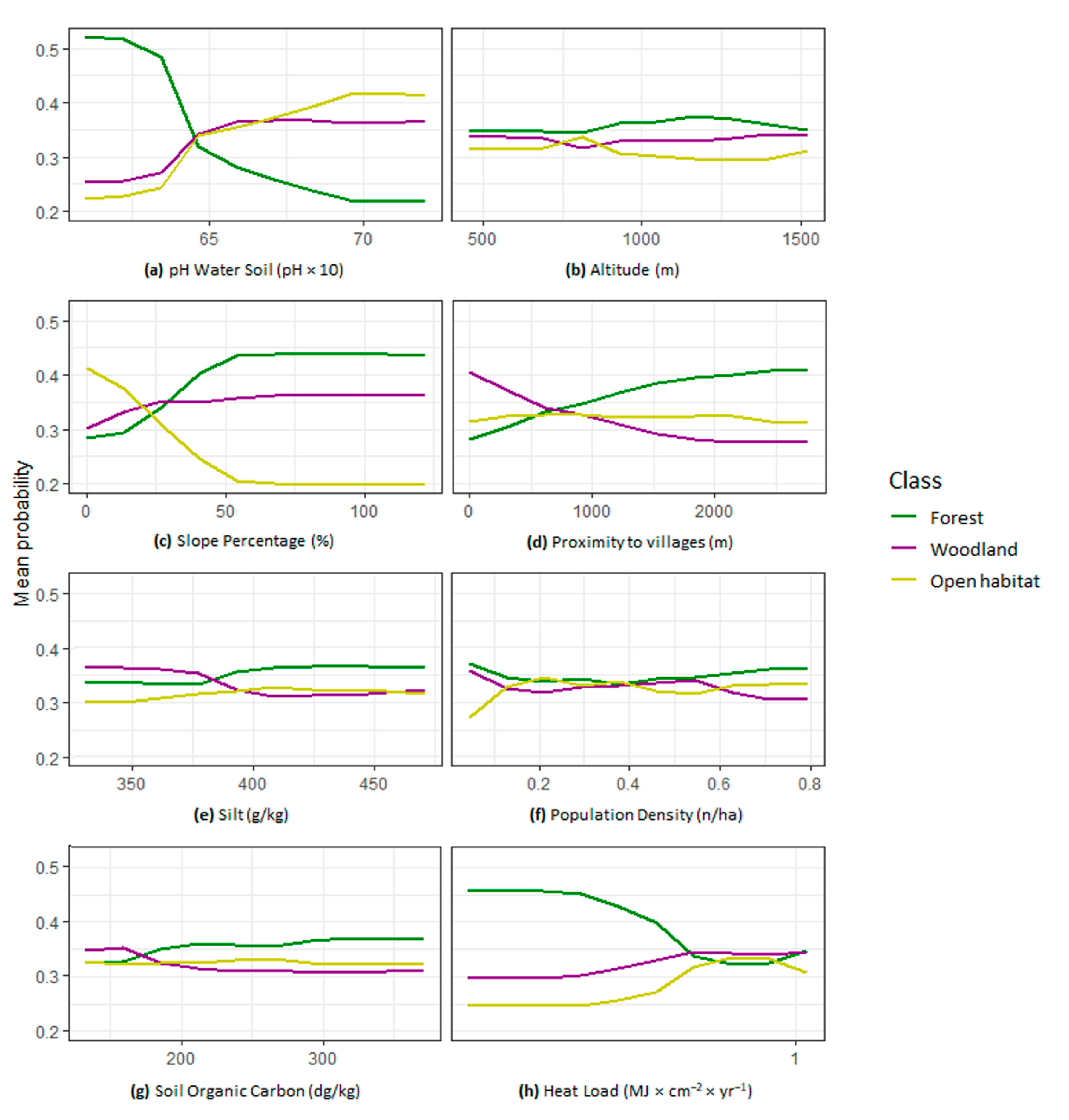
In the Supplementary Material, we present most of the results of the former two sections for the two types of municipal districts that were distinguished based on their different population trends. As was described in the Section 2.1, in the municipal districts close to the lake, the population increased after 1980 or 1990 and in 2011 was approximately of the same size as that at the beginning of the studied period. On the contrary, in the municipal districts away from the lake, population size continued to decrease more or less during the whole studied period and in 2011 was about one-third of that at the beginning of the studied period. In the Supplementary Material, we present the following results for the abovementioned two types of municipal districts (close to lake, far from lake): (a) transition matrices and LULC class cover data for the periods 1945 to 1996, 1996 to 2015 and 1945 to 2015 (Table S2), (b) Sankey diagrams of LULC changes between the studied years (Figure S8), (c) net and gross LULC changes (Figure S9), (d) interval level intensity analysis (Figure S10), (e) LULC class level intensity analysis for area gain (Figure S11) and (f) LULC class level intensity analysis for area loss (Figure S12).

From all the abovementioned tables and figures concerning the two types of municipal districts, it is evident that there were not significant differences between the two types of municipal districts and that the patterns in both of them were similar between each other as well as to the patterns described for the whole study area.

3.4. Random Forest

The RF model exhibited an acceptable land class classification with an accuracy of 0.7 and a Kappa of 0.43. The variables that were found to be most important for the RF modeling were soil acidity, altitude, slope, proximity to villages, silt soil content, population density and carbon soil content. According to the Partial Dependence Plots (PDP) (Figure 8), the probability of occurrence of the three main LULC classes depends strongly on soil pH, with forests being favored at soils with pH values lower than 6.4 and woodlands and open habitats at soils with pH values greater than 6.4 (Figure 8a). The probability of occurrence of forests is weakly positively related to altitude, while that of open habitats negatively (Figure 8b). A slope of up to 50% was found almost linearly related to the probabilities of occurrence of forests and open habitats (positively and negatively, respectively), while above the value of 50%, the probabilities of occurrence of forests and open habitats remained stable to their highest and lowest values, respectively (Figure 8c). Slope also had a positive relation to the probability of occurrence of woodland, albeit much weaker. Proximity to villages was found to positively affect the probability of occurrence of forests and negatively affect that of woodlands, while it had no significant effect on the probability of open habitat occurrence (Figure 8d). Increased soil silt content (<≈380 g/kg) was found to favor forest occurrence against that of woodlands (Figure 8e). Population density seems to have a complex effect on the probabilities of the three main LULC classes. In very small values it favored the occurrence of forests and woodlands and was related to lower probabilities of occurrence of open habitats. In medium values of population density (from about 0.2 to lower than 0.6), no systematic trend regarding the effect on LULC class occurrence was found, while in values higher than about 0.6 it seemed to favor the occurrence of forests against that of woodlands, while leaving unaffected the probability of open habitats (Figure 8f). Soil organic carbon favors the occurrence of forests against that of woodlands (Figure 8g). Finally, slopes receiving less heat load from solar radiation (e.g., slopes of north or northeastern aspect) favor the occurrence of forests against that of woodlands or open habitats. At slopes with high heat loads (e.g., of southwestern aspect), the probabilities of occurrence of all the three LULC classes are more or less equal (Figure 8h).

3.5. Landscape Metrics

The results of the landscape metrics calculated for all the studied years and per LULC class, as well as at the landscape level are presented in

Table 3. Landscape metrics calculated for all the studied years and per LULC class, as well as at the landscape level. NP: Number of patches, LPI: Largest Patch Index, FRAC_AM: Area-Weighted Mean of Fractal Dimension Index, ENN_MN: Mean of Euclidean Nearest Neighbor Distance, IJI: Interspersion Juxtaposition Index.

	NP			LPI			FRAC_AM			ENN_MN			IJI
	1945	1996	2015	1945	1996	2015	1945	1996	2015	1945	1996	2015	1945	1996	2015
Forest	470	414	261	18.2	33.79	37.2	1.33	1.36	1.34	59.73	56.66	56.11	72.01	94.85	85.23
Woodland	2198	2768	2506	0.58	0.29	0.61	1.16	1.17	1.19	70.27	65.35	65.65	76.25	86.31	76.79
Open habitat	1105	1550	1234	3.11	1.24	0.6	1.28	1.23	1.18	69.55	69.28	77.26	67.77	80.11	85.97
Other	666	2675	2326	0.18	0.08	0.12	1.15	1.10	1.11	102.6	76.56	83.21	94.93	88.00	87.96
Landscape	4439	7407	6327	18.25	33.79	37.19	1.29	1.31	1.30	73.82	69.74	73.98	72.82	88.85	84.06

. The number of patches index (NP) at the landscape level significantly increased from 1945 to 1996 and then moderately decreased. NP results followed the same pattern for woodlands and open habitats, but for forests were found declining from 1945 to 2015. The Largest Patch index (LPI) was increasing through time at the landscape level and for forests, which represent the dominant LULC class in all periods. For the open habitat class, LPI had a decreasing trend, while for the woodland class it decreased from 1945 to 1996 and then increased again. The Area-Weighted Mean of Fractal Dimension index (FRAC_AM) at the landscape level increased within the first studied period (1945–1996) and in the next period it received an intermediate value between those it had in 1945 and 1996. This metric followed the same pattern for the forest class as well. For the woodland class, FRAC_AM was found to increase during the whole studied period, while open habitats followed the opposite trend.

The Mean of Euclidean Nearest Neighbor Distance index (ENN_MN) at the landscape level decreased during the first studied period and then increased, reaching its highest value for the year 2015. For the forest and woodland classes, it decreased from 1945 to 1996 and then (in 2015) it remained approximately stable, while for open habitats it remained approximately stable in the years 1945 and 1996 and then increased significantly. The Interspersion Juxtaposition index (IJI) increased during the first studied period and then slightly decreased for the landscape level. It followed a corresponding pattern for the forest and woodland classes, but with a higher decrease in the last studied year (2015), especially for the woodland class. On the contrary, it continued to increase for the whole studied period for open habitats.

Finally, the Simpson’s Diversity index (SIDI) calculated at the landscape level followed a clear decreasing pattern, with values equal to 0.5605, 0.4906 and 0.4093 for the years 1945, 1996 and 2015, respectively.

4. Discussion

4.1. Main Patterns of LULC Changes

The most basic finding of this study concerns the important trends of changes in the landscape of the study area during the 70 years studied (1945–2015). These changes include the significant decrease in open habitat cover and the increase in forest cover. The expansion of forests found by the present study is in agreement with respective results of other studies in mountainous areas of Europe [2,5,12]. Furthermore, the overall reduction of open habitat area by 74.8% in 70 years is of the same magnitude with that found in other regions of northern Greece, such as the 87% decrease in open habitats in northern Pindus [38] and the 93.6% decrease in Rhodope [50].

On the other hand, in regions of southern Greece the reduction of open habitat area was much less prevalent. Specifically, in the Peloponnese (Mt Zireia), a reduction of 20.7% of open habitat area was found [51], and a 19.7% reduction in Aetoloakarnania [52]. In other Mediterranean countries, both large and small decreases of open habitat have been found. For instance, in the Central Spanish Pyrenees, a reduction of open habitat (87.4%) [53] similar to the one found in the present study was observed, but in central Spain [54] and central Apennines [55] the decrease in open habitat cover was much smaller (17.8% and 16%, respectively) and similar to that found in areas of southern Greece.

Such differences in the magnitude of open habitat reduction and of forest increase, respectively, between areas in Greece as well as the Mediterranean region may comprise an interesting research question. These differences may be due to several reasons. In Greece, there is an intuitive observation, made by practitioners of natural environment management during the last two decades, that overgrazing, which was a main topic for vegetation conservation status in Greece until the 1960s or 1970s, has been almost completely ceased in northern and central Greece, but is still affecting many areas in the southern part of the country (including some Aegean islands). Bauer & Bergmeier [56] found grazing to constitute a high pressure throughout the wood pasture areas of western Crete. Thus, it seems that traditional as well as current practices of land use and grazing differ even within the same country. Furthermore, forest cover in Greece is decreasing with decreasing latitude because climate as well as soil conditions are harsher for forest growth in the southern part of the country [57]. Concerning the soil conditions, they are harsher partly due to the more long-term and intense land use in this part of the country. Therefore, on the basis of the abovementioned notes, we may speculate that the differences in the magnitude of land cover changes of open habitats and forests among different parts of Greece are due to differences in the climatic and soil conditions, which may or may not favor the growth and expansion of forests, as well as to differences in land use history, but also current land use practices. Nevertheless, as it was previously mentioned, further research focused on this issue is needed to better understand the different profiles of LULC changes in different areas due to land abandonment.

4.2. Rate of LULC Changes

Intensity analysis results clearly showed that the rate of LULC change accelerated during the recent period. This pattern was steady for all the levels of intensity analysis (interval, class and transition) and for all the cases of gains or losses of LULC classes that were found as active or targeted. Accelerated changes caused by secondary succession after land abandonment were also some of the main findings of a recent study carried out in an area in northern Pindus [38], located about 100 km away from our study area. On the other hand, land abandonment rates in Europe are reported to slow down [5], as the recultivation of formerly unused farmland has become an important trend, especially in Central and Eastern Europe [23]. Furthermore, succession rates following abandonment are expected to decrease over time as vegetation types more vulnerable to succession progressively lose their area and therefore less and less area of them remain to be changed through succession [53]. However, our results do not seem to follow such a pattern. Although in 1996 open habitats covered 15.4% of the study area, in 1945 they covered 28.9%, and the rate of abandonment and subsequent succession was almost doubled within the period 1996–2015 in comparison with that found for the period 1945–1996. This contradiction may be partly due to the progress of the intensity of land abandonment in time, as well as by qualitative characteristics of abandonment. Agricultural activities (farming and livestock raising) actually constitute disturbances made in vegetation that impede ecological succession. In this study, as well as in similar studies, land abandonment is quantified through vegetation cover changes as well as by socioeconomic variables, such as trends in population and livestock numbers. However, some other characteristics of abandonment (qualitative or quantitative) are more difficult to measure or take into account. For instance, the introduction of grazing in abandoned farmland or the existence of grazing from a reduced but still sufficient number of livestock in extended areas can halt ecological succession and conceal the effects of land abandonment for a period of time [58,59,60]. Additionally, according to Sidiropoulou et al. [61], on Mount Vermio, succession in areas where grazing still occurs is less intense relative to those where grazing has been ceased completely.

Vegetation succession is a complex process and its rate and the pathways that it follows are influenced by many factors some of which are of stochastic character [62]. Although vegetation succession may be more or less a directional process [63], its progress is not linear and there are some thresholds (e.g., concerning disturbances intensity) that should be exceeded so as to have compositional and structural changes in vegetation and thus changes of land cover. Succession characteristics may also be differentiated by the land use legacies of the different parts of the landscape, as well as from their post-abandonment treatment [62]. Thus, a different interpretation concerning the expected rate of LULC change in a post-abandonment process may be the acceleration of LULC change rate after a period of time and after the completion of change of a large proportion of certain LULC classes. This interpretation may be explained by the time needed for the alteration of soil conditions after abandonment through the establishment of pioneer species as well as for species migration from nearby vegetation patches. A good indication that in our study area the LULC change is accelerated throughout the studied years is the increase in area of the woodland class, which constitutes the intermediate stage in the directional vegetation succession after land abandonment. We may hypothesize that when the area of this intermediate class starts to decrease (under the condition that the intensity and extend of disturbances will not increase), we could expect to have a deceleration of LULC changes in the study area. Of course, such a deceleration should be expected to happen when a threshold of the proportion of the area of LULC classes representing prodromus vegetation stages have transitioned to forests (the final stage of transition). It seems that in our study area that threshold has not been reached yet.

4.3. Factors Driving Land Abandonment and Consequent Vegetation Succession

Several studies highlight the positive correlation between the depopulation size and the degree of land abandonment [2,10,11,64]. In our case, there was a population decline from 1940 to 1981 in the total study area. The population decrease during this period was the major factor that led to the beginning of the land abandonment process. After 1981, the population started to increase in the study area. Despite this increase, our results show that the resettlement of the area did not succeed to halt land abandonment and vegetation succession. Furthermore, even in the municipal districts around Lake Plastiras in which a population size of 2011 reached the respective levels of 1940, we found similar patterns of LULC changes with those found for the municipal districts away from the lake, although the later had continuous, decreasing population trends, with their population in 2011 corresponding to one-third of their population in 1940.

A possible explanation for this fact may be that the majority of the new residents of the study area are not engaged in agriculture, but in the tourism sector [65]. Thus, the number of people working in primary production (i.e., agricultural activities) continued to decline. This fact constitutes another type of land abandonment, poorly described in Europe before [66]. These results also agree with a study in northern Pindos, where the increase in population caused by the tourism development in Papigo villages did not prevent further agricultural abandonment [67]. Similar findings were also provided by Van Der Sluis et al. [3], who concluded that there is no indication that tourism contributes to slowing down abandonment.

The explanatory variables with higher importance in our model were soil pH, altitude, slope, proximity to villages, soil silt content, population density, soil organic carbon content and heat load. From these factors, soil pH, proximity to villages, soil silt content, soil organic carbon content and heat load determine mainly how favorable the ecological conditions are for the development of forest vegetation and thus vegetation succession progress. Specifically, more acidic soils favor the development of forest vegetation because of their higher soil water capacity. Soils with higher content in silt and organic carbon are richer in resources needed for tree growth. Slopes with lower heat load (e.g., slopes of north or northeastern aspect) have lower evapotranspiration and thus have moister microclimate, which in turn favor tree growth in Mediterranean area [68,69]. Finally, areas far away from villages face lower probabilities of human-induced disturbances and thus have higher probabilities to be forested. The rest of the factors (altitude, slope and population density) mainly affect the possibilities of farmland abandonment. Farmlands at higher altitudes and with higher inclination are usually less productive and thus more prone to abandonment [38,70,71,72,73,74].

4.4. Landscape Patterns Caused by Land Abandonment

Our results regarding the landscape metrics revealed different aspects of the same story. Specifically, they strengthen our overall conclusion that land abandonment and the subsequent vegetation succession have already progressed, and furthermore they have entered their semifinal stage before their completeness. The results concerning landscape metrics that provide the main support to the abovementioned conclusion are the following: (a) the number of patches (NP index) of the early and intermediate succession stages (open habitat, woodland) have already started to decrease in the recent period after their increase during the first period, (b) the largest patch index (LPI) of the intermediate succession stage (woodland), though having a decreasing trend in the first period, changed to an increasing trend in the latter period, (c) patch complexity (FRAC_AM index) of the intermediate succession stage (woodland) continued to increase for the total studied period, while the final stage of succession and dominant LULC class (forest) started to decrease in the last period, (d) the values of class isolation measure (ENN_MN index) were stabilized in the last period for the more final stages of succession (woodland and forest) while having an increasing trend during the latter period for open habitat and (e) the intermixing of classes (IJI index) has already turned to a decreasing trend despite the initial increasing trend.

The overall narrative that the abovementioned findings support is that vegetation has already recovered during the first studied period after the reduction of disturbances caused by agricultural activities, while it subsequently entered a homogenization phase where complexity and mosaicism in the landscape were rapidly reduced and final successional stages of vegetation exclusively dominated the landscape. Similarly to the results of the intensity analysis, the LULC changes have accelerated during the last period, and this is also demonstrated by some landscape metrics such as the LPI and FRAC_AM indices for the woodland class. Furthermore, the landscape metrics showed that the recent period also constitutes the semifinal stage of the land abandonment–vegetation succession process, as some landscape metrics have started to stabilize or decrease in the second period after an initial increase during the first period (e.g., ENN_MN and IJI indices for woodland and forests).

Finally, the Simpson’s Diversity index showed a continuous decline of LULC class diversity, which was even more intense during the recent period, albeit in a much shorter length in comparison with the first period.

Our results concerning the landscape metrics are in agreement with those of other studies for mountainous regions in Europe [75,76,77] and the Mediterranean region [78]. The homogenization of the landscape and the significant shrinkage of open habitats is expected to comprise an important threat factor for many species hosted in such ecosystems [79], a fact that has already been reported in the recent Red List of European habitat types [14]. Mountainous landscapes in Greece and in Mediterranean region turned to be less diverse than they were a few decades ago [79,80], and it seems that they are quickly reaching to a minimization of their diversity.

5. Conclusions

We found a great decrease in the area of open habitats (i.e., grasslands and agriculture land), which at the end of the studied period represented only the one-fourth of the area they had 70 years ago. In the literature, the reduction of open habitat areas of the same magnitude is reported for Greece or the Mediterranean region, but there are also cases in which two- or three-fold lower values of a corresponding reduction were found. We hypothesize that such differences in the proportion of open habitat reduction in the last decades may be due to ecological conditions that favor or not the re-establishment and expansion of forests, as well as to land use history and current practices.

The rate of abandonment and subsequent vegetation succession was almost doubled in the recent period (1996–2015) in comparison with that in the former period (1945–1996). This acceleration, although possibly related to the progress of the intensity of land abandonment over time, could be at least partly explained on the basis of the ecology of vegetation succession. Specifically, some time is needed (e.g., very few to several decades) for the alteration of soil conditions after abandonment through the establishment of pioneer species as well as for species migration from nearby vegetation patches. When these vegetation succession processes advance, the rate of LULC changes should be expected to accelerate.

Our study area included municipal districts with two different types of population trends, giving us the opportunity to explore if there is any difference in LULC change patterns among them. Although the difference of population trends among municipal districts was significant, we found the same LULC changes for all the municipal districts. We attributed this finding to the fact that the increase in population in the municipal districts, which happened in the last decades, was caused by (re-)establishment of inhabitants that are not engaged with the primary sector, while the population of inhabitants working in the primary sector continued to decline in all the municipal districts. Thus, we conclude that repopulation of countryside cannot unconditionally ensure any halting effect on the land abandonment process.

Concerning the factors that have the most important effect on the probability of occurrence of LULC classes through time and space, we concluded that these may be classified into two groups, i.e., those concerning ecological conditions favoring the development and re-establishment of forest vegetation and those that are related to the probabilities of farmland abandonment.

Finally, the landscape patterns revealed by the landscape metrics, but also on the basis of the results of the intensity analysis, led us to the conclusion that land abandonment and the subsequent vegetation succession have already progressed in the study area and entered their semifinal stage before their completeness and the establishment of a more or less absolute dominance of the forest, which represents the final succession stage (provided that intensity of disturbances from agricultural activities or other causes do not increase). Furthermore, land abandonment results in a continuous reduction of LULC class diversity at the landscape level.

References

1. Verburg, P.H.; van Berkel, D.B.; van Doorn, A.M.; van Eupen, M.; van den Heiligenberg, H.A.R.M. Trajectories of Land Use Change in Europe: A Model-Based Exploration of Rural Futures. Landsc. Ecol. 2010, 25, 217–232. [Google Scholar] [CrossRef]
2. MacDonald, D.; Crabtree, J.R.; Wiesinger, G.; Dax, T.; Stamou, N.; Fleury, P.; Gutierrez Lazpita, J.; Gibon, A. Agricultural Abandonment in Mountain Areas of Europe: Environmental Consequences and Policy Response. J. Environ. Manag. 2000, 59, 47–69. [Google Scholar] [CrossRef]
3. van der Sluis, T.; Arts, B.; Kok, K.; Bogers, M.; Busck, A.G.; Sepp, K.; Loupa-Ramos, I.; Pavlis, V.; Geamana, N.; Crouzat, E. Drivers of European Landscape Change: Stakeholders’ Perspectives through Fuzzy Cognitive Mapping. Landsc. Res. 2019, 44, 458–476. [Google Scholar] [CrossRef] [Green Version]
4. García-Ruiz, J.M.; Lasanta, T.; Nadal-Romero, E.; Lana-Renault, N.; Álvarez-Farizo, B. Rewilding and Restoring Cultural Landscapes in Mediterranean Mountains: Opportunities and Challenges. Land Use Policy 2020, 99, 104850. [Google Scholar] [CrossRef]
5. Schuh, B.; Andronic, C.; Derszniak-Noirjean, M.; Gaupp-Berghausen, M.; Hsiung, C.H.; Münch, A. Research for AGRI Committee—The Challenge of Land Abandonment after 2020 and Options for Mitigating Measures; European Parliament, Policy Department for Structural and Cohesion Policies: Brussels, Belgium, 2020. [Google Scholar]
6. Perpiña, C.C.; Kavalov, B.; Ribeiro, B.R.; Diogo, V.; Jacobs, C.; Batista, E.S.F.; Baranzelli, C.; Lavalle, C. Territorial Facts and Trends in the EU Rural Areas within 2015–2030. Available online: https://publications.jrc.ec.europa.eu/repository/handle/JRC114016 (accessed on 18 January 2023).
7. Dax, T.; Schroll, K.; Machold, I.; Derszniak-Noirjean, M.; Schuh, B.; Gaupp-Berghausen, M. Land Abandonment in Mountain Areas of the EU: An Inevitable Side Effect of Farming Modernization and Neglected Threat to Sustainable Land Use. Land 2021, 10, 591. [Google Scholar] [CrossRef]
8. Săvulescu, I.; Mihai, B.-A.; Vîrghileanu, M.; Nistor, C.; Olariu, B. Mountain Arable Land Abandonment (1968–2018) in the Romanian Carpathians: Environmental Conflicts and Sustainability Issues. Sustainability 2019, 11, 6679. [Google Scholar] [CrossRef] [Green Version]
9. Aide, T.M.; Grau, R. ECOLOGY: Enhanced: Globalization, Migration, and Latin American Ecosystems. Science 2004, 305, 1915–1916. [Google Scholar] [CrossRef]
10. Rey Benayas, J.M.; Martins, A.; Nicolau, J.M.; Schulz, J.J. Abandonment of Agricultural Land: An Overview of Drivers and Consequences. CAB Rev. 2007, 2. [Google Scholar] [CrossRef] [Green Version]
11. Cramer, V.A.; Hobbs, R.J.; Standish, R.J. What’s New about Old Fields? Land Abandonment and Ecosystem Assembly. Trends Ecol. Evol. 2008, 23, 104–112. [Google Scholar] [CrossRef]
12. Keenleyside, C.; Tucker, G. Farmland Abandonment in the EU: An Assessment of Trends and Prospects; WWF and IEEP: London, UK, 2010. [Google Scholar]
13. Moreira, F.; Russo, D. Modelling the Impact of Agricultural Abandonment and Wildfires on Vertebrate Diversity in Mediterranean Europe. Landsc. Ecol. 2007, 22, 1461–1476. [Google Scholar] [CrossRef]
14. Janssen, J.; Rodwell, J.; García Criado, M.; Gubbay, S.; Haynes, T.; Nieto, A.; Sanders, N.; Landucci, F.; Loidi, J.; Ssymank, A.; et al. European Red List of Habitats Part 2. Terrestrial and Freshwater Habitats; European Commission: Luxembourg, 2016; ISBN 978-92-79-61588-7. [Google Scholar]
15. Agnoletti, M. Rural Landscape, Nature Conservation and Culture: Some Notes on Research Trends and Management Approaches from a (Southern) European Perspective. Landsc. Urban Plan. 2014, 126, 66–73. [Google Scholar] [CrossRef]
16. Halada, L.; Evans, D.; Romão, C.; Petersen, J.-E. Which Habitats of European Importance Depend on Agricultural Practices? Biodivers. Conserv. 2011, 20, 2365–2378. [Google Scholar] [CrossRef]
17. Prishchepov, A.V.; Radeloff, V.C.; Baumann, M.; Kuemmerle, T.; Müller, D. Effects of Institutional Changes on Land Use: Agricultural Land Abandonment during the Transition from State-Command to Market-Driven Economies in Post-Soviet Eastern Europe. Environ. Res. Lett. 2012, 7, 024021. [Google Scholar] [CrossRef]
18. Fayet, C.M.J.; Reilly, K.H.; Van Ham, C.; Verburg, P.H. What Is the Future of Abandoned Agricultural Lands? A Systematic Review of Alternative Trajectories in Europe. Land Use Policy 2022, 112, 105833. [Google Scholar] [CrossRef]
19. Tasser, E.; Tappeiner, U. Impact of Land Use Changes on Mountain Vegetation. Appl. Veg. Sci. 2002, 5, 173–184. [Google Scholar] [CrossRef]
20. Rey Benayas, J.M.; Galván, I.; Carrascal, L.M. Differential Effects of Vegetation Restoration in Mediterranean Abandoned Cropland by Secondary Succession and Pine Plantations on Bird Assemblages. For. Ecol. Manag. 2010, 260, 87–95. [Google Scholar] [CrossRef] [Green Version]
21. van der Sluis, T.; Sunyer, C.; Capello, J.; Manteiga, L.; Rufino, R. Input document for the 3rd Natura 2000 Seminar for the Mediterranean Biogeographical region. In Proceedings of the Support for the Natura 2000 Biogeographical Process—ENV.D.3/SER/2017/0010, Calabria, Italy, 4–7 May 2021. [Google Scholar]
22. Plieninger, T.; Hui, C.; Gaertner, M.; Huntsinger, L. The Impact of Land Abandonment on Species Richness and Abundance in the Mediterranean Basin: A Meta-Analysis. PLoS ONE 2014, 9, e98355. [Google Scholar] [CrossRef] [Green Version]
23. Estel, S.; Kuemmerle, T.; Alcántara, C.; Levers, C.; Prishchepov, A.; Hostert, P. Mapping Farmland Abandonment and Recultivation across Europe Using MODIS NDVI Time Series. Remote Sens. Environ. 2015, 163, 312–325. [Google Scholar] [CrossRef]
24. Strid, A.; Tan, K. Mountain Flora of Greece; Cambridge University Press: Cambridge, UK, 1986; ISBN 978-0-7486-0207-0. [Google Scholar]
25. Beck, H.E.; Zimmermann, N.E.; McVicar, T.R.; Vergopolan, N.; Berg, A.; Wood, E.F. Present and Future Köppen-Geiger Climate Classification Maps at 1-Km Resolution. Sci. Data 2018, 5, 180214. [Google Scholar] [CrossRef] [Green Version]
26. Karger, D.N.; Conrad, O.; Böhner, J.; Kawohl, T.; Kreft, H.; Soria-Auza, R.W.; Zimmermann, N.E.; Linder, H.P.; Kessler, M. Climatologies at High Resolution for the Earth’s Land Surface Areas. Sci. Data 2017, 4, 170122. [Google Scholar] [CrossRef] [Green Version]
27. Nakos, G. Site Classification, Mapping and Evaluation: Technical Specifications; Institute of Mediterranean Forest Ecosystems and Forest Products Technology, Ministry of Agriculture: Athens, Greece, 1991. [Google Scholar]
28. Bohn, U.; Gollub, G.; Hettwer, C.; Neuhäuslová, Z.; Raus, T.; Schlüter, H.; Weber, H. Karte Der Natürlichen Vegetation Europas/Map of the Natural Vegetation of Europe. Maßstab/Scale 1 : 2 500 000; Landwirtschaftsverlag: Münster, Germany, 2004. [Google Scholar]
29. Rahman, M.; Saha, S. Multi-Resolution Segmentation for Object-Based Classification and Accuracy Assessment of Land Use/Land Cover Classification Using Remotely Sensed Data. J. Indian Soc. Remote Sens. 2008, 36, 189–201. [Google Scholar] [CrossRef]
30. Kosztra, B.; Büttner, G.; Hazeu, G.; Arnold, S. Updated CLC Illustrated Nomenclature Guidelines; European Environment Agency: Wien, Austria, 2017; pp. 1–124. [Google Scholar]
31. OpenDEM. Available online: https://www.opendem.info/opendemeu_download_highres.html (accessed on 18 January 2023).
32. MOLUSCE—QGIS Python Plugins Repository. Available online: https://plugins.qgis.org/plugins/molusce/ (accessed on 19 January 2023).
33. Quan, B.; Pontius, R.G.; Song, H. Intensity Analysis to Communicate Land Change during Three Time Intervals in Two Regions of Quanzhou City, China. GIScience Remote Sens. 2020, 57, 21–36. [Google Scholar] [CrossRef]
34. Aldwaik, S.Z.; Pontius, R.G. Intensity Analysis to Unify Measurements of Size and Stationarity of Land Changes by Interval, Category, and Transition. Landsc. Urban Plan. 2012, 106, 103–114. [Google Scholar] [CrossRef]
35. Gao, C.; Zhou, P.; Jia, P.; Liu, Z.; Wei, L.; Tian, H. Spatial Driving Forces of Dominant Land Use/Land Cover Transformations in the Dongjiang River Watershed, Southern China. Environ. Monit. Assess. 2016, 188, 84. [Google Scholar] [CrossRef]
36. Exavier, R.; Zeilhofer, P. OpenLand: Software for Quantitative Analysis and Visualization of Land Use and Cover Change. R J. 2021, 12, 359–371. [Google Scholar] [CrossRef]
37. Biau, G.; Scornet, E. A Random Forest Guided Tour. Test 2015, 25, 197–227. [Google Scholar] [CrossRef] [Green Version]
38. Kiziridis, D.A.; Mastrogianni, A.; Pleniou, M.; Karadimou, E.; Tsiftsis, S.; Xystrakis, F.; Tsiripidis, I. Acceleration and Relocation of Abandonment in a Mediterranean Mountainous Landscape: Drivers, Consequences, and Management Implications. Land 2022, 11, 406. [Google Scholar] [CrossRef]
39. McCune, B.; Keon, D. Equations for Potential Annual Direct Incident Radiation and Heat Load. J. Veg. Sci. 2002, 13, 603–606. [Google Scholar] [CrossRef]
40. Poggio, L.; de Sousa, L.M.; Batjes, N.H.; Heuvelink, G.B.M.; Kempen, B.; Ribeiro, E.; Rossiter, D. SoilGrids 2.0: Producing Soil Information for the Globe with Quantified Spatial Uncertainty. Soil 2021, 7, 217–240. [Google Scholar] [CrossRef]
41. Main Page ELSTAT—ELSTAT. Available online: https://www.statistics.gr/en/home/ (accessed on 18 January 2023).
42. Ragkos, A.; Koutsou, S.; Karatassiou, M.; Parissi, Z.M. Scenarios of Optimal Organization of Sheep and Goat Transhumance. Reg. Env. Chang. 2020, 20, 13. [Google Scholar] [CrossRef]
43. Probst, P.; Boulesteix, A.-L. To Tune or Not to Tune the Number of Trees in Random Forest? J. Mach. Learn. Res. 2017, 18, 6673–6690. [Google Scholar]
44. Probst, P.; Wright, M.; Boulesteix, A.-L. Hyperparameters and Tuning Strategies for Random Forest. WIREs Data Min. Knowl. Discov. 2019, 9, 6673–6690. [Google Scholar] [CrossRef] [Green Version]
45. Cre Kuhn, M.; Wing, J.; Weston, S.; Williams, A.; Keefer, C.; Engelhardt, A.; Cooper, T.; Mayer, Z.; Kenkel, B.; R Core Team; et al. Caret: Classifi.cation and Regression Training (Version 6.0-90). Available online: https://cran.r-project.org/web/packages/caret/index.html (accessed on 17 October 2022).
46. RStudio Team RStudio: Integrated Development Environment for R (Version 2022.7.2.576 “Spotted Wakerobin”); RStudio PBC: Boston, MA, USA, 2022; Available online: http://www.rstudio.com/ (accessed on 17 October 2022).
47. Goldstein, A.; Kapelner, A.; Bleich, J.; Pitkin, E. Peeking Inside the Black Box: Visualizing Statistical Learning with Plots of Individual Conditional Expectation. J. Comput. Graph. Stat. 2015, 24, 44–65. [Google Scholar] [CrossRef] [Green Version]
48. Greenwell, B.M. Pdp: An R Package for Constructing Partial Dependence Plots. R J. 2017, 9, 421–436. [Google Scholar] [CrossRef] [Green Version]
49. McGarigal, K.; Marks, B.J. Spatial Pattern Analysis Program for Quantifying Landscape Structure; Gen. Tech. Rep. PNW-GTR-351; US Department of Agriculture, Forest Service, Pacific Northwest Research Station: Corvallis, OR, USA, 1995; Volume 351, pp. 1–122.
50. Oikonomakis, N.; Ganatsas, P. Land Cover Changes and Forest Succession Trends in a Site of Natura 2000 Network (Elatia Forest), in Northern Greece. For. Ecol. Manag. 2012, 285, 153–163. [Google Scholar] [CrossRef]
51. Chouvardas, D.; Karatassiou, M.; Stergiou, A.; Chrysanthopoulou, G. Identifying the Spatiotemporal Transitions and Future Development of a Grazed Mediterranean Landscape of South Greece. Land 2022, 11, 2141. [Google Scholar] [CrossRef]
52. Xystrakis, F.; Psarras, T.; Koutsias, N. A Process-Based Land Use/Land Cover Change Assessment on a Mountainous Area of Greece during 1945–2009: Signs of Socio-Economic Drivers. Sci. Total Environ. 2017, 587–588, 360–370. [Google Scholar] [CrossRef]
53. Pueyo, Y.; Beguería, S. Modelling the Rate of Secondary Succession after Farmland Abandonment in a Mediterranean Mountain Area. Landsc. Urban Plan. 2007, 83, 245–254. [Google Scholar] [CrossRef] [Green Version]
54. Arnaez, J.; Lasanta, T.; Errea, M.P.; Ortigosa, L. Land Abandonment, Landscape Evolution, and Soil Erosion in a Spanish Mediterranean Mountain Region: The Case of Camero Viejo. Land Degrad. Dev. 2011, 22, 537–550. [Google Scholar] [CrossRef]
55. Malavasi, M.; Carranza, M.L.; Moravec, D.; Cutini, M. Reforestation Dynamics after Land Abandonment: A Trajectory Analysis in Mediterranean Mountain Landscapes. Reg. Env. Chang. 2018, 18, 2459–2469. [Google Scholar] [CrossRef]
56. Bauer, E.-M.; Bergmeier, E. The Mountain Woodlands of Western Crete—Plant Communities, Forest Goods, Grazing Impact and Conservation. Phytocoenologia 2011, 41, 73–115. [Google Scholar] [CrossRef]
57. Ministry of Agriculture First National Inventory of Greece. General Secretariat of Forests and Natural Environment, Independent Edition; Ministry of Agriculture First National Inventory of Greece: Athens, Greece, 1992. [Google Scholar]
58. Peña-Angulo, D.; Khorchani, M.; Errea, P.; Lasanta, T.; Martínez-Arnáiz, M.; Nadal-Romero, E. Factors Explaining the Diversity of Land Cover in Abandoned Fields in a Mediterranean Mountain Area. CATENA 2019, 181, 104064. [Google Scholar] [CrossRef]
59. Giourga, H.; Margaris, N.S.; Vokou, D. Effects of Grazing Pressure on Succession Process and Productivity of Old Fields on Mediterranean Islands. Environ. Manag. 1998, 22, 589–596. [Google Scholar] [CrossRef]
60. Collins, S.L.; Knapp, A.K.; Briggs, J.M.; Blair, J.M.; Steinauer, E.M. Modulation of Diversity by Grazing and Mowing in Native Tallgrass Prairie. Science 1998, 280, 745–747. [Google Scholar] [CrossRef] [PubMed]
61. Sidiropoulou, A.; Karatassiou, M.; Galidaki, G.; Sklavou, P. Landscape Pattern Changes in Response to Transhumance Abandonment on Mountain Vermio (North Greece). Sustainability 2015, 7, 15652–15673. [Google Scholar] [CrossRef] [Green Version]
62. Pickett, S.T.A.; Cadenasso, M.L.; Meiners, S.J. Vegetation Dynamics. In Vegetation Ecology; John Wiley & Sons, Ltd.: Oxford, UK, 2013; pp. 107–140. ISBN 978-1-118-45259-2. [Google Scholar]
63. Odum, E.P. The Strategy of Ecosystem Development. Science 1969, 164, 262–270. [Google Scholar] [CrossRef] [PubMed] [Green Version]
64. Hatfield, R.; Davies, J. Global Review of the Economics of Pastoralism; IUCN: Nairobi, Kenya, 2006. [Google Scholar]
65. Koutsouris, A. The Battlefield for (Sustainable) Rural Development: The Case of Lake Plastiras, Central Greece. Sociol. Rural. 2008, 48, 240–256. [Google Scholar] [CrossRef]
66. Bilewicz, A.; Bukraba-Rylska, I. Deagrarianization in the Making: The Decline of Family Farming in Central Poland, Its Roots and Social Consequences. J. Rural Stud. 2021, 88, 368–376. [Google Scholar] [CrossRef]
67. Zomeni, M.; Tzanopoulos, J.; Pantis, J.D. Historical Analysis of Landscape Change Using Remote Sensing Techniques: An Explanatory Tool for Agricultural Transformation in Greek Rural Areas. Landsc. Urban Plan. 2008, 86, 38–46. [Google Scholar] [CrossRef]
68. Żywiec, M.; Muter, E.; Zielonka, T.; Delibes, M.; Calvo, G.; Fedriani, J. Long-Term Effect of Temperature and Precipitation on Radial Growth in a Threatened Thermo-Mediterranean Tree Population. Trees 2017, 31, 491–501. [Google Scholar] [CrossRef] [Green Version]
69. Forner, A.; Valladares, F.; Bonal, D.; Granier, A.; Grossiord, C.; Aranda, I. Extreme Droughts Affecting Mediterranean Tree Species’ Growth and Water-Use Efficiency: The Importance of Timing. Tree Physiol. 2018, 38, 1127–1137. [Google Scholar] [CrossRef] [Green Version]
70. Foster, D.R. Land-Use History (1730–1990) and Vegetation Dynamics in Central New England, USA. J. Ecol. 1992, 80, 753–771. [Google Scholar] [CrossRef]
71. Foster, D.R.; Fluet, M.; Boose, E.R. Human or Natural Disturbance: Landscape-Scale Dynamics of the Tropical Forests of Puerto Rico. Ecol. Appl. 1999, 9, 555–572. [Google Scholar] [CrossRef]
72. Flinn, K.M.; Vellend, M.; Marks, P.L. Environmental Causes and Consequences of Forest Clearance and Agricultural Abandonment in Central New York, USA. J. Biogeogr. 2005, 32, 439–452. [Google Scholar] [CrossRef]
73. Gellrich, M.; Zimmermann, N.E. Investigating the Regional-Scale Pattern of Agricultural Land Abandonment in the Swiss Mountains: A Spatial Statistical Modelling Approach. Landsc. Urban Plan. 2007, 79, 65–76. [Google Scholar] [CrossRef]
74. Mallinis, G.; Emmanoloudis, D.; Giannakopoulos, V.; Maris, F.; Koutsias, N. Mapping and Interpreting Historical Land Cover/Land Use Changes in a Natura 2000 Site Using Earth Observational Data: The Case of Nestos Delta, Greece. Appl. Geogr. 2011, 31, 312–320. [Google Scholar] [CrossRef]
75. Jongman, R.H.G. Homogenisation and Fragmentation of the European Landscape: Ecological Consequences and Solutions. Landsc. Urban Plan. 2002, 58, 211–221. [Google Scholar] [CrossRef]
76. Bielsa, I.; Pons, X.; Bunce, B. Agricultural Abandonment in the North Eastern Iberian Peninsula: The Use of Basic Landscape Metrics to Support Planning. J. Environ. Plan. Manag. 2005, 48, 85–102. [Google Scholar] [CrossRef]
77. Geri, F.; Amici, V.; Rocchini, D. Human Activity Impact on the Heterogeneity of a Mediterranean Landscape. Appl. Geogr. 2010, 30, 370–379. [Google Scholar] [CrossRef]
78. Sitzia, T.; Semenzato, P.; Trentanovi, G. Natural Reforestation Is Changing Spatial Patterns of Rural Mountain and Hill Landscapes: A Global Overview. For. Ecol. Manag. 2010, 259, 1354–1362. [Google Scholar] [CrossRef]
79. Jiménez-Olivencia, Y.; Ibáñez-Jiménez, Á.; Porcel-Rodríguez, L.; Zimmerer, K. Land Use Change Dynamics in Euro-Mediterranean Mountain Regions: Driving Forces and Consequences for the Landscape. Land Use Policy 2021, 109, 105721. [Google Scholar] [CrossRef]
80. Chouvardas, D.; Karatassiou, M.; Tsioras, P.; Tsividis, I.; Palaiochorinos, S. Spatiotemporal Changes (1945–2020) in a Grazed Landscape of Northern Greece, in Relation to Socioeconomic Changes. Land 2022, 11, 1987. [Google Scholar] [CrossRef]
Figure 1. Map of the study area (black line) and the 13 municipal districts overlapping with the study area (white line). Municipal districts are given in the map with numbers, while their names are given in the map’s legend. The geographical location of the study area is indicated by a red box in the inserted map of Greece.
Land 12 00846 g001
Figure 2. Land use/land cover (LULC) maps produced for the study area (A), where a: LULC map for the year 1945, b: for the year 1996 and c: for the year 2015, and (B) the percentage of each land cover class for each studied year.
Land 12 00846 g002
Figure 3. Sankey diagram highlighting the main patterns of LULC changes between the studied years (1945, 1996 and 2015). For: Forest, Wo: Woodland, Open: Open habitat, Other: urban, water and rock land cover classes.
Land 12 00846 g003
Figure 4. Net and gross LULC changes in km2 for the overall study period (1945–2015). For: Forest, Wo: Woodland, Open: Open habitat, Other: urban, water and rock land cover classes.
Land 12 00846 g004
Figure 5. Interval level intensity analysis in the study area for the periods 1945–1996 and 1996–2015, for the total change area in each period (left plot) and the rate of change for each period (right plot). The vertical, dashed line at the right plot represents the hypothesized uniform intensity for the total period (1945–2015) and the periods with a bar extending beyond this line are considered as changing fast (red color), while those with a bar before that line are considered as changing slow (green color).
Land 12 00846 g005
Figure 6. LULC class level intensity analysis for area gain in the study area for the 1945–1996 and 1996–2015 periods. Bars that extend to the left of zero axis show the gross surface gain for each LULC class. Bars that extend to the right of zero axis show the intensity of gain for each class. The vertical, dashed line at the right part of the plot depicts the hypothesized uniform intensity across the total landscape of the study area. Classes with bars extending beyond this line are considered as having active gains, while those with bars before that line are considered as having dormant gains. For: Forest, Open: Open habitat, Wo: Woodland, Other: urban, water and rock land cover classes.
Land 12 00846 g006
Figure 7. LULC class level intensity analysis for area loss in the study area for the periods 1945–1996 and 1996–2015. Bars that extend to the left of zero axis show the gross surface loss for each LULC class. Bars that extend to the right of zero axis show the intensity of loss for each class. For the explanation of the vertical, dashed line and the LULC classes, see Figure 6.
Land 12 00846 g007
Figure 8. Partial Dependence Plots (PDP) showing the mean marginal effect of the explanatory variables with the highest importance in the RF model.
Land 12 00846 g008