Article

A GIS-Based Kinematic Analysis for Jointed Rock Slope Stability: An Application to Himalayan Slopes

by
Jagadish Kundu
1,*,
Kripamoy Sarkar
2,
Ebrahim Ghaderpour
1,3,*,
Gabriele Scarascia Mugnozza
1,3 and
Paolo Mazzanti
1,3
1
Department of Earth Sciences & CERI Research Centre, Sapienza University of Rome, P.le Aldo Moro, 5, 00185 Rome, Italy
2
Department of Applied Geology, Indian Institute of Technology (ISM) Dhanbad, Dhanbad 826004, India
3
NHAZCA s.r.l., Via Vittorio Bachelet, 12, 00185 Rome, Italy
*
Authors to whom correspondence should be addressed.
Land 2023, 12(2), 402; https://doi.org/10.3390/land12020402
Submission received: 23 December 2022 / Revised: 20 January 2023 / Accepted: 31 January 2023 / Published: 2 February 2023

Abstract

:
GIS-based kinematic stability analysis in rock slopes is a rare practice in geological engineering despite its immense potential to delineate unstable zones in a mountainous region. In this article, we have used a GIS-based modified technique to assess the efficiency of kinematic analysis in predicting shallow landslides in the rock slopes of the Himalayan mountains on a regional scale. The limited use of this technique is primarily due to the complexities involved in its practical application. To make this technique more effective and convenient usability, we present modified methods and a new application, ‘GISMR’, that works with the aid of GIS software for the determination of kinematic susceptibility. A modified kinematic analysis method was implemented to define the stability in terms of failure susceptibility on a scale of 0 to 100 rather than a conservative result, such as failure or non-failure. We also present another functionality of the GISMR that provides optimised slope angles over a region. This functionality could aid the decision-making process when selecting a suitable location for a road path or other engineering constructions that are impacted by unstable mountain slopes. The applicability of this new method was demonstrated in a rock failure-prone region in the mountains of the Indian Himalayas. The outcomes delineate the unstable slopes in the region, which are intersected by a strategic National Highway 05 and have a long history of landslide-related hazards. It was found that 9.61% of the area is susceptible to failure. However, 2.28% is classified as a low susceptible region, and 2.58% of the area is very-low susceptible. The regions with moderately high, high, and very-high susceptibility cover 2.78%, 1.49%, and 0.46% of the whole area, respectively. The results were evaluated by receiver operating characteristic curve and a frequency ratio method to represent the association between kinematic susceptibility and the mass movement inventory in the area. It is concluded that kinematic susceptibility has a strong relationship with landslide activity in the rock slopes of the Himalayan region.

1. Introduction

Mass movements such as rockfall and rockslides are major hazards in mountainous terrain, mostly along road cuts across jointed rock mass. For an unstable slope undergoing surficial movement or only internal deformation, loose rock blocks likely are released along weak geostructural features [1]. Rock slope morphologies are generally controlled by penetrative discontinuities such as beddings and are modified continuously by mode(s) of failure depending on the arrangement of discontinuities with respect to the slope [2]. The control of structurally weak surfaces to drive deep-seated as well as shallow rock slope instabilities is a well-known phenomenon as proposed by researchers [3,4,5]. In [6], it is shown that geostructural control is dominant in conditioning deep-seated deformation onset in rock slopes. Gupta et al. [7] revealed the predisposition of landslides in the cataclinal slopes of a Himalayan terrain, suggesting the dominance of structural control on the stability of mountain slopes. Some researchers also state that the occurrence of rockslides is highly probable in dip and over-dip slopes [8].
Therefore, knowledge of an area’s structural setting is imperative to predict the rock block release zone, runout distance, associated risk, and counter-remedial measures. However, identifying and localising the release area is highly challenging, especially in a large hilly region. The dislodgement of rock blocks occurs mainly due to unfavourable geometrical arrangements of discontinuities with respect to the slope orientation. In site-specific jointed rock slopes, it is a common practice to analyse discontinuity-driven failures using simple methods such as kinematic analysis and slope mass rating [9,10,11,12] or complex numerical solutions [13,14,15,16]. Simple stability assessment practices such as kinematic analysis consider a single orientation of a slope face and are not suitable for slopes with continuously varying surface morphology, particularly for curved slopes. In addition, the standard (manual) practices are tedious and highly time-consuming, especially for the calculation on a regional scale. Over the last two decades, advanced computerised spatial analysis using geographical information systems (GIS) has enabled the analysis of rock slope failure on a regional scale. The analyses on a regional scale are primarily intended to provide a preliminary and fast indication of an area with possibilities of critical events [17]. For example, Romstad et al. have implemented a GIS approach to assess rockfall-induced tsunami hazards for Norwegian lakes and reservoirs [18]. However, the results may not be adequate for its simplistic assumption of the release area only by a local slope angle threshold and non-consideration of discontinuities responsible for block detachment.
With the advent of computerised techniques, it is possible to incorporate discontinuities into a GIS architecture for further analysis. Using GIS, spatial analysis of rock slopes over a large region is more straightforward when the discontinuities are parallel and regularly spaced with considerable continuity. Thanks to the nature of discontinuities, which occur systematically. This systematic nature of the discontinuities enables us to develop efficient and widely applicable procedures to quantify their weakening effect on mountain slopes. Terzaghi quotes Bruno Sander as “it is certainly easier to imagine random, that is, isotropic jointing for the purpose of computation than it is to find an example of it in nature” [19]. Again, the wide availability of digital elevation models (DEM) has enabled us to solve a variety of mass movement problems using computerised techniques.
Quantitative estimation of the contribution of discontinuities to slope failure on a regional and local scale is critical for assessing slope stability, landslide hazard, risk, and geomorphic evolution. Meentemeyer and Moody [20] pioneered an automatic digital technique for the computation of topographic and bedding angle intersection (TOBIA) to generate a continuous index over a region and classify it categorically into different types such as cataclinal, orthoclinal, and anaclinal slopes. To date, for analysis of geostructural control on rock slope instabilities, TOBIA is most often used by numerous authors probably due to its ease of use in a GIS platform and availability of open-source code [21,22]. However, TOBIA considers only the bedding planes and cannot establish the interaction effect of other discontinuity sets with the bedding and slope morphology. On the other hand, kinematic analysis is a simple and efficient means of quantifying the effect of mutual interaction between all discontinuities and slope surfaces on a hill slope. Despite its enhanced capabilities in predicting structural instabilities, GIS-based kinematic analysis is a rare practice in slope stability assessment due to the absence of publicly available codes and easily implementable procedures. There is a need for a simple methodology and easily implementable algorithm for the widespread use of kinematic analysis to utilise its immense capabilities in regional slope stability analysis and morphological studies. A brief description of the previous methods, techniques, and tools used for GIS-based kinematic analysis is presented in Table A1.
The article is organised as follows. The main contributions of this study are listed in Section 1.1. The state-of-the-art of kinematic analysis and susceptibility analysis are reviewed in Section 1.2 and Section 1.3, respectively. Section 2 describes the materials and methods. The results and discussion are presented in Section 3 and Section 4, respectively. The conclusions and final remarks are presented in Section 5.

1.1. Aim and Contributions

The main aim of this research article was to evaluate the efficiency of rock slope kinematic analysis in predicting shallow landslides in the Himalayan mountains on a regional scale with the help of a modified GIS-based technique. The main contributions of this work are as follows:
(1)
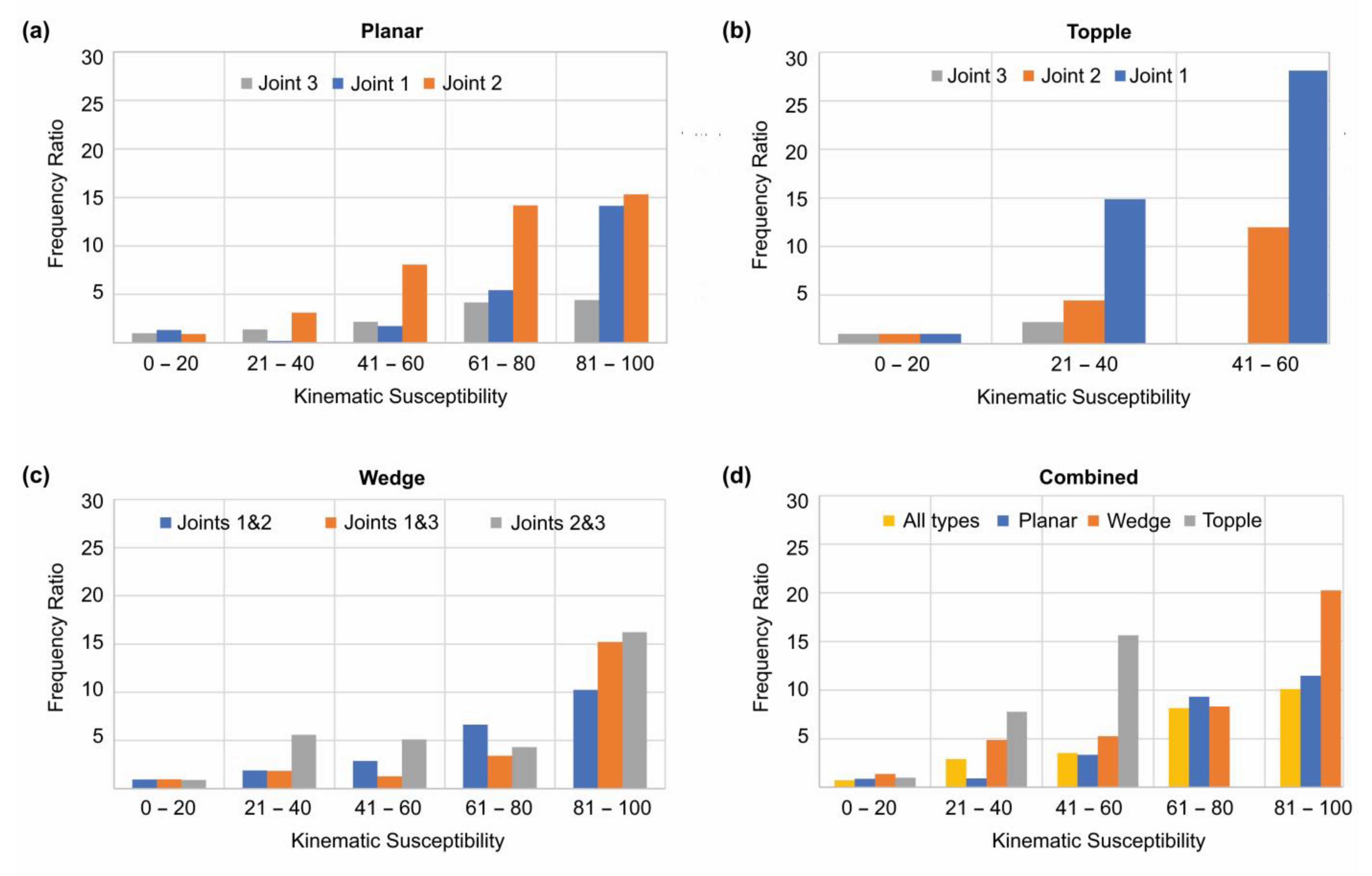
A modified kinematic analysis method is proposed to represent kinematic susceptibility based on the geometrical degree of vulnerability of a failure element, i.e., a plane or intersection within a range from 0 to 100. The modified method is more flexible than the conventional outcomes of zero or one (i.e., fail or no fail).
(2)
An easily implementable algorithm is proposed to perform deterministic rock slope stability analysis. The efficiency of this analysis in predicting rock block release zones is demonstrated through a case study in the mountainous regions of the Indian Himalayas. Subsequently, the results are evaluated by quantifying the association among predicted unstable zones and the inventory of released zones.
(3)
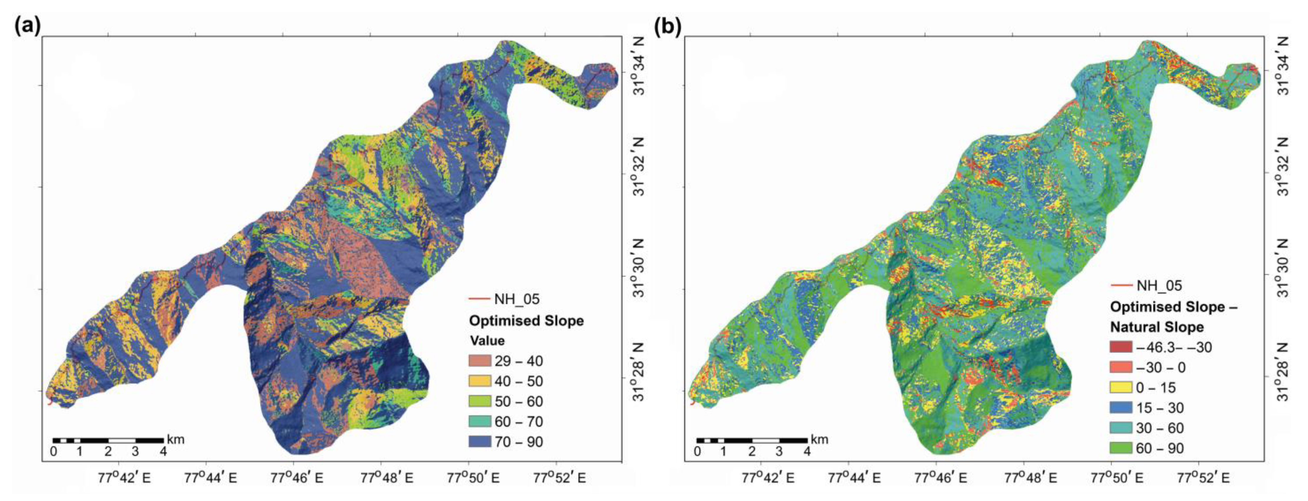
The capability of a slope optimisation algorithm is demonstrated to produce a layer indicating safe and unsafe slopes, which would immensely help preliminary engineering decisions on a large mountainous region.

1.2. State-of-the-Art

Kinematic analysis is commonly performed by the ‘Markland’s test’ to determine the possibility of planar, wedge, and topple failure modes in rock slopes [10]. It is traditionally performed by interpreting projections of joints and slope orientations on a stereonet [23,24,25,26,27,28,29]. The feasibility of a particular type of failure (i.e., planar, wedge, or topple) at a particular morphological setup is determined by the orientation of discontinuity planes, their interaction with each other, and the slope face of the topography. Figure 1 demonstrates the angular relations of discontinuity planes with the planar slope surface along with the notations used afterward. According to Markland, a planar discontinuity in a rock slope is susceptible to failure when the strike of a joint plane is parallel or sub-parallel to the strike of the slope face ( α p     20 ° ) and θ     β P     Φ , i.e., the joint daylights on the slope face and friction angle of the joint plane is less than the dip of the discontinuity. Here, Φ is the joint friction angle, and θ is the inclination of the slope. These notations for θ and Φ are used henceforward. A wedge can be formed with the intersection of two non-parallel discontinuity surfaces. If the plunge of the line of intersection is ± 90 ° in the slope direction (i.e., α w     90 ° ) and θ     β w   Φ (see Figure 1), there is a higher possibility that the wedge will fail. A topple failure may occur along a steeply inwards dipping joint whose strike is nearly parallel to the slope face ( α T     10 ° ). An interlayer sliding between the rock columns may occur if 90 β T + Φ < θ , paving the possibility for flexural topple.
The kinematic analysis based on the projection method is suitable for a site-specific slope with uniform slope angle and slope direction along with uniform distribution and orientation of discontinuities. Furthermore, the manual method of analysis is time-consuming and tedious. With the advent of better computer technology, there are several commercial and open-source software sources that have evolved for stereonet-based kinematic analysis. Available commercial software includes ROCKPACK III (from RockWare), DIPS (from Rocscience), and freely available applications include DIPANALYST (www.dipanalyst.com, accessed on 10 January 2023) for quantitative kinematic analysis and EasySMR (www.jkundu.com/easysmr, accessed on 10 January 2023) based on the modified kinematic analysis [30,31]. A modified stereographic method for wedge analysis and a tool for toppling failure are proposed in [32,33], respectively. In recent years, probabilistic kinematic analysis is widely performed using the stereonet method to include the effect of natural variability in joint orientations [34,35,36,37,38,39,40]. There are few attempts to use discontinuities derived from laser scanning and unmanned aerial vehicle (UAV) point clouds in structural stability analysis [41].
Discontinuity analysis on a computer requires the representation of the planar and linear features as 3D vectors. In [42], a vector model was proposed to calculate angular relationships among mutual interactions between planar features and perform the kinematic analysis; see Equations (1)–(6). These equations are used for the development of GISMR.
If the strike and dip of a discontinuity are α and β , respectively, then the vector normal to the discontinuity ( n ) is given by
n = cos α sin β i + sin α sin β j + cos β k
where i ,   j , and k are conventionally considered unit vectors along x ,   y , and z axes. In the case of a wedge, the plunge ( P ) of the line of intersection is given by,
P = sin 1 T 3 T 1 2 + T 2 2 + T 3 2
Azimuth ( A ) of the line of intersection is given by,
A = tan 1 T 1 T 2
where
T 1 = cos β 1 sin α 2 sin β 2 sin α 1 sin β 1 cos β 2
T 2 = cos β 1 cos α 2 sin β 2 cos α 1 sin β 1 cos β 2
T 3 = sin α 1 sin β 1 sin β 2 cos α 2 cos α 1 sin β 1 sin α 2 sin β 2
For slopes with varying morphology, irregular discontinuity distribution and non-uniform spatial occurrence, analysis on a GIS platform could accomplish a reasonable solution. Following substantial improvement in the application of GIS in geology and geomorphology in the 1990s [43,44,45,46,47,48], several researchers have attempted to include discontinuity analysis in a GIS environment. Meentemeyer and Moody [20] were probably the first to provide a feasible methodology for quantification of the relationship between bedding and surface morphology and classifying the slopes on a GIS platform. They proposed a TOBIA index which uses four parameters (slope, aspect, bedding dip, and azimuth), to estimate topographic/bedding plane intersection angles over large areas to produce a continuous index ranging from 1 to + 1 . This method is widely used for the availability of its computer codes, ease of implementation, and easy disposal of required geologic information. Since TOBIA does not consider other discontinuities that are obvious in the rock mass, the results are not robust to rock fall detection.
Later Gunther (2003) developed a suite of QBASIC programs named SLOPEMAP, which can perform kinematic analysis considering various joint sets [49]. The suite was designed for use with common grid-based computer applications such as ArcView with the “Spatial Analyst” extension, consisting of programs such as DIRCOS, EDGEMAP, ANGMAP, WEDGEFAIL, and STRESSMAP. Though some of the components of SLOPEMAP, such as ANGMAP and WEDGEFAIL, are available as extensions at open-source SAGA GIS, other components of the suite are missing, making it difficult to use. Gunther (2004) came up with rock slope stability GIS (RSS-GIS) as several extension modules for ArcView GIS, software of ESRI (Environmental Systems Research Institute, Inc., Redlands, CA, USA), for the rapid automated mapping of geometrical and kinematical slope properties [50]. Ghosh et al. (2010) have used this suite for rock slope assessment of rock slopes in a large region of Darjeeling Himalaya, India [51,52]. Unfortunately, RSS-GIS is not sold or supported anymore by ESRI, hence making it difficult for public availability. Ji et al. discussed in detail the possible impacts of degrading yield acceleration in Newmark computing frameworks for seismic slope stability analysis [53].
Regional rock slope stability analysis is difficult without adequate information on the spatial distribution of discontinuity orientations at a higher density. The denser the geostructural information per unit area, the better the analysis results that can be obtained. The spatial availability of joint information is usually poor in the geological record due to the inaccessibility of areas in mountainous regions and the high cost of data collection. To the rescue are several techniques developed to determine discontinuity orientations on a regional scale by utilising remotely sensed images in combination with GIS techniques. A semi-automatic GIS model was proposed in [54] for extraction of the orientation of planar structural elements through spaceborne thematic images and the Digital Terrain Model (DTM). In [25], a method was developed for the detection and quantification of a general trend of bedding planes using stereoscopic aerial photographs and the subsequent use of TOBIA to evaluate the dependence of landslide types on local structural settings. There are instances of assessing the rock slope susceptibility utilising laser scanning or UAV point clouds [55,56,57]. A few algorithms have recently been developed to perform three-dimensional kinematic analysis on point clouds [58,59].

1.3. Kinematic Susceptibility

It is well known that the maximum principal stress ( σ 1 ) acts nearly parallel to a mountain slope surface [60]. Therefore, a joint plane or intersection line, which shows more parallelism with the slope surface, has a higher chance of failure due to shear release. In other words, a joint or intersection inclined at a higher angle is generally more susceptible to triggering factors, provided it is on the slope’s surface. The conventional kinematic criteria alone cannot estimate the intensity/degree of the failure potential; therefore, a different method is needed to quantify the degree of vulnerability of a failure element. The existing quantitative methods are often based on the number of discontinuities, which undergo Markland’s test to give results of either zero or one [30,36,37,38,61]. The susceptibility estimation in these methods is based on the manipulation of the number of zeros or ones obtained out of numerous failure elements. However, these types of quantitative estimation are important as they provide practical solutions to include the effect of variability in discontinuity orientation. In our view, the presence of a few unfavourably positioned discontinuities, if penetrative, can give rise to massive failures. Therefore, the assignment of the susceptibility value should be based on the magnitude of unfavourability of a single element rather than the number of discontinuities that satisfies Markland’s test. We have adopted the unfavourability criteria of slope mass rating (SMR) to implement this concept on the mountain slope stability analysis. The adjustment factors of SMR have proven their potential in estimating the probability of unfavourable discontinuity arrangements since its introduction [62]. The rock mass classification system is used worldwide with promising results and is endorsed for effective rock slope stability determination by numerous researchers [31,63,64]. The modification of kinematic analysis to represent the susceptibility of discontinuity arrangement in the range of 0 to 100 is more justified, as it gives a quantitative impression of the failure potential.
SMR is a widely accepted and effective rock mass classification system used as an extension of the Rock Mass Rating system [65] and specifically designed for the stability assessment of rock slopes [62,66]. SMR classification is well known amongst engineering geologists and rock engineering practitioners. The correction factors, namely, F 1 ,     F 2 ,   F 3 , and F 4 , related to mutual slope-discontinuities orientations, are the most advantageous features in SMR. Continuous functions were used in [67] for the quantitative determination of the initially proposed semi-quantitative adjustment factors F 1 ,     F 2 , and F 3 , widely used in SMR calculations. The definitions of F 1 , F 2 , and F 3 are presented in Equations (7)–(10). The table containing the semi-quantitative adjustment factors proposed in [62,66] is represented in [31].
F 1 = 16 25 3 500 tan 1 1 10 α 17    
F 2 = 9 16 + 1 195 tan 1 17 100 β 5
      F 3 = 30 + 1 3 tan 1 γ             or
F 3 = 13 1 7 tan 1 γ 120
where F 1 represents planar, topple and wedge failure, F 2 is planar, topple and wedge failure, F 3 in Equation (9) is planar and wedge failure, and F 3 in Equation (10) is topple failure. The value of F 1 × F 2 × F 3 varies from 0 to 60 and represents an indicator for instability induced by orientation of the failure element (i.e., plane or wedge). The continuous functions of the SMR adjustment factors are used in this modified method to determine the kinematic susceptibility of the failure elements as Equation (11).
  Susceptibility   % = F 1 × F 2 × F 3 60   × 100    
The maximum value of F 1 × F 2 × F 3 can be 60 for a very highly susceptible joint. Hence, the value of F 1 × F 2 × F 3 for the considered failure type is divided by 60 and multiplied by 100 to represent the susceptibility in percentage.
The correction factor F 4 , described in Table 1 in [31], varies from 8 to + 15 depending on the excavation method of the slope: poor blasting ( 8 ), normal blasting or mechanical excavation ( 0 ), smooth blasting ( + 8 ), pre-splitting ( + 10 ), and natural slope ( + 15 ). However, since F 4 is related to damage characteristics of the slope and essential for slope mass rating calculation, we did not consider it for kinematic analysis.

2. Materials and Methods
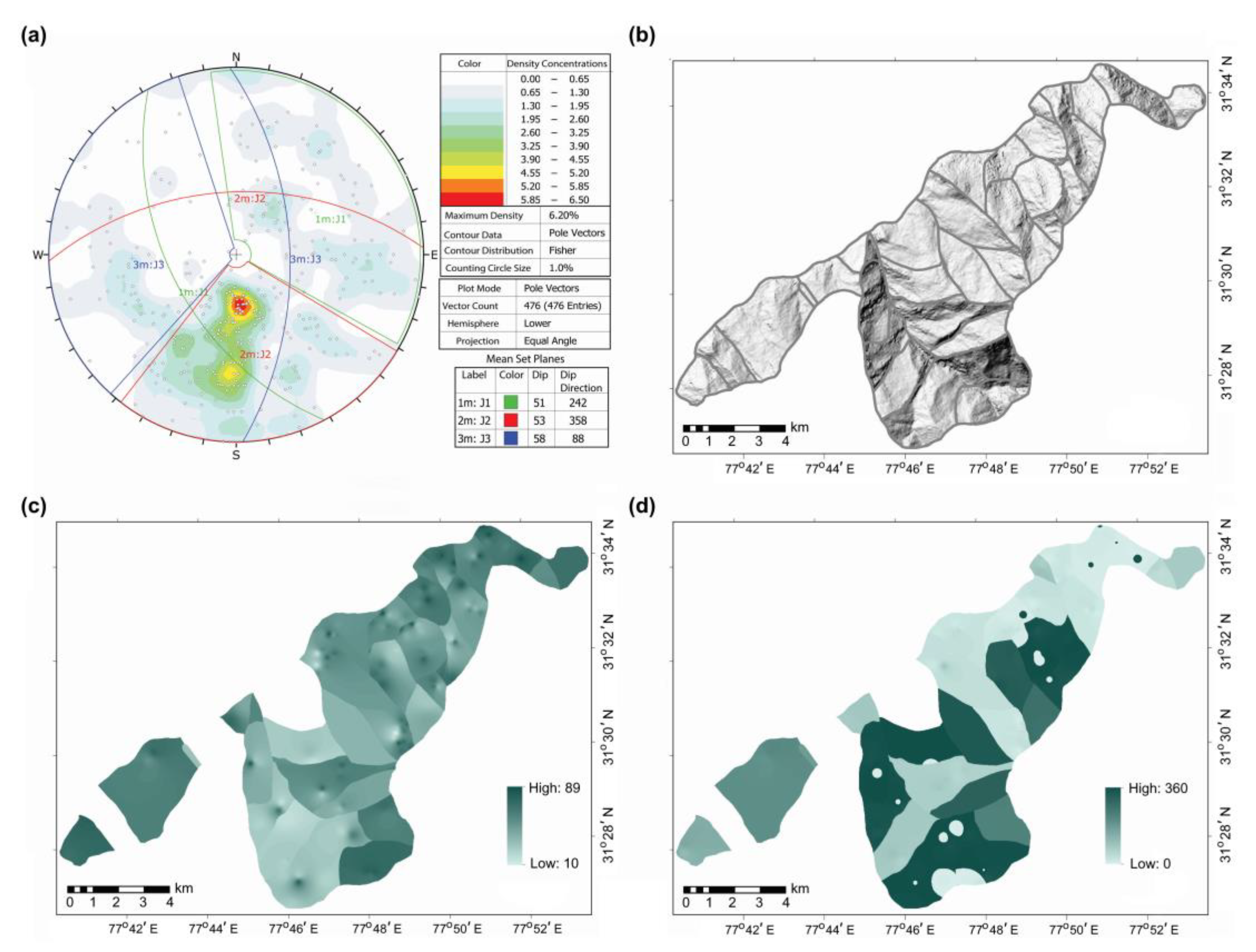
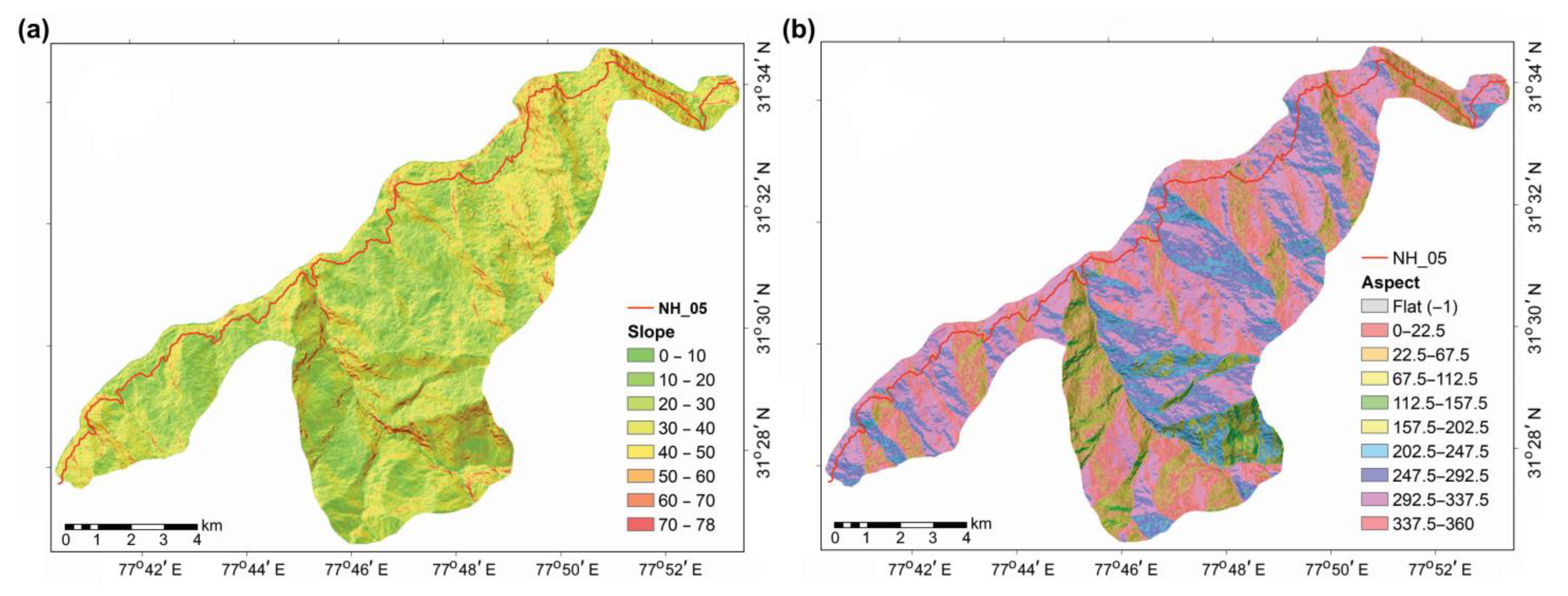
2.1. Study Area

The study area for evaluating modified kinematic susceptibility analysis was chosen to be a highly landslide-prone zone of the Himalayas, partly situated in the district Shimla and partly in the Kinnaur of Himachal Pradesh, India. The analysed rocky terrain covers an area of 102 km2 and possesses various geostructural defects like joints, faults, and thrusts. The Himalayas, being a classic example of a continent–continent collision, comprises two distinct tectogens separated by the Main Central Thrust (MCT). These are the lesser Himalayan tectogen and Tethys Himalaya or higher Himalaya tectogen, with distinct geological histories. The area is situated in the lesser and higher Himalayas region and consists of rocks from the Jutogh formations [68]. This Jutogh nappe tectonically overlies the autochthonous Rampur Group and Wangtu Gneissic Complex [69]. The Jutogh formation is allochthonous to parautochthonous, which has slid over the Jutogh thrust onto the Rampur series [70]. The Jutogh group of rocks has undergone tectonic detachment through ductile shearing [71]. Singh (1979) named this ductile shear detachment the ‘Jeori dislocation’ [68]. The area lies in the Larji–Rampur–Wangtu window zone of the Larji tectonostratigraphic domain [72]. In [21], a part of the Larji–Kullu window was studied, and it was shown that rock detachments accounted for 62% of the total landslide events between 1984 and 2015, among which rockfall, planar rockslide, and rock topple accounted respectively for 30%, 22%, and 10% of the total landslides. The higher percentage of landslides associated with rock failure indicates the dominance of structures as a controlling factor of mass movement in this Himalayan geo-morpho-tectonic setting. A National Highway (NH-05), which runs through the study area on the left bank of river Sutlej, has witnessed significant rock and debris slides in the past and is susceptible to various mass movements at present. Geologically, the area contains various rock types such as quartzites, schists, gneisses, and amphibolite. Detailed lithology and structures of the area collected through field observation and literature are illustrated in the geological map (Figure 2) [68,69,70,73].

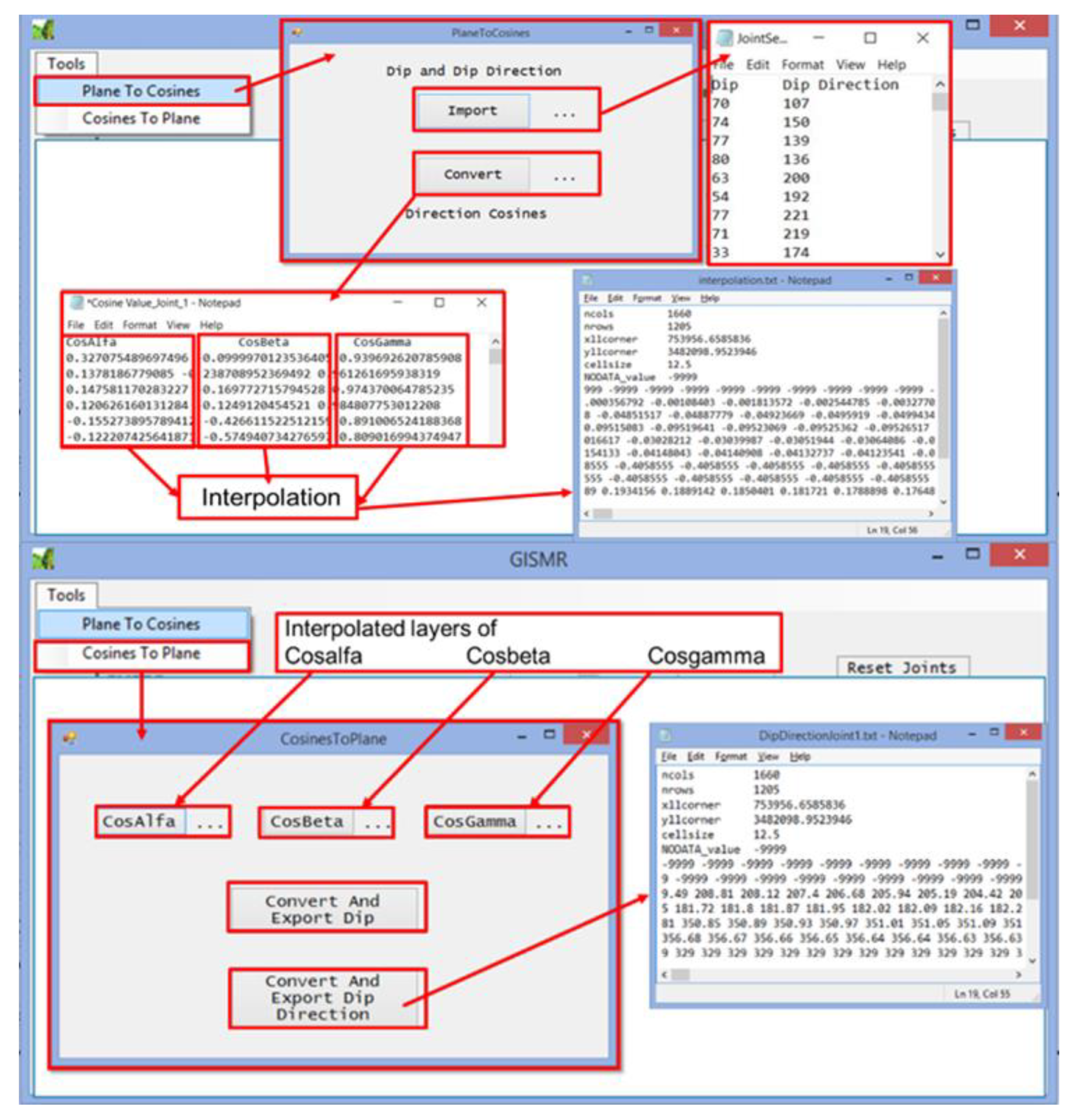
2.2. A Brief Description of GISMR

The computer application GISMR is programmed to perform calculations on a cell-by-cell basis for the kinematic susceptibility and SMR analysis. The program is written using C# on the visual studio Integrated Development Environment. GISMR takes inputs in ASCII/.txt formats, such as the slope, aspect, interpolated continuous dip and dip direction of each discontinuity sets, and friction angle, over a region to perform and produce results for kinematic susceptibility analysis. The program needs an ASCII/.txt file of the RMR value for calculating the Slope Mass Rating. After calculation, the program provides the outputs for kinematic or SMR results (as opted by the user) in .txt files. The calculation and evaluation of SMR using GISMR are chosen not to be included in this article to keep it concise and exclusive for kinematic analysis. Outputs from this application can be imported to GIS platforms such as QGIS or ArcGIS in raster format and visualised for presentation and further analysis purposes. In GISMR, there are options to produce results for planar and topple kinematic/SMR in separate layers for each of the joint sets and n n 1 number of layers ( n is the number of joint sets) for wedge analysis; there is one result layer for each possible intersection between different joint sets. The program has additional functions to produce a single susceptibility layer for each failure mode or for all failure modes. In this case, each pixel contains results of the maximum susceptibility value out of all considered result layers. Another useful algorithm in GISMR is “slope optimisation” which allows for the computation of optimum slope angle according to the user’s input of a susceptibility value that is considered safe for the analysed region. The optimum slope angle in this context means the maximum slope angle at a location that would not give rise to any kinematic failure. This function is especially programmed to aid the preliminary decision-making process for safe engineering construction in a mountainous region that involves threat from surficial failure or excavation, such as roads, dams, and buildings. A screenshot of the GISMR graphical user interface (GUI) showing all the input options and function buttons designed in the application is given in Figure 3, and the algorithm of the program is depicted in Figure 4.

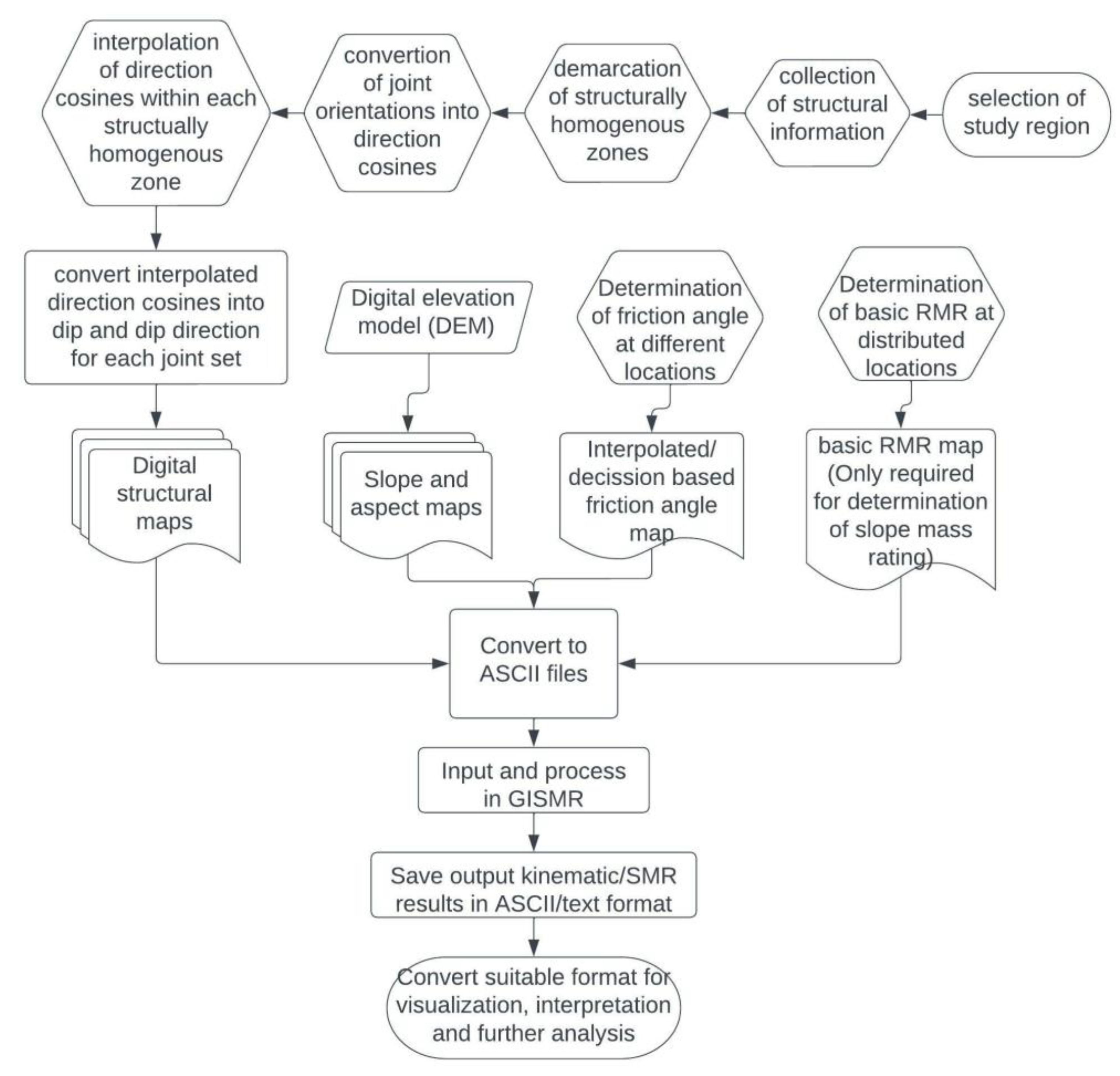
2.3. Methods for Preparation of Input Data

Kinematic stability assessment requires topographic information such as slope, aspect, and discontinuity orientation. To perform the calculations on a GIS platform, we need continuous information about slope, aspect, dip, and dip direction of discontinuities in a grid format. Topographic information can be easily derived from DEM, but there are challenges in preparing continuous gridded information of the dip and azimuth of discontinuities, i.e., a Digital Structural Model (DSM) [51]. For this purpose, we have implemented a procedure in which 3D orientation is converted into vector information using the tools built into GISMR. The conversion of orientations to vector information makes it feasible to work in 2D grid-based GIS applications. The entire algorithm of GISMR is based on a cell-by-cell calculation method using the information in gridded text format. The text files can be exported from the generated or derived raster files of slope, aspect, dip, and dip direction layer. Construction of DSM requires interpolation of the point orientation data collected through field survey or photogrammetric interpretation. Ideally, the zone(s) desired for interpolation should be geo-structurally homogenous, i.e., a sudden change in discontinuity orientation caused by fault, fold, lithological contact, or any other reason should not be expected inside the zone. Below, we describe the steps used to construct the DSM over the studied region successfully. The overall workflow of the analysis using GISMR is illustrated in Figure 5.

2.3.1. Preparation of Geo-Structural Information

It is realised that manual collection of dense discontinuity information in the mountainous region is not always feasible due to the prevalence of inaccessible areas in a higher proportion. In these cases, particular photogrammetric techniques could be used to obtain geo-structural information as suggested by some researchers [54,74,75,76]. However, for the application and validation of the present methodology and algorithms, an area was chosen where sufficiently dense discontinuity orientation and geo-structural boundaries are available in the literature. The authors have also collected joint data along the National Highway 05 that intersects the study region. Proper methods and precautions were followed during the collection of discontinuity data for engineering applications [77]. Discontinuities are symbolically represented in geological maps where the dip amount is represented as a number (text), but the azimuth is represented as an oriented straight line. A Python script was written and implemented on the GIS platform to extract accurate orientations. A total of 357 discontinuities distributed over the regions were obtained from various pieces of literature [68,69,70,73]. Additionally, a stretch of approximately 35 km of National Highway 05, which runs through the selected area, was investigated to obtain 119 discontinuities’ orientations at various locations, making it a total of 476 in the whole region.

2.3.2. Defining Homogenous Structural Domains

The area under consideration is tectonically quite disturbed and contains various geo-structures such as folds, faults, and thrusts (see Figure 2). The discontinuities obtained from the field survey and geological maps in the literature were plotted on to a stereonet in Figure 6a. It can be observed from this figure that the discontinuities are not tightly clustered in the whole region. Consequently, there is a difference in density and distribution of discontinuity orientations within the study area. Spatially distributed discontinuity orientation data, i.e., dip and azimuth, need to be interpolated so that GIS implementation of kinematic feasibility can be carried out over the region. General interpolation over the large region would produce an erroneous and unacceptable DSM. The best possible accuracy of the results from the geological variability can be achieved by dividing the area into smaller segments of structural entities that are considerably homogenous and tightly clustered. In the whole area of 102 km2, several smaller zones are constructed by demarcating possible boundaries that would produce zones of structural homogeneity. The zones were designed in such a way that major structural defects such as faults and thrusts are the permanent boundaries of the zones. In addition, fold axis, major morphological breaks and sharp lithological contacts were considered as a basis for the division of the area into smaller zones. Point orientation data of discontinuities in the area were plotted on Google Earth map and further interpreted to check for any abrupt differences in discontinuity orientations to define area bubbles of possible structural inhomogeneity. Stereographic projections of the discontinuities at each zone were conducted and analysed for tightness of the clusters. Then, the joint orientations of every zone were compared with all instant neighbouring zones and the boundaries were readjusted. However, zone boundaries conforming to major structural defects were not disturbed. The final zones prepared for this study are represented in Figure 6b.

2.3.3. Categorising Joints into Different Sets

The joints in each zone were plotted on a stereonet and differentiated into different joint sets based on orientation similarity. An azimuth difference of 35 ° was set to detect a particular joint set inside each zone. Though most of the joint sets have a maximum azimuth difference of 25 ° , very few numbers of joints, showing a variation of 40 ° , were also included in the set. We detected a maximum of three sets of joints in all of the smaller zones. Few zones have only a single set of joints. Some of the discontinuities in the smaller zones, which exhibited very different orientations from the general trend, were assumed to represent localised distortions and were excluded from creation of DSM.

2.3.4. Interpolation of Discontinuities

Interpolation of joint orientation is not as simple as other distributed observations. Direct interpolation of dip and dip direction values may give errors while crossing Cartesian quadrant boundaries. For example, 350 ° and 10 ° with simple conventional interpolation would result in its arithmetic mean, i.e., 180 ° , while it should be 360 ° or 0 ° . For this purpose, De Kemp (1998) proposed a method to use direction cosines instead of dip and azimuth to interpolate the planar and linear features [47]. For angles in degrees, three direction cosines of the angles α ,   β ,   γ , which are defined as three shortest angles between the unit vector each of the orthogonal Cartesian co-ordinate axes X ,   Y ,   Z , are expressed as:
cos α = cos dip / 57.2958 sin azimuth / 57.2958
cos β = cos ( dip / 57.2958 ) cos azimuth / 57.2958
cos γ = sin dip / 57.2958
where azimuth is the dip direction of a planar feature and the trend of a linear element.
To ease the conversion process, a function was integrated into GISMR. The orientation data can be imported through an ASCII file, as shown in Figure 7 (top), to the ‘plane to cosines’ tool in GISMR, which can then be converted to direction cosines, as indicated in Figure 7 (bottom). Individual direction cosines can be interpolated on a GIS software such as ArcMap or QGIS. The tool ‘Cosines to plane’ can again be used to convert the interpolated grid text data to derive dip and dip direction in an ASCII file. The ASCII file can then be converted into a raster through GIS software to visualise the DSM. The pixel values must not go beyond the input data range for interpolating direction cosines. The value of cos α and cos β must be in the range of 1 to + 1 , and the value of cos γ must lie in the range of 0 to 1 . The IDW interpolation was applied for this study to produce a continuous raster of direction cosines. The zone boundaries were set as barriers to the interpolation process so that the values are interpolated only within the smaller zones of geostructural homogeneity. Examples of interpolated dip and dip direction maps of joint 1 are shown in Figure 6c,d, respectively.

2.3.5. Topographic, Rock Mass Rating and Friction Information

Slope and aspect information for the study area was derived from a 12.5 m resolution ALOS PALSAR DEM using QGIS functions and is shown in Figure 8a,b, respectively. The slope values range from 0 ° to 78 ° , and the aspect value ranges in all directions from 0 ° to 360 ° , covering all ranges in North, East, South and West. The pixel value 1 represents the flat area. The angles of friction for different rocks were determined through the tilt test method at various locations in the area, and a mean friction angle of 26 ° was consideration for the analysis. Several friction angles were collected through the tilt test method at different locations along the National Highway running through the mountainous region. There were also a few locations far away from the highway for which friction angles were determined. We observed a significant variation in the friction angle even in the same lithology (probably due to different roughness patterns) and with no distinct range between different lithologies. Moreover, our dataset was not uniformly collected throughout the region due to inaccessibility in the high, uneven, and treacherous mountains. Thus, we considered the mean value of the friction angle. A raster with a uniform pixel value of 26 ° was generated as an input layer.

2.3.6. Input and Computation in GISMR

As mentioned in the above section, the input raster layers need to be exported into ASCII values using GIS software such as QGIS or ArcGIS before operating on GISMR. For discontinuities, a dip layer and a dip direction layer have to be prepared to represent the orientation of a single set of joints. Hence, a total of six layers (e.g., for joint 1 in Figure 6c,d) were prepared for three joint sets in the analysed area. The RMR layer, which is optional, needs to be prepared for a region of interest if the user needs to calculate SMR over a region. However, to maintain the objectives of this research, the analysis, and results for SMR are not included here. Other inputs, i.e., ASCII files of slope, aspect, and friction raster layers, were prepared and imported to GISMR to perform kinematic susceptibility calculations. There are options to input desired lateral limits for planar and topple failures. The lateral limit in kinematic analysis demarcates the boundary for failure enveloping. This analysis considers lateral limit values according to generally accepted values of 20 and 10 for planar and topple failure, respectively [78].

3. Results

The outputs from GISMR were obtained in ASCII file format. The results can be visualised by converting the ASCII file to raster on a GIS software. The outputs include layers of results from kinematic susceptibility estimation and slope optimisation. If n is the incorporated number of joint sets, we can get n number of kinematic output layers each for planar, topple and n n 1 / 2 number of layers for wedge failure. One maximum susceptible layer each for planar, topple, and wedge can be obtained along with an overall maximum susceptible layer. Similar layers can also be obtained for SMR. In the case of slope optimisation, four layers of output can be obtained for kinematic results (one planar, one topple, one wedge, and one final optimised slope layer for all types of failure).
Figure 9a shows kinematic susceptibility to planar failure from the combined effect of all sets of joints 1, 2 and 3. Each pixel in this figure represents the highest susceptibility value out of the individual results from three different joint sets. However, the failure due to individual joint sets can be interpreted from the output files specifically for each joint set. However, the description and interpretation of the result from an individual joint set are not included in the context of this study. The susceptibility to failure is represented in the range of 0 to 100, categorized into five classes: very low (0–20), low (21–40), moderate (41–60), high (61–80), and very high (81–100). The coloured pixels are overlaid on a grey hill shade of the region to give a realistic view. Figure 9b represents kinematic susceptibility to topple failure from the combined effect of joint sets 1, 2 and 3. Likewise, Figure 9c represents kinematic susceptibility to wedges formed due to the intersection of joint sets 1 and 2, 1 and 3, and 2 and 3. Each pixel in the kinematic susceptibility layer represents maximum kinematic susceptibility to all prevailing wedges. The grey colour in this figure shows the underlying hill shade and represents the zones of no data, where only one set of the joint is present; as a result, no intersection is feasible. Figure 9d shows kinematic susceptibility results from the combined effect of all types of failure caused by all joint sets. Each pixel in this layer carries the maximum susceptibility value out of any plane, topple, or wedge failure in that location. With a 12.5 m pixel size, the studied area is composed of 650,311 pixels, out of which 9.61% of the area (62,475 pixels) is susceptible to failure. However, 2.58% of the area falls under very low susceptibility, and 2.28% is classified as a low susceptible region. Other three groups of pixels classified as moderately high, high, and very high susceptibility cover 2.78%, 1.49% and 0.46% of the area, respectively. Table A2 includes the detailed quantitative information on different failure-susceptible classes for each mode and combined mode of failure. Out of the total number of 650,311 pixels, the wedge failure mode is most common in the studied region, affecting 28,254 pixels, followed by planar: 23,891 pixels, and then followed by topple failure: 15,441 pixels.
The optimised slope, i.e., the maximum safe slope angle at a particular location can be calculated by GISMR for a desired susceptibility cut-off value, was measured. The susceptibility cut-off value suggests that any susceptibility value equal or less than this cut-off value is considered safe for the region. In this case, the susceptibility cut-off was determined for a value of 50. It should be noted that the cut-off value of 50 is assumed based on subjective judgement of the field condition to demonstrate the capability of this algorithm. For practical application purpose, this value needs to be considered by a more rigorous statistical analysis of the association between existing failure. The algorithm adjusts the slope values such that the calculated kinematic susceptibility is less than 50.
Figure 10a represents the optimised slope values for all types of failures with an assumed susceptibility cut-off value of 50. The natural or engineered slope steeper than the resulting optimised slope value at any pixel represents kinematic instability of the jointed rock slopes in that location. The optimised slope layer is of much importance during the preliminary investigation for the construction of a road or any other engineering structure on mountain slopes. Figure 10b is a layer of pixels derived by subtracting the optimised slope value in Figure 10a from the natural slope value derived from DEM. Hence this layer in Figure 10b indicates that the slopes with negative pixel values need to be flattened by the pixel amount to make those stable, while slopes with positive pixel values, if necessary for an engineering project, can be steepened by the amount without compromising the safety. It is recommended only to use this type of results from a regional scale analysis in the preliminary phase of an engineering project. This type of analysis can only be used to aid in the planning and decision-making of a project in the preliminary phase, such as during the selection of a road path, dam or power house location, etc. As the project advances, more rigorous analysis methods have to be implemented to ensure maximum safety. From the colour index in Figure 10b, it can be interpreted that the slopes in red and orange pixels have to be dressed gentler by the specified value to make those stable, while the green and blue pixels can be cut to a higher angle. The yellow pixel represents more or less a state of equilibrium and should not be disturbed.

4. Discussion

Susceptibility and hazard assessment for landslides in mountainous regions is vital to manage the regional scale of landslide risk. The slopes that are always under the action of gravity may fail when they meet unfavourable morphologies, lithologies, structures, or various triggering factors. The relation of physical and anthropogenic factors to landslide activity is described by Skilodimou et al. [79]. Earthquake activity poses a significant danger to critically stable slopes, and the associated hazard of landslides should properly be assessed [80]. Ji et al. have developed a GIS-based tool for probabilistic assessment of the effect of an earthquake on mountain slopes, which could be implemented for hazard mapping of earthquake-induced landslides [81]. Anthropogenic activities carried out on mountain slopes should be properly defined with a suitable land-use plan [82]. The present article showed the effect of spatially distributed geo-structures on the failure susceptibility of rock slopes. The same was again evaluated against the ground truth through statistical means. The geomorphic and lithologic causative factors as well as other environmental factors such as rainfall and earthquakes have a significant impact on the landslide susceptibility of mountain slopes. However, this article is dedicated to kinematic susceptibility, aiming at a clear picture of the effect of the geo-structure orientations on landslides in rock slopes.
As mentioned in Section 2.3, the entire algorithm of GISMR is based on a cell-by-cell calculation method. Analysing kinematic failure on the basis of slope units may also be useful, but it may confront the following difficulties. A slope unit may have different slope angles in different parts of the unit, and therefore, a uniform slope angle for the analysis of the whole area inside the unit may not be justified. In practice, the whole slope unit is not always susceptible to failure; rather, a part of it may fail due to unfavourability in that particular region. The joint orientations may vary within a slope unit, which makes it difficult to analyse the slope accurately based on the slope unit. Therefore, though pixel-based analysis may discretize the slopes, it provides an overall view of the susceptibility of the region inside the slope unit. Moreover, the benefit of this pixel-based procedure is that one can differentiate the type of failure that is affecting each pixel of the region.
For validation purposes, an inventory of landslides in the area was prepared. Some of the landslides in the area were detected during the field investigations, but many of them were identified on Google Earth images by navigating through the temporal satellite images in the study area from 2008 to 2019. The inventory layer is shown in Figure 11. The pixels in inventory layers were compared with the pixels in kinematic susceptibility layers. We have used the frequency ratio method to quantify the associations between kinematically susceptible pixels and actual landslides. The frequency ratio (FR) is a well-established method to check the sensitivity of a class of a causative layer with respect to the overall landslide number and is defined as:
FR = the   frequency   of   landslides   in   the   Fi   area the   frequency   of   the   Fi   area = the   area   of   landslides   in   the   Fi   area the   area   of   landslides   in   the   study   area the   area   of   the   Fi   area the   area   of   the   study   area
where, Fi area is the area covered by a particular class of a causative layer. FR > 1 represents the frequency of landslides in a particular class being higher than the frequency in the whole area.
The frequency ratio was calculated for planar, topple, and wedge susceptible pixels and is represented in Figure 12a–d. It is observed from the column chart in Figure 12a that for each joint set in the planar failure, the frequency ratio is increasing towards higher susceptible classes. The case is similar for toppling and wedge failure susceptibility (Figure 12b,c). The result is also similar for FR analysis of the combined mode of failure susceptibility (Figure 12d), i.e., for all joints in each and all types of failures. Higher FR towards very high susceptibility class means a greater occurrence of landslides in highly susceptible regions. The very high susceptible class has an FR of 10.125, which means the frequency of landslide occurrence in this class is more than ten times higher than the average frequency of occurrence in the whole area.
In addition to the frequency ratio analysis, we also calculated the receiver operating characteristic (ROC) curve using the landslide inventory shown in Figure 11. The ROC curve illustrated in Figure 13 shows the false positive rate ( 1 specificity ) vs. true positive rate (sensitivity) [83,84]. The area under the ROC curve was approximately 0.71 with maximum accuracy of 77% indicating that our model has a good and acceptable performance.
It should be noted that the reliability of the susceptibility results is dependent on the quality and density of point orientation data and accuracy of the information of major geostructural and lithological discontinuities to determine break lines required during the preparation of DSM. It also depends on the followed method and judgement during regionalisation of the data to produce a continuous DSM.
In 2021, the state of Himachal Pradesh has witnessed several perilous landslides, out of which two major landslides were reported along National Highway-05 in the study area [85,86]. One of the two incidents that happened in the Nigulsari region killed 28 people, buried several vehicles and ceased communication for a few days. Another occurred at Jeori with no reported casualties. Not to surprise, it was found that both regions fall in the zones/pixels of high to very high susceptibility. Figure 14a shows both the exact landslide location on Google Earth (GE) view overlaid with the kinematic susceptibility map produced prior to the event date [87,88]. Figure 14b,c shows the GE view of the region of the Jeori landslide before and after the occurrence, respectively. Figure 14d shows the susceptibility map draped over the GE view. It can be observed that the region is covered with orange and red pixels suggesting the slope is highly to very-highly susceptible to failure. Figure 15 shows the failed Nigulsari rock slope, which exhibits a shallow translational type of rock failure. The effect of the catastrophic landslide on the rock mass is shown in Figure 15a, where the exposed discontinuities arranged in a very unfavourable orientation make the slope highly susceptible to failure Figure 15b. It can be observed from Figure 15c that the Nigulsari landslide zone falls in the zone of high to very-high kinematic susceptibility.

5. Conclusions

A GIS-based kinematic analysis is highly effective in large regions where jointed rock masses are prevalent on mountain slopes. To facilitate the required calculations, a new GIS-based methodology and a computer program ‘GISMR’ is proposed in this study. The methodology was applied to a Himalayan region for the determination of kinematic susceptibility and subsequent validation. Results showed that kinematic failure was a dominant process in creating instability in the analysed region. This pixel-based analysis revealed the wedge failure mode as the most common process in the studied region, affecting 28,254 pixels out of the total number of 650,311 pixels. The region is also susceptible to planar and topple failure, affecting 23,891 and 15,441 pixels, respectively. From the frequency ratio results, it is evident that the probability of failure increases with a higher susceptibility value.
Unlike the traditional analysis, the results using the modified method provided a degree of kinematic susceptibility in a range of 0 to 100 at each pixel rather than the conservative crisp outcome (i.e., fails or not fails). If the basic RMR values are available for considerably close homogenous regions, regional SMR can be determined with the developed application. The slope optimisation algorithm in GISMR can be advantageous in the preliminary stage of a hill road construction or in an opencast mine to access the stability of a slope/mine bench face in rocky terrain. Further, this application is fast and can provide results for millions of pixels within a few seconds. The proposed modified methods and application ‘GISMR’ are efficient in producing satisfactory results to delineate the zones susceptible to rock block detachment.
However, the availability of accurate and sufficiently dense spatially distributed information on discontinuity orientation over a large area is a real challenge, which limits the accuracy of the final kinematic stability map. Furthermore, the quality of the DSM depends on the subjective judgment to divide the whole area into smaller geostructurally homogenous zones and group the joints into different sets within each small zone. In highly tectonised zones such as in the Himalayas, local variability of discontinuities is common. Even the friction angle, which is vital for kinematic analysis, could vary in a small region. Therefore, the application of probabilistic analysis to incorporate the variability in discontinuity orientation and friction angle in each pixel is a motivation for further research.
It is observed that though kinematic susceptibility is a good indicator of the failure probability, the index may not always coincide with a failure event. Rainfall intensity, weathering, earthquake, morphological features, geological association with surrounding and regional rocks, climate and environmental factors, mechanical properties of rocks, and local as well as regional stress and strain patterns are among the factors which have a tremendous effect on the failure probability of rock slopes. A combined analysis of all these factors would provide a comprehensive idea of the rock mass condition of the area. Combining the results of kinematic susceptibility to the susceptibility zonation parameters would probably provide an improved and promising result to demarcate landslide-prone zones.

Author Contributions

Conceptualization, J.K., K.S., E.G., G.S.M. and P.M.; writing—original draft preparation, J.K.; writing—review and editing, K.S., E.G., G.S.M. and P.M.; software, J.K.; visualization, J.K. and E.G.; formal analysis, J.K. and E.G.; supervision, K.S., G.S.M. and P.M. All authors have read and agreed to the published version of the manuscript.

Funding

This research was supported by the Italian Government-Department of Regional Affairs through a Post Doc position granted to one of the co-authors (J.K.).

Data Availability Statement

The data can be made available to interested readers on request.

Acknowledgments

The authors are thankful to Indian Institute of Technology (ISM) Dhanbad, India and Sapienza University of Rome for providing the necessary facilities to carry out this research. The authors also thank the reviewers for their time and constructive comments.

Conflicts of Interest

The authors declare no conflict of interest.

Appendix A

Table A1. A brief review of relevant literature in the field of GIS-based geo-structural stability assessment.
Ref.
Year
Brief DescriptionMethods and ToolsRelevance and Limitations
[20]
2000
Presents a technique to classify the association between topography and planar geological beddings. Applied the technique at southern flank of the Santa Ynez Mountains (8.2 km2), California.Introduces TOBIA index, which is a function of the topographic slope, aspect, bedding dip and dip direction. It uses DEM derived slope and aspect layers and Interpolated dip and dip direction of distributed bedding planes in an area.Provides an efficient means for estimating topographic/bedding-plane intersection angles over large areas. However, it does not consider interaction of discontinuities other than bedding planes.
[23]
2003
Introduced a software suite SLOPEMAP for the derivation of geometrical and kinematical properties of hill slopes in joint rock slopes. The proposed methods were tested at the Oker water reservoir, Lower Saxony, Germany.The 2D grid based QUICKBASIC program uses 3D vector data information derived from digital structural model (DSM) and DEM for the calculations. The program package SLOPEMAP consists of tools like DIRCOS, EDGEMAP, ANGMAP, WEDGEFAIL, STRESSMAP and requires application of one or more tools based on the analysis type.The method and tools are Ideal for regional slope stability assessment. Only ANGMAP and WEDGEFAIL are available as extensions at open-source SAGA-GIS. Missing components of the suite from public platform makes it difficult to use.
[24]
2007
Introduced a fuzzified method for digital kinematic analysis of jointed rock slope. The method was applied and assessed for an area in Ankara, Turkey. The analysis considered all measured discontinuities in the studied area for Planar, wedge and topple failure.The method works by obtaining the potential instability index (PII) based on the number of possible instability events for each failure type and then normalizing and fuzzifying the PII value for each failure type at each pixel. It developed a Qbasic computer program named FUDIKA (Fuzzified Digital Kinematic Analyses) to implement the methods. The program considers the effect of less frequent joints to produce a more reliable fuzzified output. However, the spatially distribution of discontinuities were not considered in the analysis. The program FUDIKA is not publicly available.
[25]
2015
The authors present a GIS-based method to extract information on bedding planes from the analysis of information captured through the visual interpretation of stereoscopic aerial photographs and a digital representation of the terrain. The work determines bedding attitudes starting from a layer of bedding trace and DEM. Interpolates point bedding measurements over a region to produce a morpho structural map and calculates the bedding attitude—slope relationships based on the TOBIA index. The article provides two scripts for the GRASS GIS software environment (version 7). Allows determination of structural information in inaccessible areas in a time effective manner. Collecting bedding attitude information from aerial Photographs limits collecting data in landslide-bearing areas. The work does not consider the effect of structural joints other than the beddings.
[26]
2016
The work employs grid based probabilistic method on a GIS-based kinematic analysis to incorporate variability in the discontinuity orientation. It was applied to spatially distributed steep rock slopes along a tortuous mountain road in the Baehuryeong area, Korea.GIS-based kinematic analysis was performed on a cell-by-cell basis using a pixel size of 2 m. A probabilistic approach using Monte Carlo simulation for discontinuities was used to consider the variability in orientation. A probability of Kinematic instability of 20% was considered as the criterion for an unstable slope condition.Though the method considers orientation variability, it neglects the spatial variability of discontinuities. Same joint sets and orientation value was considered for a long stretch of the region. In addition, the possibility of topple failure was not considered.
[81]
2022
The authors developed a user-friendly GIS extension tool, namely GIS-FORM landslide prediction toolbox, applied to landslide susceptibility analysis in Sichuan Province, China.The FORM toolbox has four parts: (1) generating files for geospatial dataset, (2) choosing model, (3) implementing the computation according to ArcPy, and (4) creating hazard assessment maps. The tool considers uncertainties in landslide susceptibility analysis.The toolbox can rigorously consider the statistical information of uncertain parameters for landslide prediction, but it is not suitable for rainfall-induced landslide predictions.
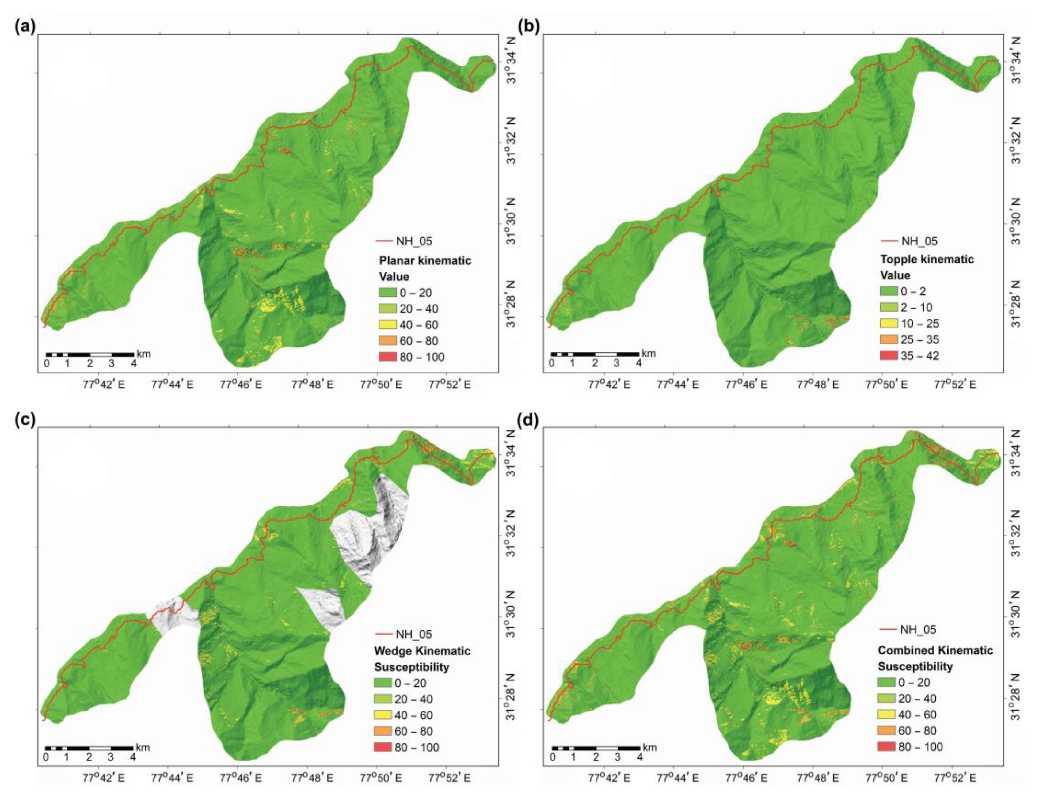
Table A2. Quantitative information on the number of pixels susceptible for each mode and all types of failure separately & combined for all sets of discontinuities.
Susceptibility RangePixels Susceptible to Planar Failure (|% of Total Pixels)Pixels Susceptible to Topple Failure (|% of Total Pixels)
Joint 1Joint 2Joint 3All Joint SetsJoint 1Joint 2Joint 3All Joint Sets
0–20610.0190.0070.00770.0138960.6067951.0424210.3713,1122.02
21–4031580.495750.0913740.2151020.785810.0913330.201160.0220300.31
41–6044550.6918890.2945880.7110,8691.67320.002640.0430.002990.05
61–8012450.1922800.3527220.4262150.96
81–1002070.036820.107400.1116280.25
failed91261.4054350.8494311.4523,8913.6745090.6983921.2925400.3915,4412.37
stable641,18598.60644,87699.16640,88098.55626,42096.33645,80299.31641,91998.71647,77199.61634,87097.63
Susceptibility RangePixels Susceptible to Wedge Failure (|% of Total Pixels)Combined Types of FailurePlanar to All Mode %Topple to All Mode %Wedge to All Mode %
Joint 1&2Joint 1&3Joint 2&3All
Intersections
All Failure% of Total
Pixels
0–2024790.3825250.3943070.6674911.1516,8042.580.4678.0344.58
21–4027500.4238670.5939090.6086481.3314,8442.2834.3713.6858.26
41–6018950.2929560.4535950.5572131.1118,1002.7860.051.6539.85
61–8014200.228630.1314400.2235220.5497201.4963.9436.23
81–1008600.131950.033300.0513800.2130070.4654.1445.89
failed94041.4510,4061.6013,5812.0928,2544.3462,4759.6138.2424.7245.22
stable640,90798.55639,90598.40636,73097.91622,05795.66587,83690.39Total number of pixels = 650,311

References

  1. Rechberger, C.; Fey, C.; Zangerl, C. Structural characterisation, internal deformation, and kinematics of an active deep-seated rockslide in a valley glacier retreat area. Eng. Geol. 2021, 286, 106048. [Google Scholar] [CrossRef]
  2. Cruden, D.M.; Hu, X.Q. Exhaustion and steady state models for predicting landslide hazards in the Canadian Rocky Mountains. Geomorphology 1993, 8, 279–285. [Google Scholar] [CrossRef]
  3. Agliardi, F.; Crosta, G.; Zanchi, A. Structural constraints on deep-seated slope deformation kinematics. Eng. Geol. 2001, 59, 83–102. [Google Scholar] [CrossRef]
  4. Grelle, G.; Revellino, P.; Donnarumma, A.; Guadagno, F.M. Bedding control on landslides: A methodological approach for computer-aided mapping analysis. Nat. Hazards Earth Syst. Sci. 2011, 11, 1395–1409. [Google Scholar] [CrossRef]
  5. Travelletti, J.; Malet, J.P.; Samyn, K.; Grandjean, G.; Jaboyedoff, M. Control of landslide retrogression by discontinuities: Evidence by the integration of airborne- and ground-based geophysical information. Landslides 2013, 10, 37–54. [Google Scholar] [CrossRef]
  6. Břežný, M.; Pánek, T. Deep-seated landslides affecting monoclinal flysch morphostructure: Evaluation of LiDAR-derived topography of the highest range of the Czech Carpathians. Geomorphology 2017, 285, 44–57. [Google Scholar] [CrossRef]
  7. Gupta, V.; Solanki, A.; Jagtap, S.; Joshi, M.; Bhakuni, S.S. Morpho-structural approach to assess landslides in the Kali river valley, NE Kumaun Himalaya, India. Environ. Earth Sci. 2022, 81, 35. [Google Scholar] [CrossRef]
  8. Cruden, D.M.; Eaton, T.M. Reconnaissance of rockslide hazards in Kananaskis Country, Alberta. Can. Geotech. J. 1987, 24, 414–429. [Google Scholar] [CrossRef]
  9. Goodman, R.E.; Bray, J.W. Toppling of rock slopes. In Proceedings of the Specialty Conference on Rock Engineering for Foundations and Slopes, Boulder, CO, USA, 15–18 August 1976; Volume 2, pp. 201–223. [Google Scholar]
  10. Hoek, E.; Bray, J.W. Rock Slope Engineering, 3rd ed.; The Institution of Mining and Metallurgy: London, UK, 1981; pp. 341–351. [Google Scholar]
  11. Matheson, G.D. Rock Stability Assessment in Preliminary Site Investigations—Graphical Methods; Report 1039; Transport and Road Research Laboratory: Crownthorne, UK, 1983. [Google Scholar]
  12. Kundu, J.; Sarkar, K.; Singh, A.K. Integrating structural and numerical solutions for road cut slope stability analysis: A case study, India. In Rock Dynamics: From Research to Engineering; CRC Press: Boca Raton, FL, USA, 2016; pp. 457–462. [Google Scholar] [CrossRef]
  13. Cundall, P.A.; Hart, R.D. Numerical modelling of discontinua. Eng. Comput. 1992, 9, 101–113. [Google Scholar] [CrossRef]
  14. Hammah, R.; Yacoub, T.; Corkum, B. The practical modelling of discontinuous rock masses with finite element analysis. In 42nd US Rock Mechanics Symposium and 2nd U.S.-Canada Rock Mechanics Symposium; American Rock Mechanic Association, Curran Associates, Inc.: Red Hook, NY, USA, 2008; pp. 56–63. [Google Scholar]
  15. Kundu, J.; Mahanta, B.; Tripathy, A.; Sarkar, K.; Singh, T.N. Stability Evaluation of Jointed Rock Slope with Curved Face. INDOROCK-2016. In Proceedings of the 6th Indian Rock Conference June 17-18 IIT Bombay, Jointly Organized by Indian Institute of Technology Mumbai and Indian Society of Rock Mechanics and Tunneling Technology, Mumbai, India, 17–18 June 2016; pp. 971–978. [Google Scholar]
  16. Siad, L.; Megueddem, M. Stability analysis of jointed rock slope. Mech. Res. Commun. 1998, 25, 661–670. [Google Scholar] [CrossRef]
  17. Jaboyedoff, M.; Choffet, M.; Derron, M.H.; Horton, P.; Loye, A.; Longchamp, C.; Mazotti, B.; Michoud, C.; Pedrazzini, A. Preliminary slope mass movement susceptibility mapping using DEM and lidar DEM. In Terrigenous Mass Movements: Detection, Modelling, Early Warning and Mitigation Using Geoinformation Technology; Springer: Berlin/Heidelberg, Germany, 2012; Volume 9783642254956, pp. 109–170. [Google Scholar] [CrossRef]
  18. Romstad, B.; Harbitz, C.B.; Domaas, U. A GIS method for assessment of rock slide tsunami hazard in all Norwegian lakes and reservoirs. Hazards Earth Syst. Sci. 2009, 9, 353–364. Available online: www.nat-hazards-earth-syst-sci.net/9/353/2009/ (accessed on 10 January 2023). [CrossRef]
  19. Terzaghi, R.D. Sources of error in joint surveys. Géotechnique 1965, 15, 287–304. [Google Scholar] [CrossRef]
  20. Meentemeyer, R.K.; Moody, A. Automated mapping of conformity between topographic and geological surfaces. Comput. Geosci. 2000, 26, 815–829. [Google Scholar] [CrossRef]
  21. Mishra, B.K.; Bhattacharjee, D.; Chattopadhyay, A.; Prusty, G. Tectonic and lithologic control over landslide activity within the Larji–Kullu Tectonic Window in the Higher Himalayas of India. Nat. Hazards 2018, 92, 673–697. [Google Scholar] [CrossRef]
  22. Šilhán, K.; Pánek, T.; Škarpich, V.; Břežný, M.; Chalupa, V. Specifics of slope movements on slopes with contrasting structural conditions: Evidence from tree-ring records. Geomorphology 2022, 415, 108425. [Google Scholar] [CrossRef]
  23. Günther, A. SLOPEMAP: Programs for automated mapping of geometrical and kinematical properties of hard rock hill slopes. Comput. Geosci. 2003, 29, 865–875. [Google Scholar] [CrossRef]
  24. Aksoy, H.; Ercanoglu, M. Fuzzified kinematic analysis of discontinuity-controlled rock slope instabilities. Eng. Geol. 2007, 89, 206–219. [Google Scholar] [CrossRef]
  25. Santangelo, M.; Marchesini, I.; Cardinali, M.; Fiorucci, F.; Rossi, M.; Bucci, F.; Guzzetti, F. A method for the assessment of the influence of bedding on landslide abundance and types. Landslides 2015, 12, 295–309. [Google Scholar] [CrossRef]
  26. Park, H.J.; Lee, J.H.; Kim, K.M.; Um, J.G. Assessment of rock slope stability using GIS-based probabilistic kinematic analysis. Eng. Geol. 2016, 203, 56–69. [Google Scholar] [CrossRef]
  27. Park, H.J.; West, T.R. Development of a probabilistic approach for rock wedge failure. Eng. Geol. 2001, 59, 233–251. [Google Scholar] [CrossRef]
  28. Yoon, W.S.; Jeong, U.J.; Kim, J.H. Kinematic analysis for sliding failure of multi-facedrock slopes. Eng. Geol. 2002, 67, 51–61. [Google Scholar] [CrossRef]
  29. Singh, D.; Singh, P.K.; Kainthola, A.; Pandey, H.K.; Kumar, S.; Singh, T.N. Analysis of failure pattern in cut slopes of bedded sandstone: A case study. Environ. Earth Sci. 2022, 81, 398. [Google Scholar] [CrossRef]
  30. Admassu, Y.; Shakoor, A. DIPANALYST: A computer program for quantitative kinematic analysis of rock slope failures. Comput. Geosci. 2013, 54, 196–202. [Google Scholar] [CrossRef]
  31. Kundu, J.; Sarkar, K.; Verma, A.K.; Singh, T.N. Novel methods for quantitative analysis of kinematic stability and slope mass rating in jointed rock slopes with the aid of a new computer application. Bull. Eng. Geol. Environ. 2022, 81, 29. [Google Scholar] [CrossRef]
  32. Smith, J.V. A method for assessing discontinuity poles for potential wedge sliding. Eng. Geol. 2016, 202, 55–61. [Google Scholar] [CrossRef]
  33. Zheng, J.; Lü, Q.; Deng, J.; Yang, X.; Fan, X.; Ding, Z. A modified stereographic projection approach and a free software tool for kinematic analysis of rock slope toppling failures. Bull. Eng. Geol. Environ. 2019, 78, 4757–4769. [Google Scholar] [CrossRef]
  34. Tatone, B.S.A.; Grasselli, G. ROCKTOPPLE: A spreadsheet-based program for probabilistic block-toppling analysis. Comput. Geosci. 2010, 36, 98–114. [Google Scholar] [CrossRef]
  35. Zheng, J.; Kulatilake, P.H.S.W.; Asce, F.; Shu, B. Improved Probabilistic Kinematic Analysis Procedure Based on Finite Size Discontinuities and Its Application to a Rock Slope at Open Pit Mine in U.S. Int. J. Geomech. 2016, 17, 04016052. [Google Scholar] [CrossRef]
  36. Zhou, X.; Chen, J.; Chen, Y.; Song, S.; Shi, M.; Zhan, J. Bayesian-based probabilistic kinematic analysis of discontinuity-controlled rock slope instabilities. Bull. Eng. Geol. Environ. 2017, 76, 1249–1262. [Google Scholar] [CrossRef]
  37. Obregon, C.; Mitri, H. Probabilistic approach for open pit bench slope stability analysis—A mine case study. Int. J. Min. Sci. Technol. 2019, 29, 629–640. [Google Scholar] [CrossRef]
  38. Yan, J.; Chen, J.; Li, Y.; Li, Z.; Zhang, Y.; Zhou, X.; Mehmood, Q.; Liu, J.; Wang, Z. Kinematic-based failure angle analysis for discontinuity-controlled rock slope instabilities: A case study of Ren Yi Peak Cluster in Fusong County, China. Nat. Hazards 2022, 111, 2281–2296. [Google Scholar] [CrossRef]
  39. Rusydy, I.; Mulkal, M.; Baramsyah, H.; Ahmadian, H.; Hussin, H.; Al-Huda, N.; Marwan, M. Rock slope kinematic analysis for planar failure: A probabilistic approach. E3S Web Conf. 2022, 340, 01017. [Google Scholar] [CrossRef]
  40. Genevois, R.; Romeo, R.W.; Scarascia Mugnozza, G. Un approccio probabilistico all’analisi di stabilita di versanti in roccia. Geol. Rom. 1987, 26, 263–286. [Google Scholar]
  41. Ismail, A.; Ahmad Safuan, A.R.; Sa’ari, R.; Wahid Rasib, A.; Mustaffar, M.; Asnida Abdullah, R.; Kassim, A.; Mohd Yusof, N.; Abd Rahaman, N.; Kalatehjari, R. Application of combined terrestrial laser scanning and unmanned aerial vehicle digital photogrammetry method in high rock slope stability analysis: A case study. Meas. J. Int. Meas. Confed. 2022, 195, 111161. [Google Scholar] [CrossRef]
  42. Leung, C.F.; Kheok, S.C. Computer Aided Analysis of Rock Slope Stability. Rock Mech. Rock Eng. 1987, 20, 111–122. [Google Scholar] [CrossRef]
  43. Bonham-Carter, G.F. Geographic Information Systems for Geoscientists: Modelling with GIS; Pergamon, Elsevier Ltd.: Amsterdam, The Netherlands, 1994; p. 398. [Google Scholar] [CrossRef]
  44. Chorowicz, J.; Breard, J.Y.; Guillande, R.; Morasse, C.R.; Prudon, D.; Rudant, J.P. Dip and strike measured systematically on digitised three-dimensional geological maps. Photogramm. Eng. Remote Sens. 1991, 57, 431–436. [Google Scholar]
  45. Chorowicz, J.; Parrot, J.F.; Taud, H.; Hakdaoui, H.; Rudant, J.P.; Rouis, T. Automated pattern-recognition of geomorphic features from DEMS and satellite images. Z. Fur Geomorphol. 1995, 101, 69–84. [Google Scholar]
  46. Pack, R.T.; Tarboton, D.G.; Goodwin, C.N. The SINMAP Approach to Terrain Stability Mapping. In Proceedings of the 8th Congress of the International Association of Engineering Geology, Vancouver, BC, Canada, 21–25 September 1998; Volume 2, pp. 1157–1166. [Google Scholar]
  47. de Kemp, E.A. Three-dimensional projection of curvilinear geological features through direction cosine interpolation of structural field observations. Comput. Geosci. 1998, 24, 269–284. [Google Scholar] [CrossRef]
  48. de Kemp, E.A. Visualisation of complex geological structures using 3-D Bezier construction tools. Comput. Geosci. 1999, 25, 581–597. [Google Scholar] [CrossRef]
  49. Gunther, A.; Carstensen, A.; Pohl, W. Automated sliding susceptibility mapping of rock slopes. Nat. Hazards Earth Syst. Sci. 2004, 4, 95–102. [Google Scholar] [CrossRef]
  50. Günther, A.; Wienhöfer, J.; Konietzky, H. Automated mapping of rock slope geometry, kinematics and stability with RSS-GIS. Nat. Hazards 2012, 61, 29–49. [Google Scholar] [CrossRef]
  51. Ghosh, S.; Günther, A.; Carranza, E.J.M.; van Westen, C.J.; Jetten, V.G. Rock slope instability assessment using spatially distributed structural orientation data in Darjeeling Himalaya (India). Earth Surf. Process. Landf. 2010, 35, 1773–1792. [Google Scholar] [CrossRef]
  52. Ghosh, S.; Kumar, A.; Bora, A. Analysing the stability of a failing rock slope for suggesting suitable mitigation measure: A case study from the Theng rockslide, Sikkim Himalayas, India. Bull. Eng. Geol. Environ. 2014, 73, 931–945. [Google Scholar] [CrossRef]
  53. Ji, J.; Wang, C.-W.; Cui, H.-Z.; Li, X.-Y.; Song, J.; Gao, Y. A simplified nonlinear coupled Newmark displacement model with degrading yield acceleration for seismic slope stability analysis. Int. J. Numer. Anal. Methods Geomech. 2021, 45, 1303–1322. [Google Scholar] [CrossRef]
  54. Dadon, A.; Peeters, A.; Ben-Dor, E.; Karnieli, A. A semi-automated GIS model for extracting geological structural information from a spaceborne thematic image. GISci Remote Sens. 2011, 48, 264–279. [Google Scholar] [CrossRef]
  55. Matasci, B.; Stock, G.M.; Jaboyedoff, M.; Carrea, D.; Collins, B.D.; Guérin, A.; Matasci, G.; Ravanel, L. Assessing rockfall susceptibility in steep and overhanging slopes using three-dimensional analysis of failure mechanisms. Landslides 2018, 15, 859–878. [Google Scholar] [CrossRef]
  56. Rowe, E.; Hutchinson, D.J.; Kromer, R.A. An analysis of failure mechanism constraints on pre-failure rock block deformation using TLS and roto-translation methods. Landslides 2018, 15, 409–421. [Google Scholar] [CrossRef]
  57. Konstantinidis, I.; Marinos, V.; Papathanassiou, G. UAV-Based Evaluation of Rockfall Hazard in the Cultural Heritage Area of Kipinas Monastery, Greece. Appl. Sci. 2021, 11, 8946. [Google Scholar] [CrossRef]
  58. Menegoni, N.; Giordan, D.; Perotti, C. An Open-Source Algorithm for 3D ROck Slope Kinematic Analysis (ROKA). Appl. Sci. 2021, 11, 1698. [Google Scholar] [CrossRef]
  59. Gigli, G.; Lombardi, L.; Carlà, T.; Beni, T.; Casagli, N. A method for full three-dimensional kinematic analysis of steep rock walls based on high-resolution point cloud data. Int. J. Rock Mech. Min. 2022, 157, 105178. [Google Scholar] [CrossRef]
  60. Eberhardt, E.; Stead, D.; Coggan, J.S. Numerical analysis of initiation and progressive failure in natural rock slopes-the 1991 Randa rockslide. Int. J. Rock Mech. Min. 2004, 41, 69–87. [Google Scholar] [CrossRef]
  61. Leung, C.F.; Quek, S.T. Probabilistic stability analysis of excavations in jointed rock. Can. Geotech. J. 1995, 32, 397–407. [Google Scholar] [CrossRef]
  62. Romana, M. New adjustment ratings for application of Bieniawski classification to slopes. In Proceedings of the International Symposium on the role of rock mechanics, ISRM, Zacatecas, Mexico, 2–4 September 1985; pp. 49–53. [Google Scholar]
  63. Sarkar, K.; Kumar Singh, A.; Niyogi, A.; Kumar Behera, P.; Verma, A.K.; Singh, T.N. The Assessment of Slope Stability along NH-22 in Rampur-Jhakri Area, Himachal Pradesh. J. Geol. Soc. India 2016, 88, 387–393. [Google Scholar] [CrossRef]
  64. Siddique, T.; Masroor Alam, M.; Mondal, M.E.A.; Vishal, V. Slope mass rating and kinematic analysis of slopes along the national highway-58 near Jonk, Rishikesh, India. J. Rock Mech. Geotech. Eng. 2015, 7, 600–606. [Google Scholar] [CrossRef]
  65. Bieniawski, Z.T. Engineering Rock Mass Classifications: A Complete Manual for Engineering and Geologists in Mining, Civil and Petroleum Engineering; Wiley: Chichester/London, UK, 1989. [Google Scholar]
  66. Anbalagan, R.; Sharma, S.; Raghuvanshi, T.K. Rock mass stability evaluation using Modified SMR Approach. In Proceedings of the 6th Natural Symposium on Rock Mechanics, Bangalore, India, 15 June 1992; pp. 258–268. [Google Scholar]
  67. Tomás, R.; Delgado, J.; Serón, J.B. Modification of slope mass rating (SMR) by continuous functions. Int. J. Rock Mech. Min. 2007, 44, 1062–1069. [Google Scholar] [CrossRef]
  68. Singh, K. Deformation history of the rocks around Sarahan Bushair, Himachal Pradesh. In Structural Geology of the Himalaya; Saklani, P.S., Ed.; Today and Tomorrow’s Printers & Publishers: Darya, India, 1979; pp. 163–182. [Google Scholar]
  69. Pandey, A.K.; Sachan, H.K.; Virdi, N.S. Exhumation history of a shear zone constrained by microstructural and fluid inclusion techniques: An example from the Satluj valley, NW Himalaya, Indian. J. Asian Earth Sci. 2004, 23, 391–406. [Google Scholar] [CrossRef]
  70. Bhargava, O.N.; Kaur, G.; Deb, M. A Paleoproterozoic paleosol horizon in the Lesser Himalaya and its regional implications. J. Asian Earth Sci. 2011, 42, 1371–1380. [Google Scholar] [CrossRef]
  71. Mukhopadhaya, D.K.; Ghosh, T.K.; Bhadra, B.K.; Srivastava, D.C. Structural and metamorphic evolution of the rocks of the Jutogh Group, Chur half-klippe, Himachal Himalayas: A summary and comparison with the Simla area. Proc. Indian Acad. Sci.—Earth Planet. Sci. 1997, 106, 197–207, Published by Indian Academy of Sciences. [Google Scholar] [CrossRef]
  72. Srikantia, S.V.; Bhargava, O.N. Geology of Himachal Pradesh; Geological Society of India: Bangalore, India, 1998; pp. 1–408. [Google Scholar]
  73. Draganits, E.; Grasemann, B.; Janda, C.; Hager, C.; Preh, A. 300MW Baspa II—India’s largest private hydroelectric facility on top of a rock avalanche-dammed palaeo-lake (NW Himalaya): Regional geology, tectonic setting and seismicity. Eng. Geol. 2014, 169, 14–29. [Google Scholar] [CrossRef]
  74. Marchesini, I.; Santangelo, M.; Fiorucci, F.; Cardinali, M.; Rossi, M.; Guzzetti, F. A GIS Method for Obtaining Geologic Bedding Attitude. In Landslide Science and Practice; Margottini, C., Canuti, P., Sassa, K., Eds.; Springer: Berlin/Heidelberg, Germany, 2013. [Google Scholar] [CrossRef]
  75. Marchesini, I.; Santangelo, M.; Fiorucci, F.; Cardinali, M.; Rossi, M.; Bucci, F.; Guzzetti, F. TXT-tool 1.039-1.2 Bedding Attitude Information through the Interpretation of Stereoscopic Aerial Photographs and GIS Modeling. In Landslide Dynamics: ISDR-ICL Landslide Interactive Teaching Tools; Springer: Cham, Switzerland, 2018; pp. 175–186. [Google Scholar] [CrossRef]
  76. Msaddek, M.H.; Moumni, Y.; Chenini, I.; Dlala, M. Applicability of Developed Algorithm for Semi-automated Extraction and Morphotectonic Interpretation of Lineaments Using Remotely Sensed Data, Southwestern Tunisia. Remote Sens. Earth Sys. Sci. 2019, 2, 292–307. [Google Scholar] [CrossRef]
  77. Matherson, G.D. The collection and use of field discontinuity data in rock slope design. Quart J. Eng. Geol. 1989, 22, 19–30. [Google Scholar] [CrossRef]
  78. Wyllie, D.; Mah, C. Rock Slope Engineering; CRC Press: London, UK, 2004. [Google Scholar] [CrossRef]
  79. Skilodimou, H.D.; Bathrellos, G.D.; Koskeridou, E.; Soukis, K.; Rozos, D. Physical and Anthropogenic Factors Related to Landslide Activity in the Northern Peloponnese, Greece. Land 2018, 7, 85. [Google Scholar] [CrossRef]
  80. Karpouza, M.; Chousianitis, K.; Bathrellos, G.D.; Skilodimou, H.D.; Kaviris, G.; Antonarakou, A. Hazard zonation mapping of earthquake-induced secondary effects using spatial multi-criteria analysis. Nat. Hazards 2021, 109, 637–669. [Google Scholar] [CrossRef]
  81. Ji, J.; Cui, H.; Zhang, T.; Song, J.; Gao, Y. A GIS-based tool for probabilistic physical modelling and prediction of landslides: GIS-FORM landslide susceptibility analysis in seismic areas. Landslides 2022, 19, 2213–2231. [Google Scholar] [CrossRef]
  82. Bathrellos, G.D.; Skilodimou, H.D. Land Use Planning for Natural Hazards. Land 2019, 8, 128. [Google Scholar] [CrossRef]
  83. Fawcett, T. An introduction to ROC analysis. Pattern Recognit. Lett. 2006, 27, 861–874. [Google Scholar] [CrossRef]
  84. Conforti, M.; Ietto, F. Modeling Shallow Landslide Susceptibility and Assessment of the Relative Importance of Predisposing Factors, through a GIS-Based Statistical Analysis. Geosciences 2021, 11, 333. [Google Scholar] [CrossRef]
  85. Mohapatra, S.R.; Kohli, A.; Thakur, V.; Poonia, A. A Field Note on the Reconnaissance Study of a Rockslide Incidence of 11/08/2021 at NH-05, Near Nigulsari Village, Tehsil Nichar, District Kinnaur, Himachal Pradesh. 2021. Available online: https://employee.gsi.gov.in/cs/groups/public/documents/document/dmkx/mdm2/~edisp/dcport1gsigovi1036481.pdf (accessed on 10 January 2023).
  86. Nishat; Tariq, Q.A. Geological Assessment of Landslide/Slope Failure Incidence Near Jeori (Nh-05) Road, District Shimla, Himachal Pradesh. 2021. Available online: https://employee.gsi.gov.in/cs/groups/public/documents/document/dmkx/mdm2/~edisp/dcport1gsigovi1036480.pdf (accessed on 10 January 2023).
  87. Kundu, J. Stability Evaluation of Hill Slopes: New Perspectives to Rock Material and Rock Mass Characterisation. Ph.D. Thesis, Indian Institute of Technology (ISM), Dhanbad, India, 2020. [Google Scholar]
  88. Kundu, J.; Sarkar, K.; Singh, A.K.; Singh, T.N. Continuous functions and a computer application for Rock Mass Rating. Int. J. Rock Mech. Min. 2020, 129, 104280. [Google Scholar] [CrossRef]
Figure 1. Description of the angular relationships between joints and slope surface for planar, wedge, and flexural topple conditions. The X stands for α, β, or γ (angular relationship determinant) described in the figure.
Land 12 00402 g001
Figure 2. Geological map of the study area.
Land 12 00402 g002
Figure 3. A screenshot of GISMR GUI showing all the input options and function buttons designed in the application.
Land 12 00402 g003
Figure 4. Flowchart of GISMR for kinematic analysis describing the calculation process for planar, topple, and wedge failure.
Land 12 00402 g004
Figure 5. Workflow for determination of structural stability in a large region using GISMR.
Land 12 00402 g005
Figure 6. (a) Pole plot of all the discontinuities on a stereographic net showing the major orientation of discontinuity sets 1, 2 and 3. (b) representation of structurally homogenous zones within the small grey polygon boundaries draped over the hill shade layer derived from DEM. (c) Interpolated dip map of joint-1 in the area (IDW with barriers of joint zones and structural defects) (d) Interpolated dip direction map of joint-1 in the area (IDW interpolation with barriers of joint zones and structural defects).
Land 12 00402 g006
Figure 7. The screenshot of the GISMR application shows “Plane To Cosines” function, which is capable of importing planar or linear orientations in a text file in dip and dip direction format and converting into cosine values.
Land 12 00402 g007
Figure 8. (a) Slope map of the area, (b) Aspect map of the area derived from DEM. The values in the legend are in degrees.
Land 12 00402 g008
Figure 9. Kinematic susceptibility results (maximum value out of all the layers at each pixel) from the combined effect of all joint sets for (a) planar failure susceptibility; (b) topple failure susceptibility; (c) wedge failure susceptibility; (d) all modes of failure (combined) susceptibility.
Land 12 00402 g009
Figure 10. Results of slope optimisation: (a) the pixel value represents the slope value needed to maintain a kinematic susceptibility value of 50; (b) pixels with negative values need to be flattened by the amount subtracted from the slope angle. Pixels with a positive value may be steepened maximally by the amount indicated without compromising safety.
Land 12 00402 g010
Figure 11. Landslide inventory of the study area. Each landslide in the area is outlined in a black line and filled with cyan colour. The red line represents the national highway 05 that passes through the study region.
Land 12 00402 g011
Figure 12. Frequency ratio (FR) for different joint and intersection sets in each mode of kinematic failure: (a) planar: the higher FR of joint 2 represents its dominance in creating planar failures; (b) topple: joint 1 is responsible for maximum flexural topple failures; (c) wedge: failure along joints 1 and 3 intersection is dominant for the slopes with susceptibility less than 80 and failures along joints 2 and 3 intersection are dominant for slopes with susceptibility more than 80; (d) FR comparison for failures due to different modes of failure suggests that wedge failure is the dominant type of failure followed by planar and topple.
Land 12 00402 g012
Figure 13. The ROC curve for the kinematics susceptibility analysis.
Land 12 00402 g013
Figure 14. (a) Kinematic susceptibility map draped over Google Earth (GE) view showing locations of Nigulsari and Jeori landslide; (b) GE image before occurrence of Jeori landslide; (c) GE image post failure clearly shows signs of disturbance; (d) Susceptibility map overlain on GE view shows the zone is highly to very-highly susceptible to kinematic failure.
Land 12 00402 g014
Figure 15. (a) Panoramic view of Nigulsari rockslide along National Highway 05; (b) affected slope down the highway shows highly unfavourable discontinuity orientations; (c) the failed portion was analysed to be highly to very-highly susceptible to kinematic failure.
Land 12 00402 g015
Disclaimer/Publisher’s Note: The statements, opinions and data contained in all publications are solely those of the individual author(s) and contributor(s) and not of MDPI and/or the editor(s). MDPI and/or the editor(s) disclaim responsibility for any injury to people or property resulting from any ideas, methods, instructions or products referred to in the content.

