
Time Series Analyses and Forecasting of Surface Urban Heat Island Intensity Using ARIMA Model in Punjab, Pakistan
 ,
,  ,
,
Abstract
:1. Introduction
2. Materials and Methods
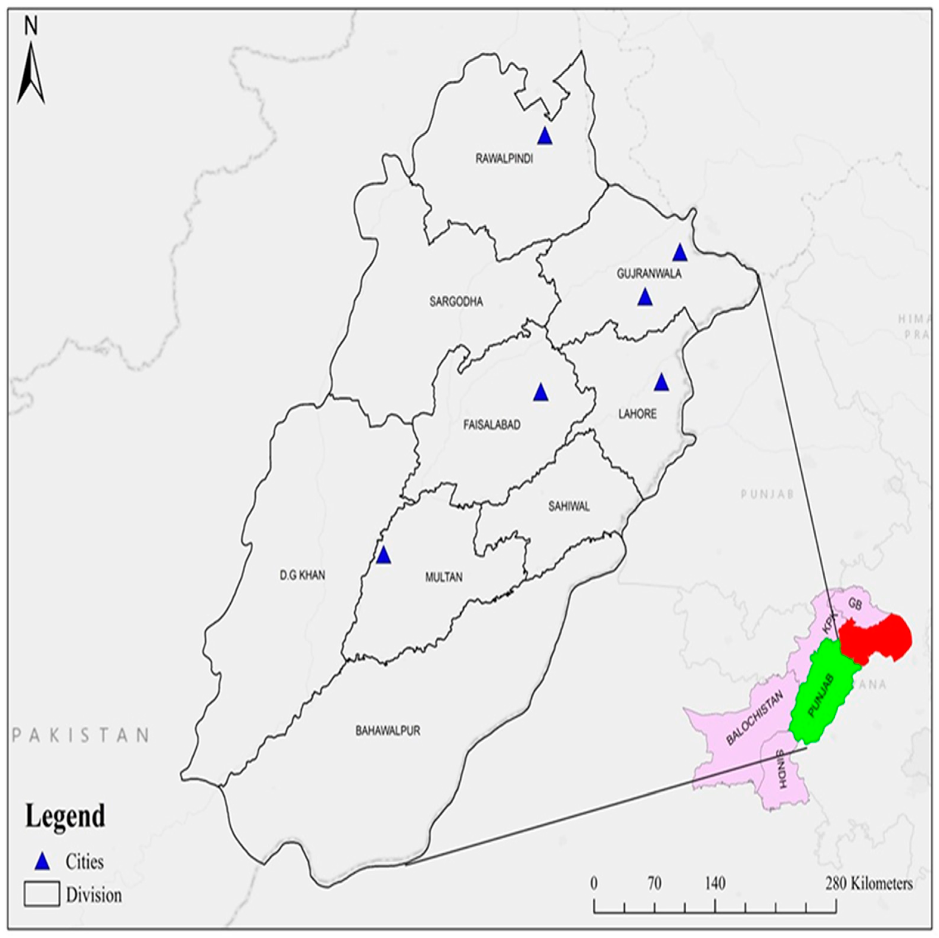
2.1. Study Area
2.2. Data
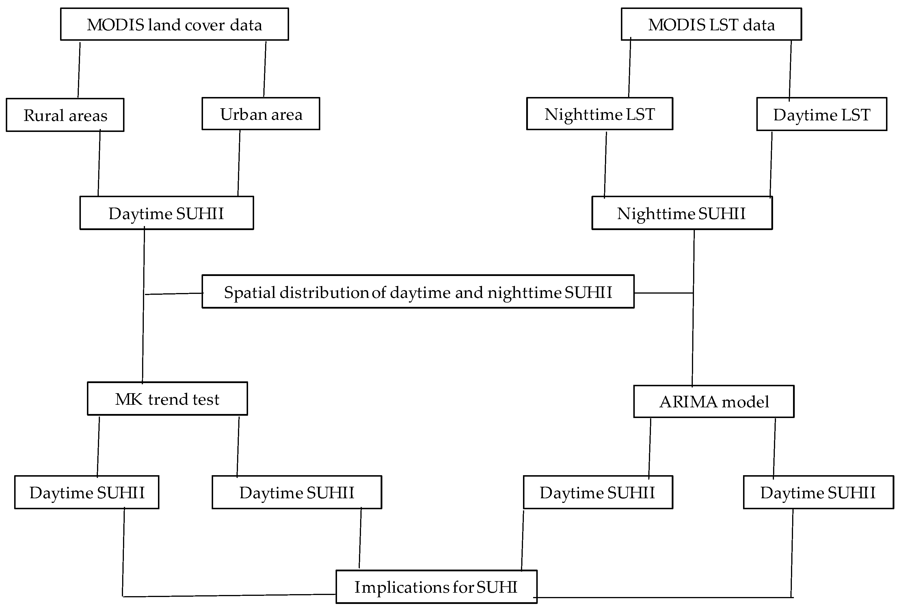
2.3. Methods
2.3.1. Delineation of Rural and Urban Areas
2.3.2. SUHII Calculation
2.3.3. Mann-Kendall Test for Trend
2.3.4. Sen’s Slope Estimator
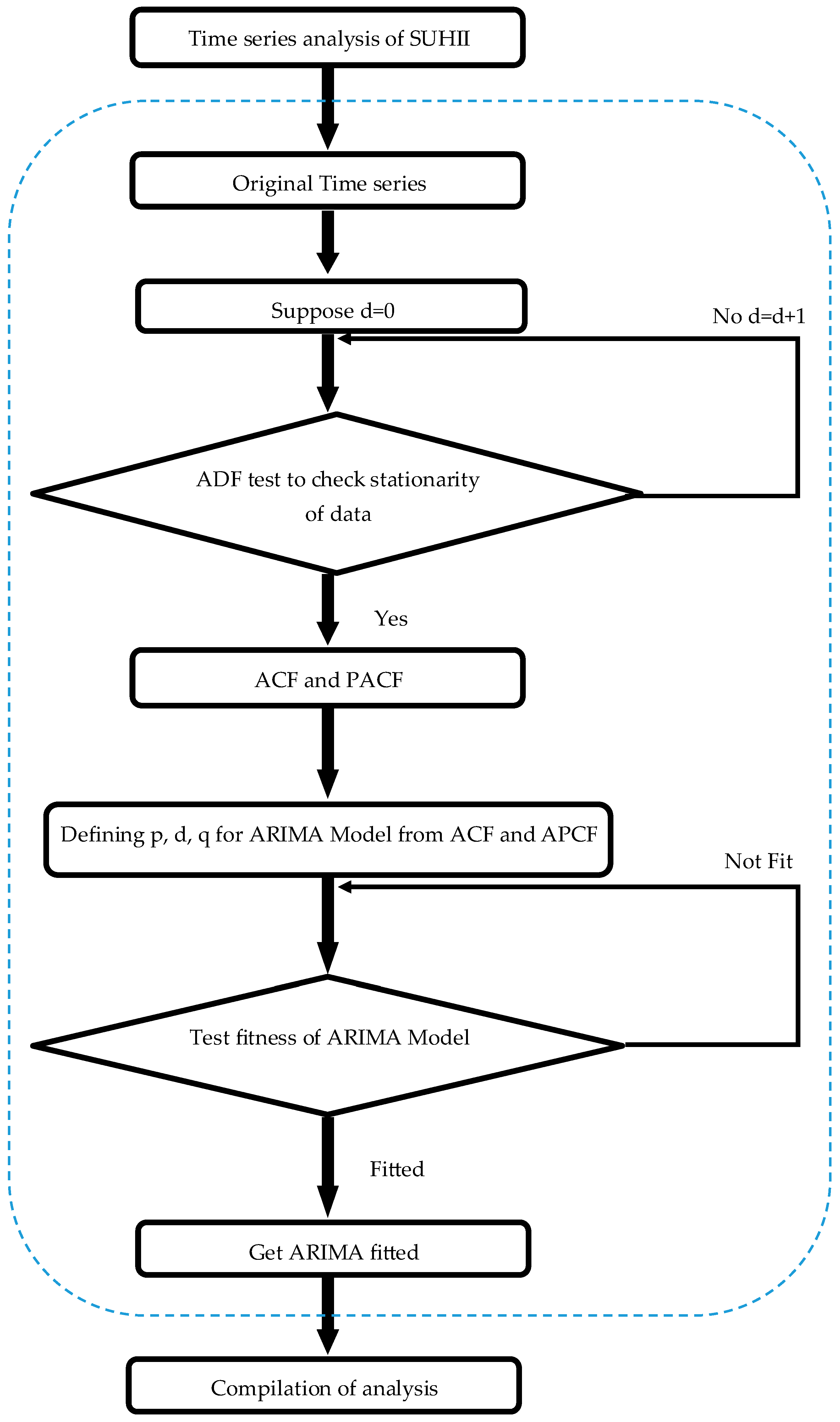
2.4. ARIMA Modeling
3. Results
3.1. Distribution of the Average SUHII for the Last 15 Years
3.2. Statistical Summary of SUHII
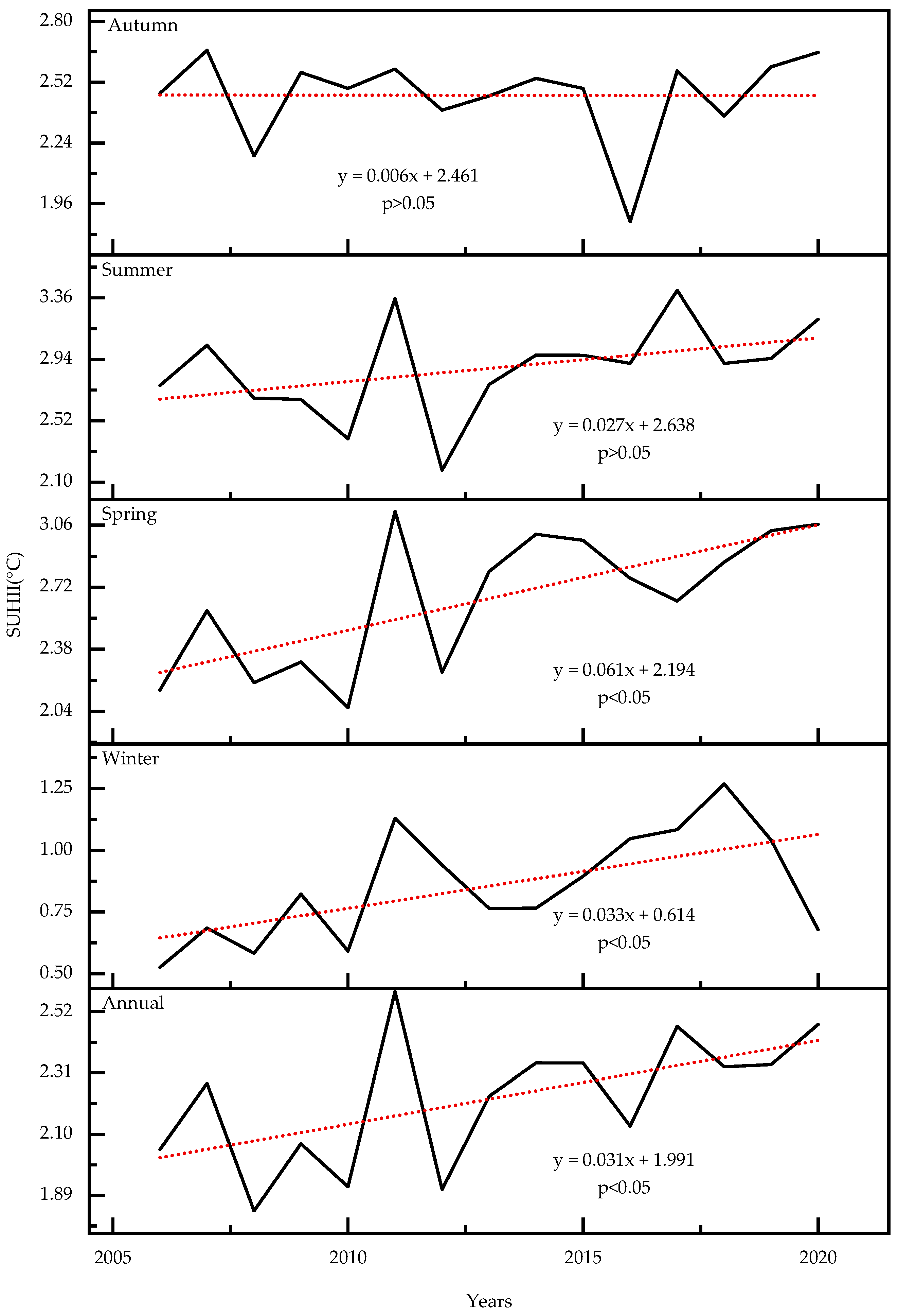
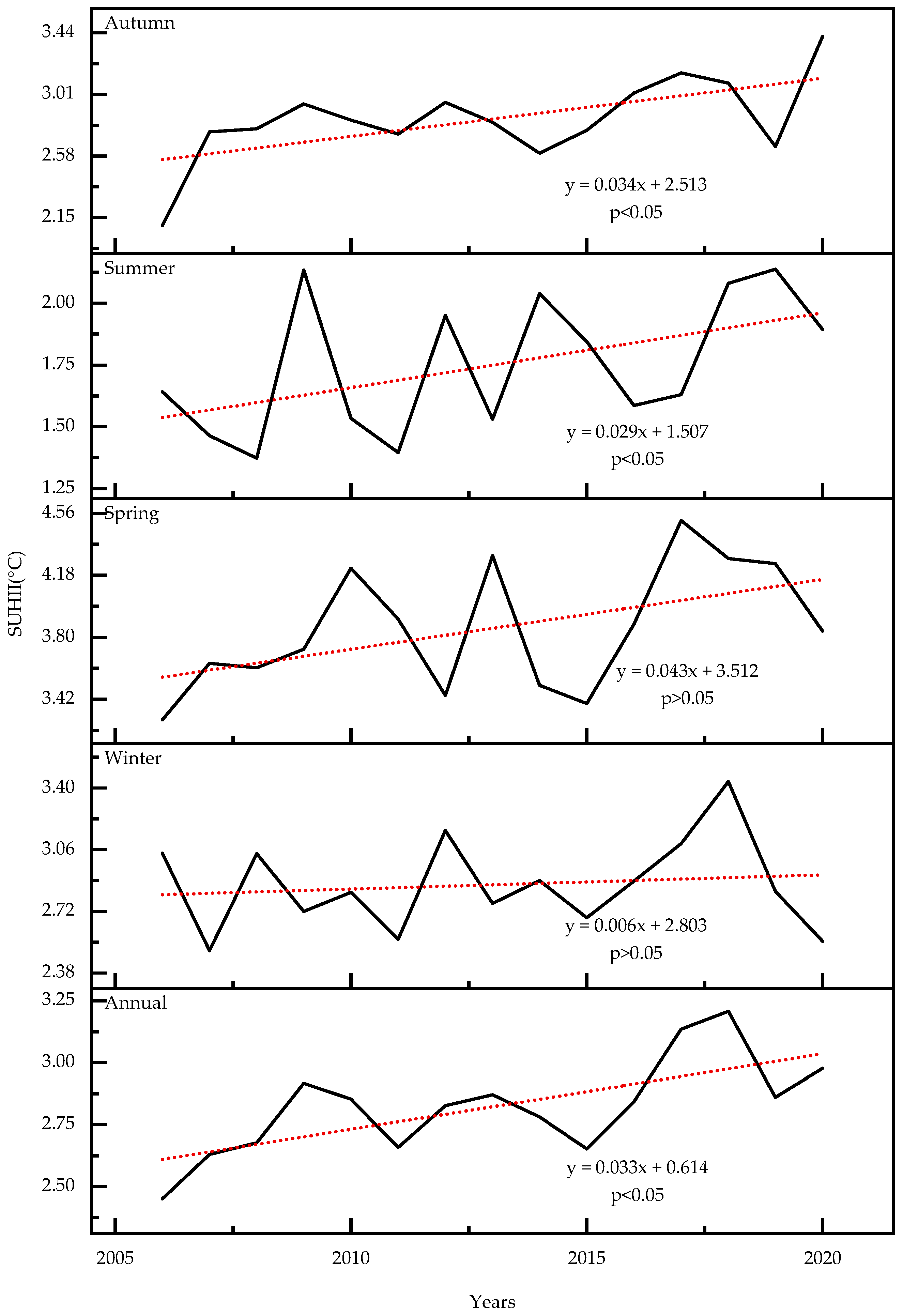
3.3. Fifteen-Year Temporal Trends of SUHII for Punjab
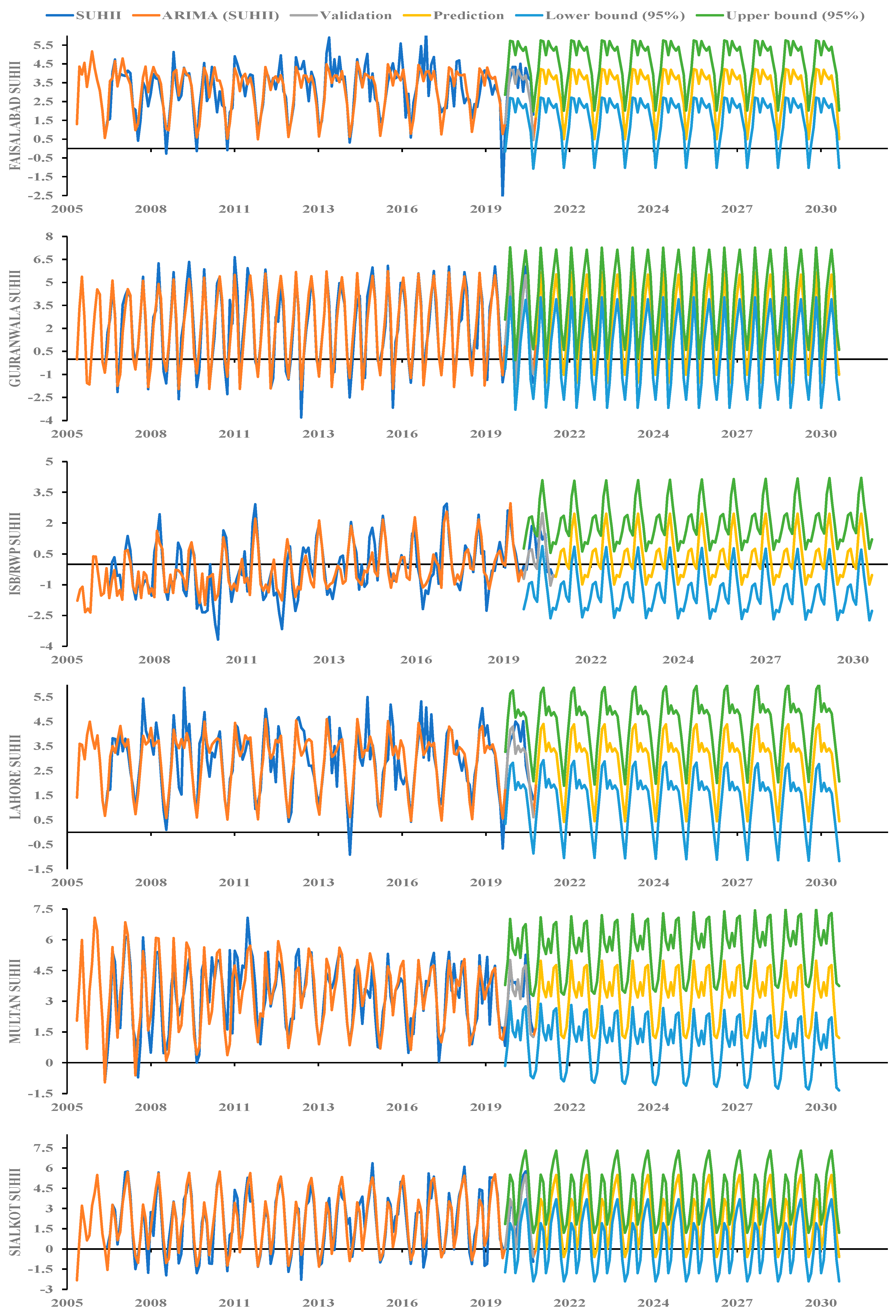
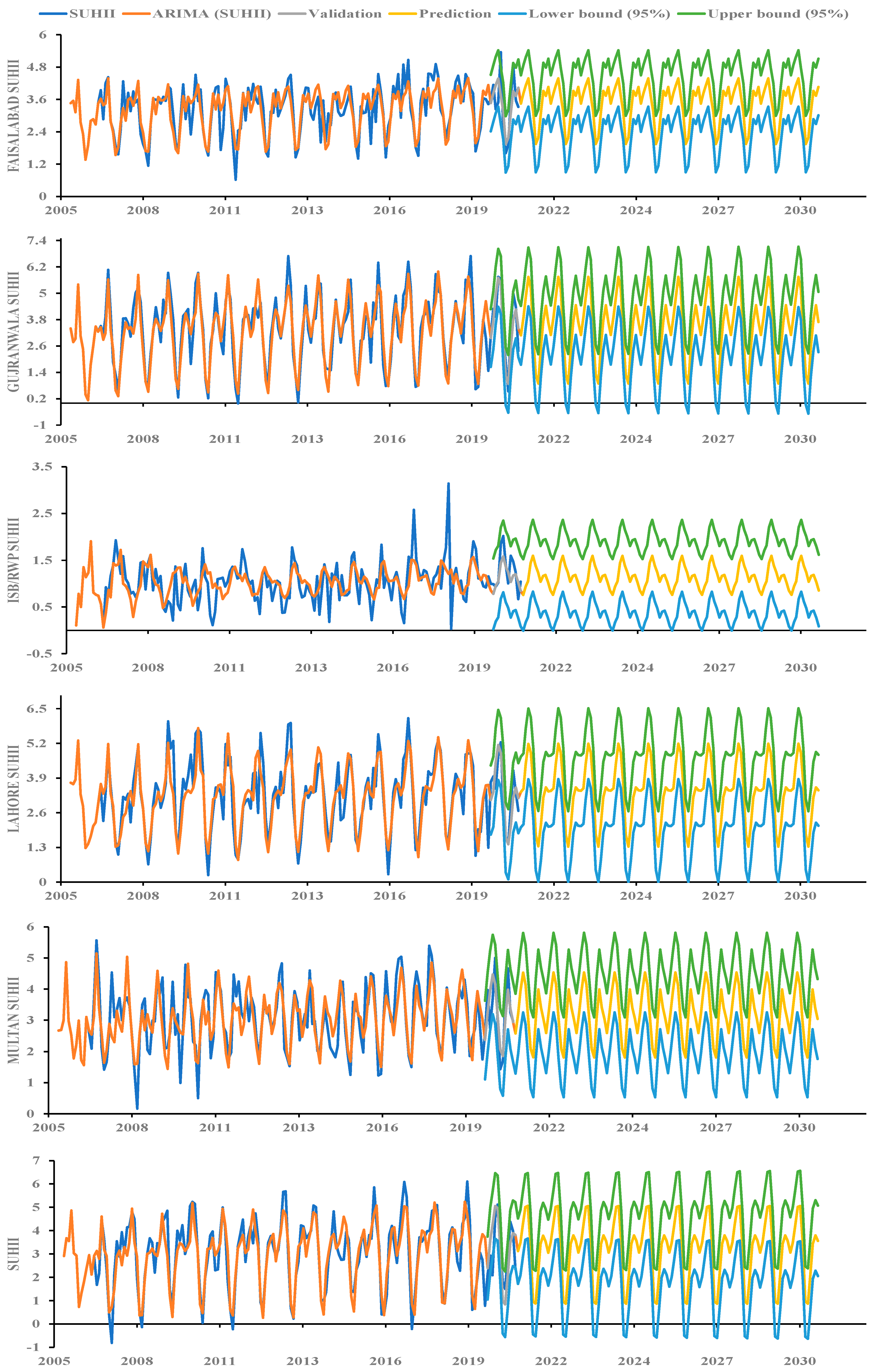
3.4. ARIMA Model for Daytime and Nighttime SUHII
4. Discussion
4.1. Implications
4.2. Limitations and Future Work
5. Conclusions
Author Contributions
Funding
Institutional Review Board Statement
Data Availability Statement
Conflicts of Interest
References
- Portela, C.I.; Massi, K.G.; Rodrigues, T.; Alcântara, E. Impact of Urban and Industrial Features on Land Surface Temperature: Evidences from Satellite Thermal Indices. Sustain. Cities Soc. 2020, 56, 102100. [Google Scholar] [CrossRef]
- Pickett, S.T.A.; Cadenasso, M.L.; Grove, J.M.; Boone, C.G.; Groffman, P.M.; Irwin, E.; Kaushal, S.S.; Marshall, V.; McGrath, B.P.; Nilon, C.H.; et al. Urban Ecological Systems: Scientific Foundations and a Decade of Progress. J. Environ. Manag. 2011, 92, 331–362. [Google Scholar] [CrossRef]
- United Nation. World Urbanization Prospects; United Nations: New York, NY, USA, 2018.
- Gong, P.; Li, X.; Wang, J.; Bai, Y.; Chen, B.; Hu, T.; Liu, X.; Xu, B.; Yang, J.; Zhang, W.; et al. Annual Maps of Global Artificial Impervious Area (GAIA) between 1985 and 2018. Remote Sens. Environ. 2020, 236, 111510. [Google Scholar] [CrossRef]
- Fitria, R.; Kim, D.; Baik, J.; Choi, M. Impact of Biophysical Mechanisms on Urban Heat Island Associated with Climate Variation and Urban Morphology. Sci. Rep. 2019, 9, 19503. [Google Scholar] [CrossRef] [PubMed] [Green Version]
- Salazar, A.; Baldi, G.; Hirota, M.; Syktus, J.; McAlpine, C. Land Use and Land Cover Change Impacts on the Regional Climate of Non-Amazonian South America: A Review. Glob. Planet. Chang. 2015, 128, 103–119. [Google Scholar] [CrossRef]
- Howard, L. The Climate of London Deduced from Meteorological Observations; Cambridge University Press: Cambridge, UK, 1833; Volume 1. [Google Scholar]
- Niu, L.; Tang, R.; Jiang, Y.; Zhou, X. Spatiotemporal Patterns and Drivers of the Surface Urban Heat Island in 36 Major Cities in China: A Comparison of Two Different Methods for Delineating Rural Areas. Sustainability 2020, 12, 478. [Google Scholar] [CrossRef] [Green Version]
- Reid, W.V. Biodiversity Hotspots. Trends Ecol. Evol. 1998, 13, 275–280. [Google Scholar] [CrossRef]
- Keppas, S.C.; Papadogiannaki, S.; Parliari, D.; Kontos, S.; Poupkou, A.; Tzoumaka, P.; Kelessis, A.; Zanis, P.; Casasanta, G.; De’donato, F.; et al. Future Climate Change Impact on Urban Heat Island in Two Mediterranean Cities Based on High-Resolution Regional Climate Simulations. Atmosphere 2021, 12, 884. [Google Scholar] [CrossRef]
- Kabano, P.; Lindley, S.; Harris, A. Evidence of Urban Heat Island Impacts on the Vegetation Growing Season Length in a Tropical City. Landsc. Urban Plan. 2021, 206, 103989. [Google Scholar] [CrossRef]
- Brandsma, T.; Wolters, D. Measurement and Statistical Modeling of the Urban Heat Island of the City of Utrecht (The Netherlands). J. Appl. Meteorol. Climatol. 2012, 51, 1046–1060. [Google Scholar] [CrossRef]
- David Sundersingh, S. Effect of Heat Islands over Urban Madras and Measures for Its Mitigation. Energy Build 1990, 15, 245–252. [Google Scholar] [CrossRef]
- Li, K.; Chen, Y.; Wang, M.; Gong, A. Spatial-Temporal Variations of Surface Urban Heat Island Intensity Induced by Different Definitions of Rural Extents in China. Sci. Total Environ. 2019, 669, 229–247. [Google Scholar] [CrossRef] [PubMed]
- Kwak, Y.; Park, C.; Deal, B. Discerning the Success of Sustainable Planning: A Comparative Analysis of Urban Heat Island Dynamics in Korean New Towns. Sustain. Cities Soc. 2020, 61, 102341. [Google Scholar] [CrossRef]
- Lafortezza, R.; Carrus, G.; Sanesi, G.; Davies, C. Benefits and Well-Being Perceived by People Visiting Green Spaces in Periods of Heat Stress. Urban For. Urban Green. 2009, 8, 97–108. [Google Scholar] [CrossRef]
- Rao, P.K. Remote Sensing of Urban Heat Islands from an Environmental Satellite. Bull. Am. Meteorol. Soc. 1972, 53, 647–648. [Google Scholar]
- Yao, R.; Cao, J.; Wang, L.; Zhang, W.; Wu, X. Urbanization e Ff Ects on Vegetation Cover in Major African Cities During. Int. J. Appl. Earth Obs. Geoinf. 2019, 75, 44–53. [Google Scholar] [CrossRef]
- Wu, X.; Wang, G.; Yao, R.; Wang, L.; Yu, D.; Gui, X. Investigating Surface Urban Heat Islands in South America Based on MODIS Data from 2003–2016. Remote Sens. 2019, 11, 1212. [Google Scholar] [CrossRef] [Green Version]
- Peng, S.; Piao, S.; Ciais, P.; Friedlingstein, P.; Ottle, C.; Bréon, F.M.; Nan, H.; Zhou, L.; Myneni, R.B. Surface Urban Heat Island Across 419 Global Big Cities. Environ. Sci. Technol. 2012, 46, 696–703. [Google Scholar] [CrossRef]
- Quan, J.; Zhan, W.; Chen, Y.; Wang, M.; Wang, J. Time Series Decomposition of Remotely Sensed Land Surface Temperature and Investigation of Trends and Seasonal Variations in Surface Urban Heat Islands. J. Geophys. Res. Atmos. 2016, 121, 2638–2657. [Google Scholar] [CrossRef]
- Oke, T.R. Canyon Geometry and the Nocturnal Urban Heat Island: Comparison of Scale Model and Field Observations. J. Climatol. 1981, 1, 237–254. [Google Scholar] [CrossRef]
- Grimmond, S. Urbanization and Global Environmental Change: Local Effects of Urban Warming. Geogr. J. 2007, 173, 83–88. [Google Scholar] [CrossRef]
- Pongrácz, R.; Bartholy, J.; Dezső, Z. Application of Remotely Sensed Thermal Information to Urban Climatology of Central European Cities. Phys. Chem. Earth Parts A/B/C 2010, 35, 95–99. [Google Scholar] [CrossRef]
- ROTH, M.; OKE, T.R.; EMERY, W.J. Satellite-Derived Urban Heat Islands from Three Coastal Cities and the Utilization of Such Data in Urban Climatology. Int. J. Remote Sens. 1989, 10, 1699–1720. [Google Scholar] [CrossRef]
- Zhou, D.; Zhao, S.; Liu, S.; Zhang, L.; Zhu, C. Surface Urban Heat Island in China’s 32 Major Cities: Spatial Patterns and Drivers. Remote Sens. Environ. 2014, 152, 51–61. [Google Scholar] [CrossRef]
- Yao, R.; Wang, L.; Huang, X.; Niu, Z.; Liu, F.; Wang, Q. Temporal Trends of Surface Urban Heat Islands and Associated Determinants in Major Chinese Cities. Sci. Total Environ. 2017, 609, 742–754. [Google Scholar] [CrossRef]
- Tran, H.; Uchihama, D.; Ochi, S.; Yasuoka, Y. Assessment with Satellite Data of the Urban Heat Island Effects in Asian Mega Cities. Int. J. Appl. Earth Obs. Geoinf. 2006, 8, 34–48. [Google Scholar] [CrossRef]
- Chun, B.; Guldmann, J.M. Spatial Statistical Analysis and Simulation of the Urban Heat Island in High-Density Central Cities. Landsc. Urban Plan. 2014, 125, 76–88. [Google Scholar] [CrossRef]
- Su, Y.F.; Foody, G.M.; Cheng, K.S. Spatial Non-Stationarity in the Relationships between Land Cover and Surface Temperature in an Urban Heat Island and Its Impacts on Thermally Sensitive Populations. Landsc. Urban Plan. 2012, 107, 172–180. [Google Scholar] [CrossRef]
- Oh, J.W.; Ngarambe, J.; Duhirwe, P.N.; Yun, G.Y.; Santamouris, M. Using Deep-Learning to Forecast the Magnitude and Characteristics of Urban Heat Island in Seoul Korea. Sci. Rep. 2020, 10, 3559. [Google Scholar] [CrossRef] [Green Version]
- Wang, J.; Pauleit, S.; Banzhaf, E. An Integrated Indicator Framework for the Assessment of Multifunctional Green Infrastructure—Exemplified in a European City. Remote Sens. 2019, 11, 1869. [Google Scholar] [CrossRef] [Green Version]
- Ustaoglu, B.; Cigizoglu, H.K.; Karaca, M. Forecast of Daily Mean, Maximum and Minimum Temperature Time Series by Three Artificial Neural Network Methods. Meteorol. Appl. 2008, 15, 431–445. [Google Scholar] [CrossRef]
- Imhoff, M.L.; Zhang, P.; Wolfe, R.E.; Bounoua, L. Remote Sensing of the Urban Heat Island Effect across Biomes in the Continental USA. Remote Sens. Environ. 2010, 114, 504–513. [Google Scholar] [CrossRef] [Green Version]
- Schatz, J.; Kucharik, C.J. Seasonality of the Urban Heat Island Effect in Madison, Wisconsin. J. Appl. Meteorol. Climatol. 2014, 53, 2371–2386. [Google Scholar] [CrossRef]
- Zhou, B.; Rybski, D.; Kropp, J.P. On the Statistics of Urban Heat Island Intensity. Geophys. Res. Lett. 2013, 40, 5486–5491. [Google Scholar] [CrossRef]
- Zhou, D.; Zhao, S.; Liu, S.; Zhang, L. Spatiotemporal Trends of Terrestrial Vegetation Activity along the Urban Development Intensity Gradient in China’s 32 Major Cities. Sci. Total Environ. 2014, 488–489, 136–145. [Google Scholar] [CrossRef] [PubMed]
- Wang, J.; Huang, B.; Fu, D.; Atkinson, P.M. Spatiotemporal Variation in Surface Urban Heat Island Intensity and Associated Determinants across Major Chinese Cities. Remote Sens. 2015, 7, 3670–3689. [Google Scholar] [CrossRef] [Green Version]
- Meng, Q.; Zhang, L.; Sun, Z.; Meng, F.; Wang, L.; Sun, Y. Characterizing Spatial and Temporal Trends of Surface Urban Heat Island Effect in an Urban Main Built-up Area: A 12-Year Case Study in Beijing, China. Remote Sens. Environ. 2018, 204, 826–837. [Google Scholar] [CrossRef]
- Peng, J.; Ma, J.; Liu, Q.; Liu, Y.; Hu, Y.; Li, Y.; Yue, Y. Spatial-Temporal Change of Land Surface Temperature across 285 Cities in China: An Urban-Rural Contrast Perspective. Sci. Total Environ. 2018, 635, 487–497. [Google Scholar] [CrossRef]
- Siddique, M.A.; Dongyun, L.; Li, P.; Rasool, U.; Khan, T.U.; Farooqi, T.J.A.; Wang, L.; Fan, B.; Rasool, M.A. Assessment and Simulation of Land Use and Land Cover Change Impacts on the Land Surface Temperature of Chaoyang District in Beijing, China. PeerJ 2020, 2020, e9115. [Google Scholar] [CrossRef]
- Akinyemi, F.O.; Ikanyeng, M.; Muro, J. Land Cover Change Effects on Land Surface Temperature Trends in an African Urbanizing Dryland Region. City Environ. Interact. 2019, 4, 100029. [Google Scholar] [CrossRef]
- Yao, R.; Wang, L.; Huang, X.; Zhang, W.; Li, J.; Niu, Z. Interannual Variations in Surface Urban Heat Island Intensity and Associated Drivers in China. J. Environ. Manag. 2018, 222, 86–94. [Google Scholar] [CrossRef] [PubMed]
- Zhou, D.; Zhang, L.; Hao, L.; Sun, G.; Liu, Y.; Zhu, C. Spatiotemporal Trends of Urban Heat Island Effect along the Urban Development Intensity Gradient in China. Sci. Total Environ. 2016, 544, 617–626. [Google Scholar] [CrossRef] [PubMed]
- Yao, R.; Wang, L.; Gui, X.; Zheng, Y.; Zhang, H.; Huang, X. Urbanization Effects on Vegetation and Surface Urban Heat Islands in China ’ s Yangtze River Basin. Remote Sens. 2017, 9, 540. [Google Scholar] [CrossRef] [Green Version]
- Khan, M.S.; Ullah, S.; Chen, L. Comparison on Land-Use/Land-Cover Indices in Explaining Land Surface Temperature Variations in the City of Beijing, China. Land 2021, 10, 1018. [Google Scholar] [CrossRef]
- Yao, R.; Wang, L.; Huang, X.; Liu, Y.; Niu, Z.; Wang, S.; Wang, L. Long-Term Trends of Surface and Canopy Layer Urban Heat Island Intensity in 272 Cities in the Mainland of China. Sci. Total Environ. 2021, 772, 145607. [Google Scholar] [CrossRef]
- Barat, A.; Kumar, S.; Kumar, P.; Parth Sarthi, P. Characteristics of Surface Urban Heat Island (SUHI) over the Gangetic Plain of Bihar, India. Asia-Pac. J. Atmos. Sci. 2018, 54, 205–214. [Google Scholar] [CrossRef]
- Ranagalage, M.; Estoque, R.C.; Zhang, X.; Murayama, Y. Spatial Changes of Urban Heat Island Formation in the Colombo District, Sri Lanka: Implications for Sustainability Planning. Sustainability 2018, 10, 1367. [Google Scholar] [CrossRef] [Green Version]
- Dissanayake, D.; Morimoto, T.; Murayama, Y.; Ranagalage, M.; Handayani, H.H. Impact of Urban Surface Characteristics and Socio-Economic Variables on the Spatial Variation of Land Surface Temperature in Lagos City, Nigeria. Sustainability 2018, 11, 25. [Google Scholar] [CrossRef] [Green Version]
- Rousta, I.; Sarif, M.O.; Gupta, R.D.; Olafsson, H.; Ranagalage, M.; Murayama, Y.; Zhang, H.; Mushore, T.D. Spatiotemporal Analysis of Land Use/Land Cover and Its Effects on Surface Urban Heat Island Using Landsat Data: A Case Study of Metropolitan City Tehran (1988–2018). Sustainability 2018, 10, 4433. [Google Scholar] [CrossRef] [Green Version]
- Khan, M.S.; Ullah, S.; Sun, T.; Rehman, A.U.; Chen, L. Land-Use/Land-Cover Changes and Its Contribution to Urban Heat Island: A Case Study of Islamabad, Pakistan. Sustainability 2020, 12, 3861. [Google Scholar] [CrossRef]
- Rehman, A.; Qin, J.; Shafi, S.; Khan, M.S.; Ullah, S.; Ahmad, K.; Rehman, N.U.; Faheem, M. Modelling of Land Use/Cover and LST Variations by Using GIS and Remote Sensing: A Case Study of the Northern Pakhtunkhwa Mountainous Region, Pakistan. Sensors 2022, 22, 4965. [Google Scholar] [CrossRef] [PubMed]
- Rizvi, S.H.; Fatima, H.; Alam, K.; Iqbal, M.J. The Surface Urban Heat Island Intensity and Urban Expansion: A Comparative Analysis for the Coastal Areas of Pakistan. Environ. Dev. Sustain. 2021, 23, 5520–5537. [Google Scholar] [CrossRef]
- Imran, M.; Mehmood, A. Analysis and Mapping of Present and Future Drivers of Local Urban Climate Using Remote Sensing: A Case of Lahore, Pakistan. Arab. J. Geosci. 2020, 13, 278. [Google Scholar] [CrossRef]
- Aslam, B.; Maqsoom, A.; Khalid, N.; Ullah, F.; Sepasgozar, S. Urban Overheating Assessment through Prediction of Surface Temperatures: A Case Study of Karachi, Pakistan. ISPRS Int. J. Geoinf. 2021, 10, 539. [Google Scholar] [CrossRef]
- Government of Pakistan. 2017 Provincial Census Report; Pakistan Bureau of Statistics, Government of Pakistan: Islamabad, Pakistan, 2017.
- Benas, N.; Chrysoulakis, N.; Cartalis, C. Trends of Urban Surface Temperature and Heat Island Characteristics in the Mediterranean. Theor Appl Climatol 2017, 130, 807–816. [Google Scholar] [CrossRef]
- Dilawar, A.; Chen, B.; Trisurat, Y.; Tuankrua, V.; Arshad, A.; Hussain, Y.; Measho, S.; Guo, L.; Kayiranga, A.; Zhang, H.; et al. Spatiotemporal Shifts in Thermal Climate in Responses to Urban Cover Changes: A-Case Analysis of Major Cities in Punjab, Pakistan. Geomat. Nat. Hazards Risk 2021, 12, 763–793. [Google Scholar] [CrossRef]
- Samie, A.; Abbas, A.; Azeem, M.M.; Hamid, S.; Iqbal, M.A.; Hasan, S.S.; Deng, X. Examining the Impacts of Future Land Use/Land Cover Changes on Climate in Punjab Province, Pakistan: Implications for Environmental Sustainability and Economic Growth. Environ. Sci. Pollut. Res. 2020, 27, 25415–25433. [Google Scholar] [CrossRef]
- Hijmans, R.J.; Cameron, S.E.; Parra, J.L.; Jones, P.G.; Jarvis, A. Very High Resolution Interpolated Climate Surfaces for Global Land Areas. Int. J. Climatol. 2005, 25, 1965–1978. [Google Scholar] [CrossRef]
- Siddiqui, A.; Kushwaha, G.; Nikam, B.; Srivastav, S.K.; Shelar, A.; Kumar, P. Analysing the Day/Night Seasonal and Annual Changes and Trends in Land Surface Temperature and Surface Urban Heat Island Intensity (SUHII) for Indian Cities. Sustain. Cities Soc. 2021, 75, 103374. [Google Scholar] [CrossRef]
- Yao, N.; Huang, C.; Yang, J.; van den Bosch, C.C.K.; Ma, L.; Jia, Z. Combined Effects of Impervious Surface Change and Large-Scale Afforestation on the Surface Urban Heat Island Intensity of Beijing, China Based on Remote Sensing Analysis. Remote Sens. 2020, 12, 3906. [Google Scholar] [CrossRef]
- Chen, C.; Li, D.; Keenan, T.F. Enhanced Surface Urban Heat Islands Due to Divergent Urban-Rural Greening Trends. Environ. Res. Lett. 2021, 16, 124071. [Google Scholar] [CrossRef]
- Wang, Y.; Luo, Y.; Tan, W.; Su, H. Analysis of Temporal and Spatial Variation Process of Dianchi Lake Surface Water Temperature Based on MODIS Remote Sensing Images. IOP Conf. Ser. Earth Environ. Sci. 2021, 658, 012005. [Google Scholar] [CrossRef]
- Bala, R.; Yadav, V.P.; Prasad, R. Seasonal Variation of Day and Night Land Surface Temperature with Normalized Difference Vegetation Index Using MODIS Satellite Imagery. In Proceedings of the 2020 URSI Regional Conference on Radio Science (URSI-RCRS), Varanasi, India, 12–14 February 2020; pp. 1–4. [Google Scholar]
- Zafar, Z.; Mehmood, M.S.; Ahamad, M.I.; Chudhary, A.; Abbas, N.; khan, A.R.; Zulqarnain, R.M.; Abdal, S. Trend Analysis of the Decadal Variations of Water Bodies and Land Use/Land Cover through MODIS Imagery: An in-Depth Study from Gilgit-Baltistan, Pakistan. Water Supply 2020, 21, 927–940. [Google Scholar] [CrossRef]
- Yao, R.; Wang, L.; Huang, X.; Niu, Y.; Chen, Y.; Niu, Z. The Influence of Different Data and Method on Estimating the Surface Urban Heat Island Intensity. Ecol. Indic. 2018, 89, 45–55. [Google Scholar] [CrossRef]
- Sun, R.; Lü, Y.; Yang, X.; Chen, L. Understanding the Variability of Urban Heat Islands from Local Background Climate and Urbanization. J Clean Prod 2019, 208, 743–752. [Google Scholar] [CrossRef]
- Wang, Z.; Liu, M.; Liu, X.; Meng, Y.; Zhu, L.; Rong, Y. Spatio-Temporal Evolution of Surface Urban Heat Islands in the Chang-Zhu-Tan Urban Agglomeration. Phys. Chem. Earth Parts A/B/C 2020, 117, 102865. [Google Scholar] [CrossRef]
- Gocic, M.; Trajkovic, S. Analysis of Changes in Meteorological Variables Using Mann-Kendall and Sen’s Slope Estimator Statistical Tests in Serbia. Glob. Planet. Chang. 2013, 100, 172–182. [Google Scholar] [CrossRef]
- Mann, H.B. Nonparametric Tests against Trend. Econometrica 1945, 13, 259. [Google Scholar] [CrossRef]
- Mahmood, R.; Jia, S.; Zhu, W. Analysis of Climate Variability, Trends, and Prediction in the Most Active Parts of the Lake Chad Basin, Africa. Sci. Rep. 2019, 9, 6317. [Google Scholar] [CrossRef] [Green Version]
- Bilal, H. Recent Snow Cover Variation in the Upper Indus Basin of Gilgit Baltistan, Hindukush Karakoram Himalaya. J. Mt. Sci. 2019, 16, 296–308. [Google Scholar] [CrossRef]
- Chattopadhyay, G.; Chakraborthy, P.; Chattopadhyay, S. Mann–Kendall Trend Analysis of Tropospheric Ozone and Its Modeling Using ARIMA. Theor. Appl. Climatol. 2012, 110, 321–328. [Google Scholar] [CrossRef]
- Sen, P.K. Estimates of the Regression Coefficient Based on Kendall’s Tau. J. Am. Stat. Assoc. 1968, 63, 1379–1389. [Google Scholar] [CrossRef]
- Atta-ur-Rahman; Dawood, M. Spatio-Statistical Analysis of Temperature Fluctuation Using Mann-Kendall and Sen’s Slope Approach. Clim. Dyn. 2017, 48, 783–797. [Google Scholar] [CrossRef]
- Cryer, J.D.; Chan, K.-S. Springer Texts in Statistics Time Series Analysis: With Applications in R, 2nd ed.; Springer: Berlin/Heidelberg, Germany, 2008. [Google Scholar]
- Wang, H.R.; Wang, C.; Lin, X.; Kang, J. An Improved ARIMA Model for Precipitation Simulations. Nonlin. Process. Geophys. 2014, 21, 1159–1168. [Google Scholar] [CrossRef] [Green Version]
- al Sayah, M.J.; Abdallah, C.; Khouri, M.; Nedjai, R.; Darwich, T. A Framework for Climate Change Assessment in Mediterranean Data-Sparse Watersheds Using Remote Sensing and ARIMA Modeling. Theor. Appl. Climatol. 2021, 143, 639–658. [Google Scholar] [CrossRef]
- Kwiatkowski, D.; Phillips, P.C.B.; Schmidt, P.; Shin, Y. Testing the Null Hypothesis of Stationarity against the Alternative of a Unit Root: How Sure Are We That Economic Time Series Have a Unit Root? J. Econom. 1992, 54, 159–178. [Google Scholar] [CrossRef]
- Adhikari, R.; Agrawal, R. An Introductory Study on Time Series Modeling and Forecasting; Lambert Academic Publishing: London, UK, 2013; ISBN 978-3-659-33508-2. [Google Scholar]
- Breitung, J.; Pesaran, M.H. Unit Roots and Cointegration in Panels. In The Econometrics of Panel Data: Fundamentals and Recent Developments in Theory and Practice; Mátyás, L., Sevestre, P., Eds.; Springer: Berlin/Heidelberg, Germany, 2008; pp. 279–322. ISBN 978-3-540-75892-1. [Google Scholar]
- Zhang, X.; Zhang, L.; Zhang, Y.; Liao, Z.; Song, J. Predicting Trend of Early Childhood Caries in Mainland China: A Combined Meta-Analytic and Mathematical Modelling Approach Based on Epidemiological Surveys. Sci. Rep. 2017, 7, 6507. [Google Scholar] [CrossRef] [Green Version]
- Arshad, S.; Ahmad, S.R.; Abbas, S.; Asharf, A.; Siddiqui, N.A.; ul Islam, Z. Quantifying the Contribution of Diminishing Green Spaces and Urban Sprawl to Urban Heat Island Effect in a Rapidly Urbanizing Metropolitan City of Pakistan. Land Use Policy 2022, 113, 105874. [Google Scholar] [CrossRef]
- AlDousari, A.E.; al Kafy, A.; Saha, M.; Fattah, M.A.; Almulhim, A.I.; al Faisal, A.; al Rakib, A.; Jahir, D.M.A.; Rahaman, Z.A.; Bakshi, A.; et al. Modelling the Impacts of Land Use/Land Cover Changing Pattern on Urban Thermal Characteristics in Kuwait. Sustain. Cities Soc. 2022, 86, 104107. [Google Scholar] [CrossRef]
- Rahaman, Z.A.; Kafy, A.-A.; Saha, M.; Rahim, A.A.; Almulhim, A.I.; Rahaman, S.N.; Fattah, M.A.; Rahman, M.T.; S, K.; Al Faisal, A.; et al. Assessing the Impacts of Vegetation Cover Loss on Surface Temperature, Urban Heat Island and Carbon Emission in Penang City, Malaysia. Build. Environ. 2022, 222, 109335. [Google Scholar] [CrossRef]
- al Kafy, A.; Rahman, M.S.; al Faisal, A.; Hasan, M.M.; Islam, M. Modelling Future Land Use Land Cover Changes and Their Impacts on Land Surface Temperatures in Rajshahi, Bangladesh. Remote Sens. Appl. 2020, 18, 100314. [Google Scholar] [CrossRef]
- al Faisal, A.; Kafy, A.A.; al Rakib, A.; Akter, K.S.; Jahir, D.M.A.; Sikdar, M.S.; Ashrafi, T.J.; Mallik, S.; Rahman, M.M. Assessing and Predicting Land Use/Land Cover, Land Surface Temperature and Urban Thermal Field Variance Index Using Landsat Imagery for Dhaka Metropolitan Area. Environ. Chall. 2021, 4, 100192. [Google Scholar] [CrossRef]
- Naim, M.N.H.; Kafy, A.A. Assessment of Urban Thermal Field Variance Index and Defining the Relationship between Land Cover and Surface Temperature in Chattogram City: A Remote Sensing and Statistical Approach. Environ. Chall. 2021, 4, 100107. [Google Scholar] [CrossRef]
- al Kafy, A.; al Faisal, A.; Rahman, M.S.; Islam, M.; al Rakib, A.; Islam, M.A.; Khan, M.H.H.; Sikdar, M.S.; Sarker, M.H.S.; Mawa, J.; et al. Prediction of Seasonal Urban Thermal Field Variance Index Using Machine Learning Algorithms in Cumilla, Bangladesh. Sustain. Cities Soc. 2021, 64, 102542. [Google Scholar] [CrossRef]
- Saha, M.; al Kafy, A.; Bakshi, A.; al Faisal, A.; Almulhim, A.I.; Rahaman, Z.A.; al Rakib, A.; Fattah, M.A.; Akter, K.S.; Rahman, M.T.; et al. Modelling Microscale Impacts Assessment of Urban Expansion on Seasonal Surface Urban Heat Island Intensity Using Neural Network Algorithms. Energy Build. 2022, 275, 112452. [Google Scholar] [CrossRef]
- Zhang, M.; Zhang, C.; al Kafy, A.; Tan, S. Simulating the Relationship between Land Use/Cover Change and Urban Thermal Environment Using Machine Learning Algorithms in Wuhan City, China. Land 2022, 11, 14. [Google Scholar] [CrossRef]
- Phelan, P.E.; Kaloush, K.; Miner, M.; Golden, J.; Phelan, B.; Silva, H.; Taylor, R.A. Urban Heat Island: Mechanisms, Implications, and Possible Remedies. Annu. Rev. Environ. Resour. 2015, 40, 285–307. [Google Scholar] [CrossRef]
- Wang, C.; Myint, S.W.; Wang, Z.; Song, J. Spatio-Temporal Modeling of the Urban Heat Island in the Phoenix Metropolitan Area: Land Use Change Implications. Remote Sens. 2016, 8, 185. [Google Scholar] [CrossRef] [Green Version]
- Akbari, H.; Cartalis, C.; Kolokotsa, D.; Muscio, A.; Pisello, A.L.; Rossi, F.; Santamouris, M.; Synnefa, A.; Wong, N.H.; Zinzi, M. Local Climate Change and Urban Heat Island Mitigation Techniques—The State of the Art. J. Civ. Eng. Manag. 2016, 22, 1–16. [Google Scholar] [CrossRef] [Green Version]
- Shen, H.; Meng, X.; Zhang, L. An Integrated Framework for the Spatio-Temporal-Spectral Fusion of Remote Sensing Images. IEEE Trans. Geosci. Remote Sens. 2016, 54, 7135–7148. [Google Scholar] [CrossRef]
- Zeng, C.; Shen, H.; Zhang, L. Recovering Missing Pixels for Landsat ETM+ SLC-off Imagery Using Multi-Temporal Regression Analysis and a Regularization Method. Remote Sens. Environ. 2013, 131, 182–194. [Google Scholar] [CrossRef]


| City Name | Total Area (km2) | Total Population | Urban Percentage | Population Density (km−2) |
|---|---|---|---|---|
| Lahore | 1772 | 11,119,985 | 100 | 6275.39 |
| Faisalabad | 5857 | 7,882,444 | 47.79 | 1345.82 |
| ISB/RWP | 6191 | 7,405,748 | 53.00 | 1616.715 |
| Gujranwala | 3622 | 5,011,066 | 58.85 | 1383.51 |
| Multan | 3720 | 4,746,166 | 43.38 | 1275.85 |
| Sialkot | 3016 | 3,894,938 | 29.39 | 1291.43 |
| City | Daytime SUHII (°C) | Nighttime SUHII (°C) | ||||||||
|---|---|---|---|---|---|---|---|---|---|---|
| Annual | Winter | Spring | Summer | Autumn | Annual | Winter | Spring | Summer | Autumn | |
| Lahore | 2.924 | 1.837 | 3.902 | 3.542 | 2.393 | 3.232 | 3.382 | 4.639 | 2.078 | 2.841 |
| Faisalabad | 3.139 | 1.609 | 3.915 | 3.854 | 3.147 | 3.213 | 3.540 | 3.809 | 2.139 | 3.377 |
| ISB/RWP | −0.219 | −0.923 | −0.160 | 0.582 | −0.416 | 1.042 | 0.750 | 1.268 | 1.121 | 1.024 |
| Gujranwala | 2.108 | 0.717 | 2.324 | 2.266 | 3.071 | 3.336 | 3.436 | 4.980 | 1.514 | 3.449 |
| Multan | 3.327 | 1.823 | 3.947 | 4.118 | 3.417 | 3.069 | 2.822 | 4.007 | 2.102 | 3.357 |
| Sialkot | 2.045 | 0.065 | 2.017 | 2.944 | 3.146 | 3.045 | 3.269 | 4.425 | 1.542 | 2.982 |
| Average | 2.221 | 0.855 | 2.657 | 2.877 | 2.460 | 2.823 | 2.866 | 3.855 | 1.749 | 2.838 |
| City | Daytime SUHII (°C) | Nighttime SUHII (°C) | ||
|---|---|---|---|---|
| Mean | SD | Mean | SD | |
| Lahore | 2.924 | 1.289 | 3.229 | 1.288 |
| Faisalabad | 3.139 | 1.304 | 3.214 | 0.916 |
| ISB/RWP | −0.219 | 1.295 | 1.042 | 0.452 |
| Gujranwala | 2.108 | 2.476 | 3.332 | 1.541 |
| Multan | 3.327 | 1.633 | 3.068 | 1.023 |
| Sialkot | 2.045 | 2.154 | 3.041 | 1.427 |
| Average | 2.221 | 1.370 | 2.821 | 0.975 |
| City | Daytime SUHII (° C/Year) | Nighttime SUHII (°C/Year) | |||||||||
|---|---|---|---|---|---|---|---|---|---|---|---|
| Annual | Winter | Spring | Summer | Autumn | Annual | Winter | Spring | Summer | Autumn | ||
| Lahore | Z | 0.048 | 0.029 | 0.219 | −0.105 | −0.448 * | 0.295 | 0.048 | 0.162 | 0.181 | 0.371 * |
| S | 0.002 | 0.007 | 0.041 | −0.016 | −0.040 | 0.032 | 0.016 | 0.036 | 0.028 | 0.050 | |
| Faisalabad | Z | 0.124 | 0.333 | 0.124 | 0.067 | 0.124 | 0.543 ** | 0.181 | 0.390 * | 0.371 * | 0.486 |
| S | 0.016 | 0.056 | 0.023 | 0.008 | 0.007 | 0.039 | 0.037 | 0.039 | 0.039 | 0.034 | |
| ISB/RWP | Z | 0.581 ** | 0.314 | 0.543 ** | 0.410 * | 0.562 ** | 0.486 * | 0.219 | 0.333 | 0.162 | 0.314 |
| S | 0.095 | 0.037 | 0.178 | 0.114 | 0.092 | 0.025 | 0.016 | 0.034 | 0.013 | 0.017 | |
| Gujranwala | Z | 0.276 | −0.124 | 0.295 | 0.124 | 0.124 | 0.314 | −0.048 | 0.390 * | 0.371 * | 0.314 |
| S | 0.031 | −0.015 | 0.057 | 0.042 | 0.015 | 0.030 | −0.003 | 0.077 | 0.036 | 0.049 | |
| Multan | Z | −0.105 | 0.200 | 0.086 | −0.219 | −0.371 * | 0.314 | 0.067 | 0.143 | 0.162 | 0.352 * |
| S | −0.014 | 0.054 | 0.016 | −0.060 | −0.094 | 0.025 | 0.008 | 0.024 | 0.023 | 0.042 | |
| Sialkot | Z | 0.371 * | 0.371 * | 0.257 | 0.314 | −0.086 | 0.333 * | −0.067 | 0.257 | 0.333 | 0.371 * |
| S | 0.040 | 0.062 | 0.054 | 0.063 | −0.006 | 0.030 | −0.021 | 0.073 | 0.056 | 0.041 | |
| Average | Z | 0.410 * | 0.448 * | 0.486 * | 0.276 | 0.086 | 0.485 * | 0.067 | 0.314 | 0.352 * | 0.390 * |
| S | 0.031 | 0.036 | 0.061 | 0.027 | 0.006 | 0.032 | 0.006 | 0.043 | 0.029 | 0.034 | |
| City | Daytime SUHII (°C) | Nighttime SUHII (°C) | ||||
|---|---|---|---|---|---|---|
| p-Value (ADF) | RMSE | MAPE | p-Value (ADF) | RMSE | MAPE | |
| Lahore | <0.0001 | 0.74 | 0.24 | <0.0001 | 0.66 | 0.19 |
| Faisalabad | <0.0001 | 0.77 | 0.3 | <0.0001 | 0.53 | 0.14 |
| ISB/RWP | <0.0001 | 0.75 | 2.19 | <0.0001 | 0.38 | 0.63 |
| Gujranwala | <0.0001 | 0.82 | 0.76 | <0.0001 | 0.66 | 0.56 |
| Multan | <0.0001 | 1 | 0.46 | <0.0001 | 0.64 | 0.22 |
| Sialkot | <0.0001 | 0.91 | 1.39 | <0.0001 | 0.68 | 0.32 |
| Average | <0.0001 | 0.43 | 2.98 | <0.0001 | 0.43 | 0.12 |
Disclaimer/Publisher’s Note: The statements, opinions and data contained in all publications are solely those of the individual author(s) and contributor(s) and not of MDPI and/or the editor(s). MDPI and/or the editor(s) disclaim responsibility for any injury to people or property resulting from any ideas, methods, instructions or products referred to in the content. |
© 2022 by the authors. Licensee MDPI, Basel, Switzerland. This article is an open access article distributed under the terms and conditions of the Creative Commons Attribution (CC BY) license (https://creativecommons.org/licenses/by/4.0/).
Share and Cite
Mehmood, M.S.; Zafar, Z.; Sajjad, M.; Hussain, S.; Zhai, S.; Qin, Y. Time Series Analyses and Forecasting of Surface Urban Heat Island Intensity Using ARIMA Model in Punjab, Pakistan. Land 2023, 12, 142. https://doi.org/10.3390/land12010142
Mehmood MS, Zafar Z, Sajjad M, Hussain S, Zhai S, Qin Y. Time Series Analyses and Forecasting of Surface Urban Heat Island Intensity Using ARIMA Model in Punjab, Pakistan. Land. 2023; 12(1):142. https://doi.org/10.3390/land12010142
Chicago/Turabian StyleMehmood, Muhammad Sajid, Zeeshan Zafar, Muhammad Sajjad, Sadam Hussain, Shiyan Zhai, and Yaochen Qin. 2023. "Time Series Analyses and Forecasting of Surface Urban Heat Island Intensity Using ARIMA Model in Punjab, Pakistan" Land 12, no. 1: 142. https://doi.org/10.3390/land12010142