1. Introduction
The presence and use of viewshed analyses in landscape assessment have existed for decades (see [
1,
2,
3,
4] for examples and history). A variety of research on the use, optimization, and limitations of viewsheds was conducted in the 1990s [
5,
6,
7]. In the past couple of decades, there has been a surge in extending the traditional binary viewshed to more nuanced forms and applications including the assessment of oceanic blue space [
8], visualscape [
9], visual exposure [
10], cumulative viewsheds, the identification of key archaeological elements [
11], and identifying the impacts to housing prices from wind-energy infrastructure [
12].
There have also been significant efforts to optimize viewsheds in a geographic information system to improve the reliability of the analysis, the sampling techniques, and the speed with which the analysis is completed. For instance, [
13] used a simulated annealing technique to identify the optimal locations at which to generate viewsheds in order to maximize the visible area using laser scans. Earlier, [
14,
15] both developed optimal approaches to viewsheds using graphics-processing units (GPUs) with dramatic improvements over CPU-based algorithms. Additional prior work was developed to show how to more efficiently calculate a viewshed that gave rise to several of these new optimal variations [
16].
Approaches to improve efficiency can greatly reduce the amount of time it takes to render a specific analysis. However, reducing the time it takes to conduct the analysis is only one part of the equation; the other is selecting which viewpoints should be a part of the analysis. Within the literature, there seems to be less of a focus on selecting optimal and appropriate viewpoints for landscape planning; instead, there tends to be a focus on either the optimal number of viewpoints for a large area for maximum coverage or on selecting representative key observation points (KOPs). It can be useful to note that the literature and guidebooks use terms such as viewpoints, vantage points, and KOPs to represent locations from which an observer looks out toward space. There are subtleties and histories behind these terms, but in this paper, we used the term viewpoint to represent the location of an observation point. For instance, a technique for reducing the number of viewpoints for the maximum coverage over an entire area (total viewshed), assuming that peaks are the ideal viewpoints for maximum coverage, has been developed [
17]. Likewise, a similar approach toward applications where the total viewshed is the key issue continues to be developed [
18]. However, there is limited research on systematic techniques, particularly those assessed with empirical data that identify how to select optimal key observation points, with a recent exception that addresses this shortfall [
19]. These limitations are compounded because a singular KOP may not be adequate for representing landscapes that are experienced as a journey (route-based) rather than over-representing singular observation points [
20].
Visual impact assessments are often underpinned by a viewshed-analysis tool, which is commonly used by landscape planners and landscape architects [
19,
21,
22]. Typically, the outcome is a rudimentary binary result that merely identifies if a space on the surface of the earth is visible or not (ESRI ArcPro [
23] is the primary software used in industry and the viewshed is binary or cumulative [
20]). When this tool is combined with KOPs, the result is a story that merely showcases where impacts might be visible, which is not effective in assessing the degree of the impact. To compare the degree of the impact, one needs to use a tool that offers a meaningful assessment beyond the binary approach [
24]. For instance, the assessment of visualscapes [
9], visual exposure [
10], and cumulative viewsheds [
25] offer some form of continuous value for the assessment, while other advanced viewsheds can provide a visual horizon [
26]. One of the original visual analysis methods used in landscape planning is called visual magnitude [
27].
Visual magnitude has been adapted in several iterations, but these have resulted in stand-alone scripts that are not readily accessed via download or easy to implement [
20,
28]. Recently, new efforts introduced an ESRI ArcPro plugin used for a visual-magnitude analysis [
29]. This analysis has been recently named the Geospatial Route Analysis and Visual Impact Assessment (GRAVIA) tool [
30]. GRAVIA is created from the measurements of slope, aspect, distance, and the number of times seen, with the potential to analyze a range of potential infrastructural changes on the landscape (e.g., wind turbines, natural-gas infrastructure, mining activities). GRAVIA offers a means to systematically evaluate how different viewpoint-sampling distributions along a route can influence the visibility as a degree of magnitude, instead of a simple binary outcome.
The inspiration for this paper stems from the lack of empirical work conducted on viewshed analysis and viewpoint optimization for landscape planning, with a particular focus on the identification of route-based experiences where experiences of the landscape are nuanced by the topography and the distance of viewing that topography. To address these shortfalls, we asked three key research questions: (1) What is the trade-off between the number of sample points and the accuracy of the visual-magnitude model? (2) Further, can we identify an optimal trade-off between the number of viewpoints needed to represent an experience and the accuracy of the visual-magnitude analysis? (3) How does the distance from the route impact the calculations across our three environments? To answer these questions, we developed a systematic approach toward analyzing visual-magnitude models using GRAVIA in three distinct landscapes using various sampling techniques, with the results highlighting the differences and errors between the sampling techniques. To answer these questions, three objectives were created: (1) develop a repeatable process that can be validated further by other researchers, (2) assess the effectiveness of a random versus interval viewpoint-sampling technique, and (3) compare the outcomes of three different landscape typologies (i.e., mountains, hills, and flat landscapes). We note that this paper is a significant expansion of a version published earlier in a proceedings paper [
31].
2. Materials and Methods
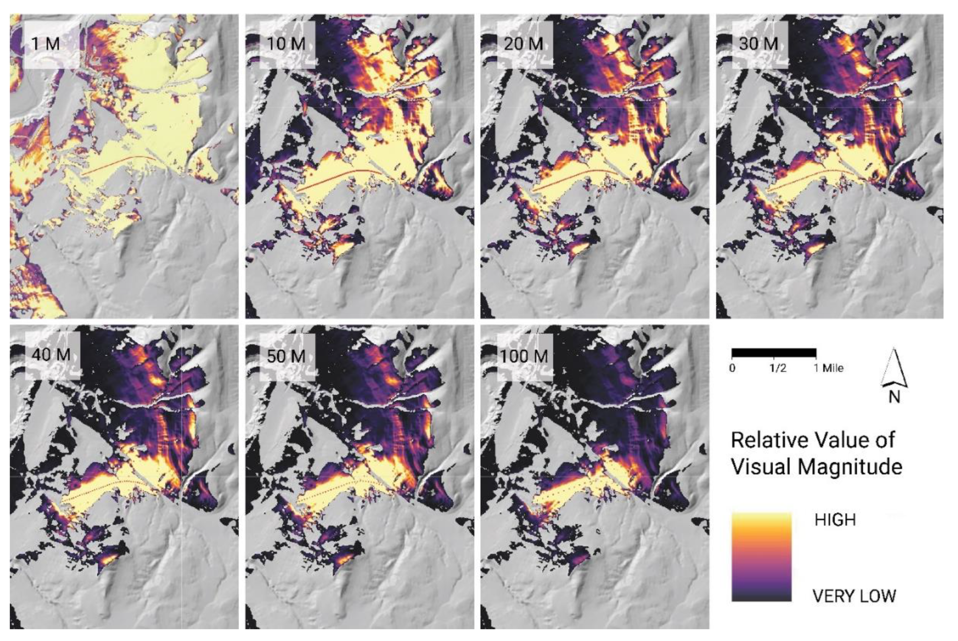
Figure 1 gives an overview of the process we used to conduct this study. This process was utilized for all terrain types, as well as both viewpoint-reduction methods. The process included the following steps: (1) data collection, (2) site and route selection, (3) the creation of viewpoint measures of 1, 10, 20, 30, 40, 50, and 100 m for each environment, (4) running the GRAVIA tool for each viewpoint distance and each environment, (5) image analysis and correlation, and (6) the creation of graphs for correlation and other analyses including the multi-ring analysis.
2.1. Data Collection
All data obtained for this study were retrieved from the Utah Geographic Reference Center (UGRC). These included transportation data for roads and highways and a 10 m resolution digital elevation model (DEM) for the terrain. The ESRI ArcPro software package was used to manipulate and analyze the geospatial data.
2.2. Site and Route Selection
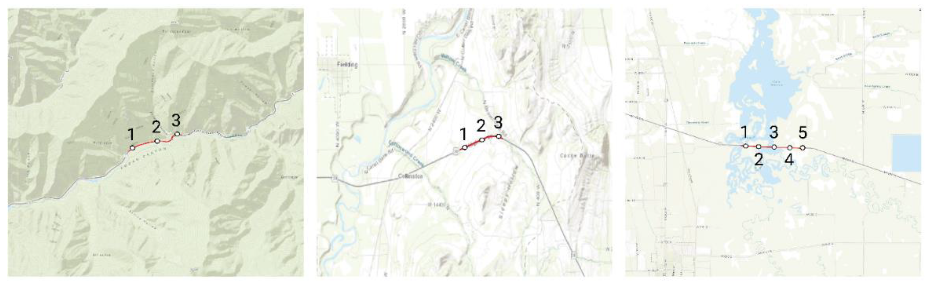
The general area selected for this study is within the authors’ home region, which made it easy to identify areas with high distinction without relying solely on publicly available geospatial data. The selection of three test sites was guided by our intimate knowledge of the area, which consists of two large mountain ranges, a well-defined topographic valley, and clearly delineated highways that intersect the valley and extend into clear passes through the mountains. To minimize the potential erroneous impacts from representing urban development, sites were selected from places identified as clearly fitting one of the three topographic conditions (mountainous, hilly, and flat) with minimal infrastructure development along a major highway. The first site selected, Logan Canyon, is within the Cache National Forest just east of Logan, UT, and is a very mountainous area. The second selected site is located on Utah Highway SR30, just northeast of Collinston, UT. This area contains some rural development and a significant amount of agricultural development with flat to undulating terrain. The surrounding terrain is filled with undulating hills and a river section that cuts through the hills to the north of our selected route. This area is mostly farmland but with the presence of the river, the area also attracts recreationists. This additional area provided us with a topographical middle ground between the mountainous and flat sites. The third site is along the Utah Highway SR30 just outside of Benson, UT where there is a large wetland on either side of the roadway, which provided sufficient terrain for our flat environment site. All the selected routes are located near popular local and regional recreational areas. A one-mile-long route was selected from each site to compare and contrast the differences in the effects of topographical properties on visual magnitude. Each site with its mile segment can be found in
Figure 2 with corresponding images of each point in
Figure 3.
2.3. Generating Viewpoints
GRAVIA was run across various viewpoint-sampling distances, and with two sampling techniques: equal interval and randomized (explained in detail later). Following [
20], we use a 10 m resolution digital terrain model (hereafter referred to as DEM) with a 1 m viewpoint-sampling distance along each route section. Note that a digital surface model was not used in this study, meaning that trees were not explicitly included, but may were captured in the DEM as part of a smoothing technique. The initial 1 m viewpoint-sampling distance was used as a base measure to create the remaining distance variations. A 1 m viewpoint-sampling interval is the equivalent to an observation every half-second for someone driving 45 MPH, which is about the speed limit of our area of study. Additional viewpoint intervals along the route included 10, 20, 30, 40, 50 and 100 m. After selecting our created one-mile route, we used the Generate Points tool in ESRI’s ArcPro to create points at a 1 m distance. We then built a model to select the sample interval for the equal interval technique and used a random-number generator to select five different viewpoint samples for the randomized sampling technique. The random generator assigned a percentage to each viewpoint so that the sampling frequency (e.g., 50% at 20 m, 25% at 40 m) selected a similar number of viewpoints relative to the equal interval stratification.
This resulted in 168 viewpoints at a 10 m distance and over 84 viewpoints at a 20 m distance in our mountain environment. In the equal interval sample, these viewpoints were spread every 20 m, while for the random sample we selected the same number of viewpoints scattered throughout the 10 m distances (resulting in some gaps of greater than 20 m). Generating viewpoints at these distances helped us gather an understanding of the degree to which we can see the surrounding environment when viewpoints are generated in a randomized fashion along a route.
2.4. Running GRAVIA
GRAVIA, referred to as the visual-magnitude plugin in [
29], was used to conduct the analyses. The plugin requires, at minimum, two input datasets: the DEM and viewpoints. The DEM was clipped to a 3 km site, which provided a reasonable radius around the one-mile route to ensure a high variety of visual-magnitude values. Each of the combinations of viewpoint-sampling-distance techniques (interval and random) was conducted separately, and the processing time for each was recorded. The output of GRAVIA is a single, 1-band, floating-point tiff file.
2.5. Running GRAVIA
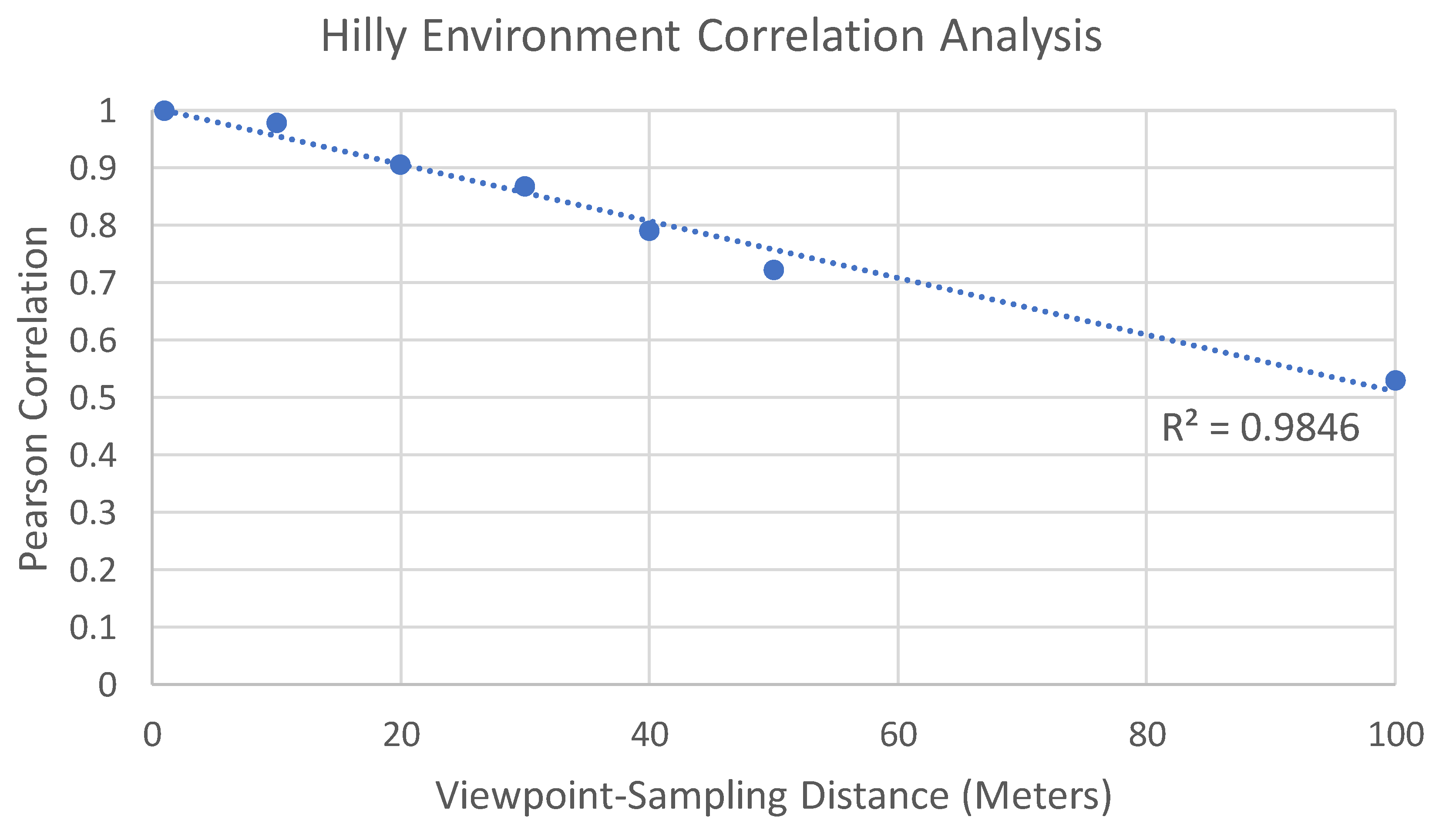
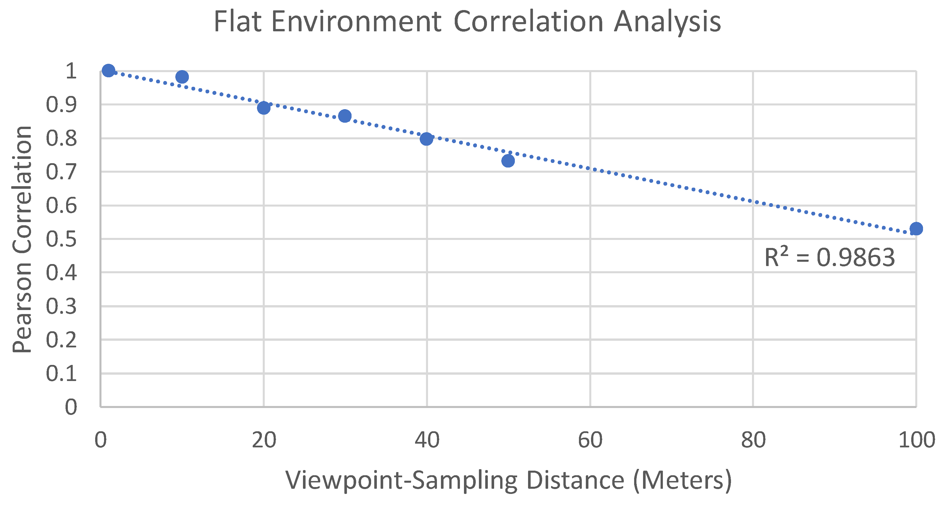
GRAVIA produces an objective normalized value from 0 to 1 for each cell of the raster output, making the comparisons somewhat straightforward. For this study, the efforts were focused on determining a Pearson correlation coefficient to identify how each of the different intervals and sampling techniques compared to one another. However, before this analysis could be produced, the data needed to be adjusted because of the differences in the total visible area (some intervals resulted in a greater visible area than others). To accomplish this, we built an analysis mask that combined all the visual-magnitude outputs into one raster where there were no null values in one or more outputs (a null value indicates that an area is not visible and cannot be analyzed by a coefficient). The mask was used to extract the visual-magnitude values for each visible cell across all analyses, ensuring that the same cell was being compared across outputs. To conduct the Pearson correlation, each raster cell value was extracted into a one-dimensional dataset and analyzed using R Statistical Software, specifically the raster package [
32]. Using ArcPro, we noted the total missing values (not part of the mask) for the analyses that were not part of the base 1 m interval. These were included as the error of the difference between the total visible area compared with the visible area from the 1 m result and all the other images. The combination of the Pearson correlation and the error provides an effective snapshot of each different sampling technique.
2.6. Multi-Ring Buffer Analyses
In addition to our preliminary analysis of our three environments, we wanted to evaluate the extent to which the distance was influenced. To accomplish this, we decided to develop a zonal distance analysis for our selected routes at distances of 100, 300, 1000, and 3000 m. Zonal distances were used to analyze data at distinct distances from the immediate vicinity (0–100 m), the middle ground (100–300 m), the visually distant area (300–1000 m), and the visual edge (1000–3000 m), though these distances were arbitrarily derived.
Figure 4. illustrates the zones for the Mountainous environment, with the one-mile segment buffered by each of the zonal distances.
This approach enabled the assessment of the variation in the results calculated by GRAVIA for areas with both immediate and distant impacts around the viewer. Note that we did not use a covariate as the distance because the distance varies based on the number of viewpoints and intervals. Instead, we used the distance buffer around the highway segment. This analysis was performed for all three environments, every viewpoint-sampling interval distance (the random was not assessed), and the four zones, totaling 84 unique outputs. A custom-coded script written for R Statistical Software was used to correlate the GRAVIA outputs for each viewpoint-sampling distance within the zone for each environment. The script read in each GRAVIA raster output file and used the Raster package raster.layerStats to calculate the correlation table.
All statistical data were consolidated or further analyzed by comparing the number of viewpoints, processing time, and the total area percentage error, with accompanying graphs generated. Additionally, all the developed maps were conducted using ESRI ArcPro. These results are provided below for each of the different study sites. Note that the correlations are reported as positive for ease of understanding, but all values are negative correlations (as interval distance increases, the correlation from GRAVIA decreases).
4. Discussion
For this paper, we sought to provide empirical evidence to address unanswered optimization questions for the site selection of route-based experiences. The primary goal of this research was to identify if there was an optimal point between the trade-off of viewpoint-sampling distance and the correlation of (visual magnitude) values produced by GRAVIA. There has been an extensive amount of work conducted on visual impact and viewshed analyses [
33], but little work comparing how the accuracy of the impact models relates to the selection of viewpoints to simulate route-based experiences. The following is a discussion of the outcomes of our findings and recommendations for future research.
The following three paragraphs explore the nuanced answer to the first research question: to identify the trade-off between the number of sample points and the accuracy of the visual-magnitude model. When we set out first to analyze the differences in sampling techniques (equal interval versus random), we had not anticipated how substantially different these techniques would be as there are a number of works that explored similar approaches [
34,
35]. Further, we expected it would be possible that one random sample could theoretically produce at least one higher correlation result than the equal interval. We did run a limited set of random viewpoint selections, so it still may be possible to find a result with a higher correlation. However, the ease of the equal interval, coupled with the exceedingly high correlation of the values at distances greater than 300 m away, suggests that the difference between an optimal and equal interval viewpoint selection may be negligible. Further, finding the optimal, or even improved random selection, is unlikely to be useful because it will take additional time. Thus, the substantial variation in the correlation with the random sample is not worth exploring. Our recommendation is to maintain an equal interval stratification of viewpoints along a route.
By conducting a multi-ring analysis, we aimed to pinpoint the relationship between distance and the accuracy of the model and answer the third research question: how does distance from the route impact the calculations across our three environments? The results indicate that the most significant changes occur within the 300 m distance, with negligible loss beyond that zone across the intervals of sampling distances explored. This is not unsurprising because GRAVIA calculates visual magnitude, which is heavily weighted by distance. Distance changes so quickly (see [
20,
28]) that differences beyond 100 m are so small that it is unlikely to result in any meaningful differences—if the space is seen. Interestingly, our percent of the total area also showed limited reductions, except around the edges of visible and not visible areas (and primarily at further distances). In the future, it would be worth exploring the relationship between the sampling distance and the distance of the area observed with sampling distances beyond 300 m. This would be useful in determining a sampling rate at which visual impact assessments need to be conducted for impacts across different distances.
To interpret our calculations, we conducted a Pearson correlation r and followed recommendations from various fields that provide insight into the meaning of the results. The results provide a correlation of the average visual-magnitude [
20] values across all the viewpoints, essentially comparing the topographical response to the viewpoint-sampling distances. So, while these data sit squarely within the physical sciences, the interpretation of these data falls within the realm of psychological sciences because we are most interested in how individuals perceive topography. To this end, we recognize that there are different interpretations between the physical and social sciences regarding Pearson’s r. In social sciences, the interpretation of Pearson’s r is somewhat well-defined, with 0.9 said to be very high (e.g., [
36]), 0.7 is strong or high positive (e.g., [
37]). However, when considering these data in terms of test–retest reliability [
38], the interpretation of correlation changes, with 0.5–0.75 as moderate reliability, 0.75–0.9 as good reliability, and 0.9 or greater as excellent reliability. However, a test–retest reliability study should be conducted with comparable sampling frequencies across different times or individual samples. In our application, values were averaged across samples, which is not a conventional test of reliability.
This paragraph provides a synthesis that answers the second research question: can we identify an optimal trade-off between the number of viewpoints needed to represent an experience and the accuracy of the visual-magnitude analysis? Based on these interpretations we make the following recommendations. First, where the analysis of an entire area is important and the environment is highly sensitive to visual impacts, aim for a 30 m interval (near 0.9 correlation), while for other landscapes, a 50 m interval seems reasonable (near 0.7 correlation). Both substantially reduce the number of viewpoints by 66% (30 m) and 80% (50 m), while balancing both the interpretation of social science correlation and reliability benchmarks. Further, it should be noted these viewpoint-sampling distances also maintain the total area seen of no less than 96%, meaning that only 4% of the area is not visible when sampled at 50 m, compared to one meter. This is likely of minimal concern because the lost areas of visibility tend to be skewed toward further distances, which individually have a much lower visual magnitude. Second, where an analysis is to be conducted for visual impacts beyond 300 m away from the route, 100 m is a reasonable sampling distance. In our three environments, we found the correlation between these different outputs to be exceedingly high. The lowest correlation value (97.3%) was found in the hilly environment, whereas the correlation was higher for the mountainous environment. We expect variation to exist for other environments, but it is unlikely to vary substantially enough.
It is important to note that these recommendations are made under some assumptions. First, we assume a large area of concern (e.g., scenic area [
39,
40]), where the visual impact may be part of or entirely this area. These results may not be as applicable to areas where impacts are being measured at near distance from observation, such as with utility corridors [
41] (unless seen from far away) and urban contexts [
42], including urban forestry and parks [
43]. Second, the screening of distant impacts should not exist in close proximity to the route. Many times, a digital terrain model (DTM) underestimates the proximal vegetation that can cause screening. In areas with high vegetation or tall trees near the route, a digital surface model could be used to compare with a DTM to ascertain potential error. Note, however, that this also assumes these trees or objects have a sense of permanence (e.g., a deciduous tree that loses foliage may not screen distant visual impacts during certain seasons). Third, the analyzed routes should not be short. Here, we demonstrated the impacts of a one-mile segment; short segments may increase the variability in the correlation values. Using a shorter segment might be relevant for large areas exposed by canyon openings along an existing route, or segments void of screening in an otherwise screened route. Deviations from these conditions may need to be explored, though one could err on the side of caution and increase the sampling interval for other cases.
Until a new optimization technique for selecting viewpoints along a route emerges, we believe that an equal interval sampling technique will provide consistent and accurate results across a range of landscapes. We do see some opportunities to refine and enrich this study. These include increasing the variety of environments, differing terrains, and urban environments in order to evaluate the influence of the built environment. We would also like to see additional measures of viewpoints explored. To address these questions, we recommend further analysis into a systematic comparison. Viewpoint-sampling distances could increase, but also decrease for pedestrian-centric experiences, and where areas nearby may carry more bearing on visual impacts. The DEM raster resolution would also be modified. A higher resolution could impact the correlation values for areas near the route. Lower resolutions might be worth exploring, particularly for areas beyond 300 m. With such high correlation values produced at this distance, it may not be relevant to run the calculations for every 10 m area. We envision a potential three-dimensional relationship between viewpoint-sampling distance, accuracy at varying distances, and differing DEM resolutions that could increase the optimization of visual impacts for very large scenic areas. There may certainly be more optimal approaches to route-based viewpoint selection, but a one-size-fits-all optimization could be challenging and may not even be worth the trade-off required to prepare the data, versus just analyzing more viewpoints.
For now, this research provides a foundation from which these additional explorations could be produced. While GRAVIA is a single example of advanced viewshed-related analyses, we suspect that these results are likely to be repeated for similar studies conducting topographically based analyses. For instance, algorithms with similar mathematics [
24,
28] are likely to experience the same errors as the distance to the observer decreases. This method could be applied to other viewshed methods that use a continuous set of viewpoints as a proxy for a continuous space of observation.
5. Conclusions
This study is one of the first to identify the trade-off between the accuracy of a viewshed analysis and the number of viewpoints along a route. Specifically, the study aimed to identify the extent to which the accuracy of a visual-magnitude model (GRAVIA) was altered based on the viewpoint-sampling distances for viewpoints along the route using a correlation analysis to compare the outcome from each distance interval. Three distinct landscapes (mountainous, hilly, and flat environments) were used for the evaluations to ensure the robustness of our findings and identify if topography had any substantial effect on the outcomes. In addition to the environments, the viewpoint-sampling tests were conducted systematically with randomized distances and equal interval distances. The equal interval distance sets were conducted on separate tests of 1, 10, 20, 30, 40, 50, and 100 m apart. All the analyses were conducted using a 10 m digital elevation model (DEM) and publicly available road data. The findings across all the interval sampling distances and environments were highly consistent and reliable. When considering the entire analysis, the loss of accuracy was minimal, with the accuracy (of correlation between 1 m and another interval) showing around half a percent drop per one-meter interval increase. Thus, when the accuracy of the entire analysis is necessary, we suggest 30 m as an ideal viewpoint-sampling distance interval for highly sensitive environments, whereas 50 m still produces a strongly correlated result for other landscapes. However, the results are more nuanced. When exploring the role of the distance from viewpoints to the landscape (not the distance between viewpoints themselves), the accuracy was substantially higher as the distance increased. We discovered that nearly all the loss in accuracy was due to the areas on the landscape closer than 300 m of proximity to the viewpoints. A 100 m sampling distance is reasonable if the area to be analyzed extends beyond 300 m. The sampling distance could be larger, given the distance on the landscape from the viewpoints, but this would need to be further examined to be certain. These recommendations establish a baseline, whereby future empirical studies can begin. We have identified the trade-off between the number of viewpoints being used along a highway route and the accuracy of the visual-magnitude-tool outputs. The work was intended to help professionals process visual impact analyses more efficiently for route-based large-area conditions.
The result of this study carries promising results for the field of visual analysis and with the exploration of other environments, data resolutions, and other variables mentioned in the discussion section, the necessary input data can be further optimized.


