Article

A GIS Plugin for Susceptibility Modeling: Case Study of Wildfires in Vila Nova de Foz Côa

1
Floradata—Biodiversidade, Ambiente e Recursos Naturais Lda, 4300-504 Porto, Portugal
2
Department of of Geosciences, Environment and Land Planning, Faculty of Sciences, University of Porto, 4169-007 Porto, Portugal
3
Earth Sciences Institute (ICT), Faculty of Sciences, University of Porto, 4169-007 Porto, Portugal
*
Author to whom correspondence should be addressed.
Land 2022, 11(7), 1093; https://doi.org/10.3390/land11071093
Submission received: 30 May 2022 / Revised: 14 July 2022 / Accepted: 14 July 2022 / Published: 17 July 2022
(This article belongs to the Special Issue Land: 10th Anniversary)

Abstract

:
Risk mapping is a crucial part of spatial planning, as it optimizes the allocation of resources in its management. It is, therefore, of great interest to build tools that enhance its production. This work focuses on the implementation of a susceptibility model for different types of spatially distributed risk in a geographic information systems (GIS) Python plugin. As an example, the susceptibility model was applied to study the occurrence of wildfires in the municipality of Vila Nova de Foz Côa, Portugal. The plugin was developed to simplify the production and evaluation of susceptibility maps regarding the available geographical information. Regarding our case study, the data used corresponds to three training areas, ten years of burned areas and nine environmental variables. The model is applied to different combinations of these factors. The validation, performed with receiver operating characteristic (ROC) curves, resulted in an area under the curve (AUC) of 74% for a fire susceptibility model, calculated with the same environmental factors used in official Portuguese cartography (land use and slope) and with the optimal training area, years of information on burned area and level of land use classification. After experimenting with four variable combinations, a maximum AUC of 77% was achieved. This study confirms the suitability of the variables chosen for the production of official fire susceptibility models but leaves out the comparison between the official methodology and the methodology proposed in this work.

1. Introduction

Wildfires constitute a phenomenon of crucial relevance in many countries. Due to a predominantly Mediterranean climate, a large number of forest fires occurs in Portugal mainland during the summer season, with a strong tendency to ravage shrubland [1,2,3,4]. With increasing rural abandonment, large-scale forestation programs and other climatic factors, the frequency and intensity of these wildfires is rising [5,6], with Portugal being one of the countries with the highest density of ignition and burned area [2,7]. The occurrence of fire events is not, as it is frequently assumed, a strictly negative phenomenon, as it can be essential for the regeneration of ecosystems classified as sensitive or even dependent on fire [8]. However, the inadequacy of spatial planning and anthropic bad practices may lead to wildfires that are prejudicial to both natural ecosystems and human civilization. In fact, most of the known causes of wildfire in northern Portugal involve intentional tort or negligence [9], and these events may lead to catastrophes, such as the one experienced by Portugal in 2017, in which Portugal was affected by two major forest fire events that occurred outside the typical forest fire season [10].
Catastrophic wildfires demand risk mapping. Here, it is important to distinguish “risk cartography” (a generalist term) from the terms “susceptibility map” (representing the propensity of an area to be affected by a given event in function of its characteristics), “hazard map” (representing the product between susceptibility and probability of occurrence, as conditioned by previous events) and “risk map” (representing specifically the product between hazard and potential damage) [11,12].
Geographical information systems (GIS) are an essential tool to generate fire risk cartography [13,14,15,16], allowing the quick and accurate analysis and combination of data from multiple sources, the manipulation of the resulting geoinformation and the generation of new data. However, the generation of complex spatial models implies the use of GIS tools that require considerable time (when using the tools one by one) and knowledge about the respective software. It would be, therefore, of great interest to have applications that facilitate the production of such maps, while still using GIS software.
In that context, some applications have been developed to facilitate the creation of fire risk cartography. For instance, Baranovskiy and Yankovich (2018) [17] created an embedded GIS software tool (under ArcGIS software) for forecasting, monitoring, and evaluating forest fire occurrence probability in Iran, using Python language. Mahmud et al. (2009) [13] developed an extensive Avenue programming script to deliver the fire vulnerability mapping in Malaysia, while allowing authorized users to edit, add or modify parameters whenever necessary, supporting fire hazard mapping using ArcView software. Bonazountas et al. (2007) [18] developed an integrated computer system based on semi-automatic satellite image processing (for fuel maps creation), socio-economic risk modelling and probabilistic models for forest fire prevention, planning and management in the island of Evoia, Greece. Gulluce and Celik (2020) [19] proposed a new fire detection method and monitoring software, FireAnalyst, for an early warning fire detection system aimed at valuable forested areas in Turkey, using the libraries of Google Maps’ application programming interface (API) in a cloud. Volokitina et al. (2021) [20] developed a fire simulation software to identify inventory plots ready to burn as well as to spread the rate for fire parts dependent upon weather conditions, predict fire intensity and fire development and calculate the required manpower and resources for fire suppression in Kazakhstan Altai.
In Portugal, a GIS open-source application [15] was already developed for the generation of risk cartography according to the specifications of the Portuguese authorities [21], which define susceptibility maps as the product between slope maps and the Corine land cover (CLC), according to the tabled values defined as a priori. Nevertheless, one can conceive of a methodology that can complement those environmental variables with others as well as using fire favorability scores that are adapted to local conditions. Based on the literature consulted, there is no other GIS application that provides intuitive tools to manipulate and generate fire risk cartography, which underlines the novelty of the proposed methodology for that purpose. Although there are other tools that are able to generate susceptibility models, to our knowledge, none of them have the flexibility to experiment with different training areas, years of occurrence and environmental variables that our tool displays.
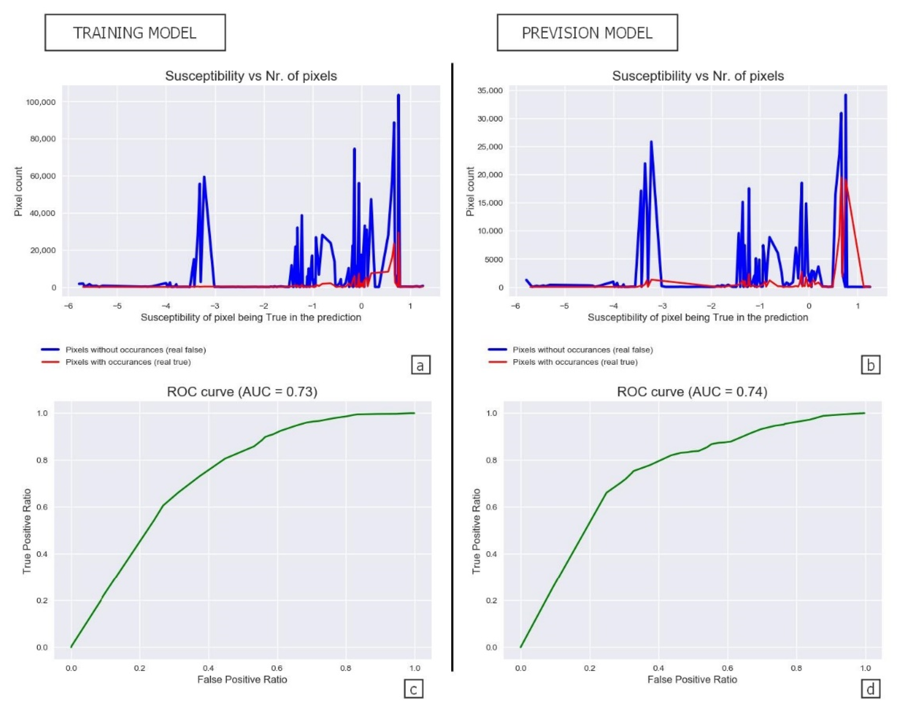
The main objective of this work is to implement a susceptibility model considering environmental variables, that can be applied to different types of natural phenomena in a GIS open-source application under QGIS software, using Python language, which is able to: (i) be applied to different types of spatially distributed risk (such as fire occurrences, landslides or other); (ii) generate a susceptibility model, for a given study area, by calculating the susceptibility scores associated with multiple environmental variables; (iii) evaluate the training and prevision models generated, calculating the area under the curve (AUC) associated to the respective regressive operational characteristic (ROC) curves [22] and (iv) optimize the model generated by selecting different training areas, years of occurrence information and environmental variables used in the model.

2. Materials and Methods

The methodology proposed in this work comprises the development of a GIS plugin in an open-source environment. Figure 1 presents the workflow of the developed GIS plugin. The processes are further discussed in this chapter, as well as the preceding data acquisition and treatment.

2.1. Study Area

The study area corresponds to the municipality of Vila Nova de Foz Côa, located on the southern bank of the Douro river (Figure 2), being an example of a territory that should have a natural relationship to wildfires, due to its strongly Mediterranean climate, yet suffered great loss in 2017.

2.2. Dataset

Geographical information relative to the study and training areas (Figure 2) were extracted from the national geographic information system (sistema nacional de informação geográfica; SNIG) search engine [23].
Data on burned areas, considering 9 years (2009–2018) of occurrences in Portugal, was obtained from institute for the conservation of nature and forests (Instituto da Conservação da Natureza e das Florestas; ICNF) geocatalog [24]. That information was converted from vectorial to raster format, attributing the value 1 to pixels burned in this period and the value 0 to the remaining pixels. Although acknowledging that not all wildfires are equal, as larger fires are more associated with extreme weather conditions and denser fuel [25,26], this work does not make a distinction between burned areas.
This work sought to include the environmental variables, which were more plausible of contributing to the prediction of a territory’s fire susceptibility, represented in Figure 3. Susceptibility models created with the official Portuguese specifications [21] uses land use and terrain slope, as do most works on fire modeling [11,27,28,29,30]. Terrain aspect is also used often [11,26,27]. Verde and Zêzere [11,26] also explore mean average precipitation (which in Portugal seems to have a positive correlation with fire when considering fuel limited fire regimes, favoring the growth of fuel) and the number of days with minimum temperatures equal or superior to 20 °C (assuming that night time suppression efforts are more likely to succeed, thanks to lower temperatures and higher air humidity). Adab (2013) [27] also suggests moisture indexes and distance to roads and urbanizations. The normalized difference vegetation index (NDVI) is mostly used for burned area detection but can also be used to access susceptibility (as it expresses fuel availability) recurrently used to study fire risk [28,31,32,33,34] and is explored in this work considering both winter and summer values. As this is a work intended to be of wider application that can be used in several and different contexts, it does not include variables, such as elevation, topographic roughness index, annual average and maximum temperature, demographic variables, fuel connectivity, fire recurrence patterns and daily climate data, mentioned in other works [2,25,29].
Land use data were obtained, in vectorial format, from Portugal’s 2018 land use map (Carta de Ocupação do Solo; COS2018) [26]. These data were converted to raster assigning different integer values to each class, for each of the 4 hierarchical levels of classification available. This has resulted in four land use images, from the most general classification to the most specific.
A map of distances to artificialized territories, representative of roads and urbanizations, was obtained from the COS2018. That map was reclassified according to Table 1.
A digital elevation model (DEM) with a 30 m of spatial resolution was obtained from Advanced Spaceborne Thermal Emission and Reflection Radiometer (ASTER) satellite data, available on the United States Geological Survey (USGS) [35]. The slope and aspect maps were generated from the DEM (using slope native algorithm from QGIS software that considers the Horn’s method by default [36]), and both were reclassified according to Table 2 and Table 3, respectively.
Satellite images with a 10 m of spatial resolution, obtained from the Multispectral Instrument (MSI) sensor onboard the Sentinel-2 were downloaded in the Copernicus European Space Agency portal [37]. Bands 8 and 4 of these images, respectively, correspondent to near infrared (NIR) and RED bands in the electromagnetic spectrum, were used to estimate NDVI for June and December 2018 (climatic extremes) according to Equation (1). That information was reclassified according to Table 4. Bands 8 and 11, respectively, correspondent to NIR and short-wave infrared (SWIR), were used to calculate the Global Vegetation Moisture Index (GVMI) for June 2018, according to Equation (2) [38]. That information was also reclassified according to Table 4.
N D V I = N I R R E D N I R + R E D
G V M I = ( N I R + 0.1 ) ( S W I R + 0.02 ) ( N I R + 0.1 ) + ( S W I R + 0.02 )
Data on total precipitation (mean annual values, in mm, for the period 1931–1960) was obtained from the national environmental information system (Sistema Nacional de Informação de Ambiente, SNIAmb) [39]. That information was converted to raster with the correspondence presented in Table 5.
Hourly data on the temperature registered by the meteorological station (with relevant data) nearest to the study area, about 29 km northwest (in Folgares), was collected from the national hydrological resources information system (Sistema Nacional de Informação de Recursos Hídricos, SNIRH) website for 2015–2021 [40].
A Python script was developed to automatically generate a .csv file with the daily minimum temperatures registered in 2018. These data were associated, in vectorial format, to the point corresponding to the station’s location. Afterward, with the DEM previously used and Montgomery K.’s rule of thumb for the variation of temperature with altitude (−1 °C for every 200 m increase) [41], 365 raster files with minimum temperatures were generated for each day of 2018 in Vila Nova de Foz Côa (Equation (3)).
T r a s t e r = T m e a s u r e d Δ T s e a + Δ T a l t
where Traster represents the value obtained in each pixel (for each of the 365 raster files), Tmeasured represents the minimum temperature measured by the station on each day, ∆Tsea represent the difference in temperature expected between the average sea level and the station (which is at a 744 m altitude) and ∆Talt represents a difference in temperature expected between the average sea level and any specific point, whose altitude was extracted from the DEM.
From these images, 365 other raster files were generated, reclassified with the value 0 in pixels where T <= 20 °C and with the value 1 in pixels where T > 20 °C. The sum of the values in those images represents the number of days with a minimum temperature equal or superior to 20 °C in each pixel of the study area. The maps of number of days with minimum temperatures equal or superior to 20 °C contained only four values (3, 4, 5, 6 and 7 days). Therefore, it was not necessary to define intervals (as it would be for a continuous scale, for example).

2.3. Implementation of the GIS Plugin

The GIS open-source application was developed under QGIS software, Version 3.16 [42]. Python programming language and several APIs and libraries were used. The “Plugin Builder” plugin was used to generate a plugin template, while the Qt Designer framework was used to stylize its graphical user interface (GUI), as seen in Figure 4. The developed GIS application is composed by a main scroll area where the user can browse for the input files—shapefiles corresponding to training and modelling areas, and raster files corresponding to a null variable (a raster image where all pixels in the extent of the study and training areas have the value “0”), at least 2 environmental variables (up to 4) and at least 2 occurrence years (up to 10)—and an area where the user can browse for the directory where the output files will be created. The “Run” button assigns those paths to string variables and passes them into the scripts described in Section 2.3.1 and Section 2.3.2, which create a susceptibility model and provide data for its evaluation.
The plugin can be downloaded at the GitHub repository linked as “Supplementary Materials” as well as a folder with some geographic information as examples. To execute the plugin on a QGIS software, the instructions in the PDF included in the folder should be followed.

2.3.1. Main Script

This work centers on the development of a Python script, named main.py, that uses the QGIS interface and processing tools to automatically generate susceptibility models. Besides importing the relevant libraries (“os” [43] and “pandas” [44]), all of the script’s content involves the definition of the “main” function, which was adapted to incorporate a plugin for QGIS (see Section 2.3). The function takes, as parameters, the instance of the plugin’s class (self), the “ROC” function (see Section 2.3.2.), the input file paths and the output folder directory.
The script starts by creating the folder where the resulting information will be saved if it does not yet exist. In this phase, it also defines the “clip” function (used recurrently in the script) and accommodates the variables that correspond to undefined occurrences and environmental variables (depending on whether or not the fields marked as optional are filled), adapting the expressions used in following calculations to those vacancies.
The script adds the geographic information corresponding to occurrences to the GIS project and calculates the sum of occurrences for each pixel (according to the expression initially defined). Afterward, it calculates a raster where the pixels with occurrences assume the value 1, and the pixels without assume the value 0 (boolean.tif) as well as a raster with the inverse logic (antiboolean.tif).
The information corresponding to the environmental variables and the occurrences (boolean and antiboolean calculated in the previous phase) is added to the project. That information is clipped by the defined training area, and the information relative to the area with occurrences is analyzed.
To calculate the susceptibility of a given area to occurrences, the informative value method was adopted. That method is usually used for analyzing the susceptibility of a territory to landslides [45,46] but also to fire [47] and other types of risk, including non-environmental [48]. The raster layer zonal statistics tool, used in the analysis mentioned in the previous paragraph, creates a table that relates the different classes of the reclassified variable (returned as “zone”) to statistics regarding the area with occurrences within such class, namely “count” (number of pixels belonging to the class) and “sum” (sum of the pixel values in the class). The function “calcular_scores”, which applies the informative value method, calculates favorability scores for each class based on the obtained statistics (Equation (4)).
l n ( b u r n e d   p i x e l s   i n   t h e   z o n e t o t a l   p i x e l s   i n   t h e   z o n e / b u r n e d   p i x e l s   i n   t h e   s t u d y   a r e a t o t a l   p i x e l s   i n   t h e   s t u d y   a r e a )
After the calcular_scores function is applied to every environmental variable, the susceptibility map is generated according to an expression that sums the score values assigned to the different pixels of the specified variables, defined initially. A reclassified map is also generated, with the values “0” changed to “0.1” for them not to interfere with the validation described in Section 2.3.2.
From that second susceptibility map, the script extracts the pixels corresponding to susceptibility in the area with occurrences (true_part.tif) and in the area without (false_part.tif), which were analyzed with the rasterlayeruniquevaluesreport tool. The resulting tables are used in the ROC function, defined in Section 2.3, to generate the first validation graphics [22].
Lastly, the script uses the calculated favorability scores to generate reclassification tables for each variable, corresponding a given score to each class. The raster files corresponding to environmental variables are then clipped by the study area and reclassified according to the scores presented in the reclassification tables. Finally, the susceptibility map corresponding to the predictive model and the associated validation graphics are generated similarly to what was described for the training model.

2.3.2. Validation Script

As discussed in Section 2.3.1., the main script generates two tables, each describing the susceptibility of each pixel to a given type of risk in the areas with occurrences (positive) or without occurrences (negative) in the study area, respectively. The information in those tables is essential for the validation of the model with the “ROC” function, imported from the validacao.py scrip.
The “ROC” function uses the “csv” [49], “matplotlib” [50] and “numpy” [51] libraries. It starts by analyzing the information contained in the tables referred to in the previous paragraph, ignoring the 0 values (in the table with the negative pixel values, the “0” corresponded to positive values; in the table with the positive pixel values, the “0” corresponded to positive values) and afterward converting the value 0.1 into 0, correcting the reclassification made in the main script. With these data, it also returns statistics correspondent to the total number of positive pixels, the total number of negative pixels and the maximum and minimum scores for the negative pixels.
The first graphic simply plots two lines, corresponding to positive and negative occurrence pixels, which represent the frequency of each susceptibility value, as seen in Figure 5. As for the second graphic, the function defines 100 thresholds—imaginary lines marking the value that separates the pixels not susceptible to the risk (on the left) from the pixels susceptible to the risk (on the right)—for the interval between the maximum and minimum negative scores. For each, it determines the false positive ratio (1-specificity) and the true positive ratio (sensibility), according to Equations (5) and (6).
f a l s e   p o s i t i v e   r a t i o = n e g a t i v e   p i x e l s   c o n s i d e r e d   a s   p o s i t i v e t o t a l   n e g a t i v e   p i x e l s
t r u e   p o s i t i v e   r a t i o = p o s i t i v e   p i x e l s   c o n s i d e r e d   a s   p o s i t i v e t o t a l   n e g a t i v e   p i x e l s
This generates 100 points of ordinates (y) defined by the true positive ratio and abscissae (x) defined by the false positive ratio, where the first point corresponds to y = 0 (no pixel is considered to be positive) and the last point corresponds to y≈1 (nearly all pixels are considered positive). The points are used to generate the ROC curve and, finally, the AUC is calculated using functions from NumPy library and the corresponding graphic is generated.
As an AUC around 0.5 represents a useless classifier (success indistinguishable from that of a random classifier), we can assume that an AUC over 0.6 is acceptable and over 0.7 is good [22]. Naturally, superior quality patterns may be used in other areas (in epidemiology, for example, a classifier with an AUC between 0.7 and 0.9 is considered to be only moderately good [52]). Nevertheless, and keeping the high complexity inherent to the theme of this study in mind, this work considers the first classification framework.

3. Results

3.1. Determination of the Ideal Training Area

To test the performance of the GIS application developed, the study area of Vila Nova de Foz Côa was used as an example. In a first phase, with the preliminary use of 6 years of burned areas and level 2 COS2018 land use classification, the developed application was applied for different training areas to evaluate which one returns the best wildfire susceptibility map for Vila Nova de Foz Côa in 2018, evaluating the AUC of the ROC curve associated to the predictive model. The municipalities west of the municipality in the same river margin (training area 1—TA1), the two municipalities in the northern margin of the river (training area 2—TA2), the four municipalities adjacent at northwest (training area 3—TA3) and the six municipalities adjacent with margins on the river (training area 4—TA4) were considered (Figure 1).
The training areas 2, 3 and 4 have produced a similar prediction AUC (Table 6). Training area 3 was chosen as it generates the best AUC for the training model.

3.2. Determination of the Most Adequate Wildfire Occurrence Period

The methodology was applied, according to the premise of using TA3 and level 2 of the COS2018, for a different number of years of information on the burned area, in order to evaluate which of them allowed the generation of a better fire susceptibility map in Vila Nova de Foz Côa in 2018. Five options were considered: 2, 4, 6, 8 and 10 years of information (Table 7).
The models generated with 2 or 4 years had a lower performance than the others—albeit they were acceptable—perhaps because there was an extensive burned area in 2017, and because some quality is derived from the simple fact that artificialized territories and water bodies are largely excluded from the burned areas. In the remaining years, the quality of the model has stabilized, indicating that the additional information becomes redundant. This may be related to the changes in the land cover, which make the information about burned areas less relevant. We chose to select the 6 years of information, respecting Ocam’s razor principle.

3.3. Determination of the Environmental Variables to Use

To determine the environmental variables that generate the most adequate susceptibility map, the developed script was applied using the combination of TA3 and 6 years of information on burned areas.

3.3.1. Determination of the Ideal COS Level

To validate the susceptibility models with the different training areas, levels 1, 2, 3 and 4 of the COS2018 were considered (Table 8).
Level 3 exhibited the best AUC for both the predictive model and the training model. Level 4 confirmed the tendency of an excessive class specification to sacrifice the quality of the predictive model for that of the training model (overfitting phenomenon), generating a prediction model equivalent to a perfectly random classification.
With that, level 3 was considered as the COS2018 analysis level that allows the generation of the best wildfire susceptibility model for Vila Nova de Foz Côa in 2018.

3.3.2. Determination of the Best Individual Environmental Variables

The developed application was executed, individually, for each variable. Land use clearly stands out as the best predictor of susceptibility to fire, while the slope is presented as the less meaningful predictor. Table 9 presents the results of the model validation for each environmental variable, while Table 10 presents the associated favorability scores.

3.3.3. Determination of the Best Combination of Environmental Variables

The susceptibility modeling plugin was executed for every pair of environmental variables with the collected data (Table 11).
Of all combinations presented in Table 11, few have returned an AUC for the predictive model greater than or equal to the one obtained with the COS2018 variable individually. One can also verify that, indeed, the land use-slope combination (Figure 5 and Figure 6) returns one of the best predictive values. In Figure 6, the area of each category would be approximately 20% of the total area (39,804 ha), which represents 7960.8 ha each.
Furthermore, it was decided to cross the combinations, which have resulted in predictive models classified as good in groups of three—combining the level 3 COS variable with all others. Table 12 shows how several of the prevision models generated using three variables exhibit a higher AUC than the one generated with the land use and slope variables, although it is a fairly small difference. Nevertheless, it was decided to cross the best trios (with AUC = 76%) with the variables involved in those crossings in combinations of four.
Table 13 presents the combinations of four variables mentioned before, where the highest AUC achieved for prediction models was 77%. This value resulted from several different combinations of variables.

4. Discussion

This work has resulted in a plugin that is able to generate susceptibility models that can be evaluated and optimized by the variation of the inputs, thus achieving the proposed objectives.
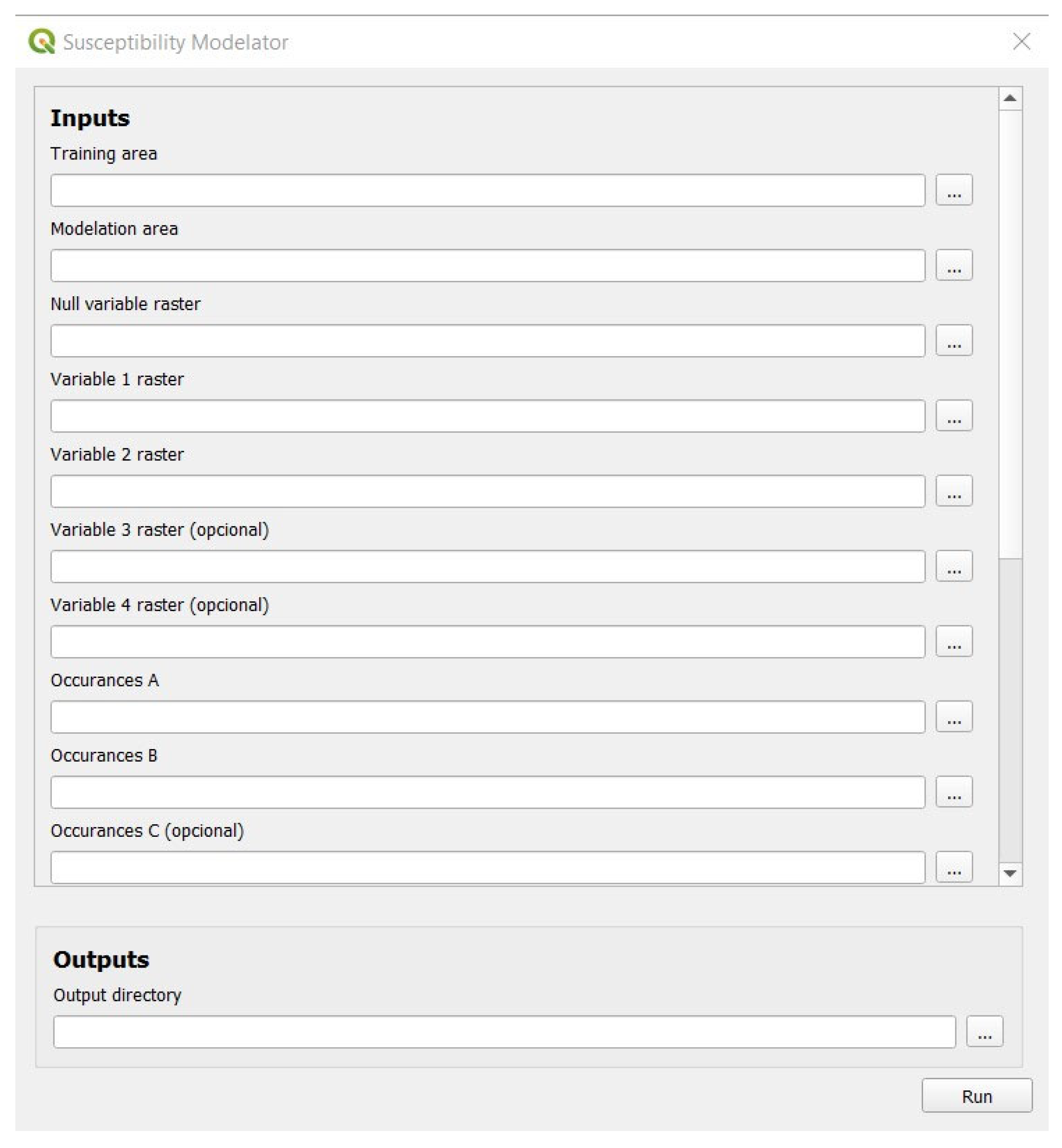
Different susceptibility models were generated by variating the shapefile used as the “Training area” input in the GUI (Figure 4). In theory, that shapefile could be a polygon with any limits insofar as it is fully covered by the raster data used as the respective occurrence inputs and environmental variable input. The same goes for the shapefile used as the “Modelation area”: this plugin can model the susceptibility of any area, as long as it is covered by both the occurrence and environmental data used.
Different susceptibility models were generated by variating the raster data just mentioned. The AUC obtained for the particular models evaluated in the results does not matter as much as the fact that it is possible to obtain such AUC and to save it, as well as the respective ROC curve graphic, for later comparison. No automatic decision algorithm was adopted for choosing the best models, mainly because the computational power required by QGIS software is substantial and programming the calculation of several models would make it excessively slow and prone to crashing, thus limiting its utility as a plugin.
The consideration of occurrence data had the logical presupposition of a single year of information being insufficient for building a good model, as well as that of decreasing utility of data with increasing age. Thus, the first model produced in that consideration involved the two earliest sets of information on risk occurrence, and the variation in the modeling was simply made by adding earlier data to the most recent data.
The consideration of environmental variables, on the contrary, involved the comparison of single variable models (achieved using a null raster as the “Variable 2 raster” input), and the variation in the number of variables used in the combination of the different variables in the double-entry Table 11, Table 12 and Table 13. In order to avoid excessive combinations in a work that is supposed to design and test the performance of a tool, the variables used in combinations of three and four were limited by imposing the presence of the best individual variable in the combinations (Level 3 COS) and later by imposing the presence of the best previous combinations.
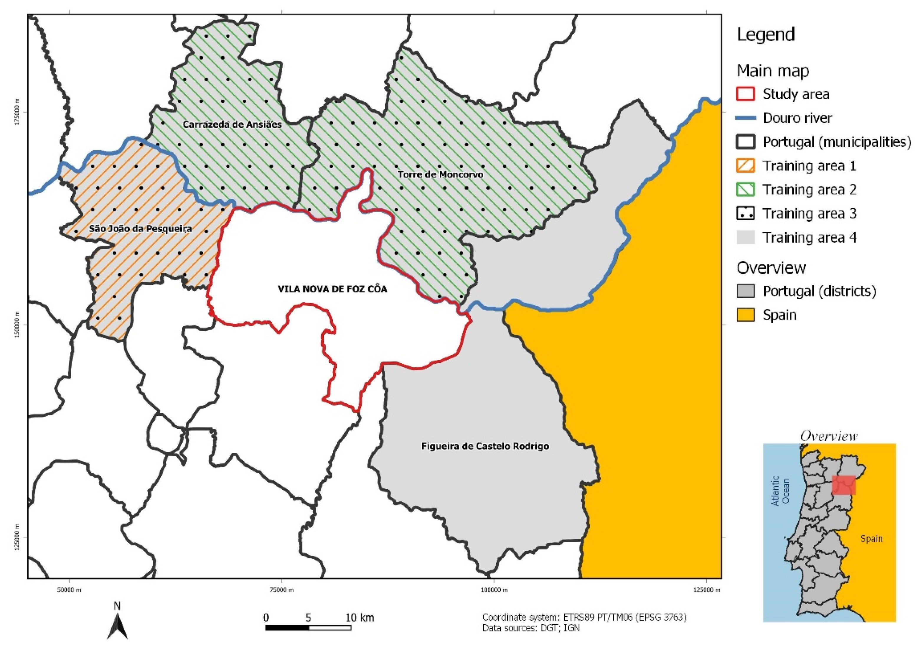
As for the results of this particular case study of wildfires in Vila Nova de Foz Côa, several points may be highlighted.
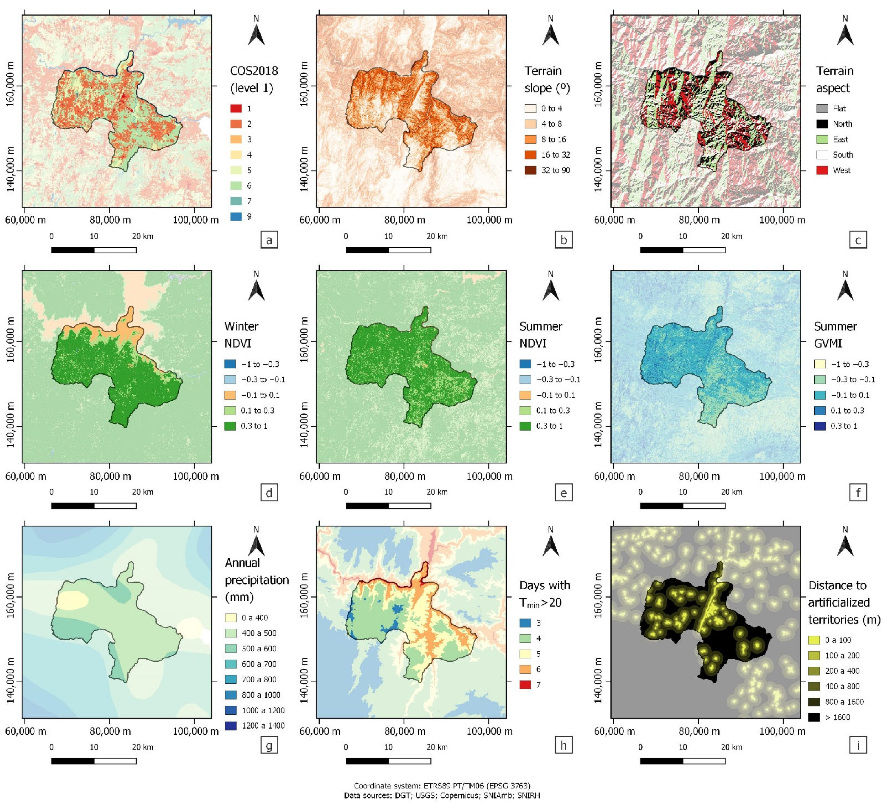
In the analysis of the susceptibility of different land use classes to fire, the sparse vegetation registered the highest score, while spontaneous grazing, agroforestry, softwood forests and shrubland were also associated with positive susceptibility values. The classes associated with artificialized territories and agriculture were invariably associated with negative scores. Previous research corroborates the results in relation to the preference of wildfires for shrubland and for softwood over hardwood [53]. The water courses class (of COS) was surprisingly associated to high susceptibility, although it is safe to say it would be related to wildfires on the riverbank of the affluents of Douro, which are usually steep (inviting easier fire spread) and occupied by shrubland.
Susceptibility generally grows with the distance. The peak of susceptibility for slope seems to occur in the middle class (8° to 16°), although the difference between the highest and lowest scores is notably small. There were also no variations in susceptibility with respect to terrain aspect, except for the extremely low score associated with flat territory (probably related to large water surfaces and human occupation), corroborated by previous studies [54]. In the winter season, the NDVI values revealed a peak in the susceptibility score for high values (> 0.3)—although there were no considerable variations—which is likely due to areas with a lower NDVI being associated with artificialized territories or water bodies. In the summer season, the NDVI revealed a considerable peak in susceptibility score for low values (< −0.3), but otherwise do not seem to exhibit a pattern. The moisture index in summertime points out to greater susceptibility with lower values, as expected, since dry fuel is more prone to burning. Precipitation shows a peak susceptibility value in the highest class and a noticeable minimum in the lowest class, which may be related (as with NDVI) to the highest growth of vegetable fuel during winter, where most Mediterranean precipitation occurs. As for the number of annual days with a minimum temperature above 20 °C, susceptibility shows a clear tendency to decrease with an increasing number of such days, contrary to what would be expected (perhaps due to the method used for temperature estimation, strictly related to altitude).
All training areas considered, composed by different combinations of surrounding municipalities, proved to adequately constitute study areas, although the four adjacent municipalities in the northwest were determined to be the best by a small margin. The ideal wildfire occurrence period seems to involve 6 years of information, which may be the point where there is enough information to allow the generation of a good model and a further amount of information will not improve it significantly. Where environmental variables are concerned, land use seems to be best used with level 3 specification when using the Portuguese COS classification, as it was found to be the best predictor of wildfires by far. When combining two environmental variables to generate a susceptibility map, every model that involved land use returned a prevision AUC > 70%, while no model that did not involve it has done so. When combining three environmental variables, several models returned a prevision AUC > 75%. When combining four environmental variables, six combinations returned a peak prevision AUC of 77%. These results can be verified in the light of the scale discussed in Section 2.3.2, which would rate an AUC over 70% as good.
The use of AUC–ROC curves has been used to validate the performance of several models [55,56,57]; however, to our knowledge, the methodology presented in this work was not applied in other studies to generate a fire susceptibility model, including the development of a GIS plugin, that enforces the use of the methodology implemented. There are several susceptibility fire models using different techniques and methods, but not compared to this methodology. For instance, Hong et al. (2018) [55] used genetic algorithms (GA) to obtain the optimal combination of forest fire-related variables and apply data mining methods for constructing a forest fire susceptibility map in Dayu County (China), validating the model performance with AUC–ROC curves. Eskandari et al. (2021) [58] also predicted the variables to be used in a model using the random forest (RF) algorithm, in Golestan Province (Iran). The use of machine learning (ML) techniques has improved the efficiency of fire prediction [59,60,61]. Kalantar et al. (2020) [56] applied adaptive regression splines (MARS), support vector machine (SVM) and boosted regression tree (BRT) to estimate fire susceptibility in Chaloos Rood (Iran), and the results were also validated using AUC–ROC curves. Zhang et al. (2019) [62] used a deep learning algorithm, particularly the convolutional neural network (CNN), to estimate a spatial prediction model for forest fire susceptibility.
The main strength of this approach for modeling susceptibility is the flexibility it offers in adapting the models to different regions, applying the methodology to different risk types, and testing different variables in search of the best model. The main weakness would be the more simplistic approach presented for evaluating the resulting models, as it can leave out several possible scenarios and is still very time-consuming, although it was conceived to achieve quicker computational processes. There is also the threat of a lack of data, particularly in terms of the past occurrence of certain types of risk, limiting the application of this model. Furthermore, the high adaptability of this plugin means the opportunity for replacing older methodologies that use fixed environmental variables, where scores are defined at the national level, in the production of regional and local risk cartography. The results obtained in this study are mostly demonstrative of the methodology implemented in the GIS application. The selection of training areas would be different and based on their similarity both in the fire regime and in the biophysical characteristics. The presentation of a single performance indicator is not sufficiently informative, especially considering the spatial homogeneity of some of the variables used in this study. Many of the ecological processes or types of hazards are context dependent, so the training models to apply them in another context will not always give good results and this should be considered in future studies.
One of the main advantages of this work was to design a flexible tool with the potential to be applied in future works. The methodology implemented in the GIS application can be used for any study area, including several training areas, if the available dataset allows it, considering the same study area with past land use and older occurrences as a training area. More environmental variables, other than the ones experimented with, can be used in search of an optimal susceptibility model, considering that the different types of wildfires can be related to different variables, which means there should be different models built for susceptibility to small, shrubland fires and to larger, high fuel load fires. Moreover, the developed GIS plugin has a wide scope in both function and language, which means it can be applied in different contexts, other than wildfires.
Risk mapping is a crucial part of land management and land planning. The possibility of predicting which areas are susceptible to a specific type of disaster, including landslides or forest fires, is unquestioned. This work analyzed the susceptibility of different land use classes to fire. The GIS plugin developed in this study is an essential tool for land management and planning, which can be used by land use planners, foresters, wildfire risk analysts and policymakers, among others.

5. Conclusions

This work presents a new GIS application, free and open-source, for generating susceptibility models, running as a plugin under QGIS software. The developed application is capable of automatically generating susceptibility models and returning ROC curves with their respective AUC values, thus facilitating the selection of the best model for use in risk cartography.
The GIS application was used for the generation of several wildfire susceptibility models in the municipality of Vila Nova de Foz Côa, Portugal, exploring different training areas, occurrence periods and environmental variables. From the results obtained, it was possible to confirm the adequacy of the environmental variables adopted by the ICNF for the calculation of wildfire susceptibility, as the model obtained with the land use and slope pair returned a prevision AUC of 74%. Nevertheless, this work does not compare this model with the one that would be obtained with the methodology used by the ICNF.
In the future, it would be interesting to compare models obtained with this methodology with models obtained with the methodology supported by official documentation. Furthermore, as this tool was designed for application in a great variety of risk cartography, such comparison should not be limited to wildfire susceptibility. Such research could prove the developed application to be useful in various contexts.

Supplementary Materials

The “Susceptibility modelator” QGIS plugin can be downloaded at: https://github.com/Andre-Padrao/susceptibility_modelator (accessed on 16 May 2022).

Author Contributions

Conceptualization, A.P.; methodology, A.P.; software, A.P.; investigation, A.P. and L.D.; data curation, A.P.; writing—original draft preparation, A.P.; writing—review and editing, A.P., L.D. and A.C.T.; funding acquisition, A.C.T. and L.D. All authors have read and agreed to the published version of the manuscript.

Funding

The work was supported by National Funds through the FCT project UIDB/04683/2020—ICT (Institute of Earth Sciences).

Institutional Review Board Statement

Not applicable.

Informed Consent Statement

Not applicable.

Data Availability Statement

Publicly available datasets were analyzed in this study. These data can be found in the links available at the references.

Acknowledgments

Carlos Bateira and Fantina Tedim, for providing the kickstart for this paper in the form of academic works. Mariana Oliveira, for the aid in building the graphical workflow.

Conflicts of Interest

The authors declare no conflict of interest.

References

  1. Pereira, M.G.; Aranha, J.; Amraoui, M. Land cover fire proneness in Europe. For. Syst. 2014, 23, 598–610. [Google Scholar] [CrossRef]
  2. Nunes, A.N. Regional variability and driving forces behind forest fires in Portugal an overview of the last three decades (1980–2009). Appl. Geogr. 2012, 34, 576–586. [Google Scholar] [CrossRef]
  3. Aranha, J.; Enes, T.; Calvão, A.; Viana, H. Shrub biomass estimates in former burnt areas using Sentinel 2 images processing and classification. Forests 2020, 11, 555. [Google Scholar] [CrossRef]
  4. Oliveira, S.; Pereira, J.; Carreiras, J. Fire frequency analysis in Portugal (1975–2005), using Landsat-based burnt area maps. Int. J. Wildland Fire 2011, 21, 48–60. [Google Scholar] [CrossRef]
  5. Tedim, F.; Remelgado, R.; Borges, C.; Carvalho, S.; Martins, J. Exploring the occurrence of mega-fires in Portugal. For. Ecol. Manag. 2013, 294, 86–96. [Google Scholar] [CrossRef]
  6. Fernandes, P.M.; Guiomar, N.; Rossa, C.G. Analysing eucalypt expansion in Portugal as a fire-regime modifier. Sci. Total Environ. 2019, 666, 79–88. [Google Scholar] [CrossRef]
  7. Turco, M.; Jerez, S.A.; Tarín-Carrasco, P.; Ratola, N.; Jiménez-Guerrero, P.; Trigo, R.M. Climate drivers of the 2017 devastating fires in Portugal. Sci. Rep. 2019, 9, 13886. [Google Scholar] [CrossRef]
  8. Meyers, R.L. Living with Fire—Sustaining Ecosystems & Livelihoods through Integrated Fire Management; The Nature Conservancy: Tallahssee, FL, USA, 2006; pp. 3–5. [Google Scholar]
  9. NICIF—Núcleo de Investigação Científica de Incêndios Florestais. Os Incêndios Florestais: Em Busca de um novo Paradigma—II Diálogo entre Ciência e Utilizadores; Faculdade de Letras da Universidade de Coimbra: Coimbra, Portugal, 2019; pp. 68–69. [Google Scholar]
  10. Novo, I.; Pinto, P.; Rio, J.; Gouveia, C. Fires in Portugal on 15th October 2017: A catastrophic evolution. In Advances in Forest Fire Research; Viegas, D.X., Ed.; Association for the Development of Industrial Aerodynamics / Forest Fire Research Centre, University of Coimbra: Coimbra, Portugal, 2018; pp. 57–70. [Google Scholar]
  11. Verde, J.C. Avaliação da Perigosidade de Incêndio Florestal. Ph.D. Thesis, School of Arts and Humanities, Departament of Geography, University of Lisbon, Lisbon, Portugal, 2008. [Google Scholar]
  12. Bachmann, A.; Allgöwer, B. A consistent wildland fire risk terminology is needed! In Fire Management Today; Brown, R.H., Dillon, M., Eds.; United States Department of Agriculture Forest Service: Washington, DC, USA, 2001; Volume 61, pp. 28–33. [Google Scholar]
  13. Mahmud, A.R.; Setiawan, I.; Mansor, S.; Shariff, A.R.M.; Pradhan, B.; Nuruddin, A. Utilization of geoinformation tools for the development of forest fire hazard mapping system: Example of Pekan fire, Malaysia. Cent. Eur. J. Geosci. 2009, 1, 456–462. [Google Scholar] [CrossRef]
  14. Akay, A.E.; Wing, M.G.; Zengin, M.; Kose, O. Determination of fire-access zones along road networks in fire-sensitive forests. J. For. Res. 2017, 28, 557–564. [Google Scholar] [CrossRef]
  15. Teodoro, A.C.; Duarte, L. Forest fire risk maps: A GIS open source application—A case study in Norwest of Portugal. Int. J. Geogr. Inf. Sci. 2013, 27, 699–720. [Google Scholar] [CrossRef]
  16. Razavi-Termeh, S.V.; Sadeghi-Niaraki, A.; Choi, S.M. Ubiquitous GIS-based forest fire susceptibility mapping using artificial intelligence methods. Remote Sens. 2020, 12, 1689. [Google Scholar] [CrossRef]
  17. Baranovskiy, N.V.; Yankovich, E.P. GIS-technologies and mathematical simulation to predict lightning-caused forest fire danger. Radio Electron. Comput. Sci. Control 2018, 1, 30–40. [Google Scholar] [CrossRef] [Green Version]
  18. Bonazountas, M.; Kallidromitou, D.; Kassomenos, P.; Passas, N. A decision support system for managing forest fire casualties. J. Environ. Manag. 2007, 84, 412–418. [Google Scholar] [CrossRef] [PubMed]
  19. Güllüce, Y.; Çelik, R.N. FireAnalyst: An effective system for detecting fire geolocation and fire behavior in forests using mathematical modeling. Turk. J. Agric. For. 2020, 44, 127–139. [Google Scholar] [CrossRef]
  20. Volokitina, A.; Kalachev, A.; Korets, M.; Sofronova, T. Fire behavior prediction in larch forests of the Kazakhstan Altai. Symmetry 2021, 13, 578. [Google Scholar] [CrossRef]
  21. Institute for Nature Conservation and Forests. Plano Municipal de Defesa da Floresta contra Incêndios (PMDFCI)—Guia Técnico; Autoridade Florestal Nacional: Lisbon, Portugal, 2012. [Google Scholar]
  22. Shengping, Y.; Gilbert, B. The receiver operating characteristic (ROC) curve. Southwest Respir. Crit. Care Chron. 2017, 5, 34–36. [Google Scholar]
  23. National Geographic Information System. Available online: https://snig.dgterritorio.gov.pt/ (accessed on 1 March 2021).
  24. Institute for Nature Conservation and Forests Geocatalog. Available online: https://geocatalogo.icnf.pt/ (accessed on 1 April 2021).
  25. Fernandes, P.M.; Loureiro, C.; Magalhães, M.; Ferreira, P.; Fernandes, M. Fuel age, weather and burn probability in Portugal. Int. J. Wildland Fire 2012, 21, 380–384. [Google Scholar] [CrossRef] [Green Version]
  26. Fernandes, P.M.; Monteiro-Henriques, T.; Guiomar, N.; Loureiro, C.; Barros, A.M. Bottom-up variables govern large-fire size in Portugal. Ecosystems 2016, 19, 1362–1375. [Google Scholar] [CrossRef]
  27. Verde, J.C.; Zêzere, J.L. Assessment and validation of wildfire susceptibility and hazard in Portugal. Nat. Hazards Earth Syst. Sci. 2010, 10, 485–497. [Google Scholar] [CrossRef]
  28. Adab, H.; Kanniah, K.D.; Solaimani, K. Modeling forest fire risk in the northeast of Iran using remote sensing and GIS techniques. Nat. Hazards 2013, 65, 1723–1743. [Google Scholar] [CrossRef]
  29. Parente, J.; Pereira, M.G. Structural fire risk: The case of Portugal. Sci. Total Environ. 2016, 573, 883–893. [Google Scholar] [CrossRef] [PubMed]
  30. Feizizadeh, B.; Omarzadeh, D.; Mohammadnejad, V.; Khallaghi, H.; Sharifi, A.; Karkarg, B.G. An integrated approach of artificial intelligence and geoinformation techniques applied to forest fire risk modeling in Gachsaran, Iran. J. Environ. Plan. Manag. 2022, 1–23. [Google Scholar] [CrossRef]
  31. Vaiopoulos, D.; Skianis, G.A.; Nikolakopoulos, K. The contribution of probability theory in assessing the efficiency of two frequently used vegetation indices. Int. J. Remote Sens. 2004, 25, 4219–4236. [Google Scholar] [CrossRef]
  32. Cheret, V.; Denux, J.P. Analysis of MODIS NDVI time series to calculate indicators of Mediterranean forest fire susceptibility. GIScience Remote Sens. 2011, 48, 171–194. [Google Scholar] [CrossRef]
  33. Florath, J.; Keller, S. Supervised machine learning approaches on multispectral remote sensing data for a combined detection of Ffire and burned area. Remote Sens. 2022, 14, 657. [Google Scholar] [CrossRef]
  34. Oliveira, E.R.; Disperati, L.; Alves, F.L. A New Method (MINDED-BA) for automatic detection of burned areas using remote rensing. Remote Sens. 2021, 13, 5164. [Google Scholar] [CrossRef]
  35. Earth Explorer. Available online: https://earthexplorer.usgs.gov/ (accessed on 1 April 2021).
  36. Horn, B.K.P. Hill shading and the reflectance map. Proc. IEEE 1981, 69, 14–47. [Google Scholar] [CrossRef] [Green Version]
  37. Open Accessed Hub. Available online: https://scihub.copernicus.eu/ (accessed on 1 May 2021).
  38. Index Data Base. Available online: https://www.indexdatabase.de/ (accessed on 1 June 2021).
  39. National Environmental Information System. Available online: https://sniamb.apambiente.pt/ (accessed on 1 March 2021).
  40. National Hydrological Resources Information System. Available online: https://snirh.apambiente.pt/ (accessed on 1 March 2021).
  41. Montgomery, K. Variation in temperature with altitude and latitude. J. Geogr. 2006, 105, 133–135. [Google Scholar] [CrossRef]
  42. Welcome to the QGIS Project! Available online: http://www.qgis.org/ (accessed on 10 March 2022).
  43. Miscellaneous Operating System Interfaces. Available online: https://docs.python.org/3/library/os.html (accessed on 10 March 2022).
  44. Python Data Analysis Library. Available online: https://pandas.pydata.org/ (accessed on 10 March 2022).
  45. Zêzere, J.L. Landslide susceptibility assessment considering landslide typology. A case study in the area north of Lisbon (Portugal). Nat. Hazards Earth Syst. Sci. 2002, 2, 73–82. [Google Scholar] [CrossRef]
  46. Oliveira, A.; Bateira, C.; Soares, L.; Faria, A.; Fernandes, J.; Hermenegildo, C.; Teixeira, M.; Gonçalves, J.A. Estabilidade de taludes em terraços agrícolas na Região Demarcada do Douro: Modelação de base estatística. In Proceedings of the VII Congresso Nacional de Geomorfologia, Lisboa, Portugal, 8–9 October 2015. [Google Scholar]
  47. Cumbane, R.N.; Zêzere, J.L. Susceptibilidade de incêndios urbanos nos bairros do município de Maputo. Rev. Científica Acad. Ciências Polic. 2018, 19–33. [Google Scholar]
  48. Araujo, A.S.; Queiroz Filho, A.P. Mapping socio-spatial segregation in the city of Marília/SP (Brazil). Rev. Bras. Geogr. Física 2018, 11, 431–441. [Google Scholar] [CrossRef] [Green Version]
  49. CSV File Reading and Writing. Available online: https://docs.python.org/3/library/csv.html (accessed on 10 March 2022).
  50. Matplotlib: Visualization with Python. Available online: https://matplotlib.org/ (accessed on 10 March 2022).
  51. The Fundamental Package for Scientific Computing with Python. Available online: https://numpy.org/ (accessed on 10 March 2022).
  52. La Torre, G. Sensitivity, specificity and ROC curves. In Applied Epidemiology and Biostatistics, 1st ed.; SEEd: Turin, Italy, 2010; pp. 261–278. [Google Scholar]
  53. Moreira, F.; Vaz, P.; Catry, F.; Silva, J.S. Regional variations in wildfire susceptibility of land-cover types in Portugal: Implications for landscape management to minimize fire hazard. Int. J. Wildland Fire 2009, 18, 563–574. [Google Scholar] [CrossRef]
  54. Carmo, M.; Moreira, F.; Casimiro, P.; Vaz, P. Land use and topography influences on wildfire occurrence in northern Portugal. Landsc. Urban Plan. 2011, 100, 169–176. [Google Scholar] [CrossRef] [Green Version]
  55. Hong, H.; Tsangaratos, P.; Ilia, I.; Liub, J.; Zhub, A.-X.; Xu, C. Applying genetic algorithms to set the optimal combination of forest fire related variables and model forest fire susceptibility based on data mining models. The case of Dayu County, China. Sci. Total Environ. 2018, 630, 1044–1056. [Google Scholar] [CrossRef] [PubMed]
  56. Kalantar, B.; Ueda, N.; Idrees, M.O.; Janizadeh, S.; Ahmadi, K.; Shabani, F. Forest Fire Susceptibility Prediction Based on Machine Learning Models with Resampling Algorithms on Remote Sensing Data. Remote Sens. 2020, 12, 3682. [Google Scholar] [CrossRef]
  57. De Santana, R.O.; Delgado, R.C.; Schiavetti, A. Modeling susceptibility to forest fires in the Central Corridor of the Atlantic Forest using the frequency ratio method. J. Environ. Manag. 2021, 296, 113343. [Google Scholar] [CrossRef]
  58. Eskandari, S.; Pourghasemi, H.R.; Tiefenbacher, J.P. Fire-susceptibility mapping in the natural areas of Iran using new and ensemble data-mining models. Environ. Sci. Pollut. Res. 2021, 28, 47395–47406. [Google Scholar] [CrossRef]
  59. Guo, Y.; Hu, S.; Wu, W.; Wang, Y.; Senthilnath, J. Multitemporal time series analysis using machine learning models for ground deformation in the Erhai region, China. Environ. Monit. Assess. 2020, 192, 464. [Google Scholar] [CrossRef]
  60. Marjanović, M.; Kovacevic, M.; Bajat, B.; Vozenílek, V. Landslide susceptibility assessment using SVM machine learning algorithm. Eng. Geol. 2011, 123, 225–234. [Google Scholar] [CrossRef]
  61. Goetz, J.N.; Brenning, A.; Petschko, H.; Leopold, P. Evaluating machine learning and statistical prediction techniques for landslide susceptibility modeling. Comput. Geosci. 2015, 81, 1–11. [Google Scholar] [CrossRef]
  62. Zhang, G.; Wang, M.; Liu, K. Forest Fire Susceptibility Modeling Using a Convolutional Neural Network for Yunnan Province of China. Int. J. Disaster Risk Sci. 2019, 10, 386–403. [Google Scholar] [CrossRef] [Green Version]
Figure 1. Workflow of the developed GIS tool.
Land 11 01093 g001
Figure 2. Framework of the study area. Municipal boundaries correspond to the Portugal official administrative map (carta administrativa oficial de Portugal; CAOP 2020).
Land 11 01093 g002
Figure 3. Environmental variables analyzed in the study: land use (a); slope (b); aspect (c); NDVI (d,e); GVMI (f); precipitation (g); days with minimum temperature > 20 °C (h); distance to artificialized territories (i). All geographical data were referenced in the European Terrestrial Reference System Portugal Transverse Mercator 2006 (ETRS89 PT/TM06) coordinate system, and raster information was all set to 30 m of spatial resolution, in order to match to the available altimetric information.
Land 11 01093 g003
Figure 4. GUI of the “Susceptibility modelator” plugin.
Land 11 01093 g004
Figure 5. Graphics generated by the developed script in the wildfire susceptibility modeling with the land use and slope variables: frequency of pixel susceptibility classification (a,b) and ROC curve for the classifier (c,d).
Land 11 01093 g005
Figure 6. Wildfire susceptibility map for Vila Nova de Foz Côa obtained by running the developed plugin with the land use and slope variables symbolized by quintiles (with linear color interpolation).
Land 11 01093 g006
Table 1. Classification of distance to artificialized territories.
Distance Interval (m)Reclassified Value
Between 0 and 100 1
Between 100 and 2002
Between 200 and 4003
Between 400 and 8004
Between 800 and 16005
Over 16006
Table 2. Terrain slope classification.
Slope Interval (°)Reclassified Value
Between 0 and 41
Between 4 and 82
Between 8 and 163
Between 16 and 324
Between 32 and 905
Table 3. Terrain aspect classification.
Aspect Interval (° North)Reclassified Value
Plain (999)0
Between 315 and 3601
Between 0 and 451
Between 45 and 1352
Between 135 and 2253
Between 225 and 3154
Table 4. NDVI and GVMI classification.
NDVI/GVMI IntervalReclassified Value
Between −1.0 and −0.31
Between −0.3 and −0.12
Between −0.1 and 0.13
Between 0.1 and 0.34
Between 0.3 and 1.05
Table 5. Precipitation classification.
Precipitation Interval (mm)Reclassified Value
Between 0 and 4001
Between 400 and 5002
Between 500 and 6003
Between 600 and 7004
Between 700 and 8005
Between 800 and 10006
Between 1000 and 12007
Between 1200 and 14008
Table 6. Results of the validation of susceptibility models generated with 6 years of burned areas, level 2 COS2018 land use classification and different training areas.
Training AreaAUC (Training)AUC (Prediction)
TA10.800.70
TA20.690.72
TA30.720.72
TA40.710.72
Table 7. Results of the validation of susceptibility models generated with training area 3, level 2 of COS2018 land use classification and different years of information on wildfire occurrences.
YearsAUC (Training)AUC (Prediction)
2 0.700.67
4 0.690.67
6 0.720.72
8 0.720.72
100.720.72
Table 8. Results of the validation of susceptibility models generated with training area 3, 6 years of occurrences and different COS levels.
COS LevelAUC (Training)AUC (Prediction)
10.700.70
20.720.72
30.730.73
40.730.5
Table 9. Results of the validation of susceptibility models generated with training area 3, 6 years of occurrences and different individual environmental variables.
VariableAUC (Training)AUC (Prediction)
COS level 30.730.73
Distance to artificialized territories0.560.57
Terrain slope0.390.39
Terrain aspect0.570.52
Winter NDVI0.420.44
Summer NDVI0.550.51
GVMI0.440.52
Precipitation0.600.35
Days with Tmin > 20 °C0.560.46
Table 10. Wildfire favorability scores generated by the developed script with training area 3, 6 years of occurrences and different individual environmental variables.
VariableClassScore
COS level 31.1.1 Continuous edified fabric−3.88
1.1.2 Discontinuous urban fabric−5.65
1.1.3 Empty spaces in built fabric−1.36
1.2.1 Industry−1.05
1.2.2 Trade−1.2
1.2.3 Agricultural facilities−2.56
1.3.1 Energy production infrastructure−3.85
1.3.2 Water infrastructure and waste treatment−2.12
1.4.1 Road and rail networks and associated spaces−5.39
1.5.1 Inert extraction areas−1.74
1.5.2 Waste deposition areas−0.13
1.5.3 Areas under construction−3.51
1.6.1 Sports equipment−2.88
1.6.2 Leisure facilities and campsites−2.41
1.6.3 Cultural equipment−1.88
1.6.4 Cemeteries−1.27
1.6.5 Other tourist equipment and facilities−3.78
1.7.1 Parks and gardens−2.12
2.1.1 Temporary rainfed and irrigated crops and rice fields−0.5
2.2.1 Vineyards−3.31
2.2.2 Orchards−0.89
2.2.3 Olive groves−1.31
2.3.1 Temporary crops and/or improved pasture associated with permanent crops−4.38
2.3.2 Complex cultural and partial mosaics−1.2
2.3.3 Agriculture with natural and semi-natural spaces−0.36
2.4.1 Protected agriculture and nurseries−1.44
3.1.1 Improved pastures−0.05
3.1.2 Spontaneous grazing0.04
4.1.1 Agroforestry0.8
5.1.1 Hardwood forests−0.13
5.1.2 Softwood forests0.15
6.1.1 Shrubland0.67
7.1.2 Bare rock−1.73
7.1.3 Sparse vegetation1.17
9.1.1 Water courses0.41
9.1.2 Water plains−0.95
Distance to artificialized territoriesBetween 0 and 100 m −2.26
Between 100 and 200−1.22
Between 200 and 400−0.73
Between 400 and 800−0.24
Between 800 and 16000.14
Over 16000.36
Terrain slopeBetween 0 and 4°−0.14
Between 4 and 8°−0.05
Between 8 and 16°0.09
Between 16 and 32°−0.01
Between 32 and 90°−0.04
Terrain aspectPlain−4.52
North−0.07
East0.27
South0.18
West−0.38
Winter NDVIBetween −1.0 and −0.3−0.45
Between −0.3 and −0.1−0.58
Between −0.1 and 0.1−0.72
Between 0.1 and 0.3−0.54
Between 0.3 and 1.00.16
Summer NDVIBetween −1.0 and −0.31.10
Between −0.3 and −0.1−0.69
Between −0.1 and 0.1−0.45
Between 0.1 and 0.30.47
Between 0.3 and 1.0−0.09
GVMIBetween −1.0 and −0.30.37
Between −0.3 and −0.10.60
Between −0.1 and 0.10.22
Between 0.1 and 0.30.53
Between 0.3 and 1.00.40
Precipitation Between 0 and 400 mm−5.58
Between 400 and 500 mm−0.27
Between 500 and 600 mm−0.00
Between 600 and 700 mm−0.26
Between 700 and 800 mm−0.32
Between 800 and 1000 mm0.68
Days with Tmin > 20 °C30.15
40.19
5−0.20
6−0.83
7−2.63
Table 11. Results of the validation of susceptibility models generated with different pairs of environmental variables. The value before the semicolon represents the training AUC, while the value after represents the prediction AUC.
Level 3 COSDistance to
Artificialized Territories
Terrain SlopeTerrain AspectWinter NDVISummer NDVIGVMIPrecipitationDays with
Tmin > 20 °C
Level 3 COS
Distance to
artificialized territories
75; 75
Terrain slope73; 7460; 64
Terrain aspect75; 7465; 6458; 55
Winter NDVI73; 7465; 6756; 6361; 59
Summer NDVI75; 7464; 6356; 5760; 5361; 59
GVMI75; 7467; 6761; 6464; 6264; 6463; 61
Precipitation75; 7167; 5961; 5065; 5163; 5463; 4768; 56
Days with
Tmin > 20 °C
74; 7267; 6058; 5062; 5057; 5061; 5066; 5964; 48
Table 12. Results of the modeling script combining level 3 COS with every other environmental variable in trios. The value before the semicolon represents the training AUC, while the value after represents the prediction AUC.
Distance to
Artificialized
Territories
Terrain SlopeTerrain AspectWinter NDVISummer NDVIGVMIPrecipitationDays with
Tmin > 20 °C
Level 3 COS + Distance (…)
Level 3 COS + Terrain slope75; 76
Level 3 COS + Terrain aspect76; 7675; 74
Level 3 COS + NDVI Winter75; 7673; 7675; 75
Level 3 COS + NDVI Summer77; 7675; 7676; 7575; 75
Level 3 COS + GVMI77; 7676; 7576; 7476; 7576; 74
Level 3 COS + Precipitation77; 7475; 7277; 7275; 7277; 7277; 72
Level 3 COS + Days Tmin > 2076; 7474; 7375; 7273; 7276; 7377; 7375; 71
Table 13. Results of the modeling script combining groups of four environmental variables. The value before the semicolon represents the training AUC, while the value after represents the prediction AUC.
Terrain AspectNDVI WinterNDVI SummerGVMI
Level 3 COS + Distance (…) + Terrain slope76; 7675; 7777; 7777; 76
Level 3 COS + Distance (…) + Terrain aspect
Level 3 COS + Distance (…) + NDVI Winter76; 77
Level 3 COS + Distance (…) + NDVI Summer78; 7677; 77
Level 3 COS + Distance (…) + GVMI78; 7678; 7778; 76
Level 3 COS + Terrain slope + NDVI Winter75; 75 78; 77
Level 3 COS + Terrain slope + NDVI Summer76; 7575; 76 78; 76
Publisher’s Note: MDPI stays neutral with regard to jurisdictional claims in published maps and institutional affiliations.

