Revealing the Land Use Volatility Process in Northern Southeast Asia

Abstract

Frequent land use change has generally been considered as a consequence of human activities. Here, we revealed the land use volatility process in northern Southeast Asia (including parts of Myanmar, Thailand, Laos, Vietnam, and China) from 2000 to 2018 with LandTrendr in the Google Earth Engine (GEE) platform based on the Normalized Burning Index (NBR). The result showed that land use volatility with similar degrees had very obvious aggregation characteristics in time and space in the study area, and the time for the occurrence of land use volatility in adjacent areas was often relatively close. This trend will become more obvious with the intensity of land use volatility. At the same time, land use volatility also has obvious spillover effects, and strong land use volatility will drive changes in the surrounding land. If combined with the land use/cover types, which are closely related to human activities that could have more severe land use volatility, and with the increase of the volatility intensity, the proportion of the land use type with strong land use volatility will gradually increase. Revealing the land use volatility process has a possibility to deepen the understanding of land use change and to help formulate land use policy.

1. Introduction

About three-quarters of the Earth’s land surface have been altered within the last millennium as a result of human activities and natural processes [1,2,3], which also brings a variety of ecological and environmental problems [4,5,6]. Changes in land use and land cover affect directly the Earth’s energy balance and the biogeochemical cycle, and also have an impact on hydrological processes and water cycles [7], climate change (precipitation and temperature) [8], carbon cycles [9], biodiversity [10], and forest degradation [11]. For example, at the expense of ecological functions, large expanses of lowland tropical rainforest have been converted to large-scale commercial plantations or small-scale mosaic agricultural landscapes in Indonesia [12]. Research has shown that there has been a pronounced loss of Amazon rainforest resilience, and one of the main reasons is deforestation and the resulting climate change since the early 2000s [2]. Then comes the impact on the carbon cycle system [13]. However, with the deepening of research, some results have shown that the global rainforest resilience and carbon sink potential of terrestrial vegetation can be increased substantially by optimal land management [14]. The impact of land use changes caused by human activities on the ecological environment is still gradually increasing [15,16,17], but the demand for environmental protection is also gradually strengthening [18,19]. Sustainable land use must therefore be identified that maintains the ecosystem and human welfare.

Land use change research has a long history, and the content is not limited by the time period or space [20,21,22]. It can be roughly divided into the assessment of the impact of land use change on the social sphere and environment, including on biodiversity or carbon emission [6,23,24], the analysis and research of the driving force of land use change, including socioeconomic drivers, institutional factors, social cultural drivers, and even transport and mobility [25,26,27,28,29], and the dynamic monitoring of land use change [30,31]. Of course, in addition to these basic research contents, there are also the development and improvement of research models for different land use change [29]. In the age of satellites, “big data”, and a growing trend of opening access to information, more scholars hope to directly quantify land use change, which is critical to addressing global societal challenges such as food security, climate change, and biodiversity loss [3]. Most of the quantification of land use change is carried out by means of satellite remote sensing, inventory, statistical data, etc., among which remote sensing satellites refer to land cover (the biophysical properties of a land surface, e.g., grassland), provide high spatial resolution, and are an effective means to detect large-scale, long-term land use changes [32]. Research has showed that global land use changes are four times greater than previously estimated [3], especially in Southeastern Asia. In recent decades, due to the rapid expansion of oil palm and rubber land, there has been rapid land conversion and land transformation in Southeast Asia [33]. These rapid succession processes represent the direct interaction between humans and the environment and provide us with the possibility to identify and understand the fluctuation process of land use.

Land use change has been extensively studied in Southeast Asia, especially deforestation [34]. Numerous studies have indicated that some intact forests have been converted to non-forest purposes, which mostly is attributed to anthropogenic drivers including logging for food production, cash crops, and agriculture, although there are diverse economic policy settings and demographics of respective countries [35]. Understanding land use change is effective for making land use regulations by integrating the features of local land use changes. Land use volatility is a manifestation of regional land use change. Understanding the process of land use volatility is a basic way of land-use-change-related research in most cases. By revealing the volatility process of regional land use, the frequency and speed of land use change can be quantified, the driving force of land use change can be further revealed, land use predictions can be made, and land use policies that conform to regional characteristics can be specified better. However, our understanding of the important volatility areas is still limited in the region, especially in the border areas of Southeast Asian countries, which have obvious characteristics of land use change due to different institutions and policies. The purposes of our research were thus to map land use volatility in an area encompassing parts of multiple countries in northern Southeast Asia (not in all of Southeast Asia) during 2000–2018 and to reveal the whole process of land use volatility. Specifically, we (1) identified the land use volatility in time and space based on Landsat images, (2) finished the cluster/outlier analysis of land use volatility, and (3) analyzed land use volatility based on land use/cover types.

2. Materials and Methods

2.1. Description of the Study Area

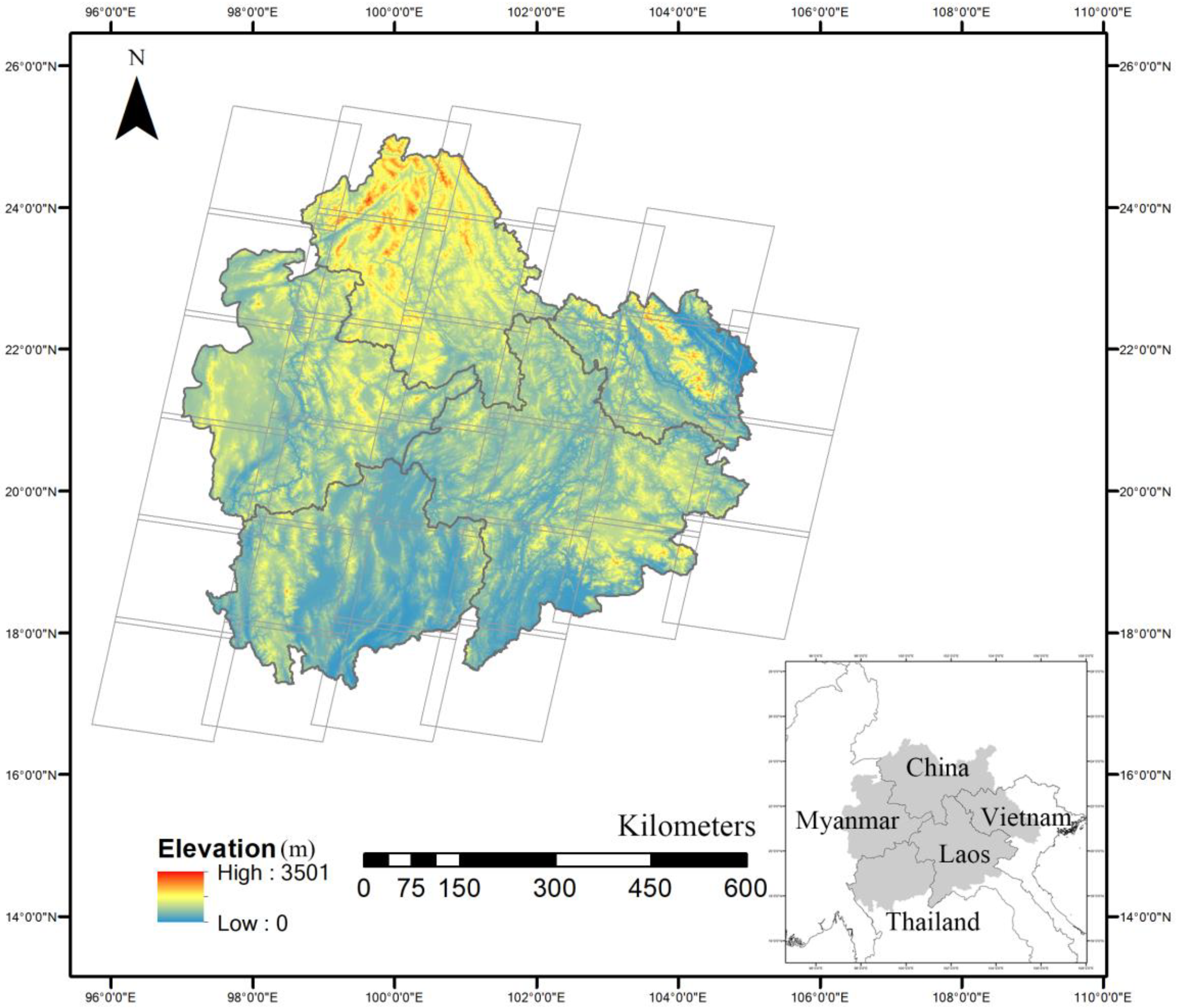
The study area is located in the northern part of the Indo-China Peninsula, geographically located between 96°45′–106°22′ E and 17°16′–25°20′ N, including eastern Myanmar, northern Thailand, northern Laos, northwest Vietnam, and China Southwestern and covering approximately 428,200 square kilometers (Figure 1). Due to its special geographical location, the regional climate is changeable with high temperature and rain. It covers a huge forest and is also a biodiversity hot spot with rapid land use transition and modification [35]. It is rich in natural rubber, rice, spices, wood, etc. According to incomplete statistics, the output of natural rubber in Southeast Asia (not limited to the research area) accounts for up to 90% of the total global output.

2.2. Priority Criteria for Data Sources

2.2.1. Satellite Images

We used Landsat 7/8 satellite images from 2000 to 2018 to assess how much land use changed in the study area. In order to ensure the accuracy and reliability of the identification of land use change, especially for the vegetation cover, the period selection of remote sensing images was mainly from May to October in each year of the study. Then, we retrieved multiple images from May to October in a year, masked out clouds and cloud shadows from each image, and created a composite of those images so that we could have reasonable annual spatial coverage of clear-view pixels.

2.2.2. Land Use/Cover Maps

Different land use types will directly affect land use volatility [37]. Considering that there is a large number of shifting cultivation behaviors in the study area, in order to reveal the relationship between land use volatility and current land use/cover types (that is, land use types in 2018), dividing land use types into land cover types closely related to shifting cultivation could be more feasible, considering the local land use characteristics. The land classification results were derived from our previous research [36].

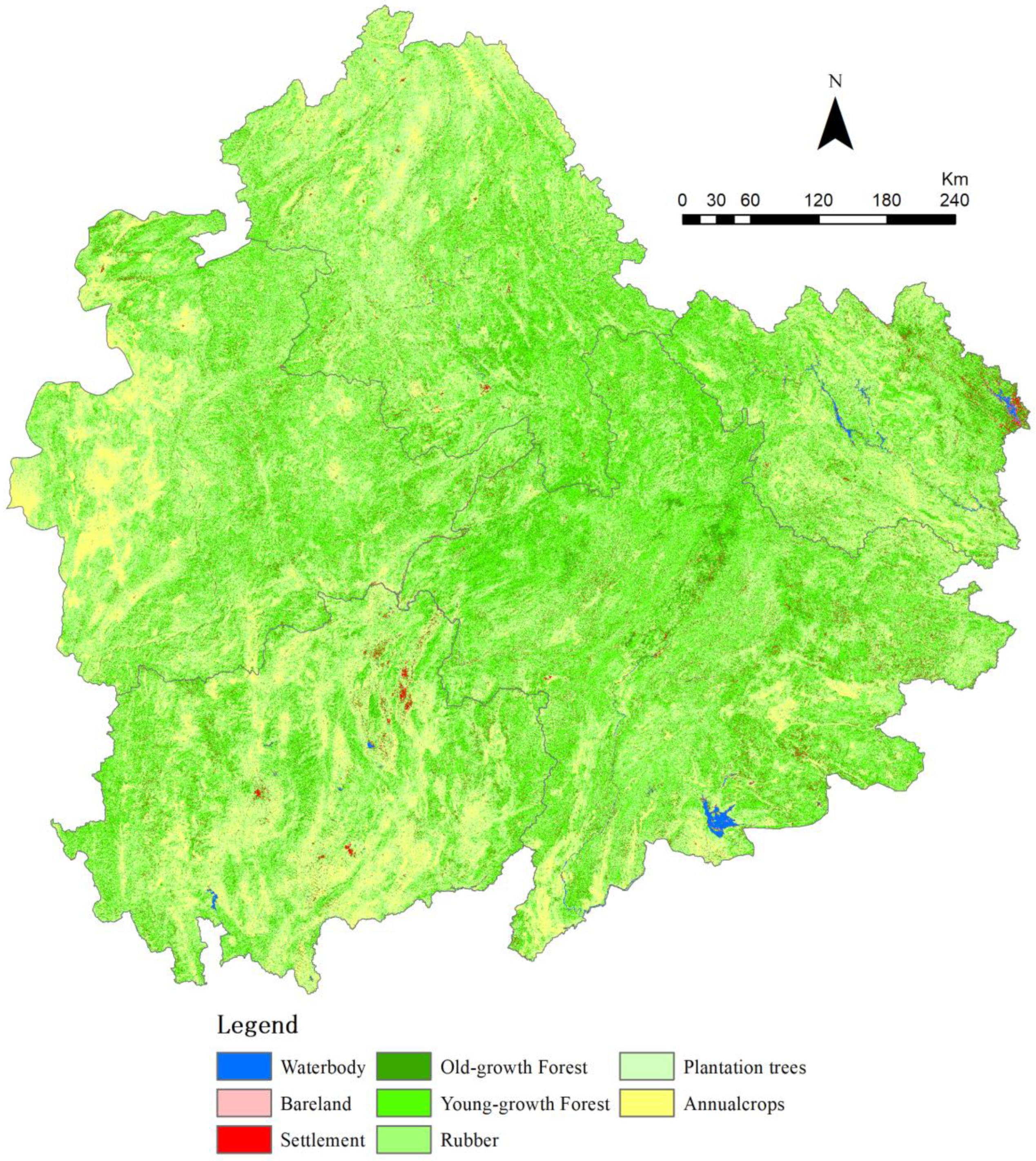
We classified the study area into the following land use types: bare land, water body, settlement, and other land use types that are often associated with land transitions and land modifications in Southeast Asia, including old growth forest, young growth forest, rubber plantations, other tree plantations, and annual crops (Figure 2) [38,39,40]. The main difference between a young-growth forest and an old-growth forest is that young-growth-forest areas have undergone shifts in cultivation in recent years; these areas were abandoned and gradually turned into forests. The post classification accuracy assessment based on a standard confusion matrix and the overall accuracy is 82.35% [36].

2.3. Methods

2.3.1. LandTrendr

Land use change will inevitably bring about changes in land cover. The LandTrendr algorithm based on Google Earth Engine (GEE) can monitor and screen such changes well [41]. Specifically, the LandTrendr algorithm is mainly based on time series analysis and extracts the relevant information of the Landsat image pixels in the study area one by one, and then calculates the spectral information correlation index of the pixel over time to select the pixels that are meaningful for the research. The principle of LandTrendr time series analysis is based on operating the algorithm to obtain the spectral information of a single pixel of the Landsat image year by year and completing the calculation of the spectral index. Then, the most important thing is further fitting it into a similar mathematical model. Based on this mathematical model, a breakpoint or an inflection point is selected, which corresponds to the pixel where the corresponding spectral index fluctuates violently, indicating that land use changes violently.

Although we use Landsat surface reflectance bands and spectral indices in our research, LandTrendr does not care what the data are, it will simply reduce the provided time series to a small number of segments and record information about when the signal changes [42].

We must guarantee that the mathematical model is fitting the spectral information of remote sensing images to improve the accuracy of the algorithm, based on understanding the operating principle of LandTrendr. There are such huge differences in different regions under the actual geographical conditions that land use/cover also have its own unique characteristics. Therefore, before the LandTrendr algorithm is actually used in a study area, it is necessary to adjust and correct the relevant parameters of the algorithm in order to ensure the accuracy and reliability of the algorithm.

2.3.2. Priority Criteria for Spectral Index Based GEE

Although the parameters’ settlement is important for the accuracy of the algorithm, the rational spectral index is also necessary for indicating land use change. There is a large amount of forest vegetation in the study area, so the spectral index mainly starts from the vegetation index. The research has shown that the NDVI index, as the normalized vegetation index, can complete the characterization of the vegetation growth state and vegetation coverage well and identify land vegetation coverage. NBR, also known as the Normalized Burning Index, is the most sensitive to forest fires and can respond well to land cover changes caused by fire sources [42,43,44]. In addition, it also has a good monitoring effect on deforestation [45].

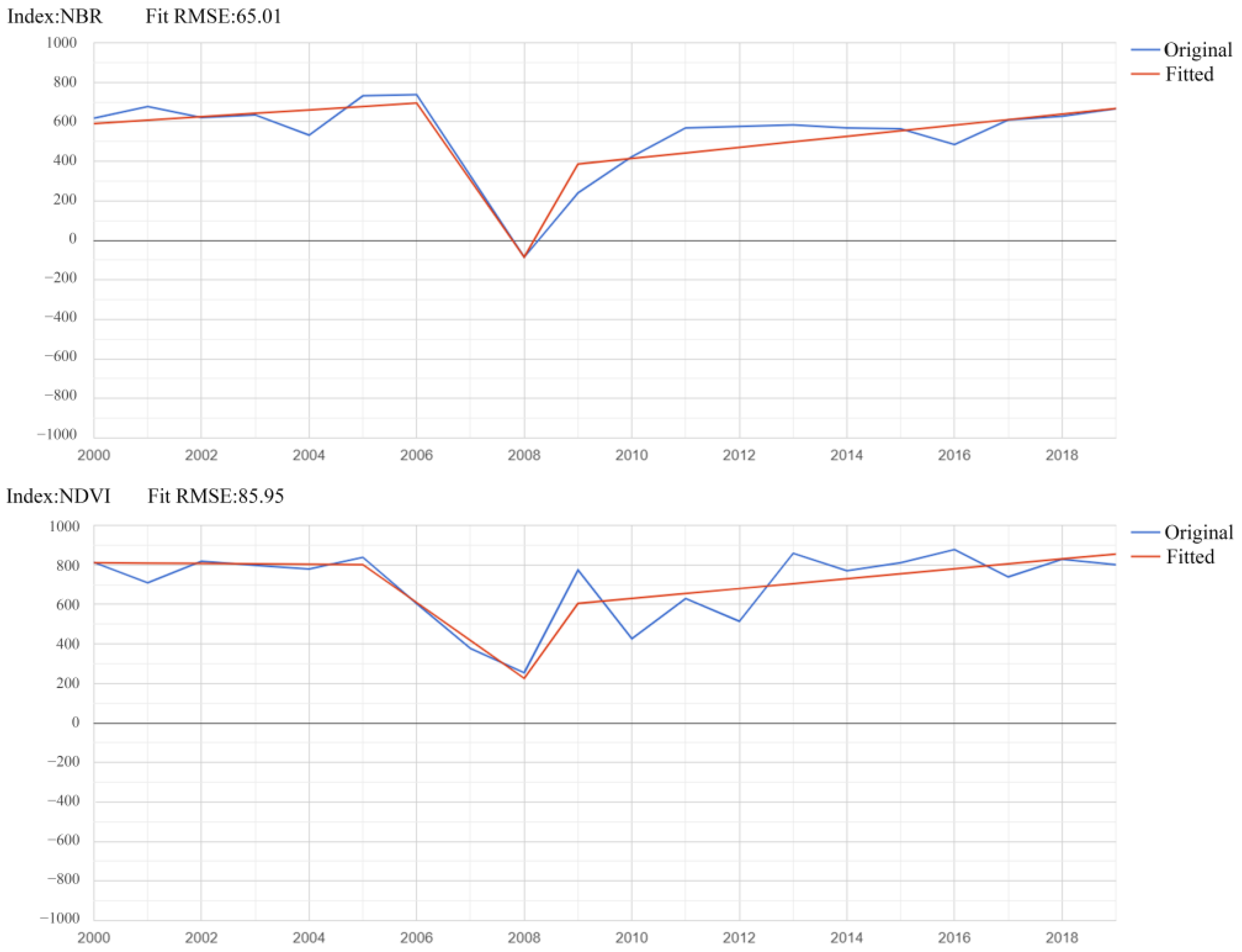
Therefore, the study mainly discussed the accuracy of vegetation change by choosing NDVI or NBR to run LandTrendr in the study area. We have checked the differences between actual spectral indices values and LandTrendr fitting mathematical models’ values per year based on NDVI and NBR after adjusting the parameters. The result showed that LandTrendr choosing the NBR as the spectral index was much better than NDVI for indicating the land use change in study area (Figure 3). All calculation results are enlarged by 1000 times to represent the details of variation.

2.4. Research Framework

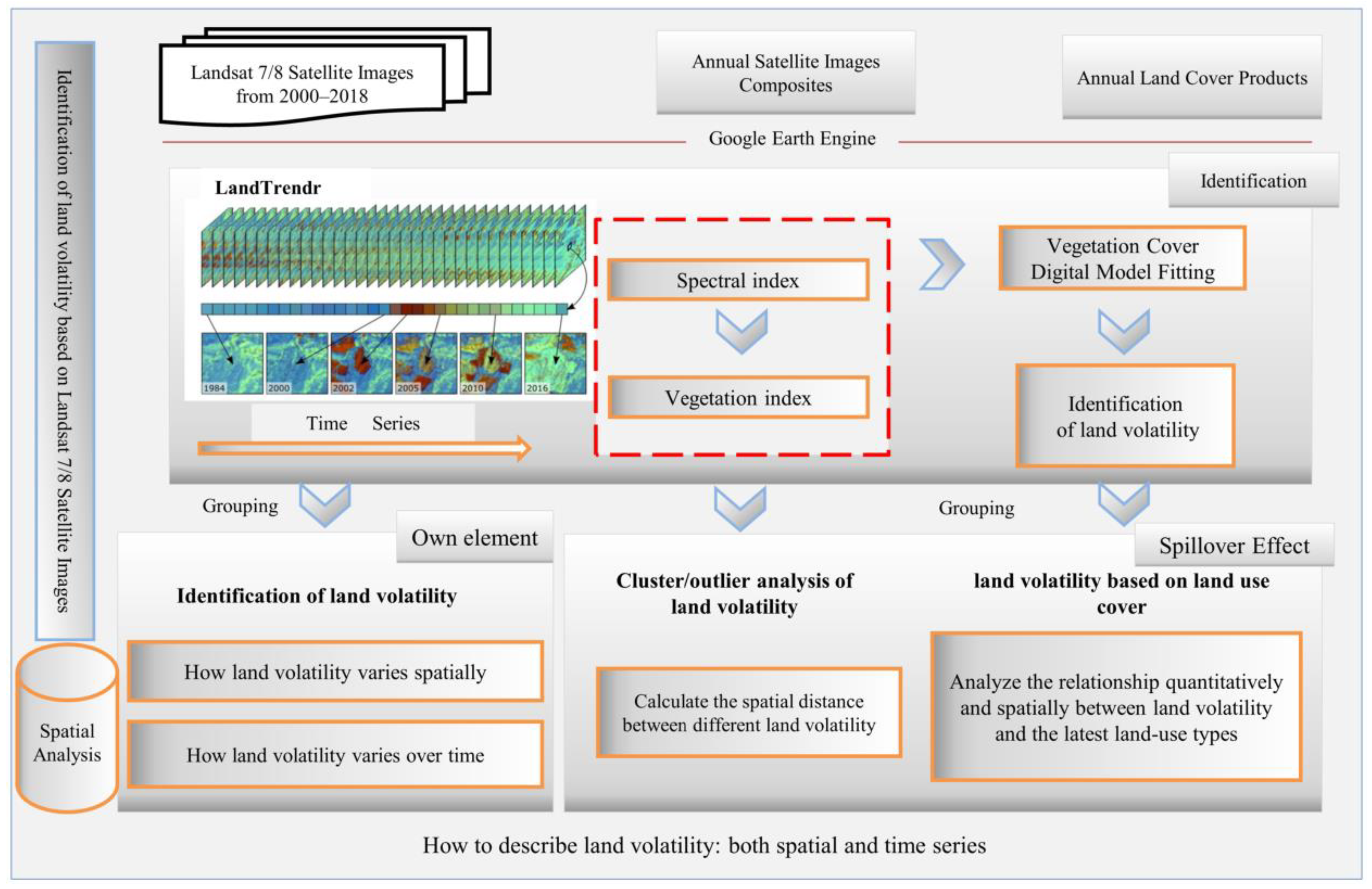
In order to assess land use change, we used LandTrendr to fit the NBR values of all pixels in the study area into the time series mathematical model and extracted abnormal inflection points or breakpoints in the trend, that is, the NBR had a large difference between adjacent years, and we used different NBR volatility values to represent different land use volatility in our research. In order to fully express the variation of the change value, we divided each 100 NBR change values into a group. Considering that when the change value was less than 100, it basically belonged to the normal fluctuation range of the calculation of satellite images, and so the change value in this interval was not considered in the study. If the change was greater than 500, which meant that the land cover type had changed greatly, we did not need to subdivide further, and all change values greater than 500 were grouped into the same group, that is, the final grouping was 100–200, 200–300, 300–400, 400–500, and more than 500, a total of 5 groups. Then, we identified the different degrees of land use volatility spatially and the basic spatial characteristics in the study area on the basis of grouping. Considering the agglomeration effect of land use [36], in order to analyze the impact of large land use volatility on the surrounding land, we measured the distance from small land use volatility (NBR < 500, that is, the change values of NBR were less than 500, the same below) to large land use volatility (NBR > 500), and finally completed the cluster/outlier analysis of land use volatility. Land use/cover types also have a significant impact on land use volatility [37], both in terms of change cycle and change time. Therefore, we further coupled the spatial relationship between the latest land use types and different land use volatility to reveal how land use affected the land use volatility (Figure 4).

3. Results

3.1. Spatial Identification of Land Use Volatility

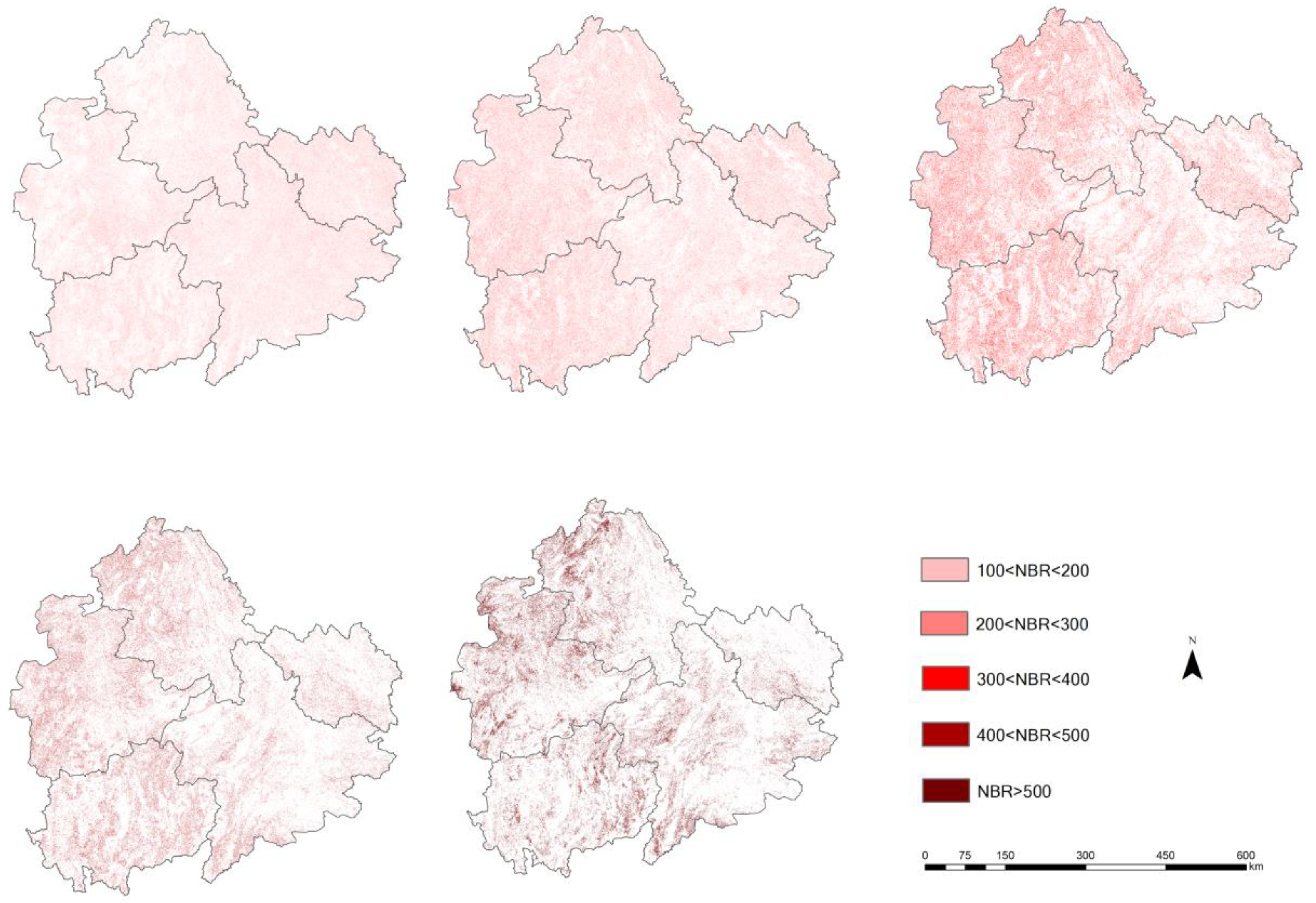
The land use volatility in the western part of the study area was larger than that in the eastern part (Figure 5). The distribution of land use patches with NBR change interval values of 100–200 was scattered, and the spatial distribution had no obvious characteristics. The distribution of land use patches with change interval values of 200–300 was relatively more balanced, and the number had also increased. The land use patches of 300–400 began to show the spatial distribution characteristics of belt-like contours along the mountains or canyons. The land use patches with NBR reduction in the range of 400–500 had an obvious aggregation effect. Until the decrement value was greater than 500, the most obvious regular change characteristics were reached. That is to say, the more the NBR value changed, the more typical were its change characteristics, indicating that the degree of interference by human activities was greater.

3.2. Temporal Identification of Land Use Volatility

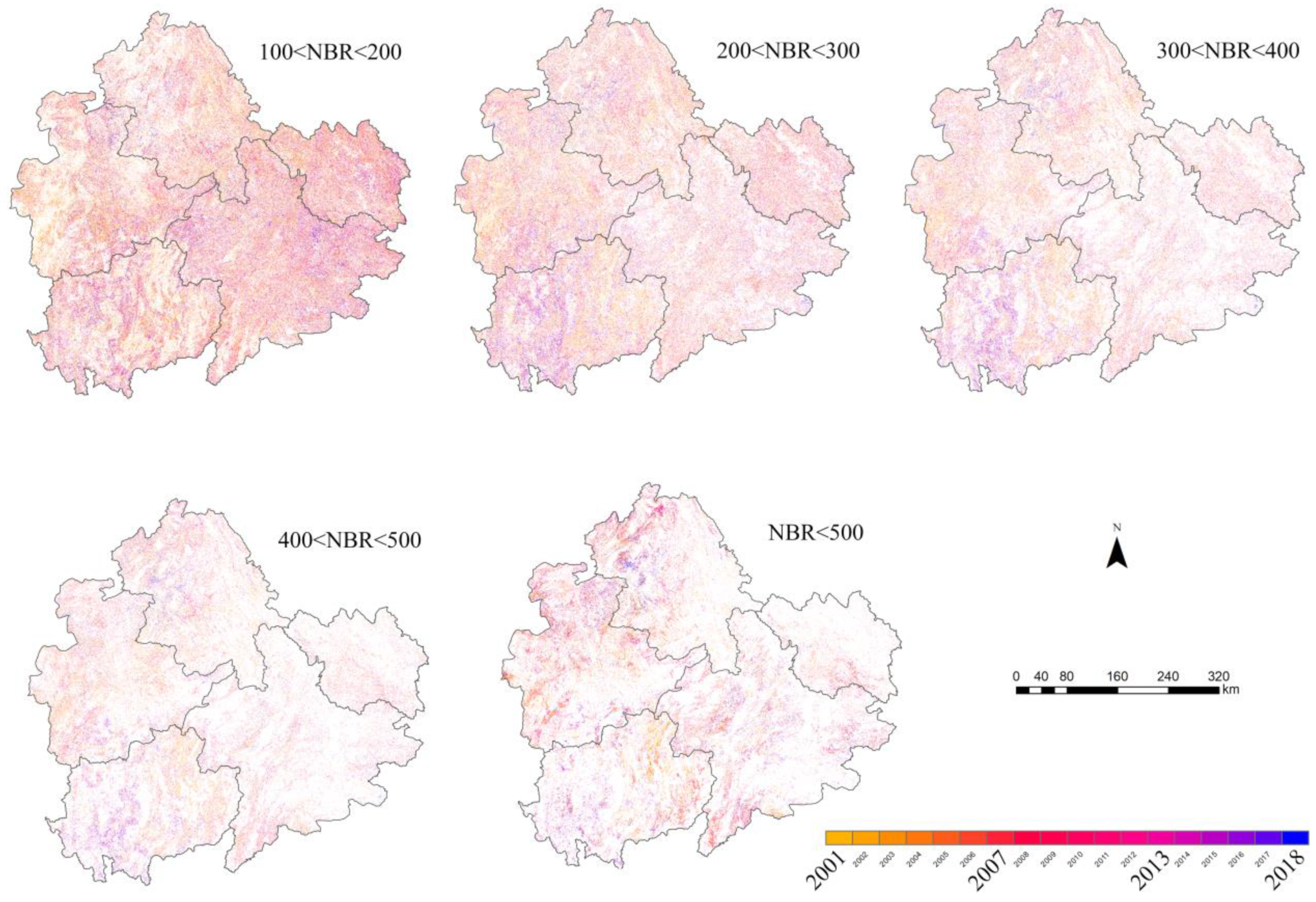
The change time of NBR reduction in the study area in the range of 100–200 was a common phenomenon, and the specific time of occurrence had no obvious characteristic (Figure 6). Land use changes of this magnitude occurred at various spatial locations in the study area in each time period, but low-intensity land use changes were not greatly affected by economic and policy coercion with relative flexibility. The change time of 200–300 began to show preliminary characteristics. The change time of the eastern region was earlier than that of the western region. The regularity of NBR reduction in the range of 300–400 also showed that the eastern region was earlier than the western region, especially in the spatially adjacent regions where the time of land use change was closer, and which preliminarily reflected the disturbance effect of human activities. A similar pattern was in the 400–500 interval of land use changes in the southwest corner occurring much later compared those in to others. The land patches with NBR value changes greater than 500, that is, areas with the most dramatic changes, were particularly concentrated in terms of time characteristics and had a very distinct band-like feature.

On the whole, the characteristics of land use change were that the northern time was earlier than that of the southern capital in the study area, and the adjacent areas with greater land use change intensity mostly occurred in the same time period. The greater the intensity, the more obvious the trend.

3.3. Cluster/Outlier Analysis of Land Use Volatility

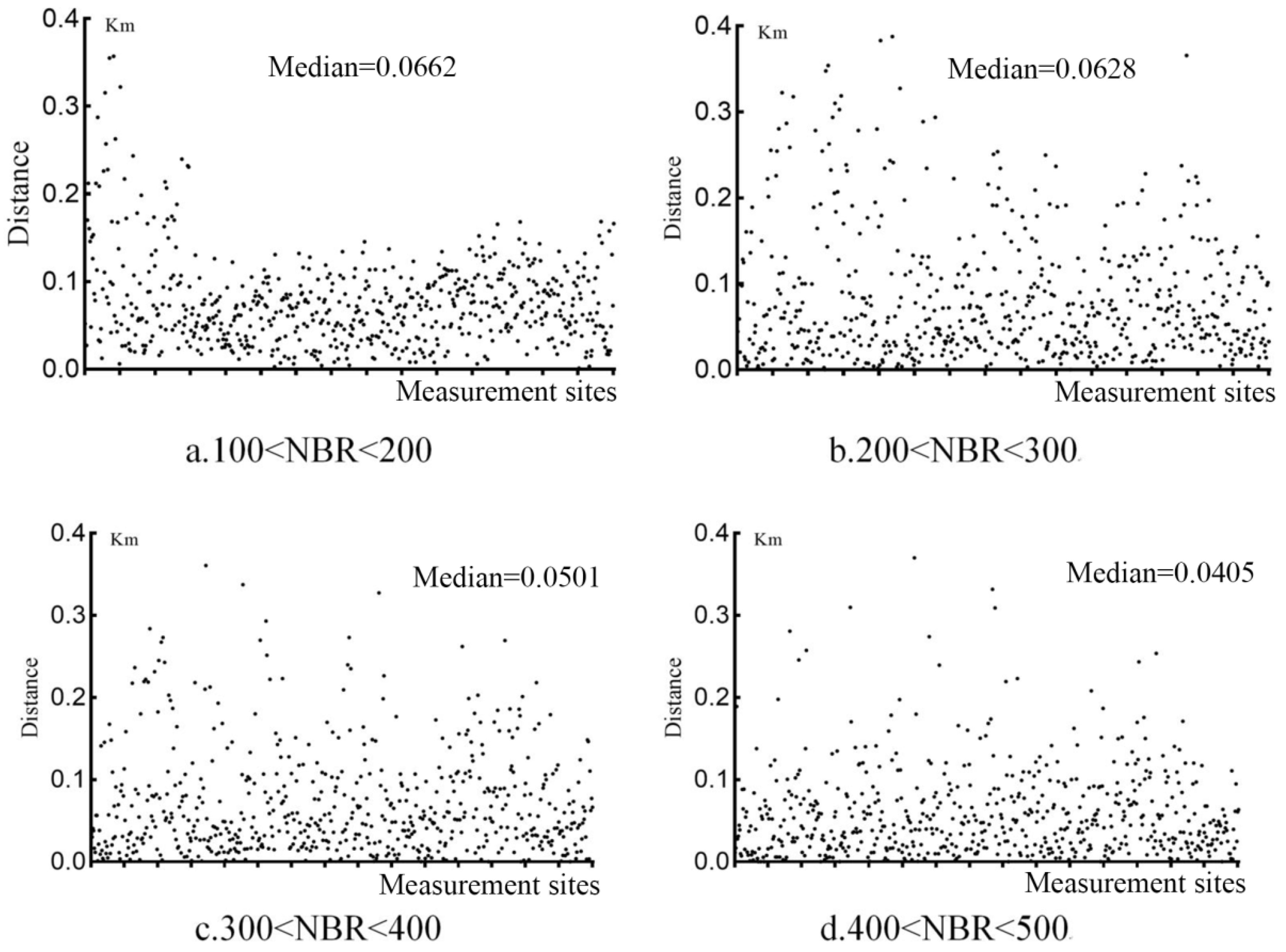
The land use volatility based on pixels in the study area showed obvious spatial trends, and there was an obvious spatial relationship between the land use change fluctuation areas identified by different NBR change values and the areas with NBR change greater than 500 (Figure 7). The land use volatility area with NBR value change of 100–200 had the most discrete distance from area with an NBR value change greater than 500, and the median distance was 67 m. The land use change fluctuation area with an NBR value change of 200–300 was also relatively close so that the median distance was 62 m. When the NBR value changed by more than 300, the distance was shortened significantly. The results showed that with NBR value changes of 300–400 and 400–500, the median distances were 50 and 41 m, respectively, which were almost bordering.

In general, most of the land use volatility areas were not more than 100 m away from each other, which also showed the agglomeration effect of human activities. The characteristic that the land use volatility weakened as the distance increased was obvious.

3.4. Land Use Volatility Based on Land Use/Cover Types

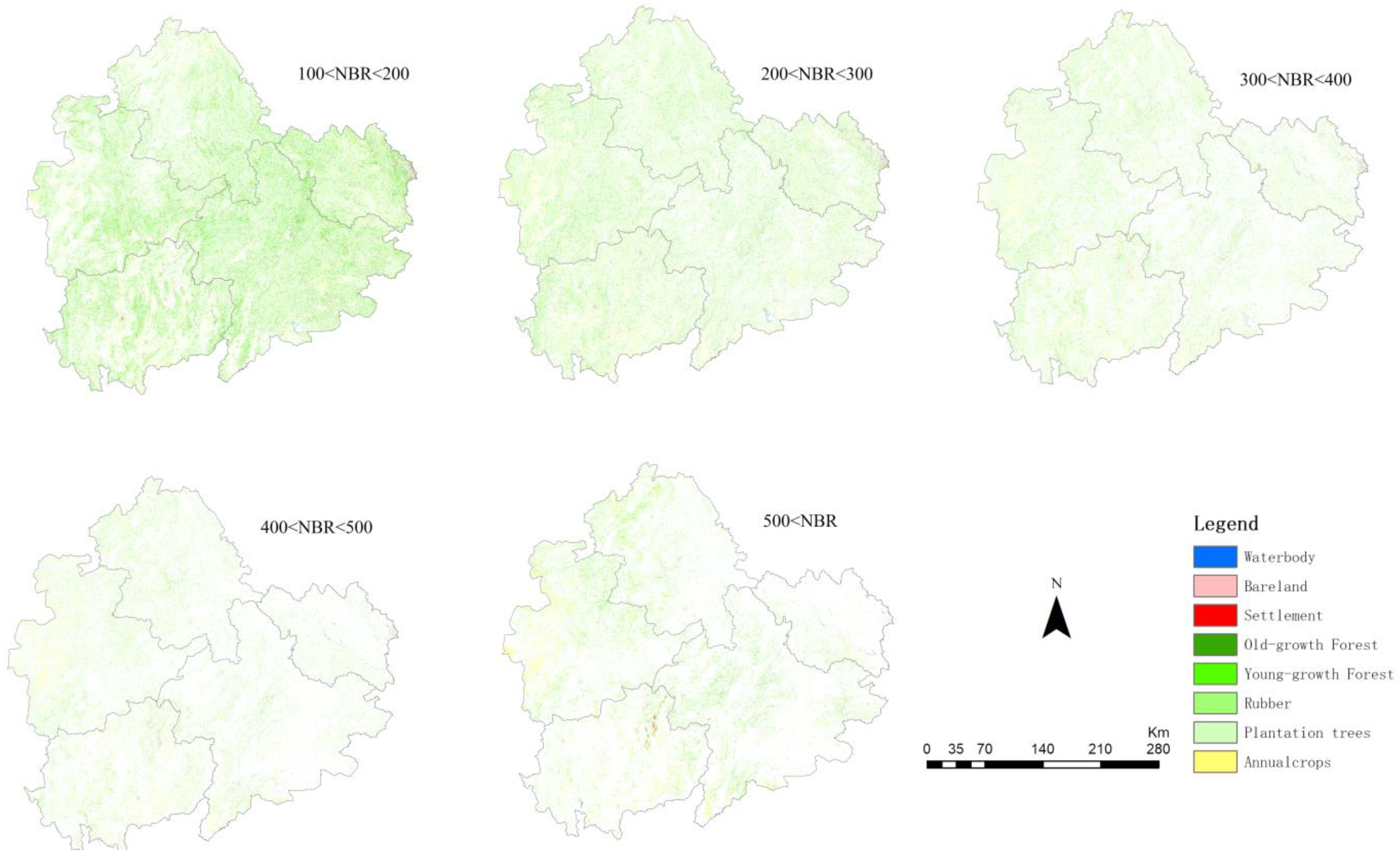
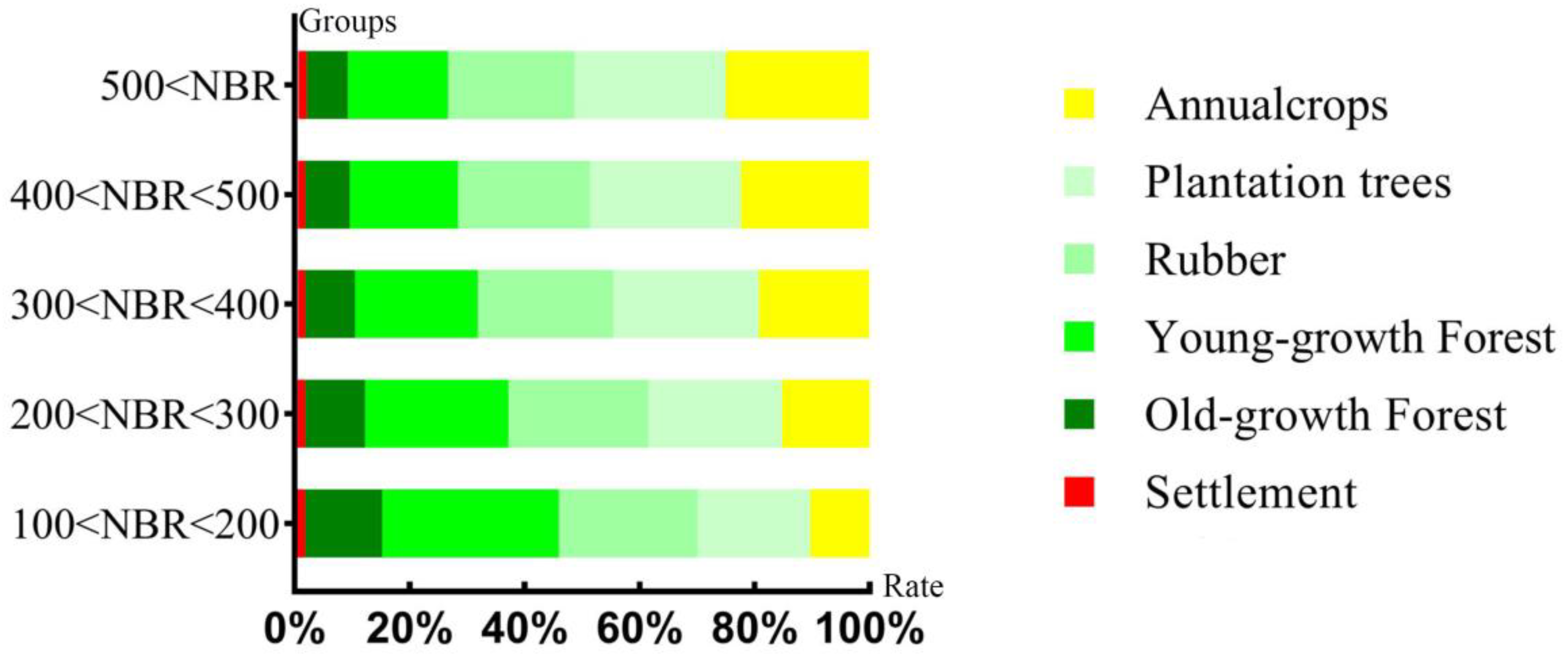
We quantitatively and spatially analyzed the relationship between land use volatility (represented by the change of NBR values) and the latest land use/cover types (that is, in 2018) during the study period (Figure 8 and Figure 9). The vast majority of land use/cover types associated with land use volatility were old- and young-growth forests, rubber, plantation trees, and annual crops, with few bare land, settlement, and waterbody types. The relationship was also different between land use volatility with various NBR values and land use/cover. The land use/cover with the largest area in the range of 100–200 was the young-growth forest, accounting for 30.65%, but the spatial distribution was relatively scattered. Young-growth forest, rubber, and plantation trees all accounted for approximately 25% in 200–300, and the spatial distribution initially appeared stripped of these land use/cover types. The situation of 300–400 was basically the same as that of 200–300, but the clustering characteristics were more obvious in the spatial distribution, such as lots of annual crops in the west of the study area. When land use volatility was in the range of 400–500 or greater than 500, the largest proportion of the area was plantation trees, accounting for 26.26% and 26.31%, respectively. Each land use type had obvious clustering characteristics in space, such as annual crops in the west area, plantation trees in the northwest area, and rubber and young-growth forest in the middle area.

With the increase of the change in NBR values, we found that in the area of the latest land use/cover type, old- and young-growth forest were gradually decreasing, and plantation trees and annual crops were gradually increasing. In contrast, the proportion of rubber didnot change significantly with the NBR fluctuation.

4. Discussions and Conclusions

4.1. Discussions

Human activities have always been one of the leading factors of land use change. Considering the direct impact of human activities on land use/cover types, regular human activities will inevitably bring about regular land use change. According to human activities, it is more reliable to explore the trend of land use change than to directly summarize the trend of land use change, and it is also one of the effective ideas of land use research. Land use volatility is more obvious due to the existence of shifting cultivation in Southeast Asia, and in the whole process of shifting cultivation, the deforestation and burning of forests will cause forest degradation, which is a direct manifestation of land use volatility, which will also lead to the loss of a large number of nutrients, loss of soil biomes, air pollution, heavy metal pollution, and ecological environments, and then indirectly affect land use change [36]. Thus, the main purpose of this article was to identify the spatial and temporal characteristics of land use volatility through different intensities of land use volatility and to analyze the impact of human activities on land use by coupling shifting cultivation related land use/cover types and then design services for regional land use planning.

The identification of land use volatility based on LandTrendr can reveal the fluctuation characteristics of regional land use changes well. Land use volatility with similar degrees had very obvious aggregation characteristics in time and space in the study area, and this trend became more obvious with the intensity of land use volatility. The small land use volatility did not have obvious characteristics in the distribution of the entire study area. We assume the main reason is that the NBR values of most land use/cover types had corresponding fluctuations in one year, which was also one of the limitations of our research method. As the volatility became larger, its spatial distribution characteristic area was obvious. The land use volatility in the west was larger than that in the east. Most of the areas with more severe land use volatility were relatively concentrated and showed the spatial distribution characteristics of the contour line along the mountain or canyon. This had a certain relationship with the limited scope of human activities, local traditional farming practices, or the level of economic development.

The time identification of land use volatility reflects the time difference and aggregation of different land use volatility. For relatively slight land use volatility, it occurs in almost all years, and the temporal trend was not particularly obvious. However, with the strengthening of land use volatility, the temporal characteristics became gradually noticeable. The time for the occurrence of land use volatility in adjacent areas was often relatively close, which showed that there was also obvious coherence in time and space. Additionally, larger land use volatility occurred in the eastern region significantly earlier than in the western region, showing a development trend in the eastern region first and in the western region later. Based on the temporal and spatial identification of land use volatility, we could conclude that land use volatility in the eastern region occurred earlier than in the western region, and the eastern region was relatively weaker than the western region during the study period.

Cluster/outlier analysis of land use volatility further illustrated the clustering effect and spillover effect of land use volatility. The distance decreased from land patches with different degrees of volatility to the NBR change value greater than 500 as the degree of land use volatility increased, that is, the greater the land use volatility, the closer the distance.

The research on land use volatility based on land use/cover once again illustrates the relationship between land use types and land use volatility. The vast majority of land use/cover associated with land use volatility were old- and young-growth forest, rubber, plantation trees, and annual crops which are related closely with human activities, and with little bare land and waterbodies. One of the main reasons for the small proportion of settlements that were also closely related to human activity was that the total amount was relatively small in the study area. Meanwhile, the relationship was also different between land use volatility with various NBR values and land use/cover. We found that in the area of the latest land use/cover, old- and young-growth forest were gradually decreasing, and plantation trees and annual crops were gradually increasing with the increase of the change in NBR values. In contrast, the proportion of rubber did not change significantly with the NBR fluctuation. These are all land use types closely related to local shifting cultivation and also illustrate the direct impact of human activities on land use volatility.

4.2. Conclusions

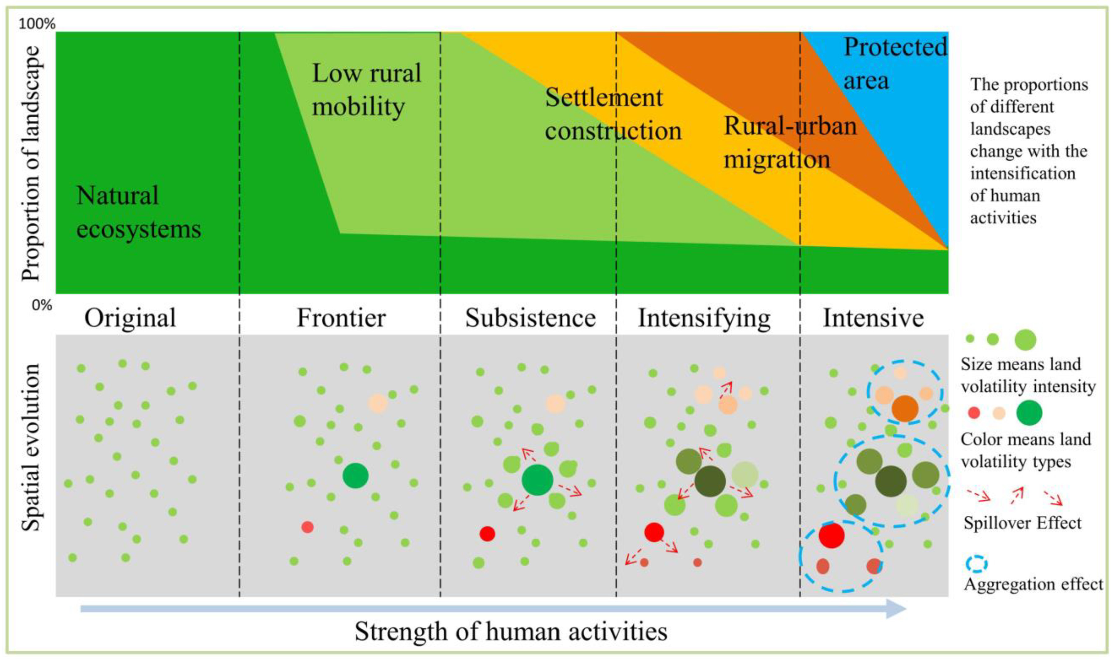
Our research shows that land use units with similar types or degrees of land use change produced a certain aggregation effect, and this aggregation effect increased with the increase of land use volatility. At the same time, these agglomeration effects manifested not only as a spatial agglomeration but also as a temporal agglomeration of land use volatility. Generally speaking, after the land use change unit had stabilized its own land use volatility, the spillover effect of its land use volatility began to appear, which will gradually drove the surrounding land use changes, thus forming a spatial aggregation. Due to this spillover effect, the generation of land use volatility showed aggregation characteristics in time, and the time was relatively close in adjacent areas of land use changes, showing a gradual diffusion trend (Figure 10). Combining different land use/cover types as a reference, the more intense human activities and the stronger the volatility of land use, the more obvious this spillover effect and trends, and the more obvious the pattern. For example, most cultivated lands were aggregated, as were settlements. The figure shows that land use volatility was relatively stable in natural ecosystems without human activities. With the occurrence of some low-intensity agricultural behaviors, land use volatility of different types and intensities began to appear. The formation of settlements further stimulates the occurrence of land use volatility. When land units cannot meet the demands of the land, the mutual migration between rural and urban regions will further stimulate the occurrence of land use volatility and this will further spread the land use volatility outward from the initial utilization unit. Finally, the land use volatility aggregation effect is formed in time and space. There will also be protected areas based on the need for ecological environmental protection, which corresponds to the gradual weakening of land use volatility in the later period.

The characteristics of land use evolution are basically similar in most regions, but the final states were quite different. The differences were due to local natural conditions, geographical environment, economic conditions, land policies, etc. It is necessary to fully consider its own key elements in order to formulate a reasonable land use policy, on the basis of combining the characteristics of land use volatility.

4.3. Limitations and Uncertainties

This study investigated regional land use volatility, and the ideas have certain reference significance for the long-term land use change research. Compared with previous studies, this paper realized the extraction of regional land use volatility based on NBR on a longer time scale and explored the whole process of land use volatility changes based on the combination of land use volatility time characteristics, spatial characteristics, and the relationship with land use types. The accuracy of the research results was directly affected by the extraction results of land use volatility to a certain extent in this paper. Since the research only used one spectral index fitting model for land use volatility, the accuracy of the final results may have been affected, but considering that the core purpose was regional land use volatility trends of this study, the results have a certain degree of reliability.

The simulation of the land use volatility process was mainly based on the time and space fitting under the theoretical conditions. There was no specific discussion on the specific land system impact, land policy intervention, urban construction stage, and other conditions. Subsequent research should consider the differences in the land use change process caused by factors such as national institutions, land policies, production methods, and crop products, and the results could be more practical. For example, functional zoning absolutely has the capacity to regulate land use volatility, and if we can better understand the impact of the setting of functional zones on land use volatility, it will have good guiding significance for arranging land rationally. Although the research results are not applicable to all countries and regions, they are of practical significance for understanding regional land use volatility and grasping the temporal and spatial differences of land use volatility. This study idea is helpful to improving land use management measures and providing suggestions.

References

- Ettehadi Osgouei, P.; Sertel, E.; Kabadayı, M.E. Integrated usage of historical geospatial data and modern satellite images reveal long-term land use/cover changes in Bursa/Turkey, 1858–2020. Sci. Rep. 2022, 12, 9077. [Google Scholar] [CrossRef] [PubMed]
- Boulton, C.A.; Lenton, T.M.; Boers, N. Pronounced loss of Amazon rainforest resilience since the early 2000s. Nat. Clim. Chang. 2022, 12, 271–278. [Google Scholar] [CrossRef]
- Winkler, K.; Fuchs, R.; Rounsevell, M.; Herold, M. Global land use changes are four times greater than previously estimated. Nat. Commun. 2021, 12, 2501. [Google Scholar] [CrossRef] [PubMed]
- Barnes, A.D.; Jochum, M.; Mumme, S.; Haneda, N.F.; Farajallah, A.; Widarto, T.H.; Brose, U. Consequences of tropical land use for multitrophic biodiversity and ecosystem functioning. Nat. Commun. 2014, 5, 5351. [Google Scholar] [CrossRef]
- Bai, Y.; Wong, C.P.; Jiang, B.; Hughes, A.C.; Wang, M.; Wang, Q. Developing China’s Ecological Redline Policy using ecosystem services assessments for land use planning. Nat. Commun. 2018, 9, 3034. [Google Scholar] [CrossRef] [Green Version]
- Cao, F.; Dan, L.; Ma, Z.; Gao, T. Assessing the regional climate impact on terrestrial ecosystem over East Asia using coupled models with land use and land cover forcing during 1980–2010. Sci. Rep. 2020, 10, 2572. [Google Scholar] [CrossRef]
- Szpakowska, B.; Świerk, D.; Dudzińska, A.; Pajchrowska, M.; Gołdyn, R. The influence of land use in the catchment area of small waterbodies on the quality of water and plant species composition. Sci. Rep. 2022, 12, 7265. [Google Scholar] [CrossRef]
- Trenberth, K.E. Rural land-use change and climate. Nature 2004, 427, 213. [Google Scholar] [CrossRef]
- Li, Y.; Brando, P.M.; Morton, D.C.; Lawrence, D.M.; Yang, H.; Randerson, J.T. Deforestation-induced climate change reduces carbon storage in remaining tropical forests. Nat. Commun. 2022, 13, 1964. [Google Scholar] [CrossRef]
- Jung, M.; Rowhani, P.; Scharlemann, J.P.W. Impacts of past abrupt land change on local biodiversity globally. Nat. Commun. 2019, 10, 5474. [Google Scholar] [CrossRef] [Green Version]
- Davis, K.F.; Koo, H.I.; Dell’Angelo, J.; D’Odorico, P.; Estes, L.; Kehoe, L.J.; Kharratzadeh, M.; Kuemmerle, T.; Machava, D.; Pais, A.d.J.R.; et al. Tropical forest loss enhanced by large-scale land acquisitions. Nat. Geosci. 2020, 13, 482–488. [Google Scholar] [CrossRef]
- Clough, Y.; Krishna, V.V.; Corre, M.D.; Darras, K.; Denmead, L.H.; Meijide, A.; Moser, S.; Musshoff, O.; Steinebach, S.; Veldkamp, E.; et al. Land-use choices follow profitability at the expense of ecological functions in Indonesian smallholder landscapes. Nat. Commun. 2016, 7, 13137. [Google Scholar] [CrossRef] [PubMed]
- Pütz, S.; Groeneveld, J.; Henle, K.; Knogge, C.; Martensen, A.C.; Metz, M.; Metzger, J.P.; Ribeiro, M.C.; de Paula, M.D.; Huth, A. Long-term carbon loss in fragmented Neotropical forests. Nat. Commun. 2014, 5, 5037. [Google Scholar] [CrossRef] [PubMed] [Green Version]
- Sha, Z.; Bai, Y.; Li, R.; Lan, H.; Zhang, X.; Li, J.; Liu, X.; Chang, S.; Xie, Y. The global carbon sink potential of terrestrial vegetation can be increased substantially by optimal land management. Commun. Earth Environ. 2022, 3, 8. [Google Scholar] [CrossRef]
- Seneviratne, S.I.; Phipps, S.J.; Pitman, A.J.; Hirsch, A.L.; Davin, E.L.; Donat, M.G.; Hirschi, M.; Lenton, A.; Wilhelm, M.; Kravitz, B. Land radiative management as contributor to regional-scale climate adaptation and mitigation. Nat. Geosci. 2018, 11, 88–96. [Google Scholar] [CrossRef]
- Gao, P.; Niu, X.; Wang, B.; Zheng, Y. Land use changes and its driving forces in hilly ecological restoration area based on gis and rs of northern china. Sci. Rep. 2015, 5, 11038. [Google Scholar] [CrossRef] [Green Version]
- Bryan, B.A.; Gao, L.; Ye, Y.; Sun, X.; Connor, J.D.; Crossman, N.D.; Stafford-Smith, M.; Wu, J.; He, C.; Yu, D.; et al. China’s response to a national land-system sustainability emergency. Nature 2018, 559, 193–204. [Google Scholar] [CrossRef]
- Popp, A.; Humpenöder, F.; Weindl, I.; Bodirsky, B.L.; Bonsch, M.; Lotze-Campen, H.; Müller, C.; Biewald, A.; Rolinski, S.; Stevanovic, M.; et al. Land-use protection for climate change mitigation. Nat. Clim. Chang. 2014, 4, 1095–1098. [Google Scholar] [CrossRef]
- Fuldauer, L.I.; Thacker, S.; Haggis, R.A.; Fuso-Nerini, F.; Nicholls, R.J.; Hall, J.W. Targeting climate adaptation to safeguard and advance the Sustainable Development Goals. Nat. Commun. 2022, 13, 3579. [Google Scholar] [CrossRef]
- Foley, J.A.; DeFries, R.; Asner, G.P.; Barford, C.; Bonan, G.; Carpenter, S.R.; Chapin, F.S.; Coe, M.T.; Daily, G.C.; Gibbs, H.K.; et al. Global Consequences of Land Use. Science 2005, 309, 570–574. [Google Scholar] [CrossRef] [Green Version]
- Jepsen, M.R.; Kuemmerle, T.; Muller, D.; Erb, K.; Verburgf, P.H.; Haberl, H.; Vesterager, J.P.; Andric, M.; Antrop, M.; Austrheim, G.; et al. Transitions in European land-management regimes between 1800 and 2010. Land Use Policy 2015, 49, 53–64. [Google Scholar] [CrossRef]
- Meyfroid, P.; Chowdhury, R.R.; de Bremond, A.; Ellis, E.C.; Erb, K.H.; Filatova, T.; Garrett, R.D.; Grove, J.M.; Heinimann, A.; Kuemmerle, T.; et al. Middle-range theories of land system change. Glob. Environ. Chang. Hum. Policy Dimens. 2018, 53, 52–67. [Google Scholar] [CrossRef]
- De Baan, L.; Alkemade, R.; Koellner, T. Land use impacts on biodiversity in LCA: A global approach. Int. J. Life Cycle Assess. 2013, 18, 1216–1230. [Google Scholar] [CrossRef]
- Obidzinski, K.; Andriani, R.; Komarudin, H.; Andrianto, A. Environmental and Social Impacts of Oil Palm Plantations and their Implications for Biofuel Production in Indonesia. Ecol. Soc. 2012, 17, 25. [Google Scholar] [CrossRef]
- Curtis, P.G.; Slay, C.M.; Harris, N.L.; Tyukavina, A.; Hansen, M.C. Classifying drivers of global forest loss. Science 2018, 361, 1108–1111. [Google Scholar] [CrossRef]
- Lambin, E.F.; Turner, B.L.; Geist, H.J.; Agbola, S.B.; Angelsen, A.; Bruce, J.W.; Coomes, O.T.; Dirzo, R.; Fischer, G.; Folke, C.; et al. The causes of land-use and land-cover change: Moving beyond the myths. Glob. Environ. Chang. Hum. Policy Dimens. 2001, 11, 261–269. [Google Scholar] [CrossRef]
- Van Vliet, J.; de Groot, H.L.F.; Rietveld, P.; Verburg, P.H. Manifestations and underlying drivers of agricultural land use change in Europe. Landsc. Urban Plan. 2015, 133, 24–36. [Google Scholar] [CrossRef] [Green Version]
- Plieninger, T.; Draux, H.; Fagerholm, N.; Bieling, C.; Burgi, M.; Kizos, T.; Kuemmerle, T.; Primdahl, J.; Verburg, P.H. The driving forces of landscape change in Europe: A systematic review of the evidence. Land Use Policy 2016, 57, 204–214. [Google Scholar] [CrossRef] [Green Version]
- Ustaoglu, E.; Aydinoglu, A.A. Theory, Data, and Methods: A Review of Models of Land-Use Change. In Digital Research Methods and Architectural Tools in Urban Planning and Design; IGI Global: Hershey, PA, USA, 2019. [Google Scholar]
- Huang, H.B.; Chen, Y.L.; Clinton, N.; Wang, J.; Wang, X.Y.; Liu, C.X.; Gong, P.; Yang, J.; Bai, Y.Q.; Zheng, Y.M.; et al. Mapping major land cover dynamics in Beijing using all Landsat images in Google Earth Engine. Remote Sens. Environ. 2017, 202, 166–176. [Google Scholar] [CrossRef]
- Lambin, E.F.; Geist, H.J.; Lepers, E. Dynamics of land-use and land-cover change in tropical regions. Annu. Rev. Environ. Resour. 2003, 28, 205–241. [Google Scholar] [CrossRef] [Green Version]
- Zeng, Y.; Hao, D.; Huete, A.; Dechant, B.; Berry, J.; Chen, J.M.; Joiner, J.; Frankenberg, C.; Bond-Lamberty, B.; Ryu, Y.; et al. Optical vegetation indices for monitoring terrestrial ecosystems globally. Nat. Rev. Earth Environ. 2022, 3, 477–493. [Google Scholar] [CrossRef]
- Ordway, E.M.; Naylor, R.L.; Nkongho, R.N.; Lambin, E.F. Oil palm expansion and deforestation in Southwest Cameroon associated with proliferation of informal mills. Nat. Commun. 2019, 10, 114. [Google Scholar] [CrossRef] [Green Version]
- Wilcove, D.S.; Giam, X.; Edwards, D.P.; Fisher, B.; Koh, L.P. Navjot’s nightmare revisited: Logging, agriculture, and biodiversity in Southeast Asia. Trends Ecol. Evol. 2013, 28, 531–540. [Google Scholar] [CrossRef]
- Estoque, R.C.; Ooba, M.; Avitabile, V.; Hijioka, Y.; DasGupta, R.; Togawa, T.; Murayama, Y. The future of Southeast Asia’s forests. Nat. Commun. 2019, 10, 1829. [Google Scholar] [CrossRef] [PubMed] [Green Version]
- Rao, Y.; Zhang, J.; Wang, K.; Jepsen, M.R. Understanding land use volatility and agglomeration in northern Southeast Asia. J. Environ. Manag. 2021, 278, 111536. [Google Scholar] [CrossRef] [PubMed]
- Phan, D.C.; Trung, T.H.; Truong, V.T.; Sasagawa, T.; Vu, T.P.T.; Bui, D.T.; Hayashi, M.; Tadono, T.; Nasahara, K.N. First comprehensive quantification of annual land use/cover from 1990 to 2020 across mainland Vietnam. Sci. Rep. 2021, 11, 9979. [Google Scholar] [CrossRef] [PubMed]
- Meyfroidt, P.; Lambin, E.F. Global Forest Transition: Prospects for an End to Deforestation. Annu. Rev. Environ. Resour. 2011, 36, 343–371. [Google Scholar] [CrossRef]
- Grau, H.R.; Aide, M. Globalization and Land-Use Transitions in Latin America. Ecol. Soc. 2008, 13, 12. [Google Scholar] [CrossRef] [Green Version]
- Rerkasem, K.; Lawrence, D.; Padoch, C.; Schmidt-Vogt, D.; Ziegler, A.D.; Bruun, T.B. Consequences of Swidden Transitions for Crop and Fallow Biodiversity in Southeast Asia. Hum. Ecol. 2009, 37, 347–360. [Google Scholar] [CrossRef]
- Kennedy, R.E.; Yang, Z.; Gorelick, N.; Braaten, J.; Cavalcante, L.; Cohen, W.B.; Healey, S. Implementation of the LandTrendr Algorithm on Google Earth Engine. Remote Sens. 2018, 10, 691. [Google Scholar] [CrossRef] [Green Version]
- Escuin, S.; Navarro, R.; Fernandez, P. Fire severity assessment by using NBR (Normalized Burn Ratio) and NDVI (Normalized Difference Vegetation Index) derived from LANDSAT TM/ETM images. Int. J. Remote Sens. 2008, 29, 1053–1073. [Google Scholar] [CrossRef]
- Veraverbeke, S.; Lhermitte, S.; Verstraeten, W.W.; Goossens, R. Evaluation of pre/post-fire differenced spectral indices for assessing burn severity in a Mediterranean environment with Landsat Thematic Mapper. Int. J. Remote Sens. 2011, 32, 3521–3537. [Google Scholar] [CrossRef] [Green Version]
- Lozano, F.J.; Suarez-Seoane, S.; de Luis, E. Assessment of several spectral indices derived from multi-temporal Landsat data for fire occurrence probability modelling. Remote Sens. Environ. 2007, 107, 533–544. [Google Scholar] [CrossRef]
- Li, P.; Zhang, J.H.; Feng, Z.M. Mapping rubber tree plantations using a Landsat-based phenological algorithm in Xishuangbanna, southwest China. Remote Sens. Lett. 2015, 6, 49–58. [Google Scholar] [CrossRef]
Figure 1.
The study area covers parts of Myanmar, Thailand, Laos, Vietnam, and China. Rectangles show the locations of the 30 Landsat paths/rows [36].
Figure 2.
Land use/cover map in 2018.
Figure 3.
The fitting process of the LandTrendr algorithm. One example of the fitting calculation process. The root mean square error (RMSE) of the final fitting based on NDVI was 85.95 (the actual value should be 0.08595) but the RMSE based on NBR was 65.01 (that is 0.06501), which was slightly lower than that of NDVI.