Land Use Change under Population Migration and Its Implications for Human–Land Relationship

Abstract

With the rural-to-urban population migration under the new era of rapid urbanization, China has experienced dramatic rural land change, especially the change in cultivated land and rural residential land, resulting in the serious uncoordinated human–land relationships in rural areas. The efficient use of these two kinds of land resources becomes one of the paramount challenges for governments to achieve sustainable and balanced rural development. This challenge highlights the need for quantifying the formation mechanism of the relationship between cultivated land and rural residential land (RCR) and exploring the corresponding relation between human–land relationships with RCR to guide the high-efficiency rural land use structure and coordinated development of human–land relationships. This study aims to quantitatively characterize the matching modes of RCR and the underlying formation mechanism via a grid-based, integrated decoupling model and multiclass explainable boosting machine analysis method. The findings are as follows: (1) The variation in cultivated land and rural residential land is characterized by quantity match and spatial mismatch. The six matching modes of RCR are strong decoupling (SD) (33.36%), weak decoupling (9.86%), recessive decoupling (4.15%), expansive negative decoupling (15.05%), weak negative decoupling (4.92%), and strong negative decoupling (SND) (18.65%). (2) Average grain product per cultivated land and population variation have the highest relative importance and play the greatest role in determining the type of matching modes. A concomitant phenomenon is noted in the matching modes; that is, SD occurs with recessive decoupling and weak negative decoupling, and the weak decoupling and expansive negative decoupling occur with SND in the same conditions. (3) A significant corresponding relationship exists between the matching modes and human–land relationship, indicating that the six matching modes correspond to four different stages of the human–land relationship. The study could provide some decision-making guidance for sustainable rural development, so as to improve the differentiated land management and regional response strategies.

1. Introduction

As a result of rapid urbanization and the urban–rural dual structure, rural development lags far behind urban development, thus increasing the rural population moving to urban areas [1]. Given the continuous decrease in rural population and increase in rural residential land, a series of issues involving cultivated land abandonment and rural hollowing emerges [1,2,3]. From 2009 to 2018, China’s rural population decreased from 68.93 million in 2009 to 54.11 million in 2018, with a decrease of 14.82 million and 21.5%. However, rural residential land expanded from 16.53 million ha in 2009 to 16.66 million ha in 2018, with an increase of 0.13 million ha and 0.8%. The increase in rural residential land is always accompanied by erosion of cultivated land, resulting in substantial negative impacts, such as construction land redundancy, rural residential land distribution chaos, ecological deficit, and food supply shortage [4,5,6,7,8]. Therefore, the relationship between cultivated land and rural residential land (RCR) attracts a rising amount of attention from researchers.

At present, research achievements on the single land use type concerning cultivated land or rural residential land in the rural areas of China are fruitful, particularly those attempts to explore the spatio-temporal distribution and dynamic evolution [9,10,11,12], quantity change [13,14,15,16], utilization status [17,18,19,20], formation mechanisms [21,22,23], and landscape change [24,25]. The aforementioned belong to the early field of land use and land cover change. From the perspective of cultivated land, related studies further focus on cultivated land protection and consolidation [26,27,28] and the relationship with other elements, such as economic growth [29], food security [30], and rural development [31,32]. With the continuous change in cultivated land and rural residential land, the ensuing cultivated land abandonment and rural hollowing have increasingly become major issues faced by many rural areas. Most studies on cultivated land abandonment indicate that it is the combined interaction of cultivated marginalization and rural population migration [33,34,35,36]. Instead, rural residential land expansion is the closest manifestation of rural hollowing. Research on this topic is relatively rare and mainly concentrates on “peripheral expansion and internal hollowing” [9,37]. Wang et al. [38] argued that off-farm employment affects rural hollowing and house renewal, which indicates that cultivated land abandonment is likely related to rural residential land expansion.

The RCR seems close as the cultivated land and rural residential land are characteristic land use types for urban and rural coordinated development. So far, studies on the RCR are scarce [39,40,41]. Ref. [39] preliminarily investigated the spatial and temporal coupling characteristics between cultivated land and rural residential land based on the coupling coefficient in China. They discussed the quantitative relation and ignored the linkage and interaction of them. Whereafter, Qu, Jiang, Li, Tian and Wei [40] introduced the decoupling model to represent the relative variation in RCR. The divergence in the decoupling relationship can represent various matching modes of cultivated land and rural residential land at a different stage, which becomes a vital window to track human–land relationships and urban–rural integration [42]. Moreover, the gridded unit is conductive to the precise location and identification of decoupling type, perfectly meeting the needs of village construction and planning. Although, the above studies concentrate on the macro unit, which tends to ignore slight variation so as to make some significant results insignificant. The relatively little change in cultivated land and rural residential land in a macro unit is likely to be ignored [43]. To fill these gaps, this study identifies the matching modes of cultivated land and rural residential land by adopting the decoupling model at the grid unit for quantifying and exploring the more detailed and defined decoupling relationship between the two land use types.

Previous studies have shown that the RCR is susceptible to three critical factors: socioeconomic, biophysical, and managerial factors [39,44]. However, studies on the formation mechanism of RCR are still lacking quantitative analyses. Moreover, based on the classifications by the decoupling model, an interpretable consensus on how to improve incongruous matching mode and optimize the land use structure and allocation of limited cultivated land and rural residential land sources remains lacking. Given the interpretability and transparency of multi-classification, a machine learning method named multiclass explainable boosting machine (MC-EBM) is extensively applied to the transportation field, which can break the limitation of black box models, handle multicollinearity well, offer a precise prediction, and do not follow any pre-assumptions [45]. MC-EBM can also contribute to exploring the potential relationships among variables through the reliable identification of the relative importance of variables and potential non-linear effects [46,47,48]. In light of this, this study bridges the aforementioned gap by exploring the interpretable formation mechanism of the change process from incongruous matching mode to the coordinated matching mode of cultivated land and rural residential land by using the MC-EBM model.

The RCR is a mirror reflecting the human–land relationship. On the basis of the review above, the hypothesis in this study is developed as follows. The harmful human–land relationship with the characteristic of decreasing population and expanding rural residential land and the mismatching mode with the characteristic of expanding rural residential land and occupied cultivated land are simultaneously formed and widespread. Hence, we supposed the human–land relationship is not only the relationship between population and rural residential land, but also the corresponding mechanism of population migration and matching modes of RCR. Cultivated land marginalization and rural population migration lead to intensive changes in the human–land relationship. Owing to the cultivated land marginalization and insufficient agriculture profits, the rural population began to abandon cultivated land and look for non-agricultural employment as they approach a modern era wherein they move to urban areas to increase their income and improve the quality of production and life [37,49]. They return to their hometowns to build new homes yet keep the old ones [50]. With the continuous expansion of rural residential land, cultivated land as the main land use type is gradually occupied [33,51]. Considering the predominant locations of cultivated land, massive idle cultivated lands tend to be primarily encroached. In this study, with the interpretable MC-EBM model and variable of population variation (PV), we expect to understand the corresponding relationship between human–land relationship and matching mode of cultivated land and rural residential land by discussing the impact of PV on the matching modes. The findings can provide a decision-making basis for coordinating the human–land relationship.

With the rapid urbanization and continuous socioeconomic development, the RCR has undergone significant transformation that formed various matching modes. We choose the Yichun City, the emerging livable city in central China as the study area. The city’s internal development and level of urbanization is uneven. Owing to the uneven characteristics of Yichun City, it is typical and representative for exploring the matching modes of cultivated land and rural residential land. We intend to gain better insights into the RCR from a refined and micro perspective by not merely performing grid-based geometric analysis but also conducting decoupling analysis or MC-EBM nonlinear analysis in the context of rapid urbanization. This study has three-fold contributions. (1) Theoretically, the interpretable formation mechanism of the RCR is identified as well as the corresponding relationship of matching modes with human–land relationship. (2) Methodologically, a grid-based integrated decoupling model and MC-EBM analysis method are constructed, which can be applied to other regions or geographical phenomena. (3) Practically, case studies are enriched by the interpretable answers to how the incongruous relationship between cultivated land and rural residential land transform to a coordinated relationship and which variable mainly contributes to solving the incongruous relationship. On the basis of the analysis results, ideal RCR modes are proposed to guide the solutions to rural hollowing and cultivated land abandonment.

The paper proceeds as follows. Section 2 introduces the study area and data sources and describes the research methods. Section 3 presents the results of the decoupling model of cultivated land and rural residential land as well as the formation mechanism of matching mode. Section 4 analyzes the formation mechanism and discusses the corresponding relationship and response strategies based on matching modes and human–land relationships. The last section summarizes the main conclusions of this study.

2. Materials and Methods

2.1. Study Area

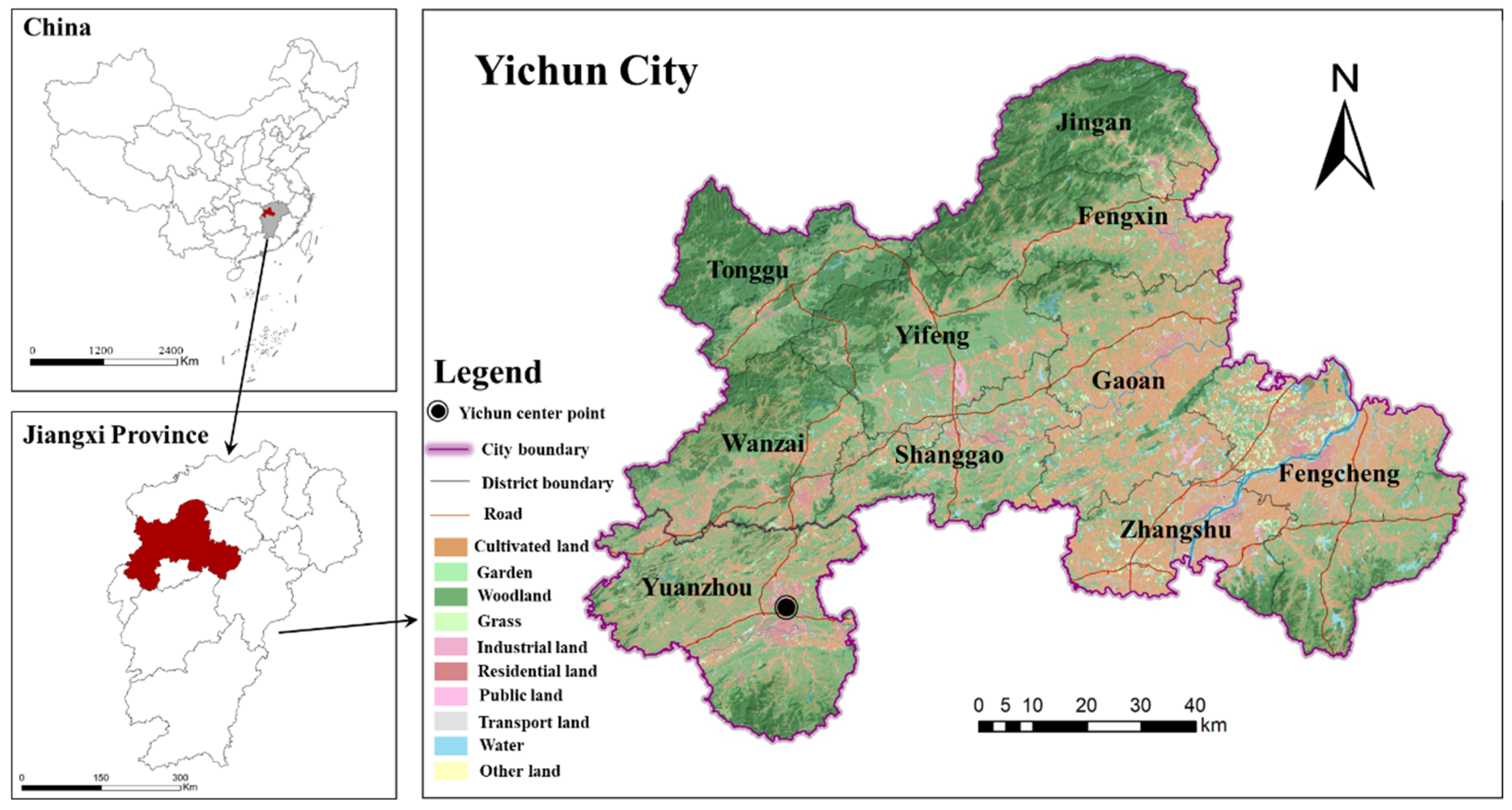
Yichun City, located at 27°33′–29°06′ N and 113°54′–116°27′ E, is the most remarkable tourist city of China in the northwest of Jiangxi Province (Figure 1). It covers 18,680.42 km², accounting for 11.2% of the total area of Jiangxi Province. It subordinates one district, six counties, and three county-level cities. Although the urban rate is continuously advancing, most areas of Yichun are rural areas. The altitude is between −137 m and 1771 m, with flat terrain and fertile soil. Therefore, the main types of land use in the rural areas of Yichun are cultivated land and rural residential land, covering 25.48% and 3.48% of the total territory, respectively.

With the urbanization and industrialization, rural Yichun has experienced economic stagnation and significant human–land relationship changes. From 2009 to 2018, the population of rural Yichun decreased from 4.3 million to 2.8 million, whereas the rural residential land expanded from 730.05 km² to 748.99 km². Of the cultivated land, 277 km² has been occupied by rural residential land during the aforementioned period. Rapid rural residential land expansion and cultivated land occupation in rural Yichun have damaged its agriculture development and natural ecosystems.

2.2. Data Source and Preprocessing

Multi-source data were integrated and utilized in the study, including (1) the second national land survey data in 2009 and 2018 obtained from the Yichun Natural Resources Bureau. According to the land use status classification (GB/T21010-2007), the patches with the land type code 203 were extracted from the database as rural residential land and the patches with the land type codes 0101, 0102, and 0103 as cultivated land. (2) Maps with a resolution of 30 m of population density and GDP in 2005 and 2015 were obtained from the geographic information monitoring platform (http://www.dsac.cn/, accessed on 1 January 2021). (3) Normalized difference vegetation index (NDVI) data were extracted from MODIS/Terra 250 m 16-day product MOD13Q1. (4) The data of rivers, roads, and other administrative centers were derived from the monitoring data of geographical conditions in Yichun. (5) Grain yield data in 2005 and 2015 were obtained from the Yichun Statistical Yearbook.

2.3. Flowchart of the Method

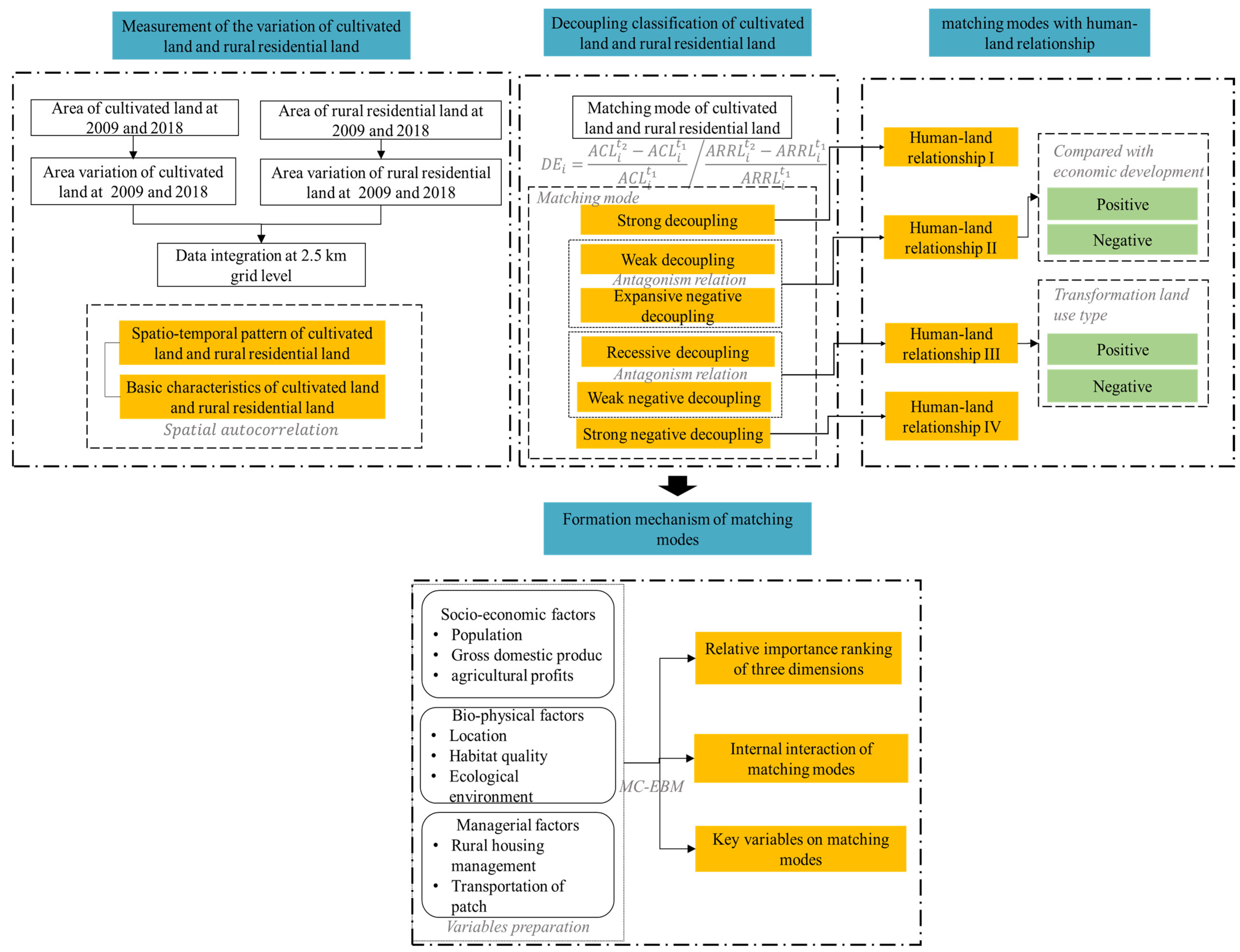
The integrated methods include four main components: measurement of the variation in cultivated land and rural residential land from 2009 to 2018, decoupling classification of matching modes between cultivated land and rural residential land, formation mechanism analysis of matching modes, and response strategies and corresponding relationship of matching modes with human–land relationship (Figure 2). The main steps of the method are as follows:

Step 1: We measured the variation in cultivated land and rural residential land from 2009 to 2018 at 2.5 km grid. Compared with other scales of grid, 2.5 km grid meets the needs of village construction and planning under the actual situation and status. The reason is that the area of 2.5 km grid is approximate to the average area of a village in Yichun.

Step 2: We divided the matching modes of variation in cultivated land and rural residential land from 2009 to 2018 into six types on the basis of the decoupling model.

Step 3: We constructed and quantified the influencing variables according to the formation mechanism system proposed by the existing studies. We then explored the formation mechanism of six matching modes.

Step 4: We defined the corresponding relationship between the various matching modes and coordination degree of human–land relationship and discussed the coordinated solutions of human–land relationship for guiding and establishing high-efficiency rural land use structure.

2.4. Decoupling Model

The coupling coordination degree model (CCDM) is applied to the coupling relationship between two factors in most existing studies, ignoring the relative change during land use transition. However, decoupling, originating from physics, is the mathematical separation of two systems and is helpful for evaluating the changes in the correlation between two systems. Carter [52] was the first to introduce decoupling into the economic and environmental fields and Tapio [53] further modified and improved it. The decoupling model was selected in this study to reveal the dynamic relationship between the change and conversion of cultivated land and rural residential land. Equation (1) is used to measure the decoupling relationship as follows:

$$D{E}_i=\frac{CL{T}_i}{RRL{T}_i}=\frac{AC{L}_i^{t_2}-AC{L}_i^{t_1}}{AC{L}_i^{t_1}}/\frac{ARR{L}_i^{t_2}-ARR{L}_i^{t_1}}{ARR{L}_i^{t_1}},$$

(1)

where $D{E}_i$ is the elasticity coefficient; $AC{L}_i^{t_1}$ and $AC{L}_i^{t_2}$ are the area of cultivated land of grid i at the period of $t_1$ and $t_2$, respectively; and $ARR{L}_i^{t_1}$ and $ARR{L}_i^{t_2}$ are the area of RRL of grid i at the period of $t_1$ and $t_2$, respectively. Through Tapio’s classification and other researchers’ perfections and applications with this model [54,55], six decoupling types are identified, and the details are provided in

Table 1. Decoupling classification of cultivated land change and rural residential land change.

Decoupling Type	$\mathit{C}{\mathit{T}}_{\mathit{i}}$	$\mathit{R}\mathit{R}\mathit{L}{\mathit{T}}_{\mathit{i}}$	$\mathit{D}{\mathit{E}}_{\mathit{i}}$	Decoupling Characteristics
Strong	≤0	>0	$D{E}_i$ ≤ 0	The cultivated land area decreases, whereas the rural residential land area increases.
Weak	>0	>0	$0 < D{E}_i$ < 1	Both cultivated land and rural residential land areas increase; the growth rate of the former is less than that of the latter.
Recessive	<0	<0	$D{E}_i$ ≥ 1	Both cultivated land and rural residential land areas decrease; the deceleration of the former is greater than that of the latter.
Expansive negative	>0	>0	$D{E}_i$ ≥ 1	Both cultivated land and rural residential land areas increase; the growth rate of the former is greater than that of the latter.
Weak negative	<0	<0	$0 < D{E}_i$ < 1	Both cultivated land and rural residential land areas decrease; the deceleration of the former is less than that of the latter.
Strong negative	≥0	<0	$D{E}_i$ ≤ 0	The cultivated land area increases, whereas the rural residential land area decreases.

.

2.5. Variables Preparation for MC-EBM Analysis

A certain consensus is reached regarding the formation variables of land use change, and these variables can be divided into socioeconomic, biophysical, and managerial dimensions [39]. Many studies are on the formation mechanism of cultivated land abandonment and rural residential land expansion, but the formation mechanism of the RCR attracts little academic attention and lacks quantitative analysis. This study therefore aims to deepen the understanding on it by quantifying the three dimensions mentioned above and referring to the specific variables selected by relevant studies.

Table 2. Description and calculation of variables.

Classification	Variable	Variable Description
Socioeconomic dimension	Gross domestic product (GDP)	GDP can measure the economic development status of a region in 2018. The GDP in a grid is ${\mathrm{GDP}}_i={\displaystyle \sum }GD{P}_{ij},$ $\mathrm{where} GD{P}_{ij}$ represents the value of grid j in the grid i.
	Gross domestic product variation (GDPV)	GDPV can measure the economic development status of a region from 2009 to 2018. The GDPV in a grid is ${\mathrm{GDPV}}_i=GD{P}_{i_{t_2}}-GD{P}_{i_{t_1}},$ $\mathrm{where} t_1$$\mathrm{and} t_2$ represent 2009 and 2018, respectively.
	Number of population (NP) [56,57]	NP can reflect the degree of population aggregation in a region. The NP in a grid is $N{P}_i={\displaystyle \sum }PO{P}_{ij},$ $\mathrm{where} PO{P}_{ij}$ represents the number of population of grid j in the grid i.
	Population variation (PV)	PV can measure the population migration of a region from 2009 to 2018. The PV in a grid is ${\mathrm{PV}}_i=N{P}_{i_{t_2}}-N{P}_{i_{t_1}},$ $\mathrm{where} t_1$$\mathrm{and} t_2$ represent 2009 and 2018, respectively.
	Average grain product per cultivated land (AGP) [58]	AGP is a vital variable to measure the ability of cultivated land produce in a region. The AGP in a grid is $AG{P}_i=\frac{G{P}_i}{AC{L}_i},$ $G{P}_i=G{P}_t\times \raisebox{1ex}{$VC{I}_i$}\!\left/ \!\raisebox{-1ex}{${\displaystyle \sum }VC{I}_i$}\right.,$ $VC{I}_i=\frac{NDV{I}_i-NDV{I}_{min}}{NDV{I}_{max}-NDV{I}_{min}}\times 100\%,$ $\mathrm{where} AC{L}_i$$\mathrm{represents} \mathrm{the} \mathrm{area} \mathrm{of} \mathrm{cultivated} \mathrm{land} \mathrm{in} \mathrm{the} i-\mathrm{th} \mathrm{grid}, G{P}_i$$\mathrm{represents} \mathrm{the} \mathrm{annual} \mathrm{grain} \mathrm{product} \mathrm{in} \mathrm{the} i-\mathrm{th} \mathrm{grid}, \mathrm{and} G{P}_t$$\mathrm{represents} \mathrm{the} \mathrm{total} \mathrm{value} \mathrm{of} \mathrm{annual} \mathrm{grain} \mathrm{product} \mathrm{in} \mathrm{the} \mathrm{region} t. NDV{I}_i$$\mathrm{represents} \mathrm{the} \mathrm{average} \mathrm{NDVI} \mathrm{value} \mathrm{of} \mathrm{grid} i, \mathrm{and} NDV{I}_{max}$$\mathrm{and} NDV{I}_{min}$ represents the maximum and minimum NDVI values of grid i.
Biophysical dimension	Habitat quality (HQ) [59,60]	HQ represents the impact of cultivated land and rural residential land changes on ecological environment. The HQ in a grid is $H{Q}_i=H_j\left\{D_x^2/(D_x^2+k^2)\right\},$ $\mathrm{where} H_j$$\mathrm{represents} \mathrm{the} \mathrm{habitat} \mathrm{suitability} \mathrm{score} \mathrm{for} \mathrm{land} \mathrm{use} j, D_x$ represents the total threat level in grid x with land use j, and k is the half-saturation constant.
	Distance to urban areas (DU) [57]	DU is the Euclidean distance to urban areas calculated by the kernel density value, which represents the location conditions of grid.
	Distance to the nearest county government site (DCG)	DCG is the Euclidean distance to county government site calculated by the kernel density value, which represents the location conditions of grid.
	Distance to the nearest township government site (DTG)	DTG is the Euclidean distance to township government site calculated by the kernel density value, which represents the location conditions of grid.
	Distance to river (DR) [61]	DR is the Euclidean distance to river calculated by the kernel density value, which represents the ecological environment of grid.
Managerial dimension	Patch density (PD) [62,63,64]	PD represents the rural residential land density, indirectly reflecting the distribution of rural residential land. The PD in a grid is $P{D}_i=\frac{N_i}{A{G}_i},$ $\mathrm{where} N_i$$\mathrm{represents} \mathrm{the} \mathrm{number} \mathrm{of} \mathrm{rural} \mathrm{residential} \mathrm{land} \mathrm{patches} \mathrm{in} \mathrm{the} \mathrm{grid} i, \mathrm{and} A{G}_i$ represents the area of grid i.
	Mean of perimeter area ratio (PARA_MN) [65]	PARA_MN is the perimeter irregularity extent of rural residential land patches, which represents the construction status of rural residential land.
	Distance to provincial roads (DP) [61]	DP is the Euclidean distance to provincial roads calculated by the kernel density value, which indirectly reflects the transportation status of grid.
	Distance to county road (DC) [61]	DC is the Euclidean distance to county road calculated by the kernel density value, which indirectly reflects the transportation status of grid.
	Distance to village road (DV) [61]	DV is the Euclidean distance to village road calculated by the kernel density value, which indirectly reflects the transportation status of grid.

describes and calculates the variables in detail.

In this study, we explore the antagonistic relationship between two matching modes (weak decoupling and expansive negative decoupling) by measuring the impact of two matching modes on socioeconomic level. We choose the area of main conversion types in the study period as independent variables, which are the conversion scale of cultivated land to garden land, forest land, grass land, industrial and mining storage land, rural residential land, and public management and service land to transportation land, water land, and unused land. We set the two matching modes (recessive decoupling and weak negative decoupling) as the binary dependent variables, arguing that the two matching modes are mainly affected by the above conversion types.

2.6. Multiclass Explainable Boosting Machine

MC-EBM stems from the generalized additive models (GAMs), which are the most powerful interpretable models, although it plays a pivotal role in individual features. Following the acceleration of interpretable models, Lou et al. [66] perfected and refined the GAMs through bagging and boosting, and their model is called the Explainable Boosting Machine (EBM) which is particularly suitable for the binary classification datasets. Previously, Zhang et al. [67] generalized EBMs to the multiclass setting, which is preferred in many real-world applications. This study assumes the multi-classification in which y = $\left\{1,2,\dots ,K\right\},$ K is the number of classes, the sample training set is $\mathrm{T}=\left(x_{n1},y_1\right),\left(x_{n2},y_2\right),\dots ,\left(x_{nd},y_n\right)$, and d is the feature. We aim to minimize the expected value of loss function $\mathrm{L}\left(\mathrm{y},\mathsf{\Theta }\left(\mathrm{x}\right)\right)$.

MC-EBM first considers standard GAMs with softmax probabilities and uses the multiclass cross entropy.

$$\stackrel{{\displaystyle ˇ}}{P\left(Y=k\right)=\frac{\exp \left(F_k\left(x\right)\right)}{{{\displaystyle \sum }}_{j=1}^K\exp \left(F_j\left(x\right)\right)}},$$

(2)

$$\mathrm{L}\left(\mathrm{y},\mathsf{\Theta }\left(\mathrm{x}\right)\right)=-{\displaystyle \sum }_k{1}_{y=k}log\widehat{\mathbb{P}}\left(Y=k\right),$$

(3)

where the logit of class k, $F_k\left(x\right)$, is also an additive function of individual features, $F_k\left(x\right)={\displaystyle \sum }_{i=1}^d{f}_{ik}\left(x_i\right)$; $f_{ik}$ is the shape function of feature i for class k; $\widehat{\mathbb{P}}\left(Y=k\right)$ is the model output, which is a probability distribution among the K classes; and $\mathsf{\Theta }\left(\mathrm{x}\right)$ represents the prediction of model on data point x.

Through cyclic gradient boosting, each boosting step fits a base learner to the pseudo-residual. The pseudo-residual for class j is as follows:

$${\tilde{y}}_j=-\frac{\partial L\left(y,{\left\{\widehat{\mathbb{P}}\left(Y=j\right)\right\}}_{j=1}^K\right)}{\partial F_j}=1_{y=j}-\widehat{\mathbb{P}}\left(Y=j\right),$$

(4)

In view of the problem of fitted base learner (multiplied by a typically small constant η), as suggested by Friedman et al. [68], MC-EBM takes an approximate Newton step using a diagonal approximation to the Hessian. The resulting additional update to learning multiple classes of GAM is

$$f_{ik}^{+}=f_{ik}+\eta {{\displaystyle \sum }}_l{\mathsf{{\rm Y}}}_{ilk}{1}_{x_iϵR_{il}},$$

(5)

$${\mathsf{{\rm Y}}}_{ilk}=\frac{K-1}{K}\frac{{{\displaystyle \sum }}_{x_iϵR_{il}}{\tilde{y}}_{jk}}{{{\displaystyle \sum }}_{x_iϵR_{il}}\left|{\tilde{y}}_{jk}\right|\left(1-\left|{\tilde{y}}_{jk}\right|\right)}$$

(6)

where $R_{il}$ is the set of training points in tree leaf l for current feature I. We follow the best hyperparameters for MC-EBM to be high performing: learning rate η = 0.01, number of leaves in tree L = 3.

3. Results

3.1. Spatio-Temporal Pattern of Cultivated Land and Rural Residential Land

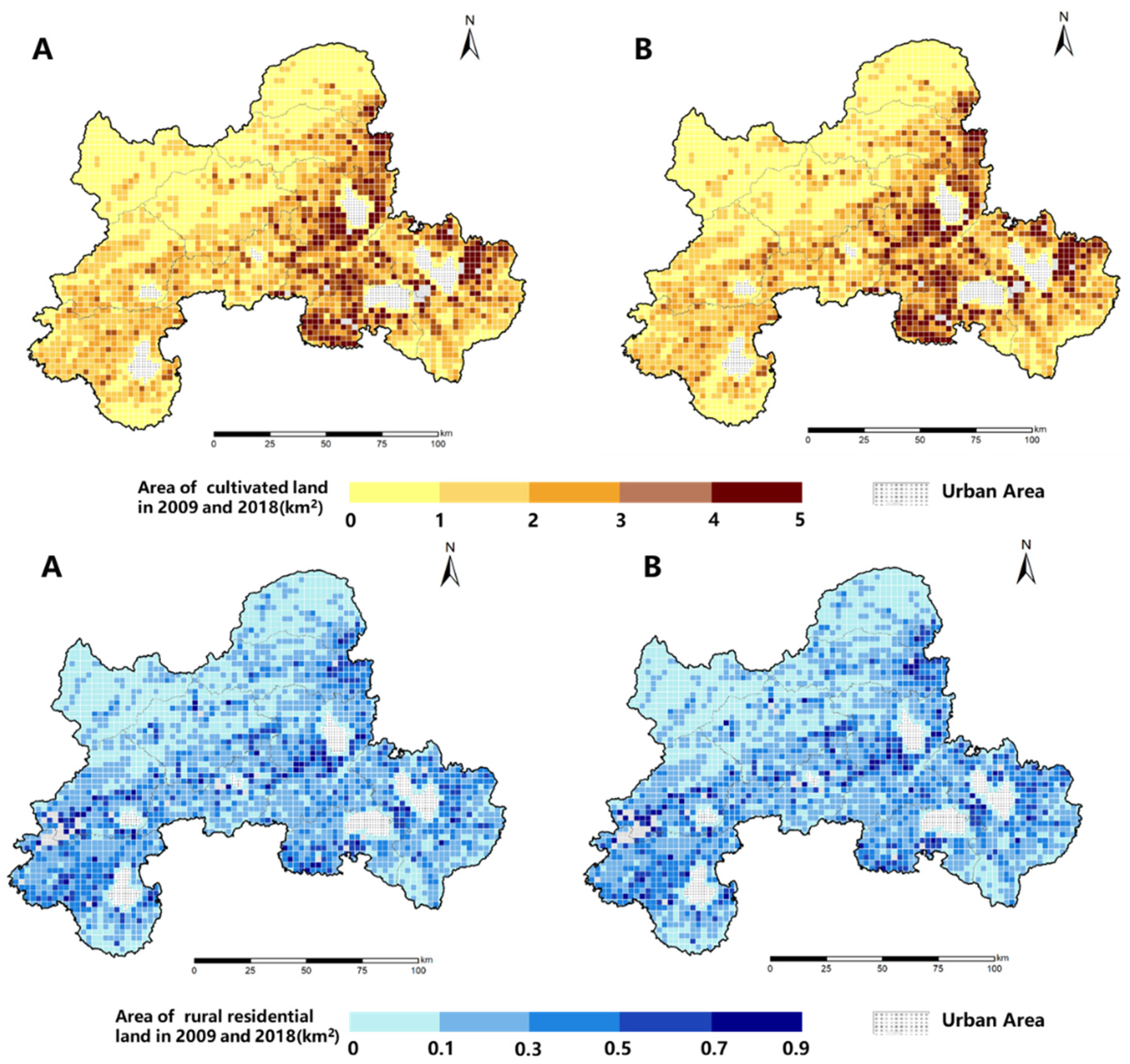
According to the analysis results, the cultivated land and rural residential land areas in Yichun were 46.87 ten thousand ha and 6.38 ten thousand ha in 2009 and 47.60 ten thousand ha and 6.50 ten thousand ha in 2018, respectively. The former decreased by 0.03 ten thousand ha, and the latter expanded by 0.12 ten thousand ha. Their spatio-temporal patterns are shown below.

The overall pattern of the cultivated land and rural residential land areas in 2009 and 2018 only slightly changed (Figure 3). For the cultivated land area, the high values were widely distributed in the plain areas or around urban areas, whereas the low values occupied the mountain areas. For the rural residential land area, the overall pattern was relatively scattered, mainly aggregated in the urban periphery and sparsely distributed in the mountain areas.

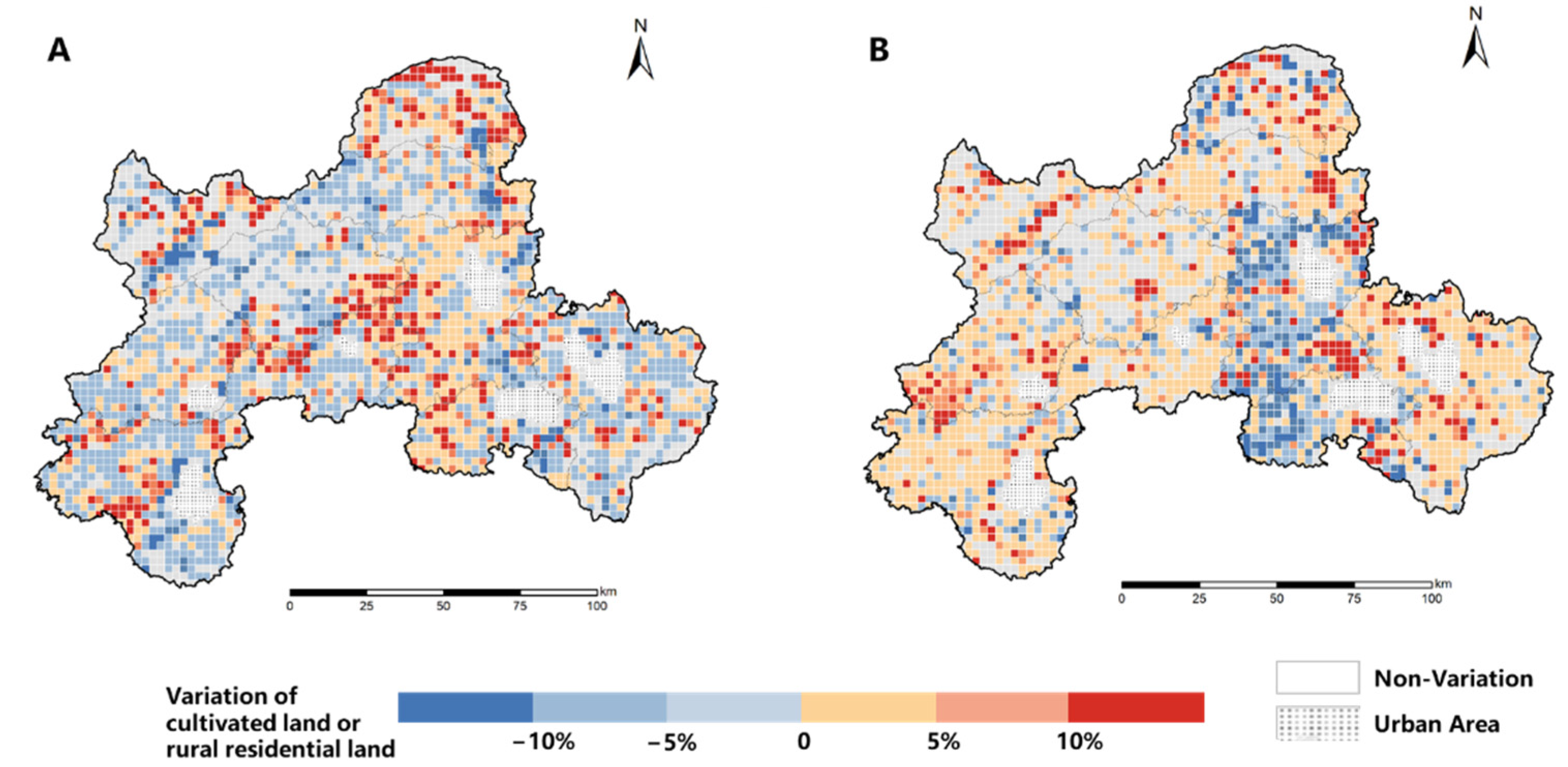
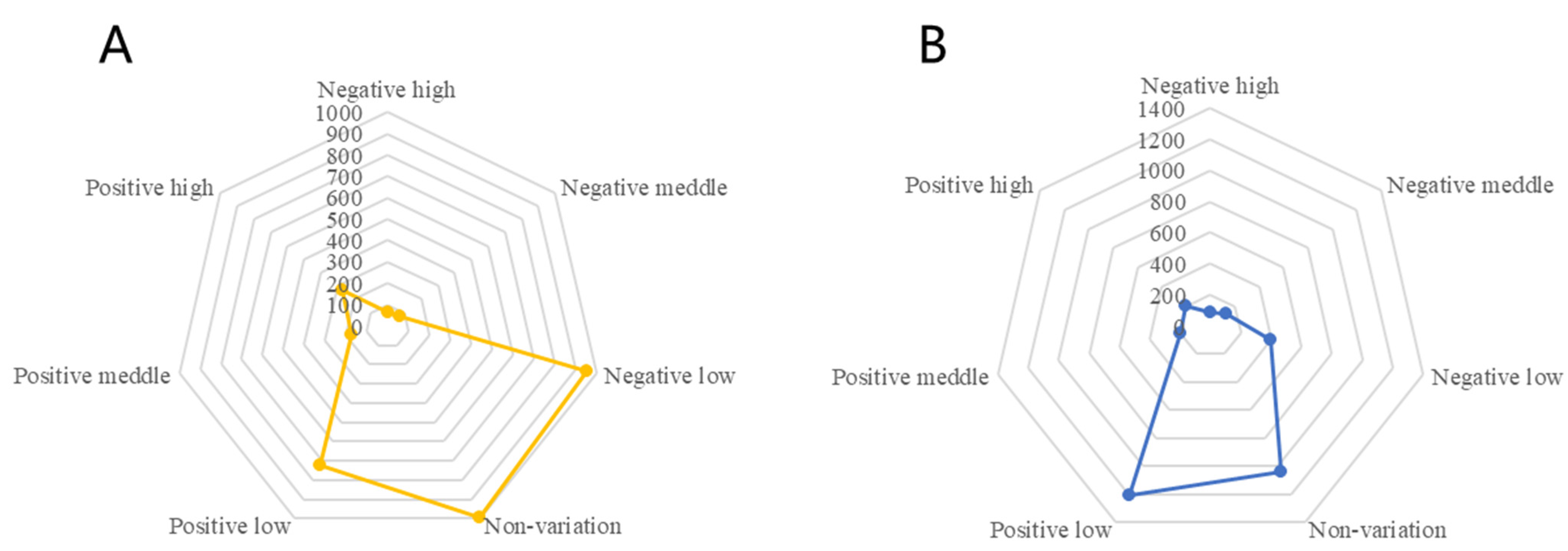
Figure 4 and Figure 5 and

Table 3. The proportion of matching modes distribution between 2009 and 2018.

Type	Negative High	Negative Middle	Negative Low	Non-Variation	Positive Low	Positive Middle	Positive High
Cultivated land	64	74	951	992	726	175	273
	1.97%	2.27%	29.22%	30.48%	22.30%	5.38%	8.39%
Rural residential land	86	129	397	1036	1208	195	204
	2.64%	3.96%	12.20%	31.83%	37.11%	5.99%	6.27%

show a substantial difference in the tendency of variation in cultivated land and rural residential land between 2009 and 2018. For cultivated land, the area variation was characterized by left-skewed distribution, illustrating that the proportion of negative low grids (29.22%) was greater than the positive low (22.30%). The total tendency of variation in cultivated land was decreasing. On the contrary, the variation in rural residential land was characterized by right-skewed distribution, illustrating that the proportion of positive low grids (37.11%) was greater than the positive low (12.20%). This result implied an increasing tendency of variation in rural residential land.

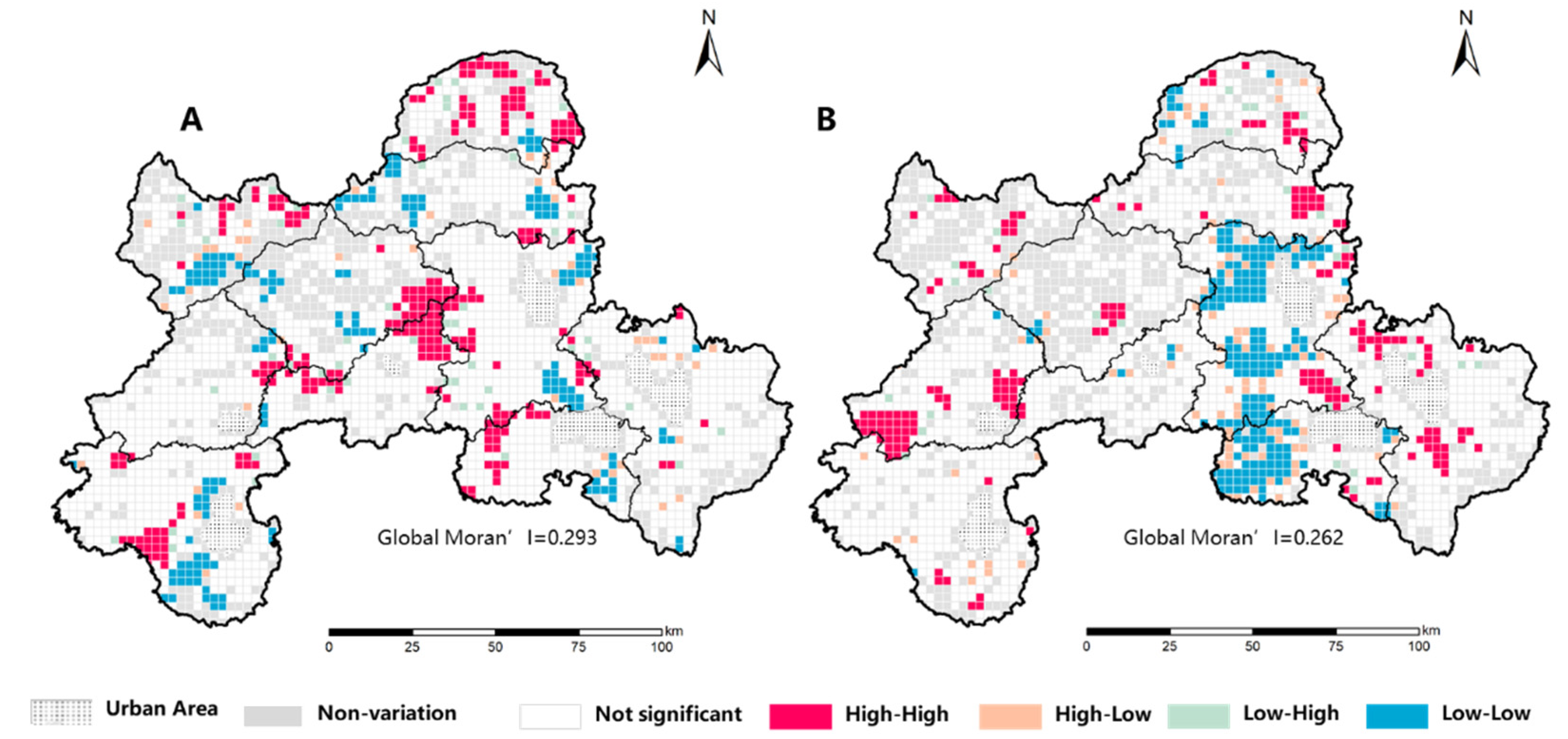
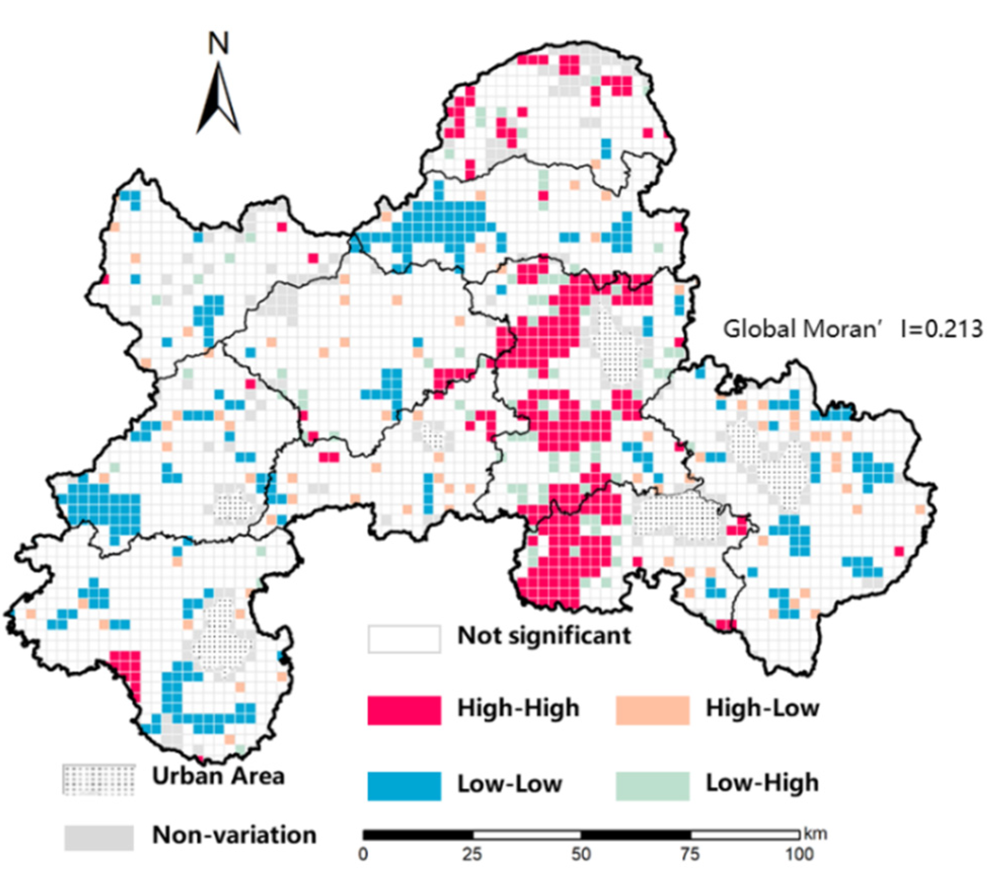
Figure 6 presents the spatial autocorrelations of variation in cultivated land or rural residential land from 2009 to 2018, identifying the hot and cold regions as well as spatial mismatch areas. Both Global Moran’s I index values of variation in cultivated land and rural residential land were significant and positive, with the index of variation in cultivated land (0.293) and variation in rural residential land (0.262). The result of spatial autocorrelations analysis showed the spatial mismatch of variation in cultivated land with rural residential land, which can be classified into four categories, namely, “cultivated land increased, whereas rural residential land decreased”, “cultivated land decreased, whereas rural residential land increased”, “cultivated land decreased along with rural residential land”, and “cultivated land increased along with rural residential land”.

3.2. Matching Modes of Cultivated Land and Rural Residential Land

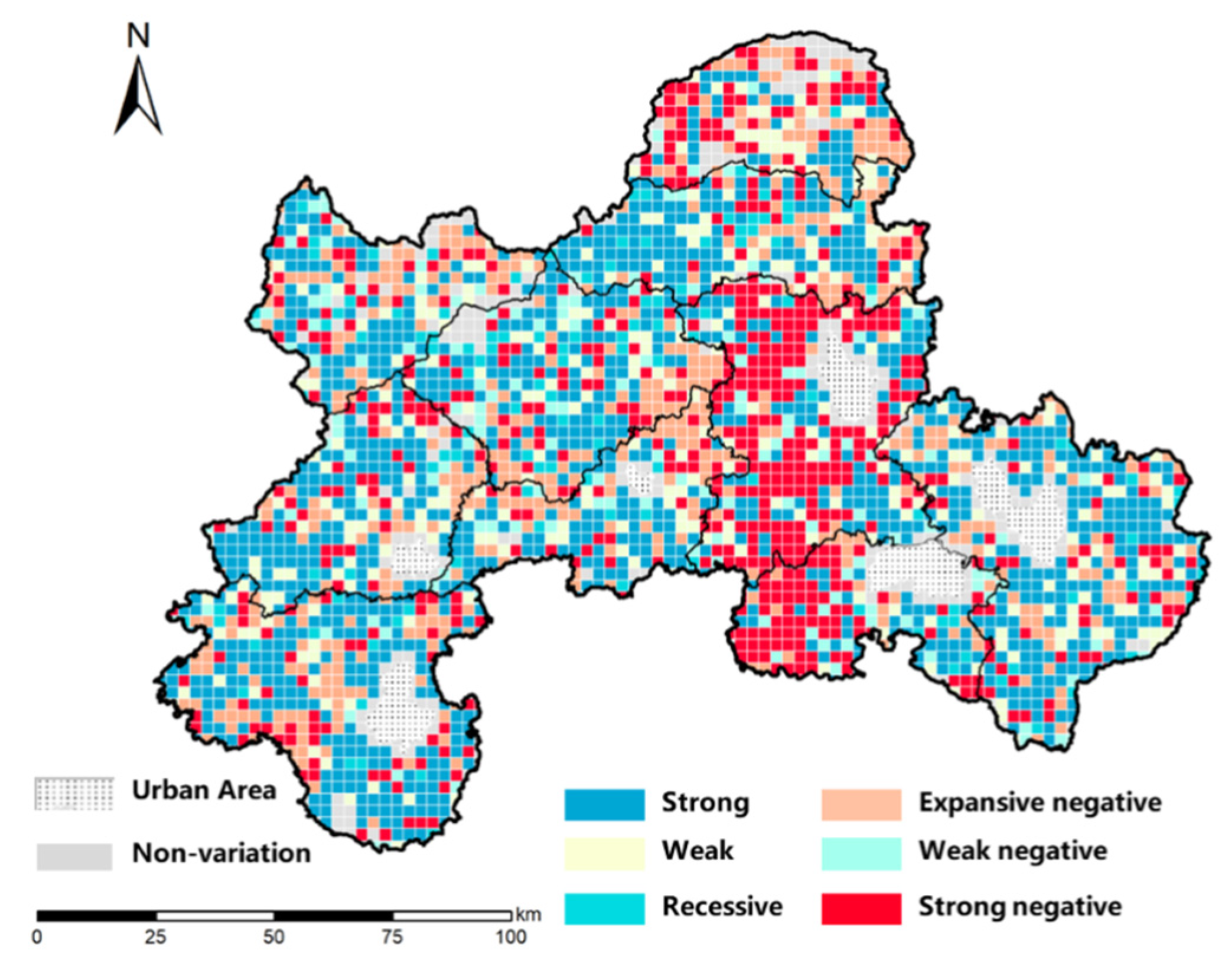
According to the analysis of spatial autocorrelation, the phenomenon of spatial mismatch between cultivated land and rural residential land was found. However, to what extent and to where was the unbalanced distribution of cultivated land and rural residential land remained unclear. The decoupling model further analyzed the changes in cultivated land and rural residential land, comprehensively identifying and orienting the matching modes between the two. The results indicated six types, namely, strong decoupling (SD) (33.36%), weak decoupling (9.86%), recessive decoupling (4.15%), expansive negative decoupling (15.05%), weak negative decoupling (4.92%), and strong negative decoupling (SND) (18.65%). Among them, the SD and strong negative decoupling were the most dominant matching modes, with others the transition modes.

SD: The type represented a decrease in the area of cultivated land and an increase in the area of rural residential land. It was the most substantial type among the six matching modes, accounting for 33.36% in 3225 grids. As shown in Figure 7 and Figure 8, the strong decoupling was disorderly scattered in Yichun, showing that the unbalanced RCR emerged as a prevalent phenomenon. It was disadvantaged by its rural population seasonal migration and resulted in cultivated land abandonment and rural residential land expansion.

Weak decoupling and expansive negative decoupling (WED): These two types represented a synchronous increase in cultivated land and rural residential land, respectively, accounting for 9.86% and 15.05%. They both showed favorable agricultural development momentum along with the issue of rural residential land occupying other land use, such as forest in this region. Weak decoupling implied that the area growth speed of cultivated land was less than rural residential land; that is, the agricultural development was weaker than that of the rural residential land expansion. By contrast, expansive negative decoupling implied that the area growth speed of cultivated land was greater than rural residential land, revealing that the agricultural development was stronger. The impact of these two matching modes on socioeconomic level should be verified.

Recessive decoupling and weak negative decoupling (RWD): Recessive decoupling and weak negative decoupling were the subsidiary types. The former referred to a synchronous decrease in cultivated land and rural residential land reaching 4.15%, indicating that the area deceleration speed of cultivated land was greater than rural residential land. Weak negative decoupling was similar to recessive decoupling, but the area deceleration speed of cultivated land was less than rural residential land, reaching 4.92%. They all carried out effective rural residential land consolidation, but what kind of land cultivated land has been transformed into needed further discussion.

SND: This was the best and most ideal mode for the matching condition of cultivated land and rural residential land in Yichun among the six types, accounting for 18.65%. As shown in Figure 7 and Figure 8, the SND presented the spatial gathering in the middle. As shown in

Table 4. Terrain and matching modes distribution in Yichun.

Terrain	Strong	Weak	Recessive	Expansive Negative	Weak Negative	Strong Negative
Plain	10.20%	3.41%	0.80%	4.85%	1.63%	8.17%
Hill	10.20%	2.92%	1.29%	5.93%	1.01%	4.39%
Mountain	12.96%	3.53%	2.06%	4.27%	2.27%	6.08%
Sum	33.36%	9.86%	4.15%	15.05%	4.92%	18.65%

, the SND was more sensitive to terrain than other types, revealing that its proportion increased by 3.78%, from 4.39% in the hill to 8.17% in the plain, whereas those of the other types merely floated by 1%. In this region, the rural residential land consolidation was smoothly pushed forward, with the booming rise of agriculture.

3.3. Key Variables on Matching Modes

Based on the classification results, we chose the MC-EBM model to further analyze their formation mechanism. Notably, as the matching condition of WED and RWD was consistent, we combined them into a single mode. We then discussed the antagonistic relationship of the former pattern with economic development and what kind of land use type the cultivated land transformed into in the latter pattern. Partial dependence plots (PDPs) were used to visualize the marginal effects of the variables on the predicted outcomes holding all other variables constant. The ladder diagram was selected to avoid the excessive fluctuation of the curve. We also estimated the multiclass logistic regression (MLR) model and selected SD as the base class for the universality. The model was significant with a confidence level of 0.05, indicating that it was valid. The predictive accuracy (0.455) was lower than that of the MC-EBM model (0.578) owing to the non-linear effects, which can promote the overall goodness of fit.

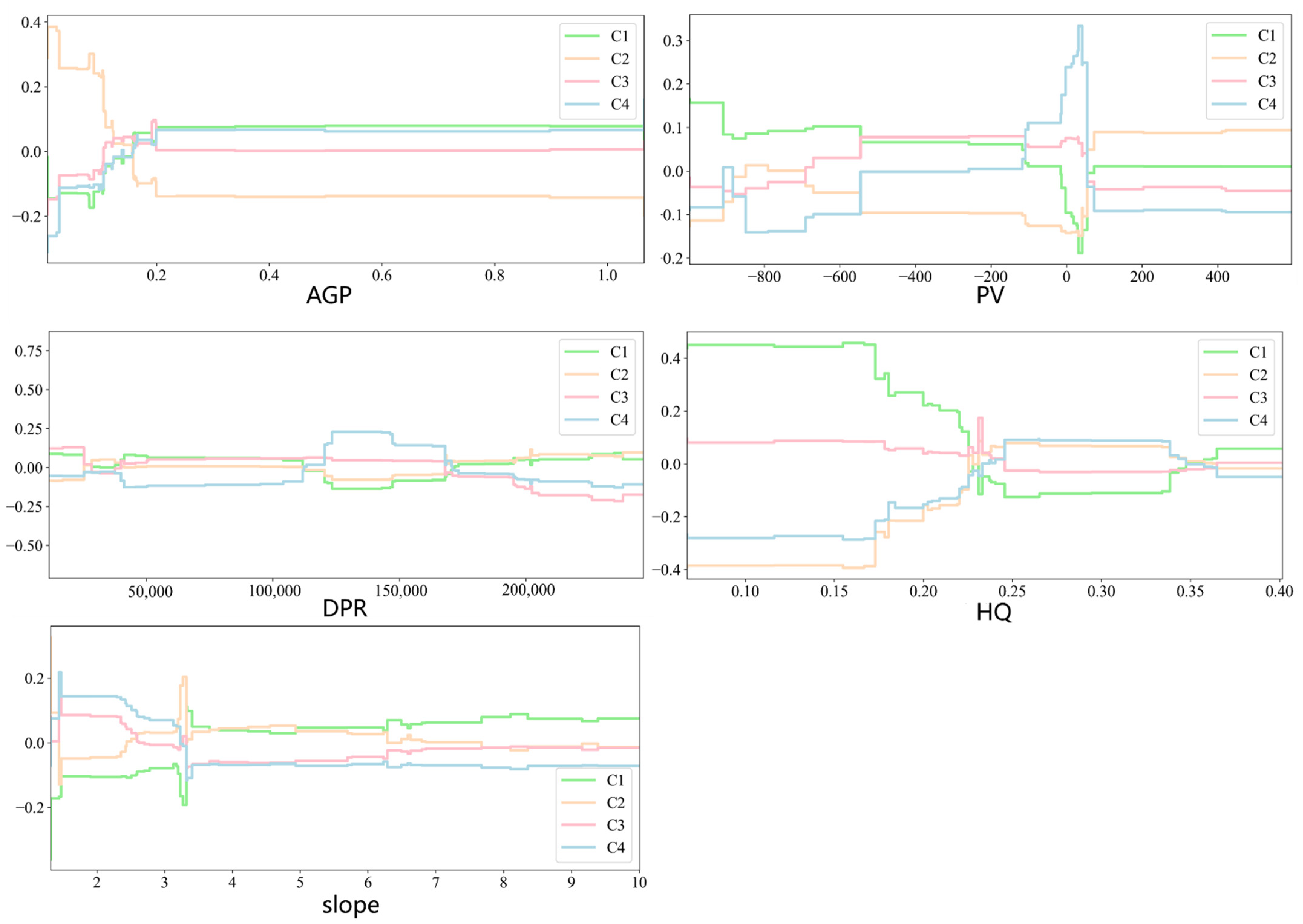
In terms of the relative importance ranking, AGP, PV, DPR, HQ, and slope were the top five key variables with significant effects on the matching modes. According to the average relative importance of three dimensions, the descending order was biophysical dimension (5.49%), socioeconomic dimension (5.38%), and managerial dimension (3.29%). PDPs were composed of different line types, with the y axis representing the occurring probability of four matching modes. In terms of the floating tendency of four curves, we found that the line “SD” was often along with the line “RWD” and that the line “WED” was often along with the line “SND.”

As illustrated in Figure 9, AGP was the most important variable, and it positively affected the formation of matching cultivated land and rural residential land. Its value and the probability of SND were higher. PV was the second most important variable with the strongest impact on the matching modes. It was the key variable to determine whether the matching mode of cultivated land and rural residential land was reasonable or not. The probability of each matching mode largely fluctuated at the threshold where the PV was −108 and 0. When the value of PV was less than −108, SD was most likely to occur, indicating that SD tended to accompany population decrease. When the value of PV was at the range of −108 to 0, the probability of SND gradually increased to the maximum, indicating that the population variation in SND was reasonable. When the value of PV was greater than 0, WED was the dominant decoupling type, followed by SD, indicating that the variation in rural residential land in WED and SD was also reasonable. That is, PV had a non-linear relationship with SD, which meant a high probability of SD when the population increased or decreased to a certain value. According to DPR, the influence on the matching modes manifested gradient characteristics along the transect “SD-disorder-SND-SD/RWD”. As for HQ, SD likely occurred when the value of HQ was excessively high or low, which meant that HQ also had a non-linear relationship with SD. As the slope gradually steepened, we observed the rapidly increased probability of SD and RWD. To be precise, the slope was greater than 6° (classified as gentle slope). When the slope was large, SD could be converted to RWD. Similarly, when it was below the threshold of 6° (classified as flat slope), it was more likely to appear as SND or WED.

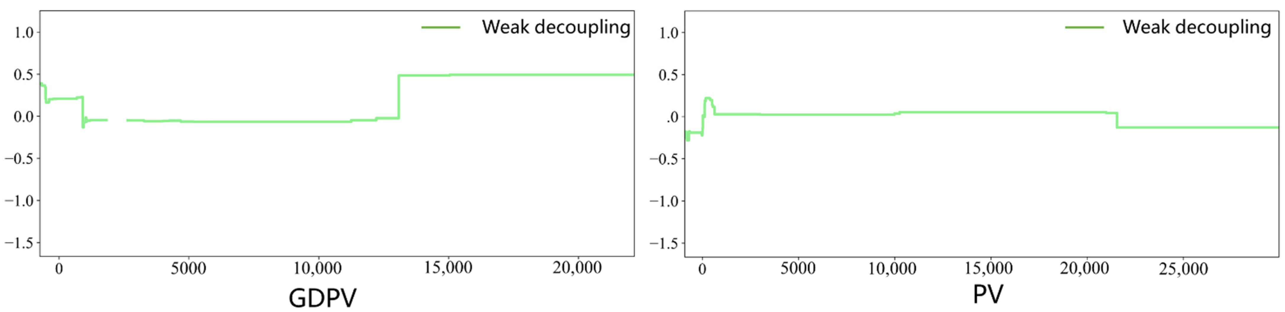
Although the WED inevitably caused serious problems in the economic development, how did its antagonistic relationship affect economic development? We compared the WED with GDPV and PV, which refer to economic development. Overall, weak decoupling imposed the better performance on economic development; that is, when the value of GDPV and PV was high and positive, weak decoupling likely occurred (all variations are shown in Figure 10).

The whereabouts of cultivated land loss in the RWD remained unclear, and it is of great significance for exploring what kind of land is occupying cultivated land. We quantitatively evaluated the transition of cultivated land to other land use types from 2009 to 2018 and discussed the relative importance influencing the formation of RWD by using the MC-EBM model. As shown in

Table 5. Results of variable relative importance on the formation of RWD.

Variables	Relative Importance (%)	Rank
Cultivated land to forest land (CL2FL)	21.01	1
Cultivated land to transportation land (CL2TL)	12.84	2
Cultivated land to rural residential land (CL2RL)	11.01	3
Cultivated land to water land (CL2WL)	10.79	4
Cultivated land to public management and service land (CL2PL)	7.14	5
Cultivated land to unused land (CL2UL)	6.21	6
Cultivated land to grass land (CL2GL)	5.42	7
Cultivated land to garden land (CL2G)	4.76	8
Cultivated land to industrial and mining storage land (CL2IL)	3.12	9

, forest land, transportation land and rural residential land were the three land use types that occupied cultivated land.

4. Discussion

This study adapted a grid-based integrated decoupling model and MC-EBM analysis method to analyze the matching modes of RCR, which fully meet the needs of village–town construction and are conducive to the precise type and location of RCR. The results of this study enabled us to provide theoretical guidance on improving rural human–land relationships, assessing land use structure scientifically, optimizing the allocation and utilization of cultivated land and rural residential land, and promoting sustainable rural agriculture development in Yichun.

4.1. Basic Characteristics of Cultivated Land and Rural Residential Land

In this study, we found a substantial difference in the cultivated land and rural residential land from the perspective of area variation tendency from 2009 to 2018. From the perspective of the total area overall pattern, only a slight change was noted. For the cultivated land, the area variation was characterized by left-skewed distribution, which indicated that the total tendency of cultivated land was decreasing. On the contrary, the variation in rural residential land was characterized by right-skewed distribution, implying an increasing tendency of rural residential land. These results showed that the variation between cultivated land and rural residential land was characterized by quantity match, which was in line with the findings from previous studies [33,51]. As most cultivated land is highly productive and well concentrated, the seasonal migrants returning to their hometowns to build houses are inclined to occupy cultivated land, which resulted in the quantity match of variation in cultivated land and rural residential land, verifying a change in the RCR [39,40].

The results of spatial autocorrelations analysis indicated that the spatial mismatch of variation in cultivated land and rural residential land made the SD in six matching modes more remarkable. Rural land consolidation should adopt the corresponding response strategies and chronological sequence based on the disparate decoupling type [40,61]. In general, the four main types of the matching modes corresponding to the decoupling results are “cultivated land increased, whereas rural residential land decreased” (SD), “cultivated land decreased, whereas rural residential land increased” (SND), “cultivated land decreased along with rural residential land” (RWD), and “cultivated land increased along with rural residential land” WED.

4.2. Formation Mechanism of Matching Modes

This study quantitatively analyzes the impact of socioeconomic factors, biophysical conditions, and managerial factors on the matching modes with the aid of the MC-EBM model at grid unit. In comparison with other studies, we determine the formation mechanism of six matching modes based on the ranking of the collective relative importance of three factors with the aid of the MC-EBM model. The six matching modes of cultivated land and rural residential land are the results of socioeconomic factors and managerial factors based on the biophysical conditions. The biophysical conditions have a long-lasting influence on the matching modes, which lay a basic foundation for the change direction of cultivated land and rural residential land. Against this foundation, the socioeconomic factors determine the final change direction. The managerial factors correct the matching modes and can be used as the direct solutions to improve the uncoordinated matching modes.

First, the biophysical conditions lay a basic foundation for the change direction of cultivated land and rural residential land. According to the MC-EBM analysis, the biophysical conditions within the grid determine the quality of cultivated land, and the change direction of cultivated land further determine the change direction of rural residential land. In the areas with large slope and good habitat quality, which are generally the mountain areas, the fragile ecological environment is not suitable for farming. As a result, cultivated land gradually degrades, and rural residential land tends to occupy the little high-quality cultivated land suitable for living, resulting in a contradictory pattern of decreasing cultivated land and increasing rural residential land. This finding is consistent with most conclusions on cultivated land abandonment and rural residential land transfer in mountainous areas [13,33]. In terms of the non-linear results of HQ and DPR, the explanations are as follows. For HQ, the emerging of SD may be attributable to cultivated land occupying the ecological rural land in the plain or hill where the value of HQ was low. Conversely, when SD occurred in mountainous areas, the value of HQ remained high, which was likely due to its intrinsic high HQ [60]. For DPR, the performance of SD manifested the multilayer change, and this finding is in line with those of the existing studies [61]. Specifically, in areas far away from urban ones, the rural population tend to be attracted to urban areas by the developed economic conditions, so the cultivated land is left uncultivated [3]. At the same time, seasonal migrants with higher incomes who return home to build new houses further occupy idle cultivated land, resulting in the contradiction of cultivated land and rural residential land. The areas around the administrative centers expand mainly by absorbing surplus rural labors, which led to the increase in rural residential land. The decrease in cultivated land may be due to the preference of the surrounding areas for non-agricultural and urbanization-led development [69].

The final change direction of cultivated land and rural residential land is determined by the socioeconomic factors, conforming to the hypothesis. In all dimensions, AGP and PV have the highest relative importance and play the greatest role in determining the type of matching modes, which also demonstrate that the matching modes are highly correlated with the coordination degree of the human–land relationship. That is, the cultivated land marginalization with low AGP contributes to cultivated land abandonment essentially and the population variation with negative PV jointly contributes to unbalanced matching modes. The continually declining cultivated land profits and the rapid and mass migration of the rural population are the key causes of low efficiency in rural land use structure. The results showed that AGP has a positive effect on the formation of SND, which is in line with the findings of the previous studies [64]. Notably, PV has non-linear relationship with the most unbalanced and widespread matching mode (SD). Undoubtedly, when the rural population lost too much, hollowed village and SD formed, which resulted in the peripheral expansion and internal idleness of rural residential land and abandonment of cultivated land [70]. Despite the rural population growth, WED can be easily transformed to SD if the management of newly built rural residential land is neglected. This is because the newly built rural residential land tends to be built in the well terrain and convenient location conditions, and these areas are often cultivated land [50].

Finally, the managerial factors correct the result of matching modes and can be used as the direct solutions to improve the unbalanced matching modes. The MC-EBM analysis shows that the transportation conditions positively affect the formation of SD. Newly built rural residential land was along the road, eventually creating the phenomenon of “housing along the road” on what used to be cultivated land [71].

In comparison with other studies, this study further discusses the internal interaction of matching modes. We adopt the MC-EBM model, an interpretable model which has broken the limitation that most models is less transparent and could explore the potential relationships among matching modes. A concomitant phenomenon is found in the matching modes, referring to the SD that occurred with the RWD and the WED that occurred with the SND in the same conditions. Compared with the cultivated land, the rural residential land consolidation projects are more effectively implemented, and they have achieved great success in rural areas [24,40]. This result can be considered in the partition strategy and help orderly improve the matching modes of cultivated land and rural residential land.

4.3. Corresponding Relationship and Response Strategies Based on Matching Modes and Human–Land Relationships

Due to the interpretability and transparency of MC-EBM, we could observe the occurrence probability of matching modes with the variation in influencing factors. Therefore, we followed the model results of six matching modes and four dominant human–land relationships in different grids. Combining the MC-EBM results of influencing factors, we discussed the corresponding relationship and strategies of matching modes and human–land relationships from the viewpoint of guiding and establishing the high-efficiency rural land use structure and coordinated development of human–land relationships.

Among all matching modes, SD is the most common type, which reveals the first level of human–land relationship. This type represents a contradiction between the cultivated land and rural residential land in the region (the decreased cultivated land and increased rural residential land). In this region, the AGP is generally low, which implies the low mechanization, serious marginalization, and fragmentation of cultivated land and the non-agricultural transition. The population migration will also increase the risk of cultivated land abandonment due to the non-agricultural transition. With the promoting of non-agricultural employment level, growing income and improving living standards will further induce the phenomenon of abandoning original rural residential land. As the PV is negative and the population loss is widespread in the region, this type also represents the uncoordinated human–land relationship between decreased population and increased rural residential land. Hence, the key to improve the human–land relationship in this region is to promote the agriculture profits, control the floating population, and attract the population to return. According to the MC-BEM analysis, the occurrence probability of SD and RWD often presents a concomitant phenomenon, so guiding SD to develop into RWD first can be considered. That is, idle rural housing land consolidation should be first promoted and the rural residential land paid exit mechanism should be established to gradually decrease rural residential land and reduce the inefficient occupation of cultivated land. Generally, this region frequently emerges in the urban suburbs or the mountain areas, with the biophysical conditions of steep landforms (slop greater than 6°), extreme ecological service levels, and far from or close to urban areas. For urban suburbs, compared with the high level of social and economic development and the advanced extent of urbanization and industrialization, the region exits prominent contradiction between cultivated land and urban construction land. Therefore, during urbanization, high-quality cultivated land should be strictly guaranteed, for instance, improving the degree of mechanization, avoiding the cultivated land fragmentation, and strengthening the intensive use of cultivated land [40]. When the region enters the maturity stage of hollowing with the continuous idle of rural residential land, the “urbanization leading model” should be adopted for rural residential land consolidation to avoid occupying urban and rural land resources [61]. For the mountain areas, the main problem of this region is the fragile ecological environment. The ecologically sensitive areas in this region should be marked as ecological land and used for grain-for-green and rural land consolidation programs, and the existing cultivated land and rural residential land should be gradually restored to ecological land [51]. Moreover, this region should strengthen the construction of sloping cultivated land and improve the cultivated land marginalization in the suitable farming areas [36].

WED is the second level of human–land relationship, which represents a synchronous increase in cultivated land and rural residential land. In this region, the PV is positive, and the population is gradually increasing. Therefore, this type also represents the booming-development human–land relationship between increased population and increased rural residential land. It has a great potential for rural development, especially the agriculture development in this region. Hence, with the increasing cultivated land, the productivity and utilization efficiency of cultivated land should be paid attention to, avoiding the fragmentation and marginalization of the cultivated land and adhering to ecological red lines, to realize the simultaneous promotion of quantity and quality of cultivated land [11,40]. However, in the face of rural residential land expansion and increasing rural population, the region urgently needs to carry out rural housing consolidation, especially saving and intensifying rural housing land use [72]. In the antagonistic relationship in the WED, the victory of weak decoupling is conducive to the realization of rural population and economic sustainable development. It is reasonable, since industry, especially agriculture, is the cornerstone of rural development. Compared with expansive negative decoupling, weak decoupling plays a relative positive role in economic growth.

RWD is the third level of human–land relationship, which represents a synchronous decrease in cultivated land and rural residential land. In this region, the PV is little, and the population variation is stable. Therefore, this type represents the gradually steady human–land relationship between stable population and decreasing rural residential land. Population and rural residential land reflect a benign interaction in this region, and the matter warranting concern in this region is the cultivated land transition. Cultivated land is invaded by other land use types except rural residential land. According to the MC-BEM analysis, forest land is the major land use type of cultivated land transition, and new land should be given priority to forestry [40]. Transportation land is the second land use type of cultivated land transition, likely causing cultivated land fragmentation and bringing many adverse consequences to the rural agriculture sustainable development. Therefore, the encroachment of cultivated land for transportation should be prohibited in village-town planning [73]. Although rural residential land shows a declining trend, the phenomenon of rural residential land occupying cultivated land remains serious, which is the third land use type of cultivated land transition. The management of newly built housing must be strengthened, especially the cultivated land with better location conditions [74].

SND is the fourth level of human–land relationship, which represents an ideal condition of the change in cultivated land and rural residential land. In this region, the PV is not significant, and the population variation is stable. Therefore, this type represents the steady human–land relationship between stable population and decreasing rural residential land. SND represents a benign interaction between population and rural residential land and between cultivated land and rural residential land. In the region, population loss is not significant, habitat quality is less affected by human activities, and land management is in place.

The MC-EBM model is extensively applied to the transportation field, which aims to solve the multiple classification problem. This study firstly applies the method in the field of land use, which could visualize the formation mechanism and internal interaction of RCR. It provides an important starting point from qualifying and generalizing the formation mechanism of land use change to quantitative analysis. However, due to the limitation of data source, we can only propose the aim of application and implementation in the spatial planning, and how to apply in practice requires further exploration in the subsequent studies.

5. Conclusions

This study aims to quantitatively characterize the matching modes of cultivated land and rural residential land, the underlying formation mechanism, via a grid-based integrated decoupling model and MC-EBM analysis method. The conclusions are as follows. (1) The basic characteristics of cultivated land and rural residential land are identified. A substantial difference is noted in the cultivated land and rural residential land from the perspective of the area variation tendency from 2009 to 2018. The variation in cultivated land and rural residential land was characterized by quantity match and spatial mismatch. (2) Their underlying formation mechanism is found. That is, their matching modes are the result of socioeconomic and managerial factors based on the biophysical conditions. The prediction accuracy of the MV-EBM model is higher than that of multiple linear regression model. Specifically, AGP, PV, DPR, HQ, and slope are the top five key variables that have significant effects on the matching modes. A concomitant phenomenon is noted in the matching modes, referring to the SD that occurred with the RWD and the WED that occurred with the SND in the same conditions. (3) A significant corresponding relationship exists between the matching modes and the human–land relationship, indicating that the six matching modes correspond to four different stages of human–land relationships. Particularly, in terms of the land use type wherein the loss of cultivated land transferred in the RWD, forest land was positive, whereas rural residential land and transportation land were negative. Overall, the findings are of great significance to formulate differentiated cultivated land and rural residential land management policies. They also provide a theoretical basis for implementing the rural revitalization strategy and coordinating human–land relationships. However, the method is needed to fully tape the application potential in the usage of spatial planning.