Exploring the Effects of Transportation Supply on Mixed Land-Use at the Parcel Level

Abstract

The interactive relationship between transportation and land use has become more difficult to understand and predict, due to the economic boom and corresponding fast-paced proliferation of private transportation and land-development activities. A lack of coordination between transportation and land-use planning has created an imbalanced provision of transportation infrastructure and land-use patterns; this is indicated by places where a high-density land-development pattern is supported by a low-capacity transport system or vice versa. With this, literature suggests that Mixed Land-Use (MLU) developments have the potential to provide relevant solutions for urban sustainability, smart growth, inclusive public transit use, and efficient land-use. Therefore, this study employed deep neural network models—Long Short-Term Memory (LSTM), and Multilayer Perceptron (MLP)—for forecasting the effect of transportation supply on the MLU pattern at the parcel level in the Jiang’an District, Wuhan, China. The findings revealed a strong relationship between the supply of public transportation and MLU. Moreover, the study results indicated that MLU is widely available in areas with high accessibility, high density, and proximity to the city center. The forecasting results from the MLP and LSTM models showed an average error of 5.55–7.36% and 3.62–4.28% for mixed use, respectively, while most of their 90th percentile errors were less than 13.73% and 10.46% for mixed use, respectively. The proposed models and the findings from this study should be useful for stakeholders and policy makers for more precise forecasting of MLU at the urban level.

1. Introduction

Mixed land-use (MLU) is a modern planning paradigm that enables compatible land used for various socioeconomic activities to be located in close proximity to each other, thereby reducing the travel distance/time between them. MLU refers to a range of functional land-uses, including residential, commercial, industrial, institutional, and transportation-related. It has been promoted as a significant component of modern urban development strategies, such as smart growth, Transit-Oriented Development (TOD), walkability, and compact development [1,2,3,4]. MLU is expected to provide numerous social benefits such as urban vitality, social cohesiveness, job generation, and efficient use of public utilities, and reduce travel distance, energy consumption, and CO₂ emissions [5]. MLU is essential for the sustainable development of large and medium-sized cities. Cities in Europe are often featured with mixed land-use areas that are efficiently connected via public transportation. In addition, it is evident from the literature that households and apartment dwellers are more willing to pay for a house in a mixed neighborhood with business services and entertainment than for a house in a segregated-land-use area [6]. Meanwhile, fast economic development, urbanization, and motorization have resulted in various negative impacts, such as traffic congestion, accidents, and air pollution [7,8]. On the other hand, urban sprawl with low land-use density mostly relies on private cars for travel, leading to traffic congestion and high travel costs [9]. Similarly, large and medium-sized cities are vigorously promoting the development of subway and ground bus networks [10,11]. Thus, land-use and transportation planners should have a thorough understanding of the dynamic connections between urban form, land-use patterns, and transportation supply. Experiences from many cities around the globe indicate that they must integrate land-use and transportation planning because the alteration of one of the two affects the other, and cities or areas with an uncoordinated land use and transportation supply are much less sustainable. Planners are unable to perform a strategic intervention to attain the desired urban shape unless they have a thorough understanding of the dynamic linkages between the two systems [12]. There is a strong association between the urban form, accessibility, and other variables such as activity distribution, employment, and land-use patterns [13]. A previous study by Jayasinghe et al. [14] shows that high-accessibility areas tend to have a high mixed-land-use density, whereas low accessibility areas have low mixed-land-use density.

TOD is a compact, mixed-use development close to transit amenities that provides a better environment for walking and cycling. It consists of office space, new residential development, and other service facilities that are within a half-mile of public transit and are easily accessible via walking or bicycle. TOD usually promotes sustainable communities by providing an inexpensive, convenient, and physically active style of living. TOD focuses on developing integrated communities with commercial clusters and recreation centers to prevent urban sprawl. The key advantages of TOD include an increase in land values, increased higher-density development, the promotion of active transportation, the improvement of business visibility, and the introduction of new prime retail areas to attract customers to businesses [15]. Transportation primarily facilitates accessibility and mobility. Accessibility refers to people’s ability to access products, services, and activities, which is the primary objective of most transport activities. In addition, accessibility reflects the influence of land-use distribution and transportation system characteristics on user access. Therefore, land use and transportation are related because they allow people to participate in activities occurring in different locations [16,17]. Moreover, numerous studies have analyzed the relationship between mixed land-use and various kinds of accessibility, including network accessibility [18,19,20] and job accessibility [21,22]. The findings of these studies revealed that accessibility and mixed land-use have a strong relationship.

In general, land-use data are usually available at aggregate and disaggregate levels. However, the most precise measurement of mixed land-use is at the disaggregate, parcel level [23]. Likewise, traditional land-use models, such as the Lowry and MEPLAN model, forecast land-use patterns based on aggregate-level zoning policies, vacant land, and accessibility at a spatial scale of land-use zones (LUZs) or traffic analysis zones (TAZs). The land supply-and-demand markets are critical in integrated land-use transport models, but only a single type of land-use development pattern is considered, and mixed land-use has rarely been considered within those models [24]. On the contrary, disaggregate, parcel-based land-use models provide a vivid representation of land-use dynamics with a much more accurate representation of land development and much higher utility in policy analysis [25]. Presently, cities in North America have adopted mixed land-use as a primary policy, and the majority of European countries are gradually moving toward mixed land-use, motivated by the concept of a “compact city”. However, existing land-use and transportation planning systems within most developing countries have not been adopted at a national level [26]. In addition, a plethora of studies have examined the effects of land use on travel patterns; most of them largely focused on their impact on traveling distance and time, while neglecting the impact of transportation supply on mixed land-use. Recent trends in transportation and urban planning are unsustainable, and it is essential to adapt transportation and MLU systems to accommodate current and future needs [27]. However, no research has been found on the effect of transportation supply on MLU at the parcel level. Therefore, this study fills the above gaps by analyzing the interactive relationship between transportation supply and the development of mixed land-use patterns using a state-of-the-art technique, i.e., deep neural networks, in an effort to have an improved understanding of the effects of transportation supply on mixed land-use.

The purpose of this study is to investigate the effects of transportation supply on MLU change at the parcel level, with a case study in the Jiang’an District, Wuhan, China, from the year 2012 to 2015. Deep neural network models such as Long Short-Term Memory (LSTM) and Multilayer Perceptron (MLP) are employed for forecasting mixed land-use patterns. The input variables such as MLU, accessibility, and space-price by space-type were used for training and testing LSTM and MLP models.

The rest of the paper is organized as follows: Section 2 presents the literature review related to land use and transportation supply; Section 3 provides the study data and methodology of this study; Section 4 presents the results and discussions; and finally, Section 5 summarizes the main findings and limitations of this study with recommendations.

2. Literature Review

2.1. History of Mixed Land-Use

The emergence of the industrial revolution and its adverse effects, due to polluting industries in the residential area, prompted the conceptualization of segregated land-use in the 19th century. Following the industrial revolution, developed countries were the first to introduce segregated land-use zoning to keep residential and industrial areas away from each other [10]. For the first time in the 1960s, the concept of segregated zoning came under severe criticism. Jane Jacobs was a leading opponent of single-use blocks [28]. Throughout that decade, it had been argued that any sort of urban zoning or planning, whether segregated or mixed-use, should be evaluated in terms of its social, economic, physiological, and aesthetic effects on its users [10]. Nevertheless, mixed land-uses were deemed a beneficial component of this decade’s urban growth [28]. In the 1980s, the benefits of mixed land-use for living, working, and shopping became increasingly obvious, and urban planners started to advocate for mixed land-uses more frequently [28].

With the beginning of the 21st century, mixed-use zoning appeared as a more beneficial planning idea than segregated land-use, prompting a paradigm shift toward the abolition of single-use zoning. The researchers observed a clear adoption of MLU in modern city planning over the past two decades [10]. Mixed land-use concepts come in a variety of definitions. In general, the term “mix” refers to “a synthesis of multiple and distinct elements,” a setting in which land-uses (the elements) form spatial combinations through the allocation of different types of uses to contiguous land plots [29]. MLU encompasses the functions and facilities contained and supplied by buildings. MLU provides development patterns that can enhance the vitality of cities, as shown in the literature [30,31]. Based on this modern urbanism, planners started emphasizing the importance of mixed land-uses with a high density in the urban planning process. One way to materialize this goal is with the help of TOD, which is one of the best examples showcasing the interactive relationship between land use and transportation systems; TOD effectively integrates land use, public transportation, and urban design to maximize land-use efficiency. TOD can assist cities in reducing the use of private cars for travelling, managing travel demand, promoting the use of public transportation, and enhancing the value of the surrounding land. Globally, urban planning and management practitioners and policy-makers are focusing their efforts on developing desirable mixed land-uses around a transit station rather than on individual parcels, i.e., ”horizontal” neighborhood-scale mixes rather than “vertical” within-building mixes [32,33]. A strategy for promoting healthy MLU and travel modes has been proposed by Seong et al. [34]; they studied the impact of MLU on the travel-mode choice of unemployed people and homemakers in Seoul, South Korea, and found that mixed land-uses improve walking and the viability of the city. Due to the development of mixed land-uses, more residents choose to walk rather than drive. Additionally, residents opt to walk rather than drive in areas with a higher density of business firms.

2.2. Previous Research on Mixed Land-Use

Land-use patterns influence accessibility, which refers to people’s general ability to access desired products, services, and activities [35]. In general, urbanized areas that have more accessible land-uses and more diverse transportation systems usually lead to a decrease in private car use and encourage alternative modes [27]. A study conducted in Nagpure, India, revealed that neighborhoods with high and moderate mixed land-use are more sustainable in terms of travel behavior. According to residents’ perceptions, neighborhoods with a moderate land-use mix are more sustainable than in a low mixed land-use neighborhood [36]. Another study conducted in the Madrid region, Spain, suggests that mixed land-use and walkable neighborhoods promote environmental sustainability and discourage car ownership [3]. A similar study was conducted in Shenzhen, China, to evaluate the effect of land use on bicycle usage. The findings indicated that the percentage of green land has a strong impact on bicycle usage and mixed land-use is positively correlated with bicycling frequency [37].

Previous studies [6,38] divided land use into various sectors: residential, commercial, and industrial. The synergy and distribution of various facilities within a specific area results in a local, mixed-land-use built environment. Usually, it is primarily residential, with the remainder of the property being used for recreational or residential purposes in conjunction with retail and public organizations. Grant et al. [39] claim that mixed land-use is a straightforward model, and they proposed three conceptual levels after performing a comprehensive investigation of MLU strategies and objectives. The first level is to increase the variety of land uses, for instance, by promoting a range of housing types and tenures. This social mixing is more prevalent in North America than in Europe. The second level is to increase the diversity of uses by promoting a compatible mix. The third level is to integrate segregated land-use; this will assist in overcoming regulatory hurdles concerned mostly with environmental impacts. This mixing of residential and industrial land-uses originated in pre-World War II in European cities to allow laborers to live closer to their places of employment, primarily within industrial zones. Thus, mixed land-use enables residents to be close to work, shopping, and public services [40].

Although numerous studies have been conducted to analyze the effects of neighborhood spatial characteristics on housing prices, little is known about how two critical land-use characteristics associated with smart growth strategies—mixed land-use and job accessibility—affect housing prices and rents, respectively [21]. According to urban economic theory [41], the monocentric model argues that residential activities are determined by a trade-off between the accessibility of being close to the Central Business District (CBD) and property values. Mills [42] expanded on this hypothesis, and the concept of accessibility was quantified in terms of distance from the CBD. Nevertheless, when employment shifted away from central cities and toward suburbs, a variety of polycentric models highlighting the importance of employment subcenters were proposed [43]. The findings of a previous study suggest that numerous factors such as public facilities, environmental impact, household characteristics, and accessibility have an influence on the choice of residential location, and housing prices [44]. Several studies have evaluated the relationships between the accessibility of retail stores and housing prices within neighborhoods with mixed land-use. The results indicated that the accessibility of retail stores has a significant effect on housing prices [6,45]. The effects of MLU, job accessibility, housing prices, and rents have been observed. The results indicated that increasing job accessibility increases housing costs but not rents, while MLU decreases housing costs but increases rents. On the other hand, rent demonstrates the renter’s willingness to pay for housing. Various housing demands have prompted renters and homebuyers to pay close attention to various elements while purchasing or renting [21]. Similar studies [22,38] affirmed that housing costs are much higher in neighborhoods dominated by single-family residential land-use; however, there is a decrease in communities dominated by multi-household residential land-use. Another study [46] reaffirmed that the impacts of mixed land-use on housing prices rely on the development characteristics of the neighborhoods. In addition, a study conducted in the Rotterdam metropolitan area revealed that mixed land-use promotes housing prices [13].

Mixed land-use is highly related to sustainable development goals, such as the improvement of accessibility and social health outcomes. Shi et al. [1] proposed a new index to represent functional compatibility based on spatial segregation measurements to eliminate the inadequacies and complexities. However, Maitreyan et al. [2] developed a multi–mixed-use distribution index by combining divisional and integral indices. This index evaluates quantity, distance, and balance in land-use mixing along streets that serve as important commute corridors in Tehran, Iran. Likewise, Yang et al. [4] employed the type number index and entropy index to analyze the mixed land-use level’s spatial distribution and aggregation characteristics. It was determined that the level of mixed land-use is higher in the city center and lower in the city’s outskirts in Beijing.

2.3. Methods for Predicting Mixed Land-Use

Different methods have been employed to evaluate the effect of accessibility on mixed land-use. Most studies have used the entropy index (ENT), and Herfindahl–Hirschman index (HHI) to evaluate urban mixed land-use [30,47]. In addition, the mixed degree index (MDI), activity-related complementarity index (ARC), dissimilarity index (DIS), balance index (BAL), Gini index (GINI), and clustering index (CLST), were used to measure mixed land-use in a city [30]. The association between land-use changes and the corresponding impact factors is frequently nonlinear, irregular, and highly complicated. Artificial neural networks (ANN) can capture the complex nonlinear interactions between input and output data through an adaptive learning process. In addition, the application of ANN in land-use modeling and forecasting with numerous land types is an appealing option. This has been well showcased in those papers coupling ANN and Culler Automata (CA) models [48]. On the other hand, existing ANN-based CA models are limited to modeling changes in the state of individual cells as a result of stimuli in their surroundings. They failed to account for the socio-economic interactions and behaviors of various decision makers at various spatial scales. ANN has been a robust technique for projecting land-use changes [49,50]. Similarly, Liang et al. [51] proposed a mixed-cell CA framework for forecasting mixed land-use change by modeling the basic land-use grid cell with proportions of multiple land-use components. The mixed-cell CA model has shown acceptable simulation accuracy and demonstrated the viability of future mixed land-use change projections in a metropolitan area. In addition, Wu et al. [52] studied the methodological framework for simulating and forecasting changes in mixed land-use by developing a multi-label (ML) convolutional neural network CA (ML-CNN-CA) model with a multi-label learning strategy. The results indicated that the ML-CNN-CA model is an effective approach for simulating changes in the city’s mixed land-use. A study used a decision tree model to analyze the effect of accessibility on mixed land-use [14]. Some previous studies have used machine learning approaches such as Logistic Regression [53], and Support Vector Machines [54] for predicting land-use changes and urban growth. Moreover, econometric models such as the Lowry model [55], MEPLAN [56], TRANUS [57], and UrbanSim [58], were used for forecasting activity location.

The current study employs the EI and HH indexes to show the MLU degree in the parcel. The EI and HH indexes are used to capture the equilibrium degree of the area or quantity of various land-use types in the parcel, while the type number index is used to reflect the richness of land-use types in the parcel. The EI and HH indexes are usually used to measure the equal occurrence degree of different functions and the diversity in a region. These indexes can, therefore, be used to measure the equilibrium degree of the area or the quantity of different land-use types in the parcel [30,47]. In addition, the current study employs Deep neural networks (DNNs)—the LSTM and MLP models—for forecasting the effect of transportation supply on MLU at the parcel level. DNN has been considered a robust technique for projecting land-use changes [49,50]. LSTM has the capability to capture information within sequential datasets such as spatial and temporal sequences [59]. DNNs are improved versions of the conventional ANN, with multiple layers. The DNN models have recently become very popular due to their excellent ability to learn not only nonlinear input–output mapping, but also the underlying structure of the input data vectors [49,50,52]. These approaches will provide a thorough understanding of the interactive mechanism between MLU patterns and transportation systems, thereby improving the scientific nature of urban land and transportation planning.

3. Study Data and Methods

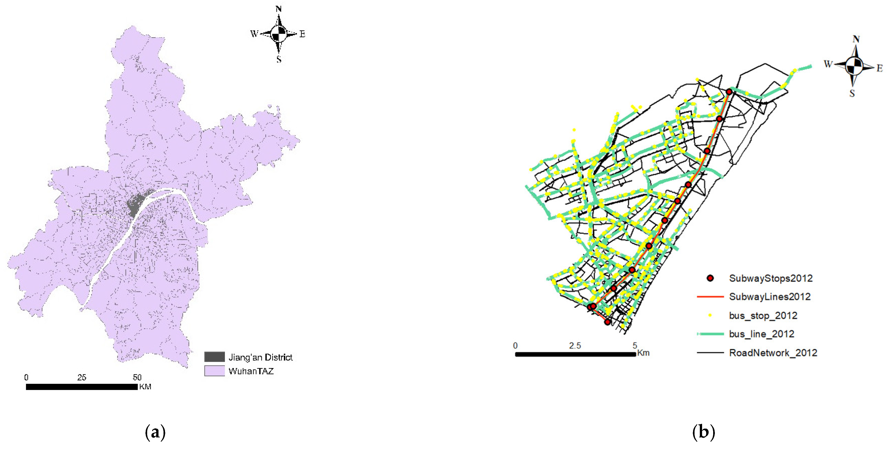
3.1. Data

This study considers the Jiang’an District, City of Wuhan, China as the case study. The City of Wuhan is located at a latitude of 29°58′–31°22′ north and a longitude of 113°41′–115°05′ east. The City of Wuhan has 13 districts under its jurisdiction. As of the end of 2019, the total area of Wuhan was 8569.15 ${\mathrm{km}}^2$, with a resident population of 11.212 million. In recent years, rail rapid-transit development in Wuhan has accelerated. The length of completed rail-transport lines expanded considerably from 2011 to 2015, from 28.68 km to 125.64 km [60]. In addition, only line 1 is within the study region; line 1, which was constructed in 2004 and then extended in 2010 and 2014, was the only elevated rail line. It follows a path parallel to the Yangtze and Han rivers [60]. The City of Wuhan has around 4.77 million employees, working in various sectors in 2012, and it had increased to 5.06 million by 2015.

The employment data were obtained from the Wuhan Transportation Development Strategy Institute (http://www.whtpi.com) (accessed on 20 May 2022). Furthermore, employment by industry type was used to develop the transport model. The total number of parcels considered for this study was 871. There were 141 and 196 bus lines in service in 2012 and 2015, respectively. In 2012, there was only one subway line with 26 subway stations; by 2015, this was increased to 28 subway stations which are shown in

Table 1. Type study data of Jiang’an district.

Years	Bus Lines	Subway Stations	Population (Persons)	Space Quantity (Square Meter)	Parcels (Nos)
2012	141	26	921,700	36,417,232	871
2015	196	28	954,300	38,613,407

. In order to estimate the average space prices, the building floor space was split into four categories: residential, commercial, mixed residential–commercial, and mixed commercial–residential. The residential–commercial mix indicates that the density of residential building types is higher than commercial, while the commercial–residential mix indicates that the density of commercial buildings is higher than residential.

Table 2. Total space quantity (${\mathrm{m}}^2$) and average space price (Yuan/m²).

Years/Type	2012		2015
	Total Space Quantity	Average Space Price	Total Space Quantity	Average Space Price
Commercial	1,804,696	1804	2,179,442	2413
Mix (Commercial–Residential)	1,888,940	1792	2,013,994	2315
Residential	13,559,658	3409	14,804,345	4319
Mix (Residential–Commercial)	19,163,936	3398	19,615,624	4269

illustrates the total space quantity and average space price type data of the Jiang’an district between 2012 and 2015. As indicated in Table 2, the space quantity and average space price increased between 2012 and 2015. In addition, it was observed that the total space quantity of mixed commercial–residential increased by around 125,054 square meters between 2012 and 2015. The average space price of mixed commercial–residential and mixed residential–commercial increased by 29.18% and 25.63% between 2012 to 2015, respectively.

Figure 1a illustrates the 13 Districts of the City of Wuhan and Figure 1b shows the road network, bus line, bus stations, subway line, and subway stations. Figure 1c illustrates the building data from the year 2012 by building type (i.e., residential, commercial, mixed residential–commercial, and mixed commercial–residential) of the Jiang’an District at the parcel level; however, Figure 1d depicts accessibility to residential activities in the year 2012. The range of index values of accessibility indicate: low accessibility (10.96~11.84), low–medium accessibility (11.85~13.54), medium accessibility (13.55~14.38), medium–high accessibility (14.39~14.66), and high accessibility (14.67~15.07). The MLU module was developed using building data, which contain building type and floor-space quantity by space type. Furthermore, the ArcGIS spatial intersection analysis tool was used to aggregate the building floor space to the parcel level. Usually, MLU is divided into three types: vertical mix, horizontal mix, and a combination of both. However, due to the limitation of the data, in this study, only a horizontal mix was considered. Additionally, the price of residential and commercial floor space was acquired for the years 2012 and 2015. To support this study, a multimodal transport model was developed using population and employment by type, to calculate accessibility at the parcel level. Furthermore, the multimodal transport model was calibrated to validate the model’s accuracy.

3.2. Data Processing

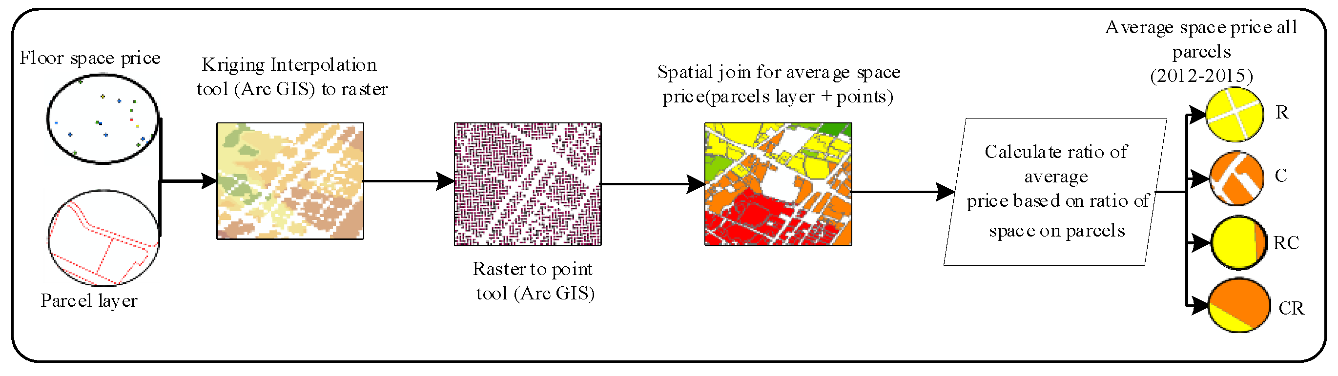
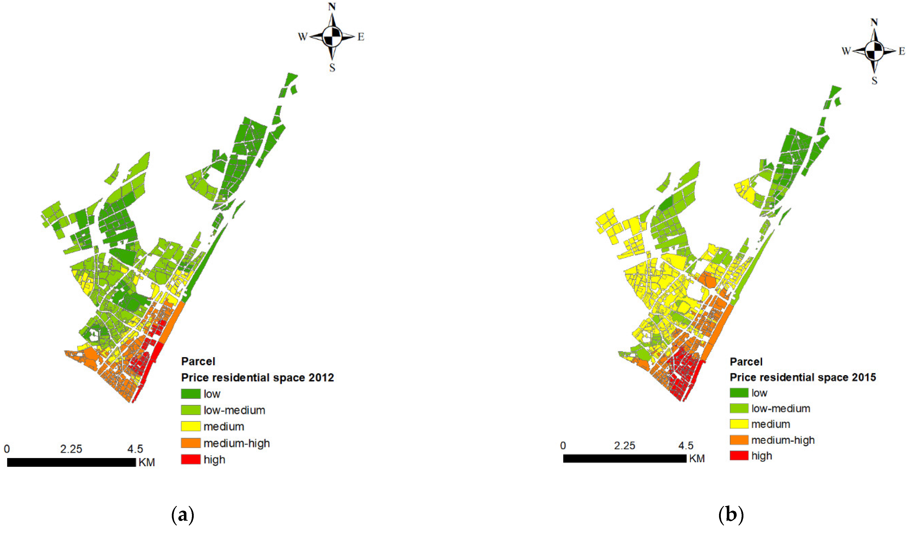
3.2.1. Price of Floor Space

Residential and commercial floor-space price data for the years 2012 and 2015 were obtained from the online real-estate website (https://fang.com/default.htm) (accessed on 20 May 2022). However, the floor-space price collected covers only part of the study area. This study used a kriging interpolation method to estimate the average floor-space price for the rest of the study area. By using this method, the raster data of floor-space price were obtained. After that, the “raster to point” tool was used in Arc Toolbox to convert the raster data of floor-space price into point data. Then, the point data of floor-space price and the parcels layer of the Jiangan district were spatially connected to estimate the average floor-space price for residential and commercial using “spatial join” tool, as shown in Figure 2. For the whole study area, we used the addresses of the locations to establish the latitude and longitude of residential and commercial buildings, matching them to real estate addresses using the website batchgeo (https://batchgeo.com) (accessed on 20 May 2022); then, the coordinates were converted to the standard WGS1984 coordinate system and visualized in the ArcGIS software, as shown in Figure 3. As mentioned earlier in Figure 1c, which contains residential, commercial, residential–commercial, and commercial–residential mixed land-use at the parcel level using density. However, buildings with low density are overlapped by other building types. Most of the study area has both residential and commercial land-use, as it is an urban area. While Figure 3 shows average floor-space prices for each floor-space type. It is observed from Figure 3c,d that most of the areas with high commercial buildings show high floor-space prices. In addition, space price (Yuan/m²) ranges are shown in Figure 3. In Figure 3a, the range of index values indicates space price: low space price (5683~6502), low–medium average space price (6503~7370), medium space price (7371~8520), medium–high space price (8521~10,070), and high space price (10,071~12,015). In Figure 3b, the range of index values indicates low space price (7673~8935), low–medium space price (8936~10,562), medium space price (10,563~12,472), medium–high space price (12,473~14,672), high space price (14,673~17,633). In Figure 3c the range of index values indicates low space price (12,928~14,883), low–medium space price (14,884~16,614), medium space price (16,615~18,988), medium–high space price (18,989~21,226), and high space price (21,227~22,518). Lastly, in Figure 3d, the range of index values indicates low space price (13,612~15,392), low–medium space price (15,393~17,879), medium space price (17,880~19,718), medium–high space price (19,719~23,292), and high space price (23,293~27,675).

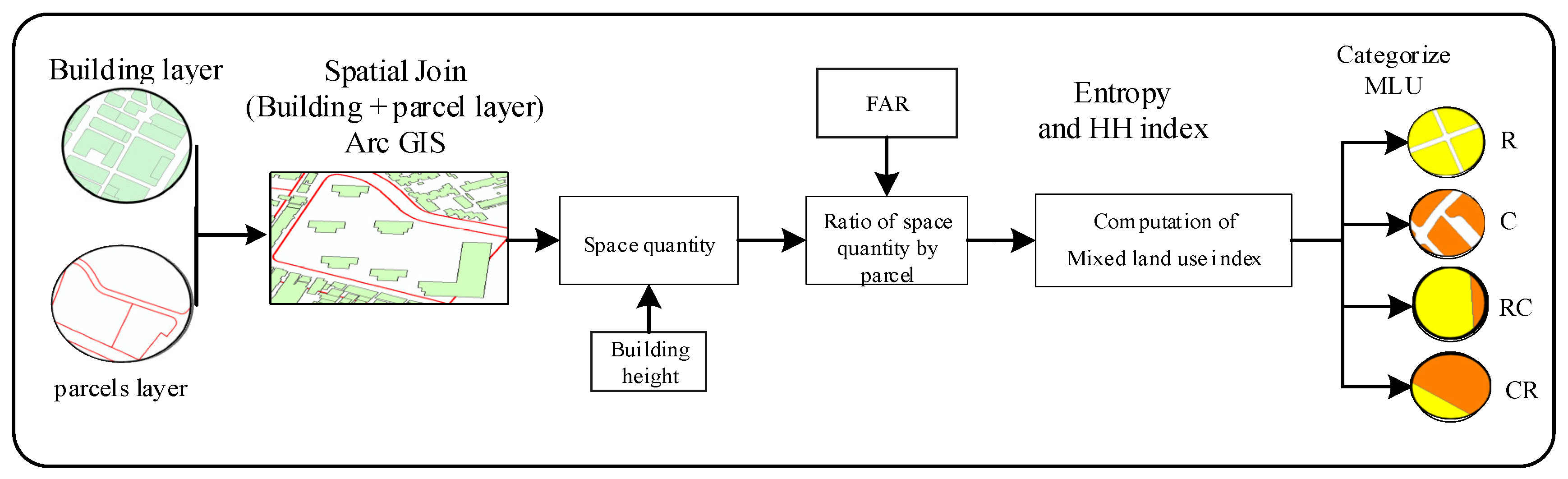
3.2.2. Preparation of Mixed Land-Use Data

MLU is an important tool of urban planning and spatial planning nowadays, since it introduces diverse land-uses into an area. For example, the mixed land-use strategy is regarded a key component for improving walkability in urban areas.

The building data for the years 2012 and 2015 were used to develop the model. The parcel data, which contain the building area, number of floors, and building use type, were extracted. The building uses for the years 2012 and 2015 were extracted using the data describing current land-use at the parcel level. Spatial analysis, using the intersection tools of ArcGIS, was used to extract the parcel data. Furthermore, the extracted parcel area and the number of floors in each building type were used to calculate the built space quantity by type of parcels. To determine the level of mixed land-use, the HHI and entropy indexes were used. From the output from these steps, the buildings were categorized into residential, commercial, mixed residential–commercial, and mixed commercial–residential with the mixed land-use degree, as shown in Figure 4.

The floor area ratio (FAR) is the ratio of the total floor area of the building to the size of the land on which it is constructed. It is frequently used to calculate the building-to-land ratio. It is one of the regulations in city planning to aggregate the building data and obtain the total construction area to determine the FAR of each parcel [14]. The mathematical form of FAR is shown in Equation (1).

$$\left(FAR\right)=\frac{{{\displaystyle \sum }}_{j=1}^n{B}_i\times F_i}{A}$$

(1)

—

$B_i$ represents the total floor area $\left({\mathrm{m}}^2\right)$ of the building $i$;

—

$F_i$ represents the number of floors of the $i$ the building; and

—

$A$ represents the area of the parcels under computation.

The maximum amount of developable space refers to the amount of space permitted by the land developer. This information is derived from developable land-use and the maximum floor area ratio. Data of each Parcel in the Jiang’an District for the years 2012 and 2015 is depicted in Equation (2).

$$Max{Q}_i^p=A{L}_i^p\times FA{R}^p$$

(2)

—

$Max{Q}_i^p$ represents the maximum developable space of the $p$ land-use type in the parcels i;

—

$A{L}_i^p$ represents the developable land of the $p$ land-use type in parcels i; and

—

$FA{R}^{p }$ indicates the maximum floor area ratio of the $p$ land-use type.

Two different mixed land-use indexes were used to analyze the data: entropy and HH indexes. The entropy index is a relative measure of an area’s land-use types, with a higher entropy degree indicating a higher mixed land-use [4]. The HH index is the inverse of the entropy index, with a higher degree indicating a lower mixed land-use. The entropy index is used to quantify the mixed land-use diversity. The degree of land-use diversity within a specific area is calculated by Equation (3) as follows:

$$Entropy=-{\displaystyle \sum }_{i=1}^k{P}^i\ln P^i$$

(3)

where

—

$P^i$, is the percentage of each land-use type $i$ in the area; and

—

$k$ is the total number of land-use types.

The HH index relates to mixed land-use status and is applied to the situation of market concentration in economics [30]. The HHI is calculated using Equation (4).

$$HHI={\displaystyle \sum }_{i=1}^k{(100\times P^i)}^2$$

(4)

—

$P^i$ is the percentage of land-use $i$ in the given area; and

—

k is the number of land-use types in parcels $i$.

Figure 5a,c show the entropy index for the years 2012 and 2015. A value of 0.057–0.69 and 0.58–0.69 from 2012 and 2015, respectively, indicates a high degree of mixed land-use patterns; a value of 0.21–0.38 and 0.22–0.39 indicates a medium degree of mixed land-use patterns; and a value of 0.010–0.20 and 0.010–0.21 indicates a low degree of mixed land-use patterns. The results from the entropy index depict that most parcels show a high level of mixed land-use patterns. Moreover, Figure 5b,d depict the HH index for the years 2012 and 2015. A value of 50–57 and 50–58 from 2012 and 2015, respectively, indicates a high level of mixed land-use, while a range of 84–99 indicates a low level of mixed land-use patterns. In addition, an entropy value of 0.0 and an HHI of 100 indicate that a parcel only contains one land-use pattern. As indicated by the HH index values in Figure 5b,d, most parcels have a high level of mixed land-use.

3.3. Methods

A deep neural network (DNN) is an ANN with multiple hidden layers between the input and output layers. DNNs can solve complex nonlinear relationships. ANN is a robust technique that receives a set of inputs, performs progressively complex calculations on them, and outputs results to solve real-world problems such as forecasting and classification. Thus, in this study, DNN, including MLP and LSTM, were used to analyze the effect of transportation supply on mixed land-use. The workflow is depicted in Figure 6. The primary steps are as follows:

(1)

The data for the models representing transportation supply (road network, bus stops and lines, subway lines and stops, and others), floor-space price (by type), and land-use data (construction area, developable land, floor area ratio, building, and other land-use data) were prepared;

(2)

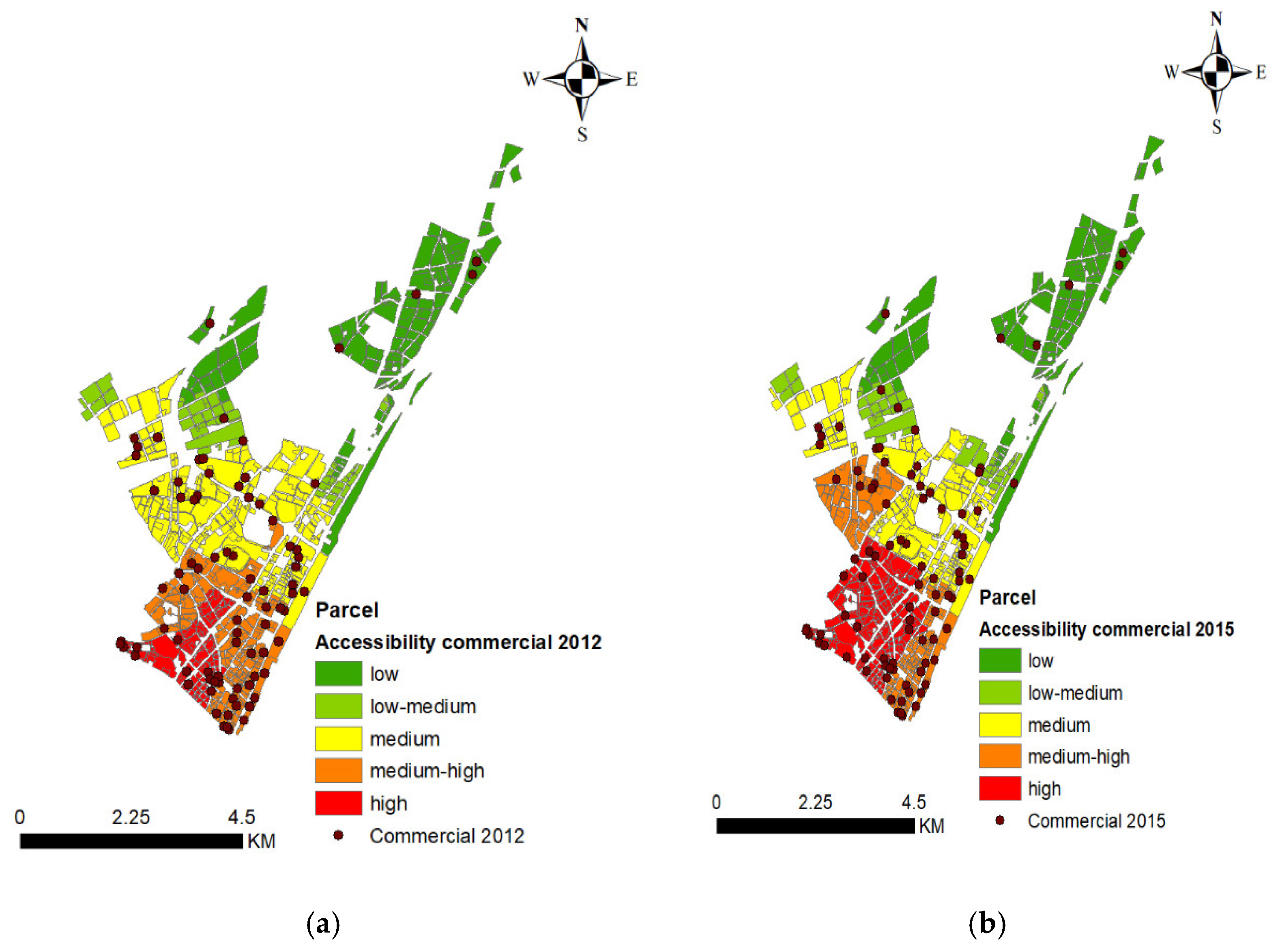
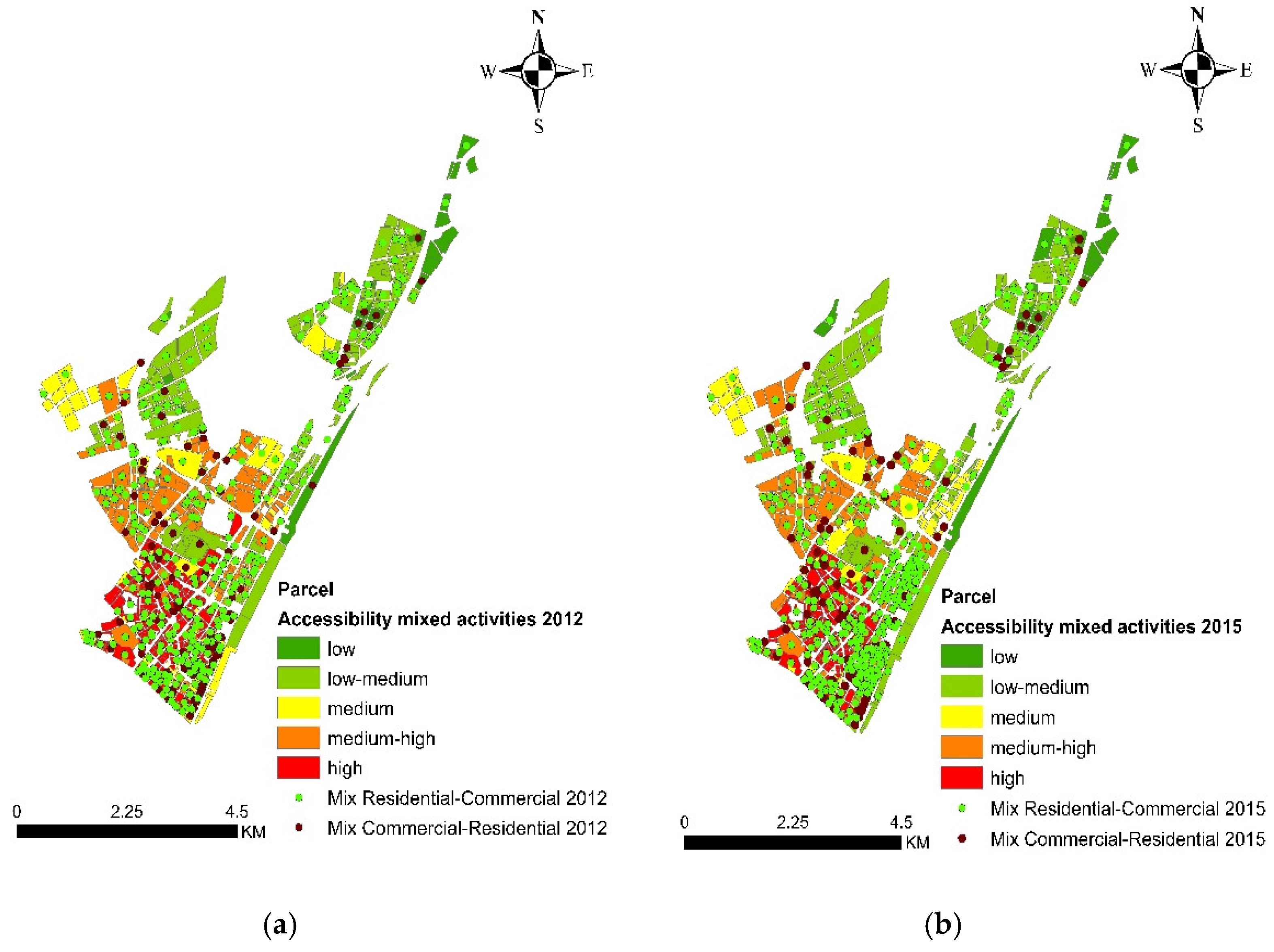
The developed multimodal transport model was used to calculate accessibility to residential, commercial, and mixed land-uses at the parcel level for the years 2012 and 2015;

(3)

Due to the data limitation, the average floor-space prices were estimated using the Kriging interpolation tool at the parcel level;

(4)

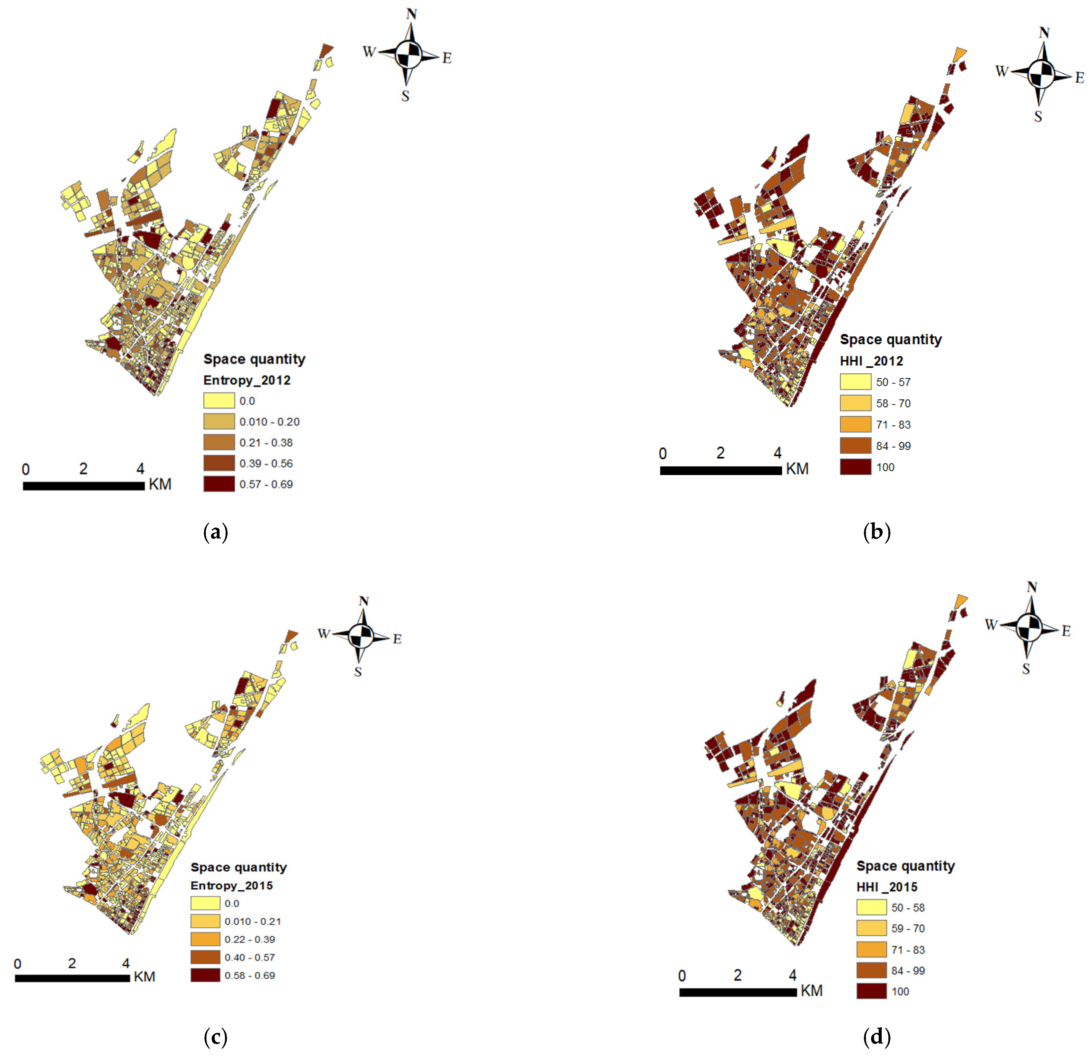
The mixed land-use data were prepared at the parcel level in ArcGIS using the “spatial join” and “intersection analysis” tools, and the Entropy and HH indexes were used to quantify the degree of mixed land-use;

(5)

Deep neural networks (MLP and LSTM) were used to forecast future years of mixed land-use types at the parcel level. Moreover, the change in space quantity due to transportation supply and floor-space price changes between 2012 and 2015 were analyzed;

(6)

Finally, the accuracy of the developed MLP and LSTM models were compared.

The model examined the effect of transportation supply on MLU patterns at the parcel level in the Jiang’an District using MLP and LSTM. The models developed for this study are presented as follows.

3.3.1. Transport Model

The transport model was developed and then used to calculate utility-based accessibility measures at the parcel level from 2012 to 2015. This model was developed using a multimodal network approach to represent the interactions between all transportation modes. As mentioned in the data Section 3.1, various datasets were adopted and several steps were taken, which enabled the calculation of accessibility measures for the residential, commercial, mixed residential–commercial, and mixed commercial–residential land-uses at the parcel level. These accessibility measures were used as the input to the MLP and LSTM models as independent variables. The model processes are as follows:

(1)

The trip generation module starts with the calculation of trip production and attraction by trip purpose;

(2)

The trip distribution module distributes these trips to each parcel using the gravity approach. Furthermore, mobile phone signal data are used to calculate and calibrate trip length frequency;

(3)

A mode choice module, which is based on an absolute nested logit structure, distributes trips to different modes based on the utility associated with each mode;

(4)

Trip assignment module: The trip assignment process reproduces the patterns of vehicular movements on the transportation system, which can be seen when the travel demand is satisfied. To obtain the volume of traffic on the network links and estimate aggregate network measures, the travel pattern of each O-D pair (origin to destination) is estimated. The assigned model generates congested skims which are fed back to the distribution model. The model uses the congested skim to perform the distribution and mode choice. This enables the production of utility-based accessibility based on congested time, which is input to MLP and LSTM models, as shown in Equation (5).

$$A_i= \mathrm{Ln}(1+{\displaystyle \sum }_{j=1}^n={\displaystyle \sum }_{k=1}^m{e}^{U_{ij}^k}\times O_J)$$

(5)

where

—

$A_i$ is the accessibility of parcel i;

—

i and j are both parcel numbers;

—

k is one of the modes of transportation;

—

n is the total number of parcels;

—

m is the total number of modes of transportation;

—

$U_{ij}^k$ is the utility generated by the transportation mode k from parcel i to parcel j; and

—

$O_j$ is the service or opportunity of parcel j;

—

$+1$ in case of no activity.

3.3.2. Multilayer Perceptron (MLP) Algorithms

Artificial intelligence-based algorithms (e.g., heuristics, metaheuristics) are promising and rapidly expanding application areas of urban planning and transportation, including online learning [61], vehicle routing [62], delayed start parallel evolutionary algorithm [63], non-dominated sorting genetic algorithm, multi-objective particle swarm optimization [64], and multi-objective optimization [65,66]. The multi-objective spatial optimization of land-use depends on two factors: land-use population capacity and land-use carbon emission [67]. In addition, DNNs are improved versions of traditional ANNs, with multiple layers. Due to their superior ability to learn nonlinear input–output mapping, DNN models have recently been gaining more popularity. However, recent research has demonstrated significant potential for ANN-based approaches in land-use changes [49,50]. The ANN approach was used to investigate the impact of transportation supply on mixed land-use changes at the parcel level. The ANN approach has four steps: (1) build the network, inputs, and outputs; (2) select a subset of the inputs and train neural networks; (3) validate ANN with the dataset of inputs; and (4) utilize ANN for a future year. One of the most common ANN architectures is the multi-layer perceptron (MLP) network, which is also employed in this study. MLP is a framework for feed-forward networks that provides non-linear functional mapping between a set of input and output variables. It has four layers: one input, two hidden, and one output. Neurons are represented by circles, while lines represent unidirectional interconnections between neurons in the corresponding layer [68]. The structure of MLP is shown in Figure 7.

To evaluate the effect of transportation supply on mixed land-use change, the input layer contains neurons corresponding to the input value of each neuron (features) $x_i$. The input layer considers 13 input values: space quantity 2012, average space price, maximum available space quantity, HH index, entropy index, different accessibility measures (residential, commercial, mixed residential–commercial), etc. The neurons in the output layer predict space quantity for 2015 for all parcels and the ratio of quantities of different types of land-uses by the HH index or entropy index. The weighted linear combination of the input variables is the output of the hidden neuron. In an MLP with one hidden layer, the sigmoid activation function is utilized to activate the mth hidden neuron.

Equations (6) and (7) show the mathematical formulation of the MLP. Each neuron has its regression model, which consists of input data, weights, thresholds, activation functions, and outputs.

$$Z_i={{\displaystyle \sum }}_{i=1}^m{w}_{ij}\times x_i+b_j$$

(6)

$$Output Y_i=\mathrm{F}\left(Z_i\right)=\{\begin{array}{c}1 if {\displaystyle \sum }_{i=1}^m{w}_{ij}\times x_i+b_j\ge 0\\ 0 if {\displaystyle \sum }_{i=1}^m{w}_{ij}\times x_i+b_j<0\end{array}$$

(7)

where

—

$Z_i$ is the output value of the neuron j;

—

$x_i$ is the input value of the neuron i (space quantity 2012, accessibility, price, etc.);

—

$w_{ij}$ is the weight between the neuron i and neuron j;

—

$b_j$ is the threshold (bias) of the neuron j;

—

$Y_i$ is the output value after activation of the neuron j (the predict of space quantity 2015); and

—

$\mathrm{F}$ is the activation function.

The weights are assigned to the input layers in the MLP once the input layers have been determined. These weights aid in determining the importance of any given variable, with larger weights contributing more to the final result than lower weights. Following that, all of the inputs are multiplied by their respective weights, then summed, and a threshold is established before they are fed through an activation function that has been defined. Thus, the output of that neuron becomes the input of the next neuron. Forward propagation is the term used to describe transmitting data from one layer to the next. All inputs are adjusted so that they fall within the range of (0, 1) [49].

The ultimate purpose of forwarding propagation of the MLP is to minimize the loss function. Thus, the network feeds the output data into the input and adjusts its weights and thresholds according to a loss function to attain a convergent point or local minimum, a process known as backpropagation. Gradient descent is used to optimize the model’s orientation in order to reduce loss or error. Throughout each training process, the network’s parameters gradually converge to a minimal value [69].

The selection of hyperparameters, such as activation functions, optimizers, etc., are critical in MLP. They show the ability, speed, and accuracy of the MLP training. The MLP hyperparameters include the learning rate, the batch size for training, the number of hidden layers, the number of hidden layer neurons, and the number of iterations.

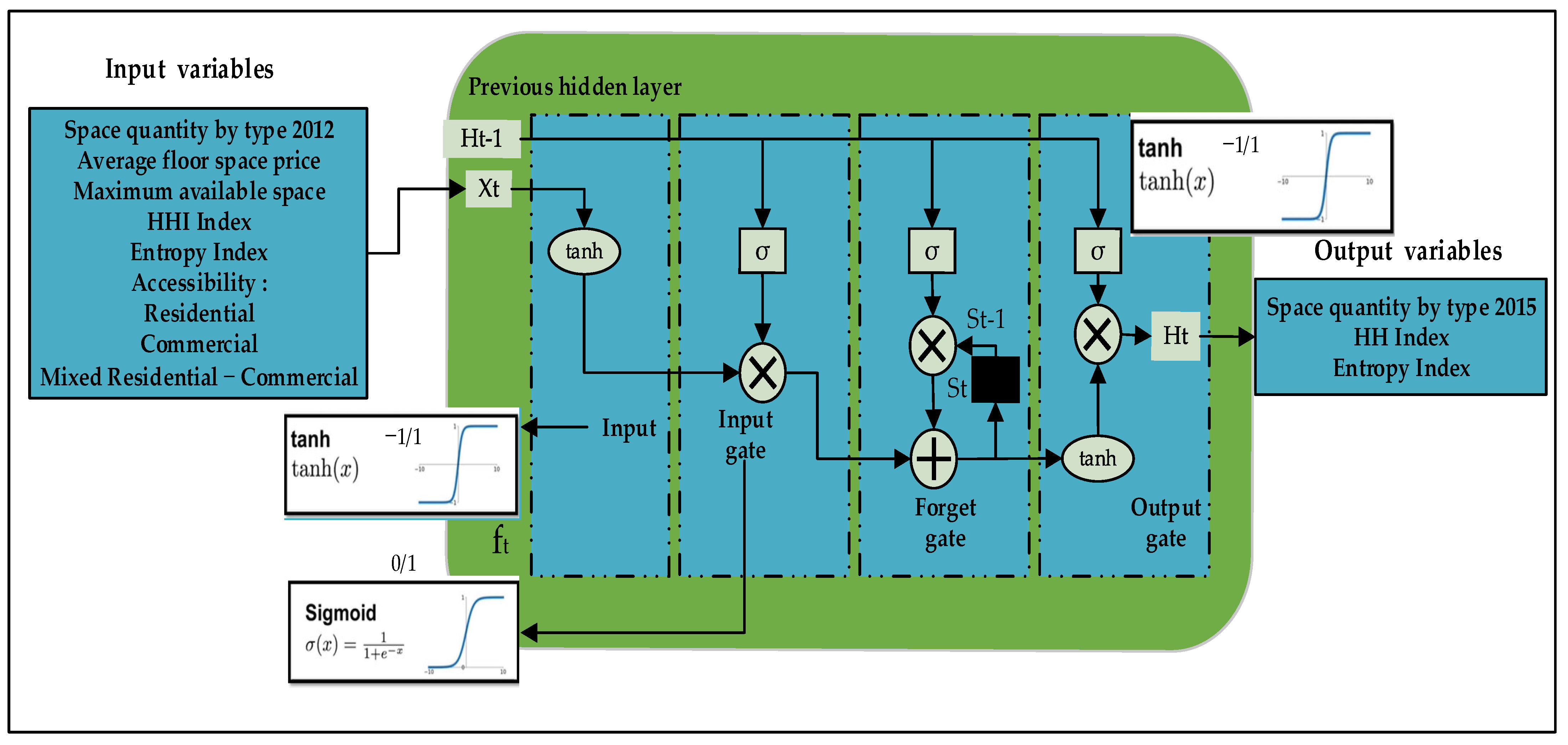
3.3.3. Long Short-Term Memory (LSTM) Algorithms

Recurrent neural networks (RNNs) are a subtype of neural networks designed to deal with sequential data types such as text and time series. However, due to the vanishing gradient problem, conventional RNNs cannot capture long-term dependencies in data [70]. To address this issue, the long short-term memory (LSTM) network, a subtype of RNN, was developed. Due to its larger memory capacity, LSTM is more frequently used than traditional RNN. The cell state, sigmoid activation, forget gate, input gate, output gate, and $tan h$ activation are all critical elements of LSTMs because they control the flow of relevant information through the network. The gates control the addition and removal of information from the cell state at each processing step [71]. Gates have sigmoid activation, which multiplies values between 0 and 1 to determine the percentage of data that will be retained or deleted. If the input equals 0, then the information is lost; if the input equals 1, the data are fully retained. $Tan h$ activation produces values in the range of −1 to 1. The process of RNNs is shown in Equations (8)–(13), and Figure 8 shows the LSTM cell neural network structure.

$$i_t=\sigma \left(w_i\left[h_{t-1}, x_t\right]+b_i\right)$$

(8)

$$f_t=\sigma (w_f\left[h_{t-1}, x_t\right]+b_f$$

(9)

$$o_t= \sigma \left(w_o\left[h_{t-1},{ x}_t\right]+{ b}_o\right)$$

(10)

$${ g}_t=tan h\left(w_g\left[h_{t-1},{ x}_t\right]+{ b}_g\right)$$

(11)

$$c{ }_t=f_t\times c_{t-1}+i_t\times g_t$$

(12)

$$h{ }_t=o_t\times tan h\left(c_t\right)$$

(13)

where

—

$c_t$ denotes cell state, and $h_t$ denotes the output for training 70% of space quantity 2015 and predicting 30% of space quantity 2015, at time step t;

—

$f_t$ denotes forget state, $o_t$ represents the output gate, and $\mathsf{\sigma }$ represents the sigmoid function;

—

$w$ represents the weight, $b$ represents bias, and $g_t$ denotes a vector of the new candidate value called cell activation;

—

$f_{t }$ represents a value between 0 and 1, which means the ratio of old information that will be passed to the new cell state; and

—

$i_t$ decides the ratio of each value in a sequence from $g_t$ that will be preserved.

From the training and prediction of floor-space quantity 2015, the LSTM model was used in a case study of the Jiang’an District in Wuhan, China, with model inputs encoded as transportation supply, average space price, and floor-space quantity. A total of 70% of the datasets were used for training purposes and the remaining 30% were used for testing the models.

Figure 8. LSTM cell neural network structure.

Figure 8. LSTM cell neural network structure.

4. Results and Discussion

Deep neural network models, namely MLP and LSTM techniques, were used to analyze the effects of transportation supply on MLU at the parcel level by taking a case study of the Jiang’an District, Wuhan, China. The dataset from the Jiang’an District contains 871 parcels for 2012 and 2015.

4.1. Accessibility and MLU Change at the Parcel Level (2012 and 2015)

Since accessibility to employment activities is positively correlated with the level of service (LOS) of the transportation system and the employment location, this paper applied three categories of employment accessibility measures, including those to residential, commercial, and mixed residential–commercial areas in the Jiang’an District, Wuhan for the years 2012 to 2015, as shown in Figure 9 and Figure 10.

In this study, correlation analyses were carried out to check the correlation between land-use and transportation indicators.

Table 3. Correlation matrix.

	Pearson Correlation	[1]	[2]	[3]	[4]	[5]	[6]	[7]	[8]	[9]	[10]	[11]	[12]	[13]
[1]	Mixed Accessibility (RCA)	1	0.789 **	0.798 **	−0.144 **	−0.043	−0.172 **	−0.140 **	0.050	0.097 **	−0.178 **	−0.143 **	0.047	0.096 **
[2]	Commercial Accessibility (CA)	0.789 **	1	0.988 **	0.373 **	0.453 **	0.060	0.078 *	−0.124 **	−0.019	0.055	0.083 *	−0.133 **	−0.022
[3]	Residential Accessibility (RA)	0.798 **	0.988 **	1	0.366 **	0.445 **	0.062	0.079 *	−0.103 **	−0.008	0.057	0.084 *	−0.114 **	−0.014
[4]	Mixed-Space Price 2012 (RCP)	−0.144 **	0.373 **	0.366 **	1	0.924 **	0.356 **	0.377 **	−0.216 **	−0.154 **	0.310 **	0.361 **	−0.202 **	−0.160 **
[5]	Mixed-Space Price 2015 (RCP)	−0.043	0.453 **	0.445 **	0.924 **	1	0.341 **	0.333 **	−0.195 **	−0.143 **	0.333 **	0.348 **	−0.201 **	−0.147 **
[6]	Commercial Space (CS) 2012	−0.172 **	0.060	0.062	0.356 **	0.341 **	1	−0.050	−0.063	−0.074 *	0.835 **	−0.042	−0.063	−0.075 *
[7]	Commercial–Residential Space (CRS) 2012	−0.140 **	0.078 *	0.079 *	0.377 **	0.333 **	−0.050	1	−0.082 *	−0.096 **	−0.042	0.924 **	−0.082 *	−0.090 **
[8]	Residential Space (RS) 2012	0.050	−0.124 **	−0.103 **	−0.216 **	−0.195 **	−0.063	−0.082 *	1	−0.122 **	−0.063	−0.084 *	0.914 **	−0.103 **
[9]	Residential–Commercial Space (RCS) 2012	0.097 **	−0.019	−0.008	−0.154 **	−0.143 **	−0.074 *	−0.096 **	−0.122 **	1	−0.074 *	−0.092 **	−0.107 **	0.965 **
[10]	Commercial Space (C S) 2015	−0.178 **	0.055	0.057	0.310 **	0.333 **	0.835 **	−0.042	−0.063	−0.074 *	1	−0.051	−0.063	−0.075 *
[11]	Commercial–Residential Space (CRS) 2015	−0.143 **	0.083 *	0.084 *	0.361 **	0.348 **	−0.042	0.924 **	−0.084 *	−0.092 **	−0.051	1	−0.084 *	−0.100 **
[12]	Residential Space (RS) 2015	0.047	−0.133 **	−0.114 **	−0.202 **	−0.201 **	−0.063	−0.082 *	0.914 **	−0.107 **	−0.063	−0.084 *	1	−0.124 **
[13]	Residential–Commercial Space (RCS) 2015	0.096 **	−0.022	−0.014	−0.160 **	−0.147 **	−0.075 *	−0.090 **	−0.103 **	0.965 **	−0.075 *	−0.100 **	−0.124 **	1

Note: * = correlation is significant at the 0.05 level (2-tailed), ** = Correlation is significant at the 0.01 level (2-tailed); R = residential, C = commercial, RC = residential–commercial, CR = commercial–residential.

shows the degrees of correlation among variables. Using the dependent variable of space quantity for the following land-use types (R = residential, C = commercial, RC = residential–commercial, CR = commercial–residential) in the Year 2015 as an example, it is found that most of the variables are highly correlated with the quantity (see those numbers highlighted with * or **). The results showed that residential accessibility is highly correlated with residential space, and commercial accessibility has a high correlation with commercial space. Moreover, the mixed accessibility encouraged mixed land-use development in that places with high mixed accessibility have a high level of mixed land-use patterns, as shown in Table 3. In addition, the results depict that high accessibility encourages a high level of mixed space for residential/commercial uses, as shown in Table 3. Likewise, areas with high accessibility are found to have high space prices, which indicates that accessibility influences space prices significantly.

Figure 9a,b illustrate the accessibility to residential activities and residential spaces developed between 2012 and 2015. The results indicate that parcels with high accessibility to residential activities have high-density residential space developed. In 2015, it was found that the residential space was significantly developed in parcels with high accessibility. These results indicate that there is a strong relationship between accessibility and developed space. In addition, Figure 9a,b indicate the range of index values of accessibility for residentials in 2012 and 2015: low accessibility (10.96~11.84), low–medium accessibility (11.85~13.54), medium accessibility (13.55~14.38), medium–high accessibility (14.39~14.66), and high accessibility (14.67~15.07).

Figure 10a,b depict the accessibility to commercial activities from 2012 to 2015 and the developed space quantity. The results indicate that most of the areas with high accessibility to commercial activities showed a high density of developed commercial space quantity. With the increase in accessibility to commercial activities in 2015, especially in the middle of the Jiang’an District, an area along subway line 1, a significant increase in commercial space quantity was found. These key results indicate that there is a strong relationship between accessibility and space quantity. Figure 10a,b indicate the range of index values of accessibility for commercial space in 2012 and 2015: low accessibility (8.774~11.55), low–medium accessibility (11.56~12.97), medium accessibility (12.98~13.80), medium–high accessibility (13.81~14.47), and high accessibility (14.48~15.01).

Figure 11a,b depict the accessibility to mixed (RC and CR) activities from 2012 to 2015 and the developed mixed-space quantity. The results indicate that most of the areas with high accessibility to mixed activities showed a high density of developed mixed (RC and CR)-space quantity. With the increase in accessibility to mixed activities in 2015, such as in the south and center of the Jiang’an District, close to the city center and subway line 1, a significant increase in mixed-space quantity was found. These key results indicate that there is a strong relationship between mixed accessibility and mixed-space quantity. Figure 11a,b indicate the range of index values of accessibility for mixed residential–commercial in 2012 and 2015: low accessibility (7.863~10.54), low–medium accessibility (10.55~11.70), medium accessibility (11.71~12.84), medium–high accessibility (12.85~13.36), and high accessibility (13.37~13.64).

Table 4. The total number of the buildings changed from 2012 to 2015 by parcel type in the Jiang’an district.

The Total Number of the Building Changed by Parcel Type
2012/2015	C	CR	D	R	RC	Total Change
C	14	2	0	0	4	20
CR	4	54	10	0	11	79
N	13	4	0	97	6	120
R	3	6	392	680	54	1132
RC	0	317	379	75	705	1476
Total Change	31	383	781	852	780	2827

Note: R = residential, C = commercial, RC = mix (residential–commercial), CR = mix (commercial–residential), D = demolished, N = new development.

illustrates the number of buildings that changed from 2012 to 2015. As indicated in Table 4, the mixed RC shows the highest incidence of change to mixed CR from 2012 to 2015. Meanwhile, the incidence of mixed CR change to RC was found to be relatively low compared to other mixed changes. In addition, it was observed that 75 buildings changed from RC to residential. However, it was observed that 54 buildings changed from residential to RC and 392 buildings were demolished. Moreover, it was observed that only 4 buildings changed from commercial to RC, and 2 buildings changed to CR. The total number of buildings changed was recorded at around 2827.

Table 5. Total space quantity change from 2012 to 2015 in Jiang’an district by Parcel type.

Total Space Quantity Change (m2)
2012/2015	C	CR	D	R	RC	Total Change
C	73,890	2006	0	0	2856	78,751
CR	1223	62,629	14,231	0	25,604	103,686
N	249,380	47,042	0	769,870	2431	1,068,723
R	45,352	53,058	135,051	848,800	247,270	1,329,531
RC	0	63,122	91,569	40,496	903,525	1,098,713
Total Change	369,844	227,857	240,851	1,659,167	1,181,686	3,679,405

Note: R = residential, C = commercial, RC= mix (residential–commercial), CR = mix (commercial–residential), D = demolished, N = new development.

illustrates how space quantities changed at the parcel level from 2012 to 2015. For instance, in mixed residential–commercial spaces in 2012, no space quantity changed to commercial in 2015, and a 63,122 square-meter space changed to mixed commercial–residential. Similarly, a 91,569 square-meter space was demolished during the period from 2012 to 2015, a 40,496 square-meter space changed to residential, and a 903,525 square-meter space remained unchanged. Moreover, for mixed commercial–residential in 2012, no space quantity changes to residential 2015 were recorded, and a 25,604 square-meter space changed to mixed residential–commercial. Similarly, a space of 14,231 square meters was demolished during the period of 2012 to 2015, a space of 1223 square meters changed to commercial, and a space of 62,629 square meters remained unchanged. The total change in space quantity was recorded as 3,679,405 square meters.

Figure 12 illustrates that most mixed residential–commercial and mixed commercial–residential spaces increased by 451,688 square meters and 125,054 square meters from 2012 to 2015, respectively. From 2012 to 2015, these areas had high accessibility, especially in the middle of the Jiang’an District, an area along subway line 1. However, mixed residential and commercial have increased relatively by 1,244,687 square meters and 374,746 square meters in the study area, respectively. Moreover, accessibility to commercial land increased in 2015. This means that increased accessibility due to public transportation (e.g., subway or regular bus) promotes mixed residential–commercial and residential development, but has little effect on mixed commercial–residential and commercial space development. A preferred commercial location may be close to major roads, allowing for easier access to the goods used in commercial and mixed commercial–residential parcels to meet the demand of customers.

4.2. Parameter Settings and Model Training

There is a strong association between mixed land-use, accessibility, and space price. As mentioned earlier in Section 2.2, several factors, such as space prices and accessibility, influence mixed land-use density, the results show that high-accessibility areas tend to have high mixed-land and space prices, whereas low-accessibility areas have low mixed-land-use density and space prices [6,14,44,45]. Due to building, accessibility, and average space quantity data, DNNs can capture complex nonlinear relationships [48]. This paper uses deep neural networks (MLP, LSTM) to analyze the relationship between the mixed land-use pattern, which is the dependent variable, and accessibility and floor-space price as independent variables, with 871 parcels in the case study, utilizing Keras with Tensor Flow as the framework for building the network in Python. The input variables were used for training and testing the LSTM and MLP models. The input nodes and outputs of the parcel-level mixed land-use prediction model based on deep neural network nodes are shown in

Table 6. Input and output data to the deep neural network model.

Input Variables for Training (70% of Data Samples)	Output Variables for Training	Input Variables for Testing (30% of Data Samples)	Output Variables for Testing
Average floor-space price from 2012 to 2015	Space quantity at parcel level 2015:	Average floor-space price from 2012 to 2015	Space quantity at parcel level 2015:
Maximum available space quantity	Residential	Maximum available space quantity	Residential
Space quantity at parcel level 2012	Commercial	Space quantity at parcel level 2012	Commercial
Accessibility from 2012 to 2015 by: residential, commercial, mixed residential–commercial	Residential–commercial	Accessibility from 2012 to 2015 by: residential, commercial, mixed residential–commercial	Residential–commercial
	Commercial–residential		Commercial–residential

.

The MLP model comprises one input layer, two hidden layers for balancing simulation accuracy and speed, and a final output layer. The MLP and LSTM models were trained for 3000 epochs. The LSTM model consists of one input layer, two layers with a size of 100 each, two completely connected layers, and a final output layer. The remaining parameters are as follows: batch size: 16, learning rate: 0.001, input variables: 13, and hidden layer neurons: 128. ADAM optimization was used to enhance the prediction accuracy for the MLP and LSTM models comprised assessing missing data, imputing missing values, and investigating outliers and duplicated records.

4.3. Comparison of Forecasting Accuracy of MLP and LSTM Models

Table 7. Comparison of the forecasting errors of MLP and LSTM (training).

Models	MLP Training Errors								LSTM Training Errors
Error\Land Type	Single-Use Errors (%)		Mixed CR Errors (%)			Mixed RC Error (%)			Single-Use Errors (%)		Mixed CR Errors (%)			Mixed RC Error (%)
	C	R	C	R	CR	C	R	RC	C	R	C	R	CR	C	R	RC
90th Percentile	10.36	7.02	3.31	2.37	5.68	2.13	3.32	5.45	3.78	3.68	1.38	1.15	2.53	1.08	1.60	2.68
80th Percentile	2.22	1.66	1.06	0.76	1.82	0.79	1.24	2.03	2.35	1.40	1.05	0.87	1.92	0.78	1.16	1.94
70th Percentile	0.75	0.99	0.74	0.53	1.27	0.52	0.81	1.33	0.70	0.96	0.71	0.51	1.22	0.57	0.74	1.31
50th Percentile	0.19	0.53	0.29	0.21	0.50	0.18	0.28	0.46	0.11	0.27	0.36	0.18	0.54	0.13	0.29	0.42
Average error	2.41	1.99	1.05	0.75	1.80	0.71	1.11	1.82	1.40	1.62	0.67	0.56	1.22	0.48	0.72	1.20

Note: R = residential, C = commercial, RC= mix (residential–commercial), CR = mix (commercial–residential).

shows the performance of the LSTM and MLP models during the training process. The models consider an effect between transportation supply and MLU at the parcel level during the training and forecasting process. The MLP model results in an average error of 1.80–1.82% for mixed use, and most of the 90th percentile errors are found to be lower than 5.68%; meanwhile, the LSTM model shows an average error of 1.20–1.22% for mixed use, and most of the 90th percentile errors were found to be lower than 2.68%. The MLP model results in an average error of 1.99–2.41% for single use, and most of the 90th percentile errors are found to be lower than 10.36%. Meanwhile, the LSTM model shows an average error of 1.40–1.62% for mixed use, and most of the 90th percentile errors are found to be lower than 3.78%.

Table 8. Comparison of forecasting errors of MLP and LSTM (testing).

Models	MLP Testing Errors								LSTM Testing Errors
Error\Land Type	Single Use Errors (%)		Mixed CR Errors (%)			Mixed RC Error (%)			Single Use Errors (%)		Mixed CR Errors (%)			Mixed RC Error (%)
	C	R	C	R	CR	C	R	RC	C	R	C	R	CR	C	R	RC
90th Percentile	20.17	10.00	8.45	5.28	13.73	6.54	4.77	11.31	16.58	9.43	6.16	4.30	10.46	4.03	5.14	9.17
80th Percentile	18.32	8.46	7.42	4.63	12.05	5.11	3.73	8.84	14.41	7.06	5.15	3.60	8.75	2.98	3.81	6.79
70th Percentile	16.44	6.79	5.85	3.65	9.51	4.33	3.16	7.49	12.25	5.31	3.85	2.69	6.54	2.30	2.94	5.24
50th Percentile	13.77	4.37	4.51	2.81	7.32	3.30	2.40	5.70	4.99	3.45	1.91	1.34	3.25	1.29	1.64	2.93
Average error	11.03	6.59	4.53	2.83	7.36	3.21	2.34	5.55	7.07	4.15	2.52	1.76	4.28	1.59	2.03	3.62

Note: R = residential, C = commercial, RC= mix (residential–commercial), CR = mix (commercial–residential).

presents the comparison results between the MLP and LSTM models. The MLP mixed CR model results in an average error of 7.36%, and the 90th percentile errors are found to be lower than 13.73%. Meanwhile, C in the MLP mixed CR model results in an average error of 4.53%, and the 90th percentile errors are found to be lower than 8.45%, while R in the MLP mixed CR model results in an average error of 2.83%, and the 90th percentile errors are found to be lower than 5.28%. The MLP mixed RC model results in an average error of 5.55% and the 90th percentile errors are found to be lower than 11.31%. Meanwhile, C in the MLP mixed RC model results in an average error of 3.21%, and the 90th percentile errors are found to be lower than 6.54%, while R in the MLP mixed RC model results in an average error of 2.34%, and the 90th percentile errors are found to be lower than 4.77%. The LSTM mixed CR model results in an average error of 4.28% and the 90th percentile errors are found to be lower than 10.46%. Meanwhile, C in the MLP mixed CR model results in an average error of 2.52%, and the 90th percentile errors are found to be lower than 6.16%, while R in the LSTM mixed CR model results in an average error of 1.76%, and the 90th percentile errors are found to be lower than 4.30%. The LSTM mixed RC model results in an average error of 3.62% and the 90th percentile errors are found to be lower than 9.17%. Meanwhile, C in the LSTM mixed RC model results in an average error of 1.59%, and 90th percentile errors are found to be lower than 4.03%, while R in the LSTM mixed RC model results in an average error of 2.03%, and the 90th percentile errors are found to be lower than 5.14%. These results indicate that the relationship between transportation supply and MLU is significant and, considering the accessibility factor, can also help to promote the accuracy of model predictions. The LSTM model has a lower error, indicating that it has a better capability for forecasting the dependency relationship between transportation supply and mixed land-use pattern than the MLP model.

Figure 13a shows the observed floor space and Figure 13b depicts the MLP-estimated floor space, while Figure 13c shows the MLP prediction errors. The value for the range of prediction errors indicates: low prediction errors (0.000~5.448), medium prediction errors (5.449~23.48), and high prediction errors (23.49~46.80). The findings reveal that the majority of parcels have low prediction errors across all space types (residential, commercial, and mixed-space types), whereas those showing a high error are usually large parcels with a low space quantity. Figure 14a depicts the observed floor space and Figure 14b shows the LSTM-estimated floor space, while Figure 14c shows the LSTM prediction errors. The value for the range of prediction errors indicates: low prediction errors (0.000~2.513), medium prediction errors (2.514~7.211), and high prediction errors (7.212~17.34). The results indicate that most of the parcels show low prediction errors for all space types (residential, commercial, and mixed-space types). The difference between the actual building type in 2015 with the MLP model prediction and the LSTM model prediction indicate that the LSTM model is more accurate at forecasting than MLP.

5. Conclusions

The objective of this study was to investigate the effects of transportation supply on mixed land-use. The study used deep neural network approaches such as LSTM and MLP models to evaluate the effect of transportation supply on mixed land-use at the parcel level. The study used 871 parcels of four MLU types in 2012 and 2015 in the Jiang’an District, Wuhan, China, as a case study.

According to the findings of this study, parcels with a high mixed accessibility usually have a high level of mixed land-use patterns, where the MLP and LSTM models result in an average error of 5.55–7.36% and 3.62–4.28%, respectively. Meanwhile, most of their 90^th percentile errors were less than 13.73% and 10.46% for the all-mixed land-use, respectively. These results indicated that the LSTM model performed better than the MLP model for all single and mixed land-use.

The study results showed that most parcels with mixed residential–commercial and residential land-use patterns changed significantly from the year 2012 to 2015 in areas that have high accessibility, such as in the south and center of the Jiang’an District, close to the city center and subway line 1. However, the mixed commercial–residential and commercial spaces remained relatively unchanged. Moreover, accessibility to commercial activities increased significantly in 2015 compared to 2012. This means that increased accessibility to public transit promotes mixed residential–commercial and residential land development, but has little effect on mixed commercial–residential and commercial land development. The MLP and LSTM models revealed that MLU is very sensitive to the supply of public transportation.

The proposed methods will allow accurate forecasting of a land-use pattern at the parcel level, even for parcels with few observations of a certain type, enabling policy analysis and simulations of development patterns across the city. Forecasting and corresponding simulations can assist decision-makers in better understanding various trade-offs that urban agents make when determining whether or not to take certain actions (e.g., whether to develop or not, what type of space, and how much to develop) within an urban real estate market. This study provides guidance and directions for a better understanding of the implications of transportation supply (especially that from public transportation) on MLU patterns. This paper studied the utility of the MLP and LSTM models in forecasting land-use patterns and using accessibility and average space-pricing as inputs. The models are found to produce accurate forecasts compared to those presented in the literature, and it is believed that they would be useful for simulating urban land-use patterns and for relevant policy analyses. The study has a few limitations that must be acknowledged:

• The mixed land-use data for a series of years are not available for comparison, so a study of land-use changes versus those of transportation supply cannot be carried out. More data are required to develop a pricing model of mixed-space patterns and also to investigate how density, mixed land-use, and accessibility affect prices, since this study only focused on accessibility.
• Future studies should consider additional data over a longer period in order to carry out the studies related to a “horizontal”, neighborhood-wide mixed-space pattern versus a “vertical”, within-building mixed-space use pattern.
• Due to the differences in state planning policies between underdeveloped and developed countries. A cross-national study is needed to obtain meaningful results.
• Based on the findings of this study, more advanced machine learning, ensembled approaches, and agent-based models, may be employed to improve the accuracy of forecasting different factors related to mixed land-use.

References

1. Shi, H.; Zhao, M.; Simth, D.A.; Chi, B. Behind the Land Use Mix: Measuring the Functional Compatibility in Urban and Sub-Urban Areas of China. Land 2021, 11, 2. [Google Scholar] [CrossRef]
2. Motieyan, H.; Azmoodeh, M. Mixed-use distribution index: A novel bilevel measure to address urban land-use mix pattern (A case study in Tehran, Iran). Land Use Policy 2021, 109, 105724. [Google Scholar] [CrossRef]
3. Carpio-Pinedo, J.; Benito-Moreno, M.; Lamíquiz-Daudén, P.J. Beyond land use mix, walkable trips. An approach based on parcel-level land use data and network analysis. J. Maps 2021, 17, 23–30. [Google Scholar] [CrossRef]
4. Yang, H.B.; Fu, M.C.; Wang, L.; Tang, F. Mixed Land Use Evaluation and Its Impact on Housing Prices in Beijing Based on Multi-Source Big Data. Land 2021, 10, 1103. [Google Scholar] [CrossRef]
5. Ghosh, P. Mixed Land Use Practices and Implications. Int. J. Sci. Dev. Res. (IJSDR) 2017, 2, 1–8. [Google Scholar]
6. Koster, H.R.A.; Rouwendal, J. The Impact of Mixed Land Use on Residential Property Values. J. Reg. Sci. 2012, 52, 733–761. [Google Scholar] [CrossRef] [Green Version]
7. Ali Aden, W.; Zheng, J.; Ullah, I.; Safdar, M. Public Preferences Towards Car Sharing Service: The Case of Djibouti. Front. Environ. Sci. 2022, 10, 889453. [Google Scholar] [CrossRef]
8. Safdar, M.; Jamal, A.; Al-Ahmadi, H.M.; Rahman, M.T.; Almoshaogeh, M. Analysis of the Influential Factors towards Adoption of Car-Sharing: A Case Study of a Megacity in a Developing Country. Sustainability 2022, 14, 2778. [Google Scholar] [CrossRef]
9. Wang, Z.; Safdar, M.; Zhong, S.; Liu, J.; Xiao, F. Public Preferences of Shared Autonomous Vehicles in Developing Countries: A Cross-National Study of Pakistan and China. J. Adv. Transp. 2021, 2021, 5141798. [Google Scholar] [CrossRef]
10. Raman, R.; Roy, U.K. Taxonomy of urban mixed land use planning. Land Use Policy 2019, 88, 104102. [Google Scholar] [CrossRef]
11. Hou, B.W.; Cao, Y.; Lv, D.Y.; Zhao, S.Z. Transit-Based Evacuation for Urban Rail Transit Line Emergency. Sustainability 2020, 12, 3919. [Google Scholar] [CrossRef]
12. Hellervik, A.; Nilsson, L.; Andersson, C. Preferential centrality—A new measure unifying urban activity, attraction and accessibility. Environ. Plan. B-Urban Anal. City Sci. 2019, 46, 1331–1346. [Google Scholar] [CrossRef]
13. Van Nes, A.; Berghauser Pont, M.; Mashhoodi, B. Combination of Space syntax with spacematrix and the mixed use index: The Rotterdam South test case. In Proceedings of the 8th International Space Syntax Symposium, Santiago, Chile, 3–6 January 2012. [Google Scholar]
14. Jayasinghe, A.; Madusanka, N.B.S.; Abenayake, C.; Mahanama, P.K.S. A Modeling Framework: To Analyze the Relationship between Accessibility, Land Use and Densities in Urban Areas. Sustainability 2021, 13, 467. [Google Scholar] [CrossRef]
15. United States Federal Highway Administration (FHWA). Program Value Cap Transit Oriented Development. 2018. Available online: https://www.fhwa.dot.gov/ipd/pdfs/fact_sheets/program_value_cap_transit_oriented_development.pdf (accessed on 20 May 2022).
16. Rad, T.G.; Alimohammadi, A. Modeling relationships between the network distance and travel time dynamics for assessing equity of accessibility to urban parks. Geo-Spat. Inf. Sci. 2021, 24, 509–526. [Google Scholar] [CrossRef]
17. Sungwon, L.; Bumsoo, L. Comparing the impacts of local land use and urban spatial structure on household VMT and GHG emissions. J. Transp. Geogr. 2020, 84, 102694. [Google Scholar] [CrossRef]
18. Huang, S.-W.; Hsieh, H.-I. The study of the relationship between accessibility and mixed land use in Tainan, Taiwan. Int. J. Environ. Sci. Dev. 2014, 5, 352. [Google Scholar] [CrossRef] [Green Version]
19. Xie, B.; Jiang, H.; Wang, L. Interactive planning research between urban transport and land use from the perspective of mixed-land use. In ICTE 2013: Safety, Speediness, Intelligence, Low-Carbon, Innovation; American Society of Civil Engineers: Reston, VA, USA, 2013; pp. 2882–2887. [Google Scholar] [CrossRef]
20. Ahmadzai, F. Analyses and modeling of urban land use and road network interactions using spatial-based disaggregate accessibility to land use. J. Urban Manag. 2020, 9, 298–315. [Google Scholar] [CrossRef]
21. Kim, D.; Jin, J. The Effect of Land Use on Housing Price and Rent: Empirical Evidence of Job Accessibility and Mixed Land Use. Sustainability 2019, 11, 938. [Google Scholar] [CrossRef] [Green Version]
22. Jin, J.; Paulsen, K. Does accessibility matter? Understanding the effect of job accessibility on labour market outcomes. Urban Stud. 2017, 55, 91–115. [Google Scholar] [CrossRef] [Green Version]
23. Frank, L.D. Land Use and Transportation Interaction. J. Plan. Educ. Res. 2016, 20, 6–22. [Google Scholar] [CrossRef]
24. Zhao, L.Y.; Peng, Z.R. LandSys II: Agent-Based Land Use Forecast Model with Artificial Neural Networks and Multiagent Model. J. Urban Plan. Dev. 2015, 141, 04014045. [Google Scholar] [CrossRef]
25. Wang, W.L.; Zhong, M.; Zhang, Y.M.; Li, Y.Q.; Ma, X.F.; Hunt, J.D.; Abraham, J.E. Testing microsimulation uncertainty of the parcel-based space development module of the Baltimore PECAS Demo Model. J. Transp. Land Use 2020, 13, 93–112. [Google Scholar] [CrossRef]
26. Shi, B.X.; Yang, J.Y. Scale, distribution, and pattern of mixed land use in central districts: A case study of Nanjing, China. Habitat Int. 2015, 46, 166–177. [Google Scholar] [CrossRef]
27. Litman, T.A. Online TDM Encyclopedia-Land Use Impacts on Transport; Victoria Transport Policy Institute: Victoria, BC, Canada, 2022; 89p, Available online: https://www.vtpi.org/landtravel.pdf (accessed on 20 May 2022).
28. Fuller, M.; Moore, R. An Analysis of Jane Jacobs’s: The Death and Life of Great American Cities; Macat Library: Londaon, UK, 2017; 98p, ISBN 9781912282661. [Google Scholar] [CrossRef]
29. Yang, Y.Z. A Tale of Two Cities: Physical Form and Neighborhood Satisfaction in Metropolitan Portland and Charlotte. J. Am. Plan. Assoc. 2008, 74, 307–323. [Google Scholar] [CrossRef]
30. Jiao, J.C.; Rollo, J.; Fu, B.B. The Hidden Characteristics of Land-Use Mix Indices: An Overview and Validity Analysis Based on the Land Use in Melbourne, Australia. Sustainability 2021, 13, 1898. [Google Scholar] [CrossRef]
31. Iannillo, A.; Fasolino, I. Land-Use Mix and Urban Sustainability: Benefits and Indicators Analysis. Sustainability 2021, 13, 13460. [Google Scholar] [CrossRef]
32. Mirzahossein, H.; Rassafi, A.A.; Sadeghi, K.; Jin, X. Transit-oriented development form on traffic assignment, transit and land-use features. Proc. Inst. Civ. Eng. Urban Des. Plan. 2021, 174, 102–115. [Google Scholar] [CrossRef]
33. Mirzahossein, H.; Rassafi, A.A.; Sadeghi, K.; Najafi, P. Land-Use Modification Based on Transit-Oriented Development Adjacent to Historical Context (Case Study: Qazvin City). Space Ontol. Int. J. 2021, 10, 41–50. [Google Scholar] [CrossRef]
34. Seong, E.Y.; Lee, N.H.; Choi, C.G. Relationship between Land Use Mix and Walking Choice in High-Density Cities: A Review of Walking in Seoul, South Korea. Sustainability 2021, 13, 810. [Google Scholar] [CrossRef]
35. Raza, A.; Zhong, M. Evaluating public transit equity with the concept of dynamic accessibility. In Proceedings of the 2019 5th International Conference on Transportation Information and Safety (ICTIS), Liverpool, UK, 14–17 July 2019; pp. 1463–1468. [Google Scholar] [CrossRef]
36. Bahadure, S.; Kotharkar, R. Assessing Sustainability of Mixed Use Neighbourhoods through Residents’ Travel Behaviour and Perception: The Case of Nagpur, India. Sustainability 2015, 7, 12164–12189. [Google Scholar] [CrossRef] [Green Version]
37. Zhao, Y.; Lin, Q.W.; Ke, S.G.; Yu, Y.H. Impact of land use on bicycle usage: A big data-based spatial approach to inform transport planning. J. Transp. Land Use 2020, 13, 299–316. [Google Scholar] [CrossRef]
38. Song, Y.; Knaap, G.J. Measuring the effects of mixed land uses on housing values. Reg. Sci. Urban Econ. 2004, 34, 663–680. [Google Scholar] [CrossRef]
39. Grant, J. Mixed Use in Theory and Practice:Canadian Experience with Implementing a Planning Principle. J. Am. Plan. Assoc. 2002, 68, 71–84. [Google Scholar] [CrossRef]
40. Gehrke, S.R.; Clifton, K.J. Toward a spatial-temporal measure of land-use mix. J. Transp. Land Use 2015, 9, 171–186. [Google Scholar] [CrossRef] [Green Version]
41. Alonso, W. Location and land use. In Location and Land Use; Harvard University Press: Cambridge, UK, 2013. [Google Scholar] [CrossRef]
42. Mills, E.S. Markets and Efficient Resource Allocation in Urban Areas. Swed. J. Econ. 1972, 74, 100. [Google Scholar] [CrossRef]
43. McMillen, D.P. Nonparametric Employment Subcenter Identification. J. Urban Econ. 2001, 50, 448–473. [Google Scholar] [CrossRef]
44. Qin, Z.J.; Yu, Y.; Liu, D.F. The Effect of HOPSCA on Residential Property Values: Exploratory Findings from Wuhan, China. Sustainability 2019, 11, 471. [Google Scholar] [CrossRef] [Green Version]
45. Jang, M.; Kang, C.D. Retail accessibility and proximity effects on housing prices in Seoul, Korea: A retail type and housing submarket approach. Habitat Int. 2015, 49, 516–528. [Google Scholar] [CrossRef]
46. Matthews, J.W.; Turnbull, G.K. Neighborhood street layout and property value: The interaction of accessibility and land use mix. J. Real Estate Financ. Econ. 2007, 35, 111–141. [Google Scholar] [CrossRef]
47. Song, Y.; Merlin, L.; Rodriguez, D. Comparing measures of urban land use mix. Comput. Environ. Urban Syst. 2013, 42, 1–13. [Google Scholar] [CrossRef]
48. Xu, Q.L.; Wang, Q.; Liu, J.; Liang, H. Simulation of Land-Use Changes Using the Partitioned ANN-CA Model and Considering the Influence of Land-Use Change Frequency. Isprs Int. J. Geo-Inf. 2021, 10, 346. [Google Scholar] [CrossRef]
49. Kulkarni, K.; Vijaya, P. NDBI Based Prediction of Land Use Land Cover Change. J. Indian Soc. Remote Sens. 2021, 49, 2523–2537. [Google Scholar] [CrossRef]
50. Shen, L.; Li, J.B.; Wheate, R.; Yin, J.; Paul, S.S. Multi-Layer Perceptron Neural Network and Markov Chain Based Geospatial Analysis of Land Use and Land Cover Change. J. Environ. Inform. Lett. 2020, 3, 29–39. [Google Scholar] [CrossRef]
51. Liang, X.; Guan, Q.F.; Clarke, K.C.; Chen, G.Z.; Guo, S.; Yao, Y. Mixed-cell cellular automata: A new approach for simulating the spatio-temporal dynamics of mixed land use structures. Landsc. Urban Plan. 2021, 205, 103960. [Google Scholar] [CrossRef]
52. Wu, X.X.; Liu, X.P.; Zhang, D.C.; Zhang, J.B.; He, J.Y.; Xu, X.C. Simulating mixed land-use change under multi-label concept by integrating a convolutional neural network and cellular automata: A case study of Huizhou, China. GIScience Remote Sens. 2022, 59, 609–632. [Google Scholar] [CrossRef]
53. Hyandye, C. GIS and Logit Regression Model Applications in Land Use/Land Cover Change and Distribution in Usangu Catchment. Am. J. Remote Sens. 2015, 3, 6. [Google Scholar] [CrossRef] [Green Version]
54. Nemmour, H.; Chibani, Y. Multiple support vector machines for land cover change detection: An application for mapping urban extensions. ISPRS J. Photogramm. Remote Sens. 2006, 61, 125–133. [Google Scholar] [CrossRef]
55. Wegener, M.; The IRPUD Model. Spiekermann & Wegener in Dortmund. 2011. Available online: http://www.spiekermann-wegener.com/mod/pdf/AP_1101_IRPUD_Model.pdf (accessed on 20 May 2022).
56. Echenique, M.H. Urban and regional studies at the Martin Centre: Its origins, its present, its future. Environ. Plan. B Plan. Des. 1994, 21, 517–533. [Google Scholar] [CrossRef]
57. De la Barra, T. Integrated Land Use and Transport Modelling. Decision Chains and Hierarchies; Cambridge University Press: Cambridge, UK, 1989. [Google Scholar] [CrossRef]
58. Waddell, P.; Garcia-Dorado, I.; Maurer, S.M.; Boeing, G.; Gardner, M.; Porter, E.; Aliaga, D. Architecture for modular microsimulation of real estate markets and transportation. arXiv 2018, arXiv:1807.01148. [Google Scholar] [CrossRef]
59. Cao, R. Multi-Source Data Fusion for Land Use Classification Using Deep Learning. Ph.D. Thesis, University of Nottingham, Nottingham, UK, 2021. Available online: http://eprints.nottingham.ac.uk/63100/ (accessed on 20 May 2022).
60. Li, J.; Huang, H. Effects of transit-oriented development (TOD) on housing prices: A case study in Wuhan, China. Res. Transp. Econ. 2020, 80, 100813. [Google Scholar] [CrossRef]
61. Zhao, H.T.; Zhang, C.S. An online-learning-based evolutionary many-objective algorithm. Inf. Sci. 2020, 509, 1–21. [Google Scholar] [CrossRef]
62. Pasha, J.; Dulebenets, M.A.; Kavoosi, M.; Abioye, O.F.; Wang, H.; Guo, W.H. An Optimization Model and Solution Algorithms for the Vehicle Routing Problem with a “Factory-in-a-Box”. IEEE Access 2020, 8, 134743–134763. [Google Scholar] [CrossRef]
63. Dulebenets, M.A. A Delayed Start Parallel Evolutionary Algorithm for just-in-time truck scheduling at a cross-docking facility. Int. J. Prod. Econ. 2019, 212, 236–258. [Google Scholar] [CrossRef]
64. Rabbani, M.; Oladzad-Abbasabady, N.; Akbarian-Saravi, N. Ambulance routing in disaster response considering variable patient condition: NSGA-II and MOPSO algorithms. J. Ind. Manag. Optim. 2022, 18, 1035. [Google Scholar] [CrossRef]
65. Liu, Z.Z.; Wang, Y.; Huang, P.Q. AnD: A many-objective evolutionary algorithm with angle-based selection and shift-based density estimation. Inf. Sci. 2020, 509, 400–419. [Google Scholar] [CrossRef] [Green Version]
66. Pasha, J.; Nwodu, A.L.; Fathollahi-Fard, A.M.; Tian, G.; Li, Z.; Wang, H.; Dulebenets, M.A. Exact and metaheuristic algorithms for the vehicle routing problem with a factory-in-a-box in multi-objective settings. Adv. Eng. Inform. 2022, 52, 101623. [Google Scholar] [CrossRef]
67. Wang, G.Z.; Han, Q.; de Vries, B. The multi-objective spatial optimization of urban land use based on low-carbon city planning. Ecol. Indic. 2021, 125, 107540. [Google Scholar] [CrossRef]
68. Raza, A.; Zhong, M. Hybrid artificial neural network and locally weighted regression models for lane-based short-term urban traffic flow forecasting. Transp. Plan. Technol. 2018, 41, 901–917. [Google Scholar] [CrossRef]
69. LeCun, Y.; Bengio, Y.; Hinton, G. Deep learning. Nature 2015, 521, 436–444. [Google Scholar] [CrossRef]
70. Ienco, D.; Gaetano, R.; Dupaquier, C.; Maurel, P. Land Cover Classification via Multitemporal Spatial Data by Deep Recurrent Neural Networks. IEEE Geosci. Remote Sens. Lett. 2017, 14, 1685–1689. [Google Scholar] [CrossRef] [Green Version]
71. Byeon, W.; Breuel, T.M.; Raue, F.; Liwicki, M. Scene labeling with lstm recurrent neural networks. In Proceedings of the IEEE conference on computer vision and pattern recognition, Boston, MA, USA, 7–12 June 2015; pp. 3547–3555. [Google Scholar] [CrossRef]
Figure 1. Various levels of study data of the Jiangan district at the Parcel level: (a) Wuhan district; (b) multimodal network of Jiang’an district_2012; (c) parcels by building type (2012); (d) accessibility to residential activities (2012).
Land 11 00797 g001aLand 11 00797 g001b
Figure 2. The process of estimating average floor-space price.
Land 11 00797 g002
Figure 3. (ad) Floor-space prices for residential and commercial for years 2012 and 2015 at parcel level; (a) average price for residential space (2012); (b) average price for residential space (2015); (c) average price for commercial space (2012); and (d) average price for commercial space (2015).
Land 11 00797 g003aLand 11 00797 g003b
Figure 4. The process of data preparation.
Land 11 00797 g004
Figure 5. (ad). An entropy index and HH index for the years 2012 and 2015: (a) entropy index 2012; (b) HH index 2012; (c) entropy index 2015; and (d) HH index 2015.
Land 11 00797 g005
Figure 6. The workflow of the proposed model.
Land 11 00797 g006
Figure 7. MLP neural network structure.
Land 11 00797 g007
Figure 9. (a,b) Accessibility to residential activities and residential space developed at parcel level: (a) accessibility to residential activities (2012); and (b) accessibility to residential activities (2015).
Land 11 00797 g009
Figure 10. (a,b) Accessibility to commercial activities and commercial space developed at parcels level: (a) Accessibility to commercial activities (2012); and (b) Accessibility to commercial activities (2015).
Land 11 00797 g010
Figure 11. (a,b) Accessibility to mixed activities and mixed space developed at parcel level: (a) accessibility to mixed activities (2012); and (b) accessibility to mixed activities (2015).
Land 11 00797 g011
Figure 12. Comparison of the total space quantity change from 2012 to 2015 in Jiang’an district by Parcel type.
Land 11 00797 g012
Figure 13. (ac) The predicted results from the MLP model and the difference between the observed and predicted building quantities at the parcels level: (a) building type at parcel level 2015 (observed); (b) MLP model prediction; and (c) difference error between actual building types 2015 and MLP model prediction.
Land 11 00797 g013
Figure 14. (ac). The predicted results from the MLP and LSTM models and the difference error between the observed and predicted building quantities at the parcel level: (a) building type at parcel level 2015 (observed); (b) LSTM model prediction; and (c) difference error between actual building type 2015 and LSTM model prediction.
Land 11 00797 g014