

The Impact of Land Use on Time-Varying Passenger Flow Based on Site Classification

Abstract
:1. Introduction
2. Data and Methods
2.1. Data
2.2. Methods
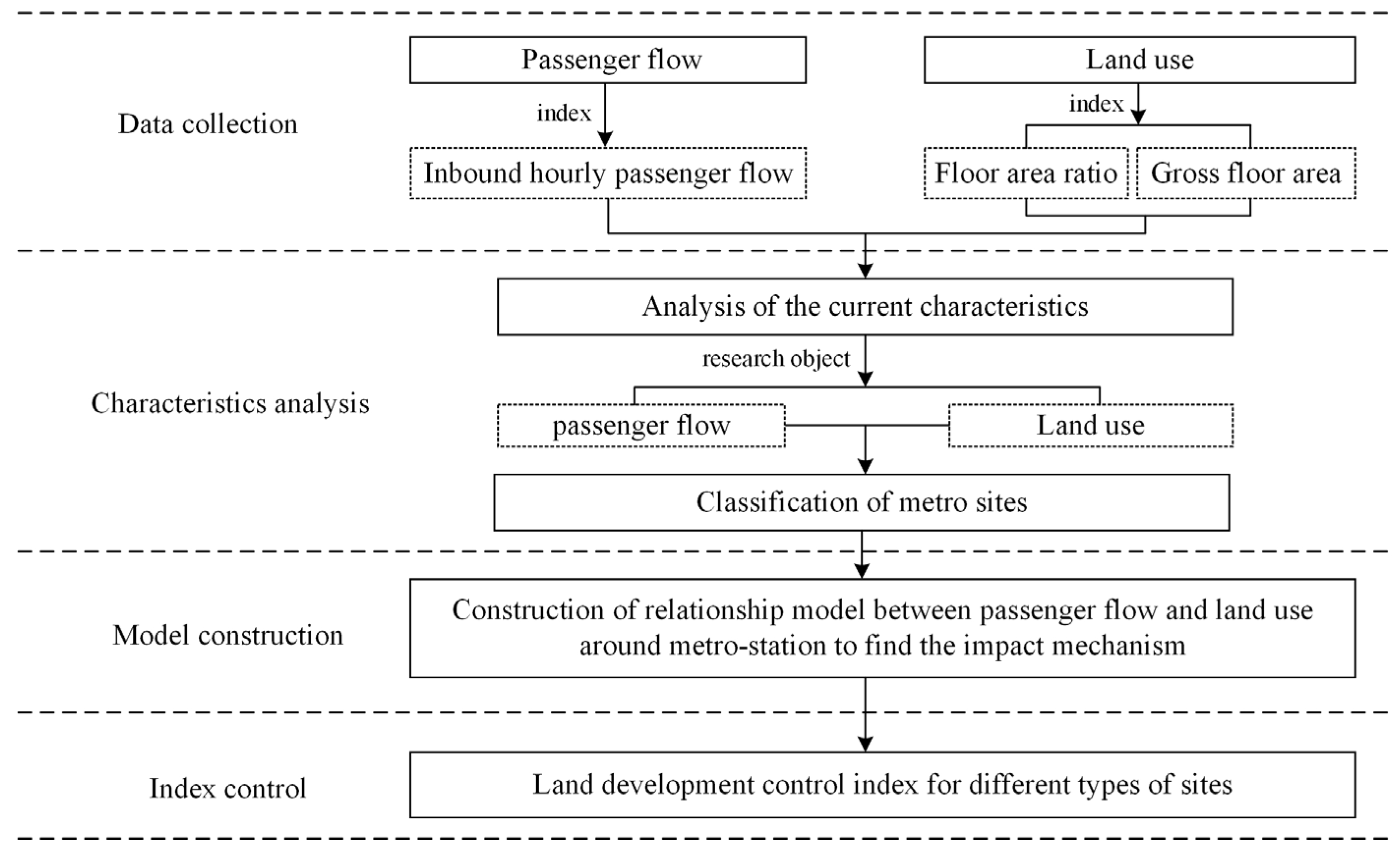
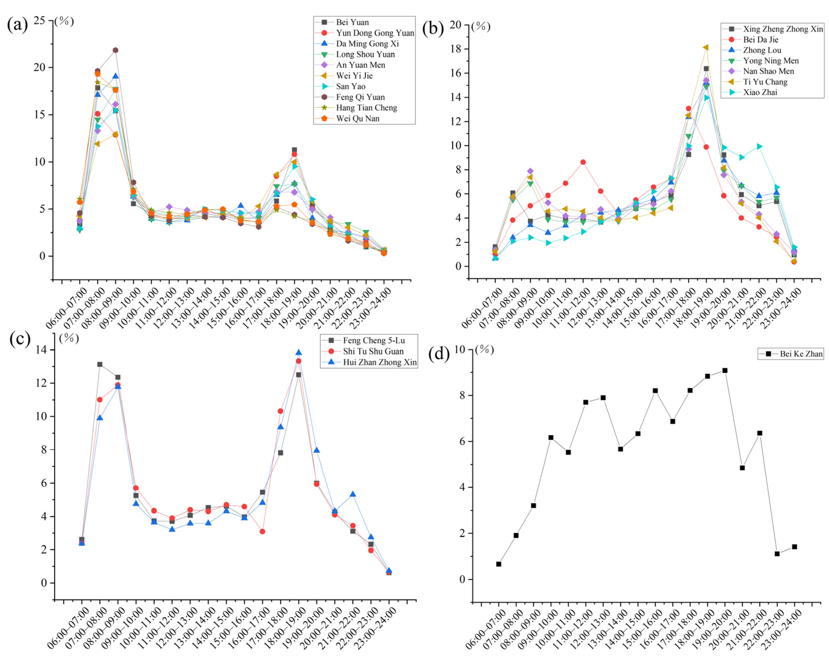
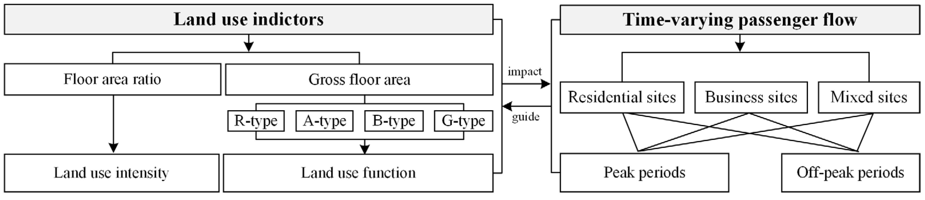
- Classification of metro sites. According to the characteristics of land use around the station at present, and the time-varying law of the hourly coefficient on weekdays, the metro sites were classified into several types. Based on the site classification, a specific period division to vary the time periods was proposed.
- Impact mechanism of land use on hourly flow at various stations. Based on the independent variable types determined after applying the Pearson parameter dimensionality reduction, a linear regression model connecting the hourly flow with different land use indicators was constructed for different periods.
- Land use control for different types of sites. According to the fitting equation through the multiple linear regression model, the maximum values of the floor area ratio and gross floor area were proposed.
- 1.
- Land use mixture
- 2.
- Hourly coefficient
- 3.
- Pearson correlation coefficient
- 4.
- Multiple linear regression model
- 5.
- Mean absolute percentage error
- 6.
- To test the reliability of the fitting equation, the mean absolute percentage error (MAPE) was calculated using Equation (5). This formula was used in this study to measure the difference between the actual and fitted flow. If the value is less than 30%, the fitting equation is valid.
3. Results and Discussion
3.1. Site Classification
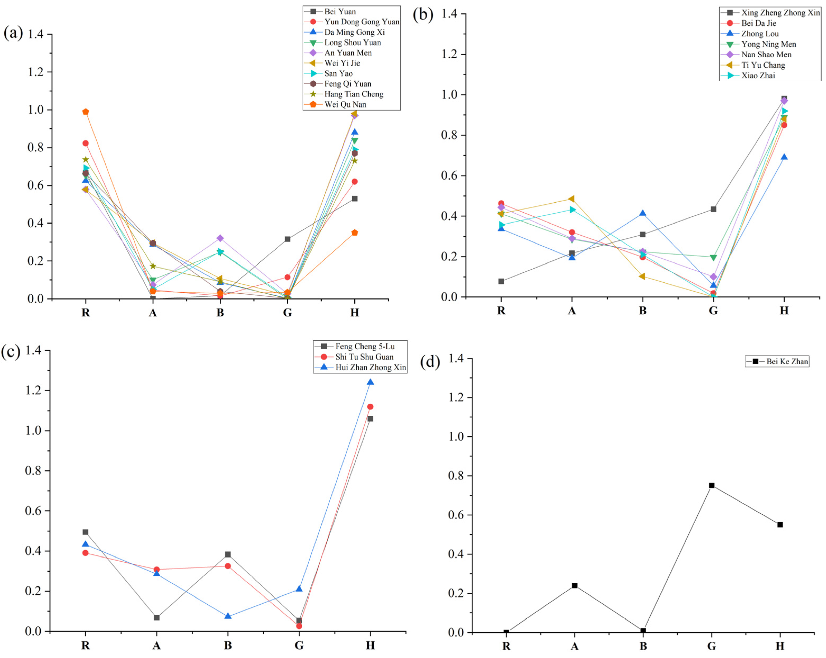
3.2. Impact of Floor Area Ratio on Hourly Flow
3.3. Impact of Gross Floor Area on Hourly Flow
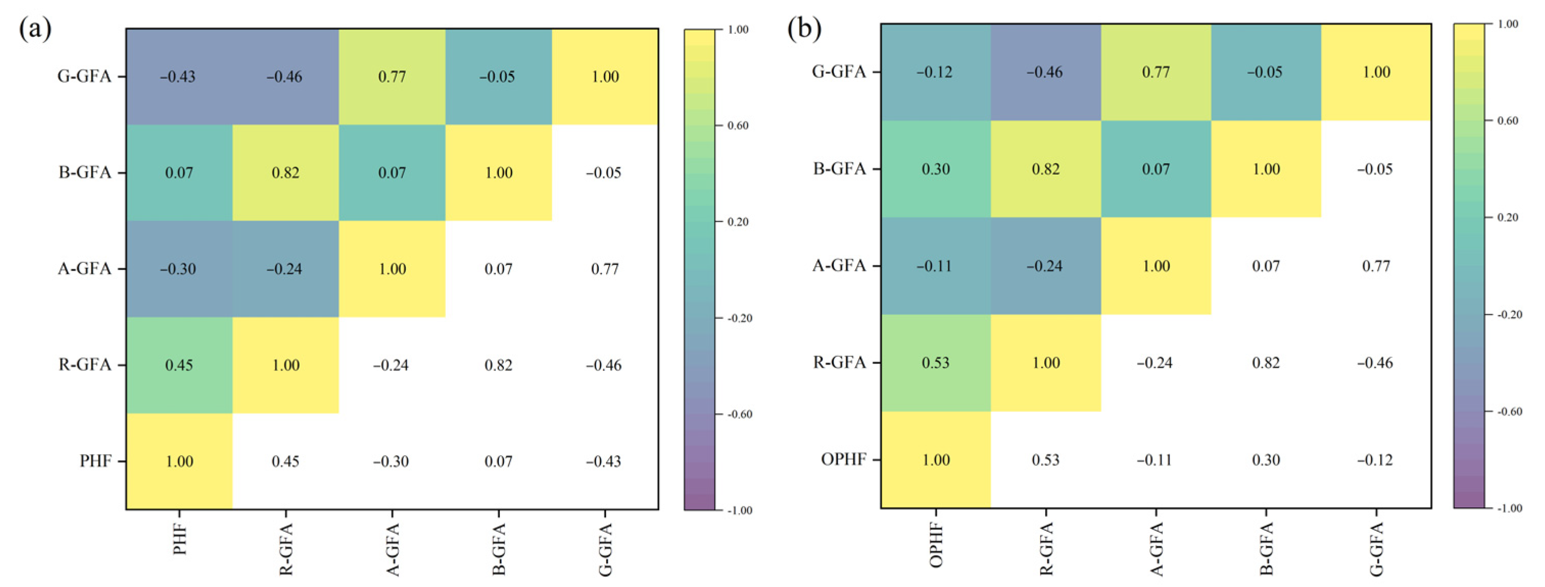
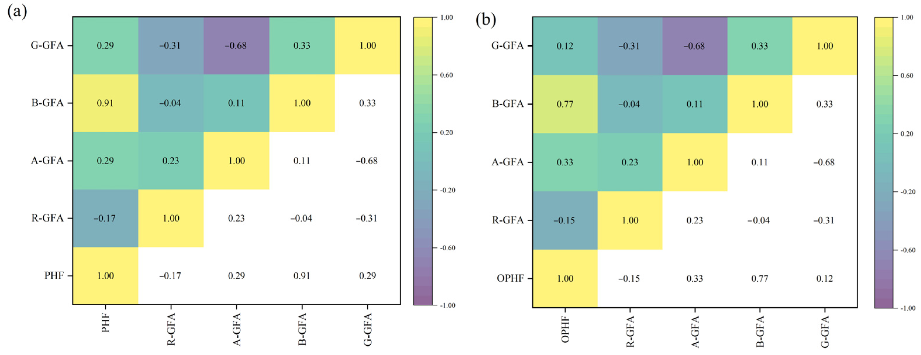
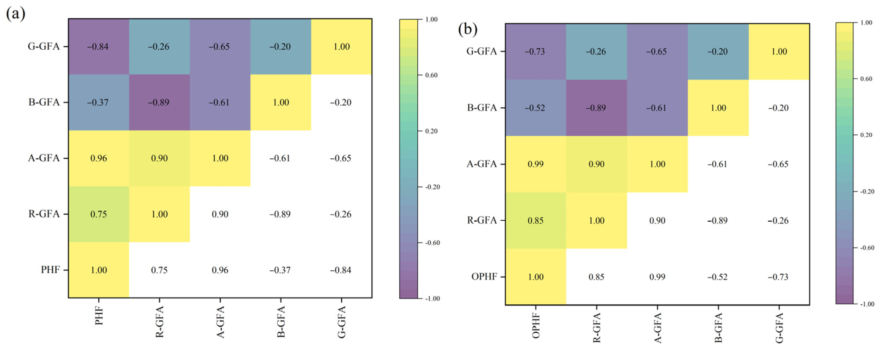
3.3.1. Pearson Correlation
- 7.
- Residential Sites
- 8.
- Business Sites
- 9.
- Mixed sites
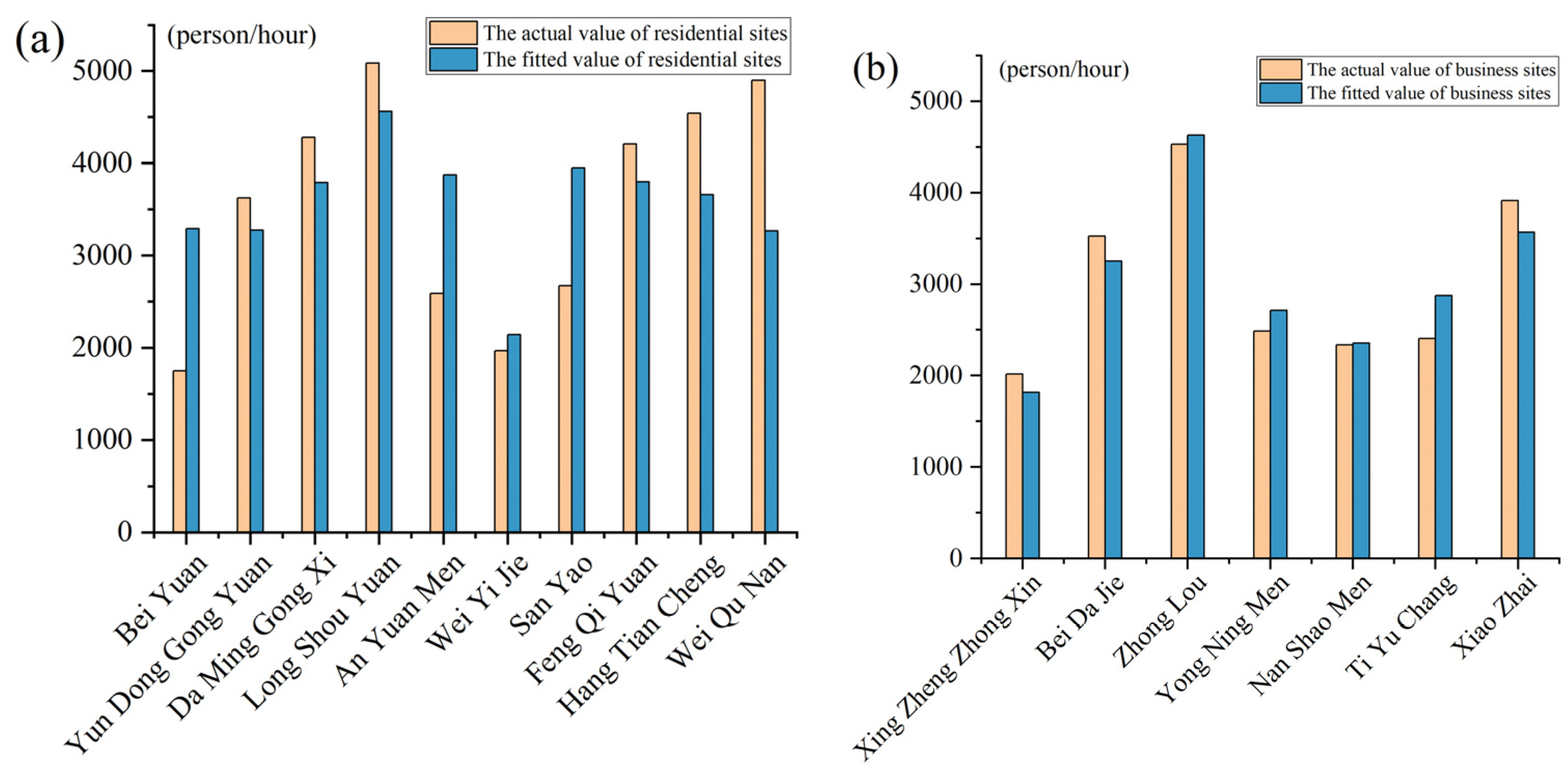
3.3.2. Impact Intensity
- 10.
- Peak periods
- 11.
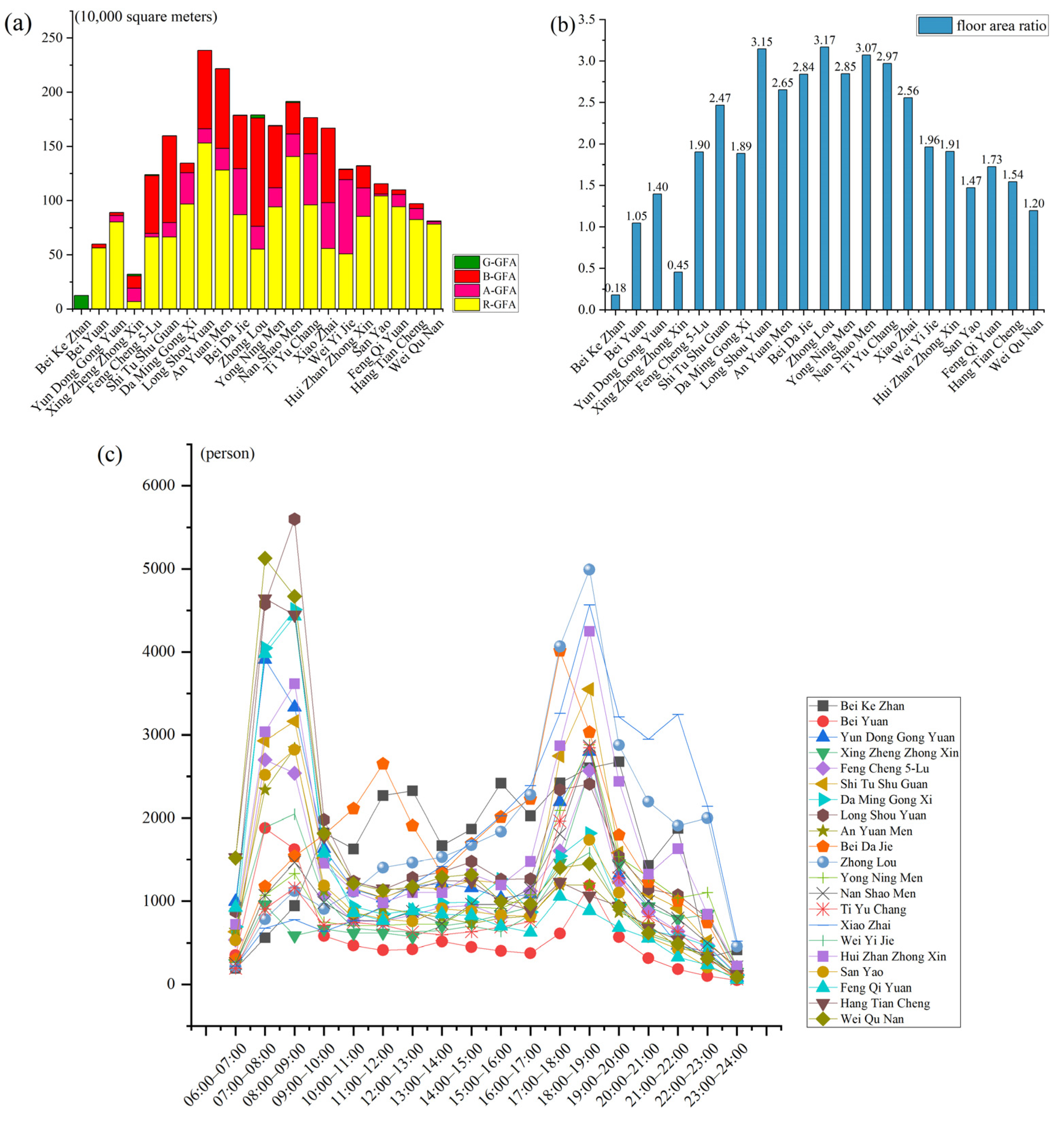
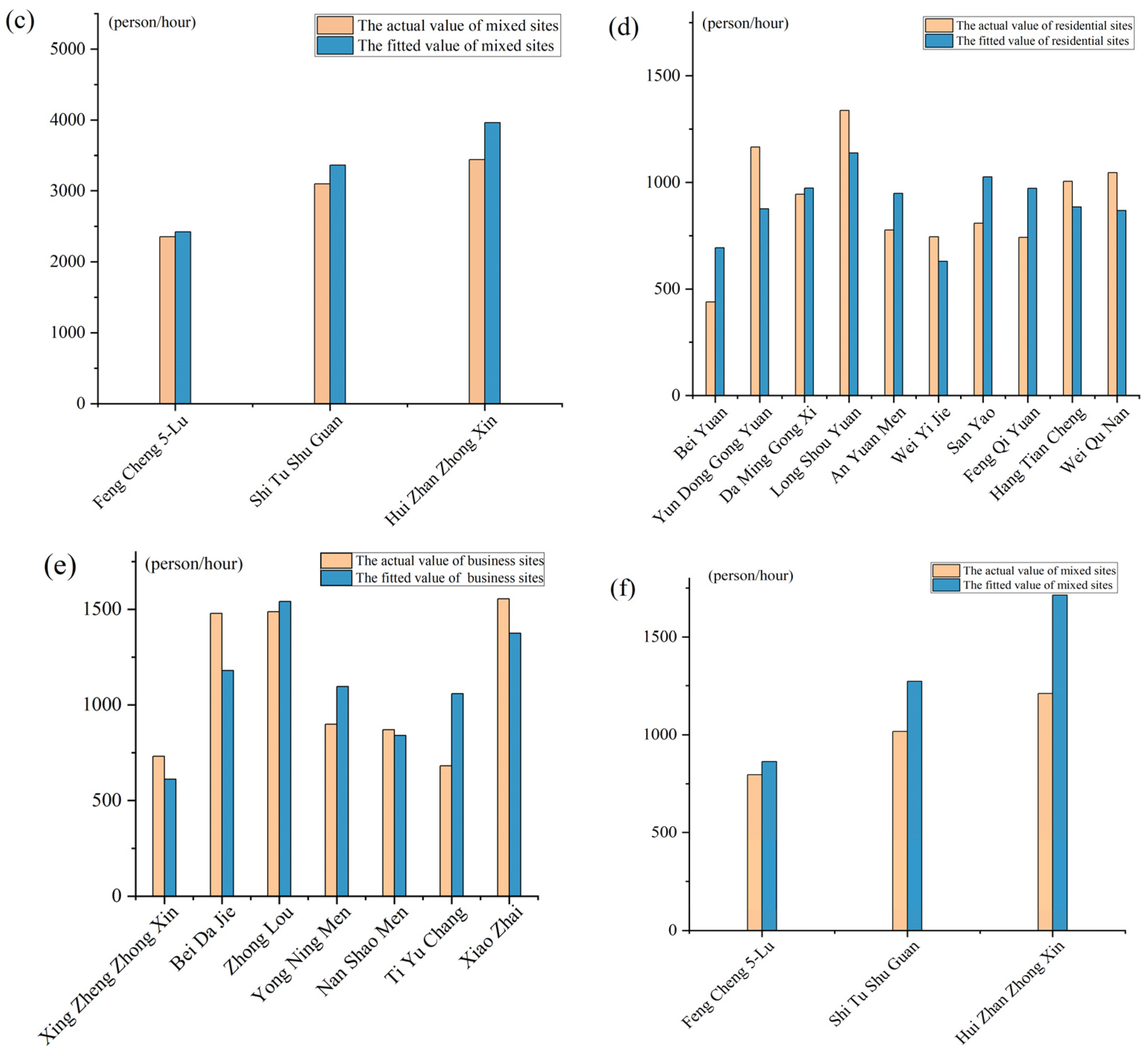
- The results presented above indicate that the inbound flow originates from regions with different land use types. During the peak periods, R-type land around residential sites provided the majority of the flow due to the high number of people traveling to work, and the peak times for mixed sites was the result of people commuting on weekdays. B-type land around the business sites provided the majority of the flow as individuals were returning to their accommodation [51,52]. Notably, the lower R and R2 of the PHF and GFAs that are fit for residential sites may have been due to the fact that during weekday peak hours, other factors have a greater impact on the flow because of the requirements for compressed commuting times; for instance, residents may consider whether to transfer, bus stop density, and so on. These factors create a strong interference with the dependent variable, thus resulting in a slightly lower fitting effect of R-GFA, A-GFA, and G-GFA on passenger flow.
- 12.
- Off-peak periods
3.4. Land Development Control
- Residential sites
- Business sites
- Mixed sites
4. Conclusions
- The emergence of extreme passenger flow at metro stations was influenced by a number of complex factors, including the built environment of the station area; therefore, there were some limitations to this study. In particular, spatial factors other than land use were not considered, and the sample size was small, as only line 2 was considered for the study. Finally, the presented study failed to consider the spatial variability of station distribution; therefore, subsequent studies should be improved in the following three ways:
- More consideration should be given to the factors concerning the built environment that impact passenger flow at the station, including the distribution of public stations, the amount of parking, and the quality of the pedestrian environment, so that extreme passenger flow can be more accurately and effectively managed to ensure public safety.
- The diversity of the study sites can further improve the accuracy of the results; therefore, the number and type of sample sites needs to be expanded in future studies. For example, all 116 sites within the main city of Xi’an could be selected for the study.
- The GWR and GTWR models consider the spatial variability of different sites, and therefore, they have the advantage of being more accurate. Further research can introduce spatial parameters through these models to propose more reasonable diversified development strategies for different types of sites.
Author Contributions
Funding
Data Availability Statement
Acknowledgments
Conflicts of Interest
References
- Atkinson-Palombo, C.; Kuby, M.J. The geography of advance transit-oriented development in metropolitan Phoenix, Arizona, 2000–2007. J. Transp. Geogr. 2011, 19, 189–199. [Google Scholar] [CrossRef]
- Zegras, C. Land Use and Transport in China. J. Transp. Land Use 2010, 3, 1–3. [Google Scholar] [CrossRef] [Green Version]
- Choi, J.; Lee, Y.; Kim, T.; Sohn, K. An analysis of metro ridership at the station-to station level in Seoul. Transportation 2012, 39, 705–722. [Google Scholar] [CrossRef]
- Shi, J.G.; Yang, J.; Yang, L.X. Safety-oriented cooperative passenger flow control model in peak hours for a metro line. J. Transp. Syst. Eng. Inf. Technol. 2019, 19, 125–131. [Google Scholar]
- Truong, R.; Gkountouna, O.; Pfoser, D.; Züfle, A. Towards a Better Understanding of Public Transportation Traffic: A Case Study of the Washington, DC Metro. Urban Sci. 2018, 2, 65. [Google Scholar] [CrossRef] [Green Version]
- Wang, K.; Zhang, J.J.; Zhang, D.; Wu, X. A priority in land supply for sustainable transportation of Chinese cities: An empirical study from perception, discrimination, linkage to decision. Land 2022, 11, 78. [Google Scholar] [CrossRef]
- Cao, X.S.; Yang, F.; Xiao-Pei, Y. Study on the urban transport and land-use of Guangzhou. Chin. Geogr. Sci. 2000, 2, 144–150. [Google Scholar] [CrossRef]
- Hou, Q.H.; Duan, Y.Q.; Ma, R.G. Collaborative optimization of land use intensity and traffic capacity under hierarchical control rules of regulatory detailed planning. J. Chang’an Univ. 2015, 35, 114–121. [Google Scholar]
- Moon, Y.I.; Rho, J.H. An empirical analysis on public transportation demand and TOD design factors in Seoul subway adjacent area. Int. J. Highw. Eng. 2011, 13, 211–220. [Google Scholar] [CrossRef] [Green Version]
- Knight, R.L.; Trygg, L.L. Land use impacts of rapid transit: Implications of recent experience. Energy Plan. Policy Econ. 1977. [Google Scholar] [CrossRef] [Green Version]
- Werner, C. Integrated land-use and transport modeling-Decision chains and hierarchies—Delabarra, T. Environ. Plan. B Plan. Des. 1990, 19, 487–490. [Google Scholar]
- Zhao, L.; Shen, L. The impacts of rail transit on future urban land use development: A case study in Wuhan, China. Transp. Policy 2018, 81, 396–405. [Google Scholar] [CrossRef]
- Kuby, M.; Barranda, A.; Upchurch, C. Factors influencing light-rail station boardings in the United States. Transp. Res. Part A Policy Pract. 2004, 38, 223–247. [Google Scholar] [CrossRef]
- Cervero, R.; Kockelman, K. Travel demand and the 3ds: Density, diversity, and design. Transp. Res. Part D Transp. Environ. 1997, 2, 199–219. [Google Scholar] [CrossRef]
- Voulgaris, C.T.; Blumenberg, E.; Taylor, B.D.; Brown, A.; Ralph, K.M. Neighborhood Character and Travel Behavior: Comprehensive Analysis of the United States in the 2000s. In Proceedings of the Transportation Research Board 95th Annual Meeting, Washington, DC, USA, 8–12 January 2016. [Google Scholar]
- Teng, S.H. Analysis of the relationship between land use, development, and construction near a rail traffic station and passenger flow volume: The case of Tianjin metro line 1. Appl. Mech. Mater. 2013, 357–360, 1856–1862. [Google Scholar] [CrossRef]
- Wu, H.; Gao, L. Functional analysis of passenger flow at rail transit in Beijing based on the usage of land. J. Beijing Univ. Civ. Eng. Archit. 2015, 31, 28–35. [Google Scholar]
- Zhang, Y.; Cao, K.; He, Y.W.; Zhou, W. Discussion on spatial match between land use and rail transit: A case study of Shenzhen subway line 2. City Plan. Rev. 2017, 41, 107–115. [Google Scholar]
- Lewis-Workman, S.; Brod, D. Measuring the neighborhood benefits of rail transit accessibility. Transp. Res. Rec. J. Transp. Res. Board 1997, 1, 147–153. [Google Scholar] [CrossRef] [Green Version]
- Zhuang, Y.; Yuan, M. An analysis on the influence of passenger flow on development intensity in metro station area in the core area of downtown shanghai. Archit. J. 2017, 2, 22–26. [Google Scholar]
- Yoshiharu, S. Factors in expansion of low-use and unused land in core areas of regional centers: Comparative study between Matsuyama city and Takamatsu city. Geogr. Sci. 2007, 62, 65–78. [Google Scholar]
- Chen, X. Driving Factors Analysis on Urban Vibrancy: A Case Study of Chongqing Main Area; Springer: Singapore, 2021; pp. 1137–1147. [Google Scholar]
- Sung, H.; Choi, K.; Lee, S.; Cheon, S.H. Exploring the impacts of land use by service coverage and station-level accessibility on rail transit ridership. J. Transp. Geogr. 2014, 36, 134–140. [Google Scholar] [CrossRef]
- Duan, Y.Q.; Hou, Q.H.; Zhang, S.Y. Review of intensive land use in built-up area based on low-carbon travel. Planners 2019, 35, 5–11. [Google Scholar]
- Cynthia, C.; Jason, C.; James, B. Diurnal pattern of transit ridership: A case study of the new york city subway system. J. Transp. Geogr. 2009, 17, 176–186. [Google Scholar]
- Ding, C.; Cao, X.Y.; Liu, C. How does the station-area Build environment influence metro rail ridership? Using gradient boosting decision trees to identify non-linear threshold. J. Transp. Geogr. 2019, 77, 70–78. [Google Scholar] [CrossRef]
- Mo, Y.K.; Deng, J.; Wang, J.Y. A land use model for urban rail station area planning based on Tod strategy. J. Civ. Archit. Environ. Eng. 2009, 31, 116–120. [Google Scholar]
- Wang, J.Y.; Zheng, X.; Yikui, M.O. Establishment of density zoning and determination of plot ratio along rail transit line based on TOD: A case study on rail transit line 3 in Shenzhen. City Plan. Rev. 2011, 4, 30–35. [Google Scholar]
- Zhang, W.; Long, C.P. Determination of plot ratio surrounding rail transit station—A case of YuanYang station on Chongqing light rail transit. Urban Mass Transit. 2017, 01, 91–95. [Google Scholar]
- Tang, X.L.; Huang, Z.D.; Lin, M. The characteristics of urban rail transit and its relationship with land use in Shenzhen. Urban Rural Plan. 2018, 03, 98–104. [Google Scholar]
- Chang, L.Y.; Lin, D.J. Analysis of international air passenger flows between two countries in the APEC region using non-parametric regression tree models. Lect. Notes Eng. Comput. Sci. 2010, 2180, 415–420. [Google Scholar]
- Su, H.L.; Wang, Y.; Wang, X.; Zhou, R. Transit-oriented development correlates of rail transit ridership in shanghai municipality. J. Tongji Univ. 2014, 42, 71–77. [Google Scholar]
- Yuankun, L.; Xiafei, Y. The relationship between the scale of urban rail transit network and population and post density. Urban Rail Transit Res. 2017, 20, 10–14. [Google Scholar]
- Gu, J.C. Relationship between ridership characteristics at railway stations and surrounding land-use in Shenzhen. Traffic Transp. 2019, 35, 47–50. [Google Scholar]
- Duan, Y.; Lei, K.; Tong, H.; Li, B.; Hou, Q.H. Land use characteristics of Xi’an residential blocks based on pedestrian traffic system. Alex. Eng. J. 2021, 60, 15–24. [Google Scholar] [CrossRef]
- Moniruzzaman, M.; Páez, A. Accessibility to transit, by transit, and mode share: Application of a logistic model with spatial filters. J. Transp. Geogr. 2012, 24, 198–205. [Google Scholar] [CrossRef]
- Loo, B.P.; Chen, C.; Chan, E.T. Rail-based transit-oriented development: Lessons from New York City and Hong Kong. Land Sc. Urban Plan. 2010, 97, 202–212. [Google Scholar] [CrossRef]
- Cervero, R. Alternative approaches to modeling the travel-demand impacts of smart growth. J. Am. Plan. Assoc. 2006, 72, 285–295. [Google Scholar] [CrossRef]
- Wei, Z.Y.; Su, H.M.; Huang, R.J. The influence of the construction of Xi’an Metro Line 2 on land use change. Chin. J. Ecol. 2018, 37, 2474–2482. [Google Scholar]
- Kim, H.; Nam, J. The size of the station influence area in Seoul, Korea: Based on the survey of users of seven stations. Int. J. Urban Sci. 2013, 17, 331–349. [Google Scholar] [CrossRef]
- Jin, D.; Meng, X. Characteristics of subway station ridership with surrounding land use: A case study in Beijing. In Proceedings of the 2015 International Conference on Transportation Information and Safety (ICTIS), Wuhan, China, 25–28 June 2015; pp. 330–336. [Google Scholar]
- GB/T 50137-2011; Code for Classification of Urban Land Use and Planning Standards of Development Land. Ministry of Housing and Urban-Rural Development of the People’s Republic of China: Beijing, China, 2012.
- Tang, T. Development control, planning incentive and urban redevelopment: Evaluation of a two-tier plot ratio system in Hong Kong. Land Use Policy 1999, 16, 33–43. [Google Scholar] [CrossRef]
- Feng, H.; Zhang, S. Study on travel efficiency and land use mixing degree based on meta fractal dimension theory. J. Xi’an Univ. Archit. Technol. 2014, 46, 882–887. [Google Scholar]
- Ye, X.F.; Ming, R.L.; Li, R.X. Rail transit in Tokyo and Seoul: Development trends & characteristics of passenger flow. Urban Transp. China 2008, 6, 16–20. [Google Scholar]
- Jin, Y. The influence of l and use on diurnal pattern of urban mass transit station boardings: A case study of shanghai city. Mod. Urban Res. 2015, 6, 13–19. [Google Scholar]
- Li, J.B.; Cui, Y. Research on relationship between passenger flow and attraction of surrounding land on Tianjin metro line 1 based on cell phone signaling data. Urban Passeng. Transp. 2019, 6, 50–56. [Google Scholar]
- Xia, F.S.; Chen, H.; Yuan, J.M.; Zhang, K.; Zhang, K. Research on automatic detection method of building in aerial stereo image based on elevation constraints. Geogr. Geo-Inf. Sci. 2019, 35, 46–50. [Google Scholar]
- Chen, W.G. The Discussion of Rational Exploitation Strength in the Plot around the Metro Station: Starting with the Detailed Plan of Rail Transport in Second Phase in Shenzhen. Mod. Urban Res. 2006, 08, 44–50. [Google Scholar]
- Yao, J.T.; Dong, Z.P. Correlativity of random variables and structural reliability. J. Xi’an Univ. Archit. Technol. 2000, 32, 114–118. [Google Scholar]
- Cui, Y.C.; Guan, H.Z.; Yang, S.I.; Qin, Z.T. Residents’ travel characteristics based on order data of on-line car-hailing: A case study of Beijing. Transp. Res. 2018, 4, 20–28. [Google Scholar]
- Zhuang, C.T.; Wu, C.C.; Gu, T.Q.; Li, J. Analysis on characteristics of rail transit and conventional bus transfer in Suzhou. Traffic Transp. 2021, 37, 51–55. [Google Scholar]
- Zheng, W.H. Discussion on land use layout of residential rail transit station areas. Planners 2009, 025, 58–62. [Google Scholar]
- Cui, X.; Yu, B.J.; Liang, P.P.; Wang, L.; Zhang, L.F. Urban rail transit station type identification and job-housing spatial rebalancing based on passenger flow and land use: Taking Chengdu as an example. Mod. Urban Res. 2021, 36, 68–79. [Google Scholar]
- Kittelson, Associates Inc. TRB’s Transit Cooperative Research Program (TCRP) Report 100: Transit Capacity and Quality of Service Manual, 2nd ed.; Transportation Research Board|National Academies: Washington, DC, USA, 2003. [Google Scholar]
- GB/T 50157-2013; Metro Design Specification. China Architecture and Building Press: Beijing, China, 2013.


| Data Categories | Index | Significance | Sources | Unit |
|---|---|---|---|---|
| Land use | Floor area ratio (FAR) | Land develop-ment intensity | maps.google.com GIS database field research | / |
| Gross floor area (GFA) | Land development function | maps.google.com GIS database field research | m2 | |
| Passenger flow | Hourly flow | Passenger flow per hour | AFC system | person/hour |
| Type | Station(s) | Number |
|---|---|---|
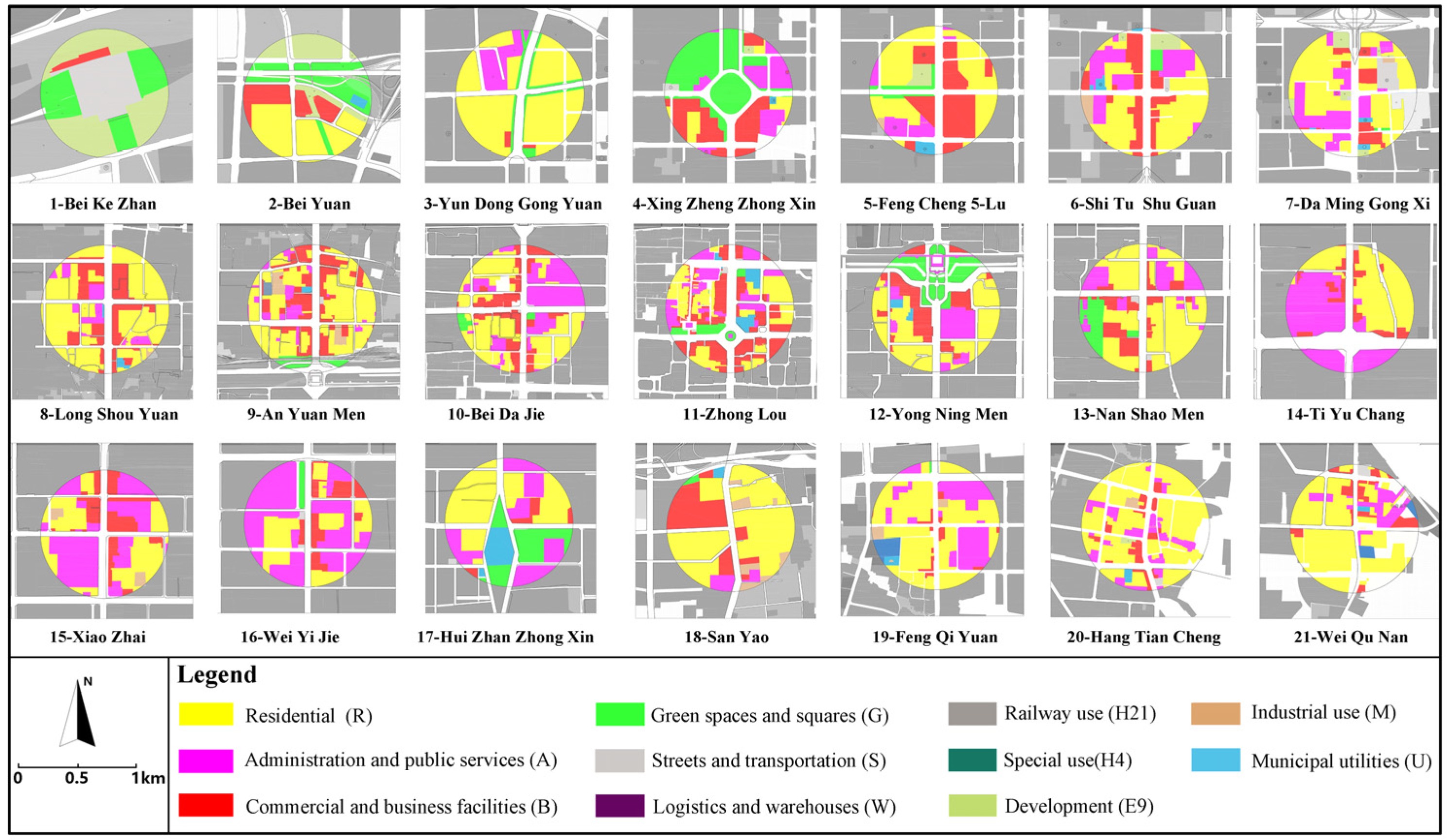
| Residential 1 | Bei Yuan, Yun Dong Gong Yuan, Da Ming, Gong Xi, Long Shou Yuan, An Yuan Men, Wei Yi Jie, San Yao, Feng Qi Yuan, Hang Tian Cheng, and Wei Qu Nan | 10 |
| Business 2 | Xing Zheng Zhong Xin, Bei Da Jie, Zhong Lou, Yong Ning Men, Nan Shao Men, Ti Yu Chang, and Xiao Zhai | 7 |
| Mixed 3 | Feng Cheng 5-Lu, Shi Tu Shu Guan, and Hui Zhan Zhong Xin | 3 |
| Traffic 4 | Bei Ke Zhan | 1 |
| Residential | Business | Mixed | |||||||
|---|---|---|---|---|---|---|---|---|---|
| a | Constant | k | a | Constant | k | a | Constant | k | |
| Y1 | 403.46 | 2841.24 | 0.21 | 422.36 | 1961.39 | 0.41 | 331.99 | 2284.76 | 0.20 |
| Y2 | 167.40 | 602.56 | 0.42 | 136.18 | 755.26 | 0.33 | 15.14 | 976.63 | 0.23 |
| Types of Sites | Residential | Business | Mixed |
|---|---|---|---|
| Peak hourly flow | R, A, G | A, B, G | A, B, G |
| Off-Peak hourly flow | R, B | A, B | A, B, G |
| R | R2 | Adjusted R2 | Standard Error | Sig. |
|---|---|---|---|---|
| 0.54 | 0.51 | 0.48 | 1286.51 | 0.03 |
| Non-Standard Coefficient | Standard Coefficient | T | Sig. | ||
|---|---|---|---|---|---|
| Model | B | Standard Error | Beta | ||
| 2613.14 | 593.96 | 4.40 | 0.02 | ||
| R-GFA | 12.82 | 1.25 | 0.32 | 10.29 | 0.00 |
| A-GFA | −0.99 | 0.17 | −0.02 | −5.82 | 0.01 |
| G-GFA | −2512.61 | 592.98 | −0.27 | −4.32 | 0.02 |
| R | R2 | Adjusted R2 | Standard Error | Sig. |
|---|---|---|---|---|
| 0.95 | 0.91 | 0.81 | 413.65 | 0.04 |
| Non-standard Coefficient | Standard Coefficient | T | Sig. | ||
|---|---|---|---|---|---|
| Model | B | Standard Error | Beta | ||
| 609.90 | 143.51 | 4.25 | 0.03 | ||
| A-GFA | 31.13 | 6.90 | 0.47 | 4.51 | 0.02 |
| B-GFA | 23.88 | 7.26 | 0.73 | 3.29 | 0.04 |
| G-GFA | 360.54 | 62.70 | 0.37 | 5.75 | 0.01 |
| R | R2 | Adjusted R2 | Standard Error | Sig. |
|---|---|---|---|---|
| 0.73 | 0.62 | 0.56 | 413.65 | 0.02 |
| Non-standard Coefficient | Standard Coefficient | T | Sig. | ||
|---|---|---|---|---|---|
| Model | B | Standard Error | Beta | ||
| 4077.70 | 959.50 | 4.24 | 0.03 | ||
| A-GFA | 20.15 | 1.78 | 0.87 | 11.34 | 0.00 |
| B-GFA | −10.39 | 3.05 | −0.41 | −3.41 | 0.04 |
| G-GFA | −1244.61 | 216.93 | −0.33 | −5.74 | 0.01 |
| R | R2 | Adjusted R2 | Standard Error | Sig. |
|---|---|---|---|---|
| 0.59 | 0.45 | 0.43 | 232.17 | 0.03 |
| Non-Standard Coefficient | Standard Coefficient | T | Sig. | ||
|---|---|---|---|---|---|
| Model | B | Standard Error | Beta | ||
| 289.60 | 45.67 | 6.34 | 0.02 | ||
| R-GFA | 7.43 | 0.82 | 0.90 | 9.06 | 0.01 |
| B-GFA | −3.99 | 0.78 | −0.45 | −5.12 | 0.03 |
| R | R2 | Adjusted R2 | Standard Error | Sig. |
|---|---|---|---|---|
| 0.80 | 0.65 | 0.47 | 283.13 | 0.02 |
| Non-Standard Coefficient | Standard Coefficient | T | Sig. | ||
|---|---|---|---|---|---|
| Model | B | Standard Error | Beta | ||
| 417.66 | 42.10 | 9.92 | 0.01 | ||
| A-GFA | 6.63 | 0.31 | 0.24 | 21.39 | 0.00 |
| B-GFA | 9.83 | 2.05 | 0.74 | 4.79 | 0.04 |
| R | R2 | Adjusted R2 | Standard Error | Sig. |
|---|---|---|---|---|
| 0.95 | 0.89 | 0.88 | 416.22 | 0.03 |
| Non-Standard Coefficient | Standard Coefficient | T | Sig. | ||
|---|---|---|---|---|---|
| Model | B | Standard Error | Beta | ||
| 1453.02 | 429.50 | 3.38 | 0.04 | ||
| A-GFA | 19.25 | 3.23 | 0.84 | 5.96 | 0.01 |
| B-GFA | −4.81 | 1.09 | −0.53 | −4.42 | 0.03 |
| G-GFA | −426.41 | 96.93 | −0.29 | −4.40 | 0.03 |
| Periods | Residential | Business | Mixed | |||
|---|---|---|---|---|---|---|
| Peak | Off-Peak | Peak | Off-Peak | Peak | Off-Peak | |
| MAPE (%) | 28 | 22 | 8 | 19 | 8 | 25 |
| Site Type | FAR | GFA (One Unit: 10,000 m2) |
|---|---|---|
| Residential sites | 5.3 | 204.68(R-GFA) |
| Business sites | 7.2 | 132.29(B-GFA) |
| Mixed sites | 8.2 | 101.19(A-GFA) |
Publisher’s Note: MDPI stays neutral with regard to jurisdictional claims in published maps and institutional affiliations. |
© 2022 by the authors. Licensee MDPI, Basel, Switzerland. This article is an open access article distributed under the terms and conditions of the Creative Commons Attribution (CC BY) license (https://creativecommons.org/licenses/by/4.0/).
Share and Cite
Lei, K.; Hou, Q.; Li, W.; Zhao, M.; Zhou, J.; Zhang, L.; Chen, S.; Duan, Y. The Impact of Land Use on Time-Varying Passenger Flow Based on Site Classification. Land 2022, 11, 2189. https://doi.org/10.3390/land11122189
Lei K, Hou Q, Li W, Zhao M, Zhou J, Zhang L, Chen S, Duan Y. The Impact of Land Use on Time-Varying Passenger Flow Based on Site Classification. Land. 2022; 11(12):2189. https://doi.org/10.3390/land11122189
Chicago/Turabian StyleLei, Kexin, Quanhua Hou, Weijia Li, Meng Zhao, Jizhe Zhou, Lingda Zhang, Shihan Chen, and Yaqiong Duan. 2022. "The Impact of Land Use on Time-Varying Passenger Flow Based on Site Classification" Land 11, no. 12: 2189. https://doi.org/10.3390/land11122189