
Modelling Floodplain Vegetation Response to Groundwater Variability Using the ArcSWAT Hydrological Model, MODIS NDVI Data, and Machine Learning

Abstract
:1. Introduction
2. Materials and Methods
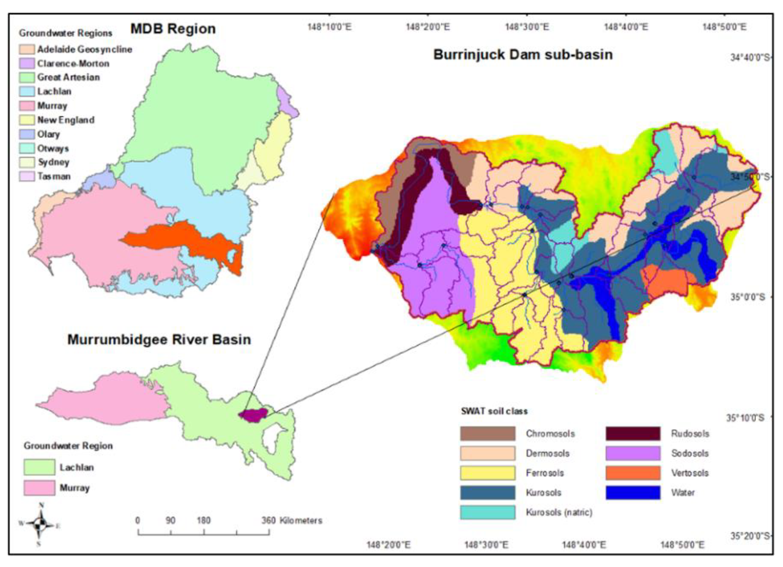
2.1. Study Area
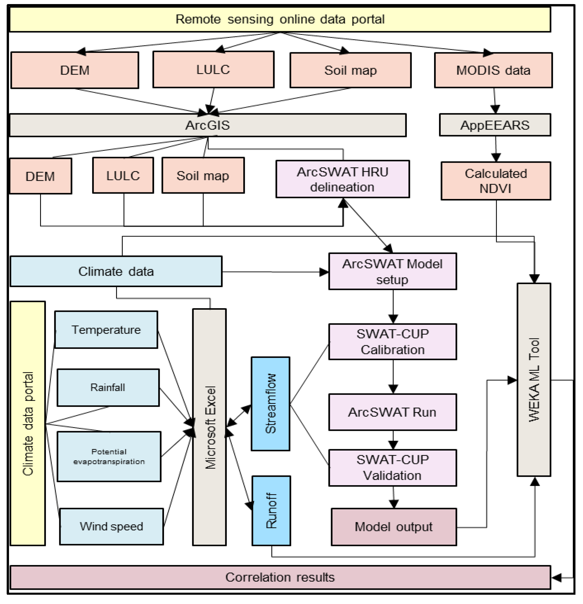
2.2. Methods
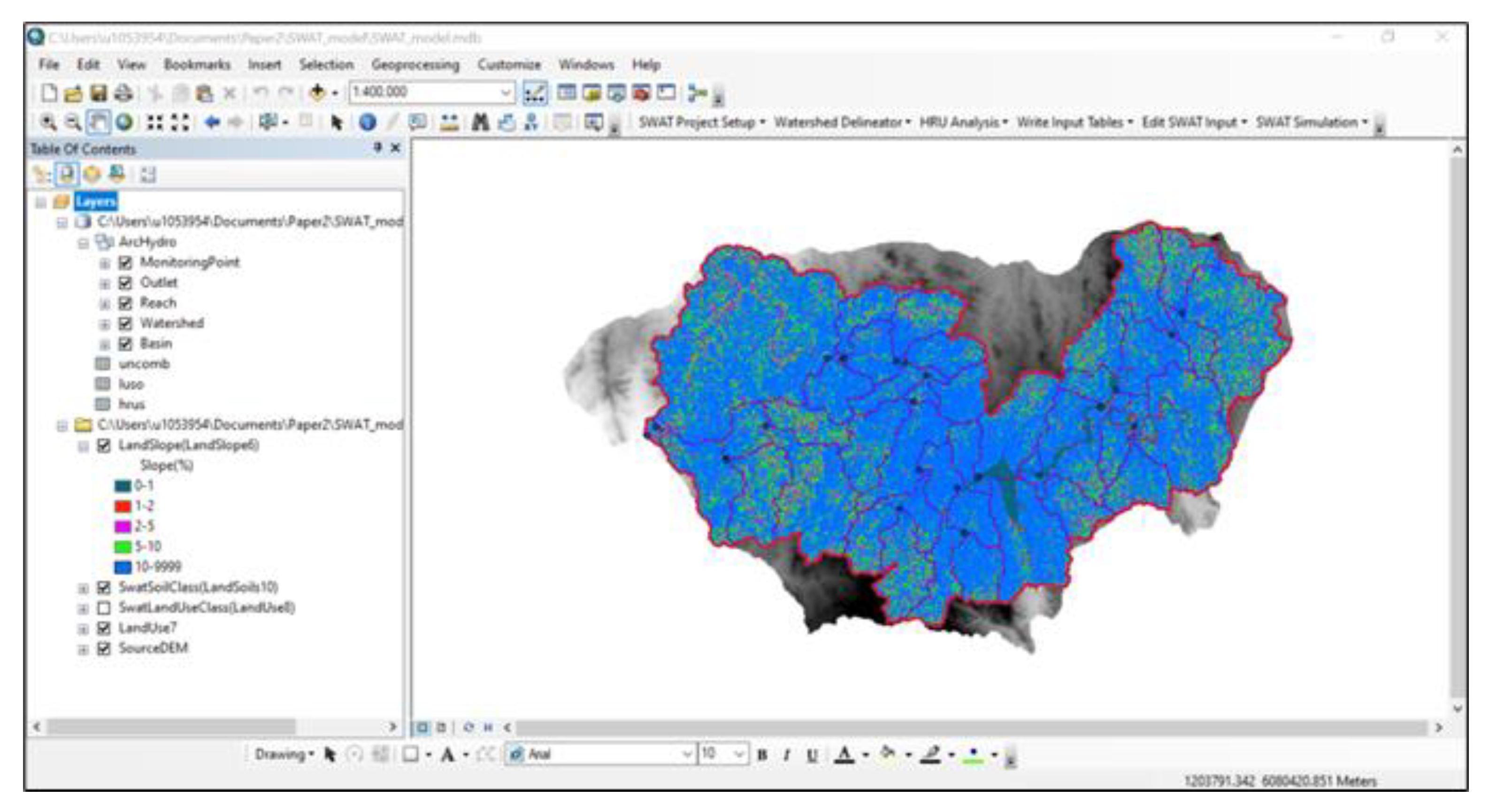
2.3. Hydrological Model Setup
2.3.1. Data Preparation
2.3.2. Study Period
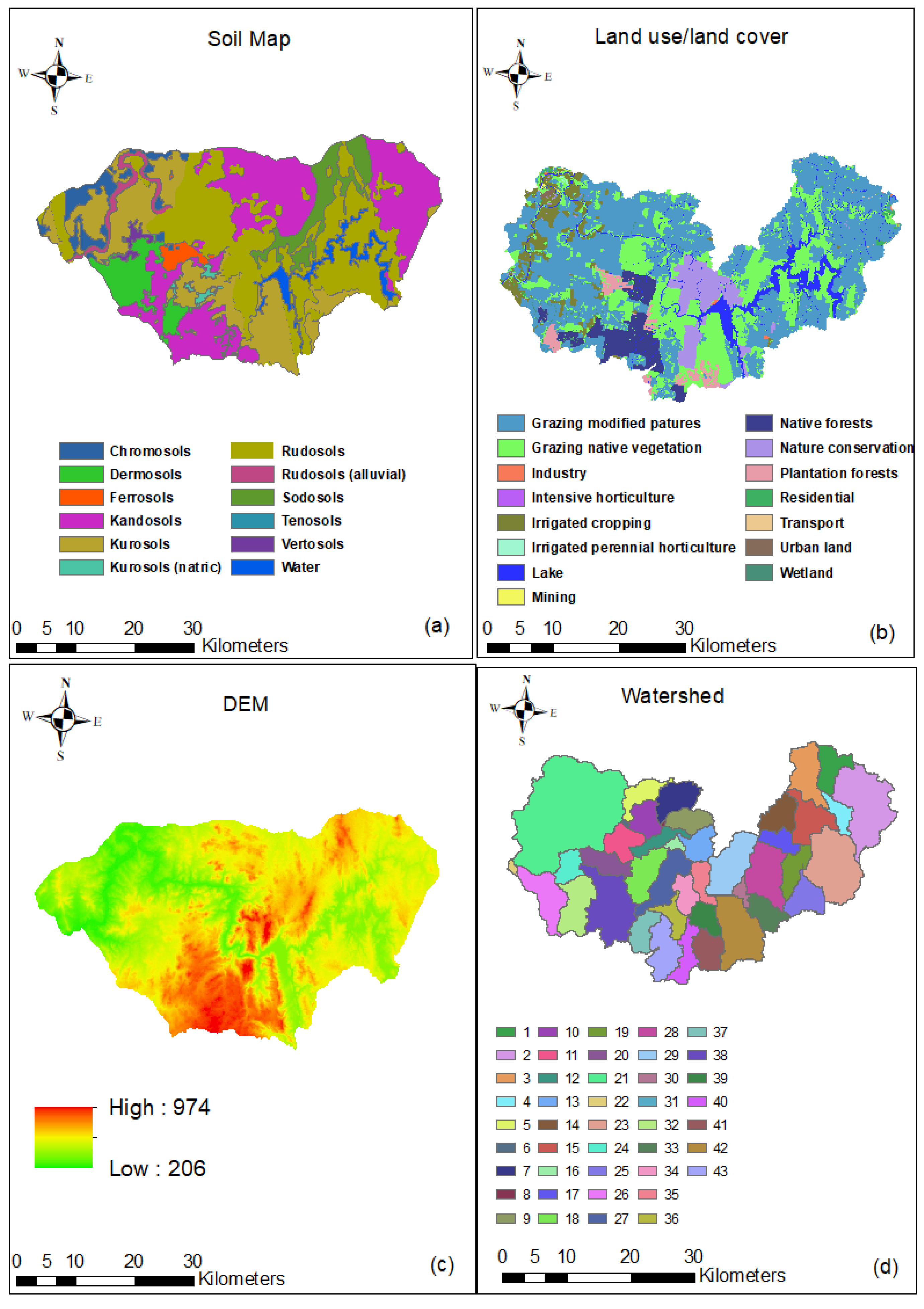
2.3.3. DEM
2.3.4. Land Use/Land Cover Data
2.3.5. Soil Data
2.3.6. Climate Data
2.3.7. Sensitivity Analysis and Hydrological Model Calibration
2.3.8. Hydrological Model Performance Evaluation
2.3.9. Remote Sensing Data
2.3.10. Normalised Difference Vegetation Index (NDVI)
2.3.11. Machine Learning Algorithms for Data Analysis
3. Results
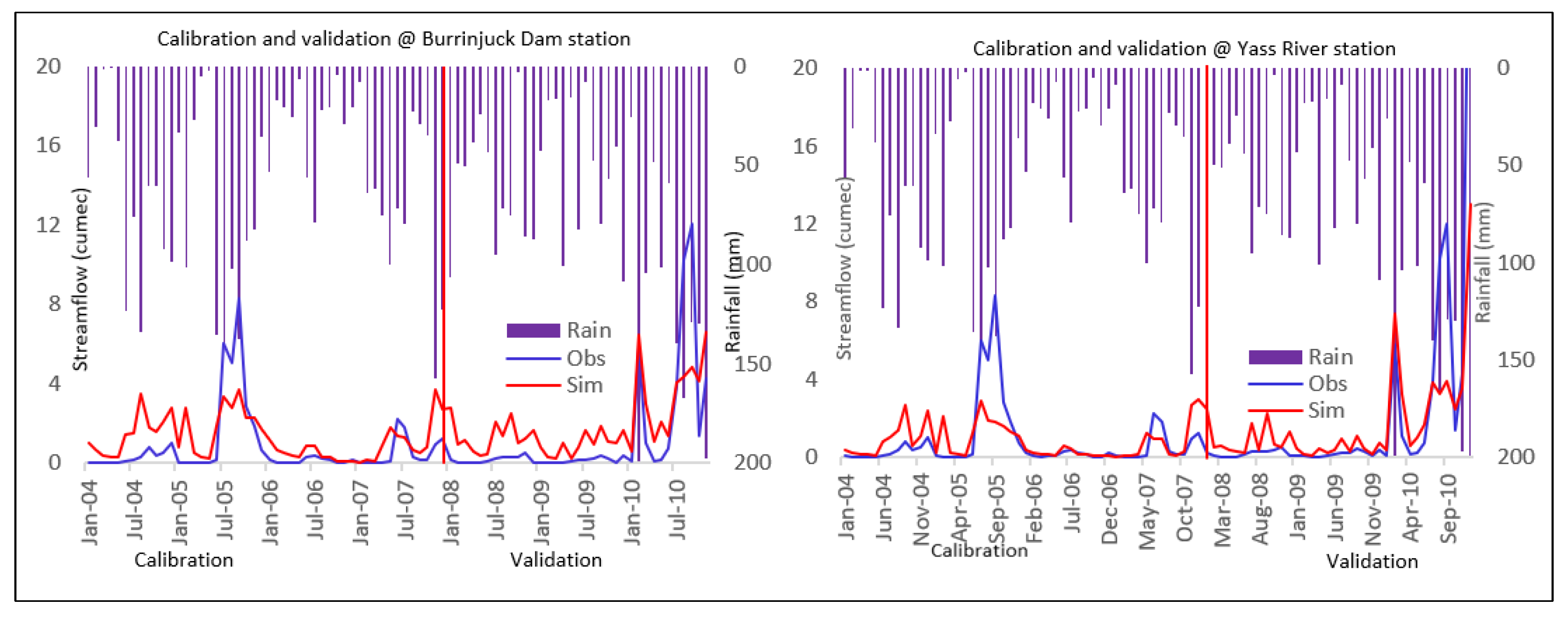
3.1. Hydrological Model Calibration and Validation
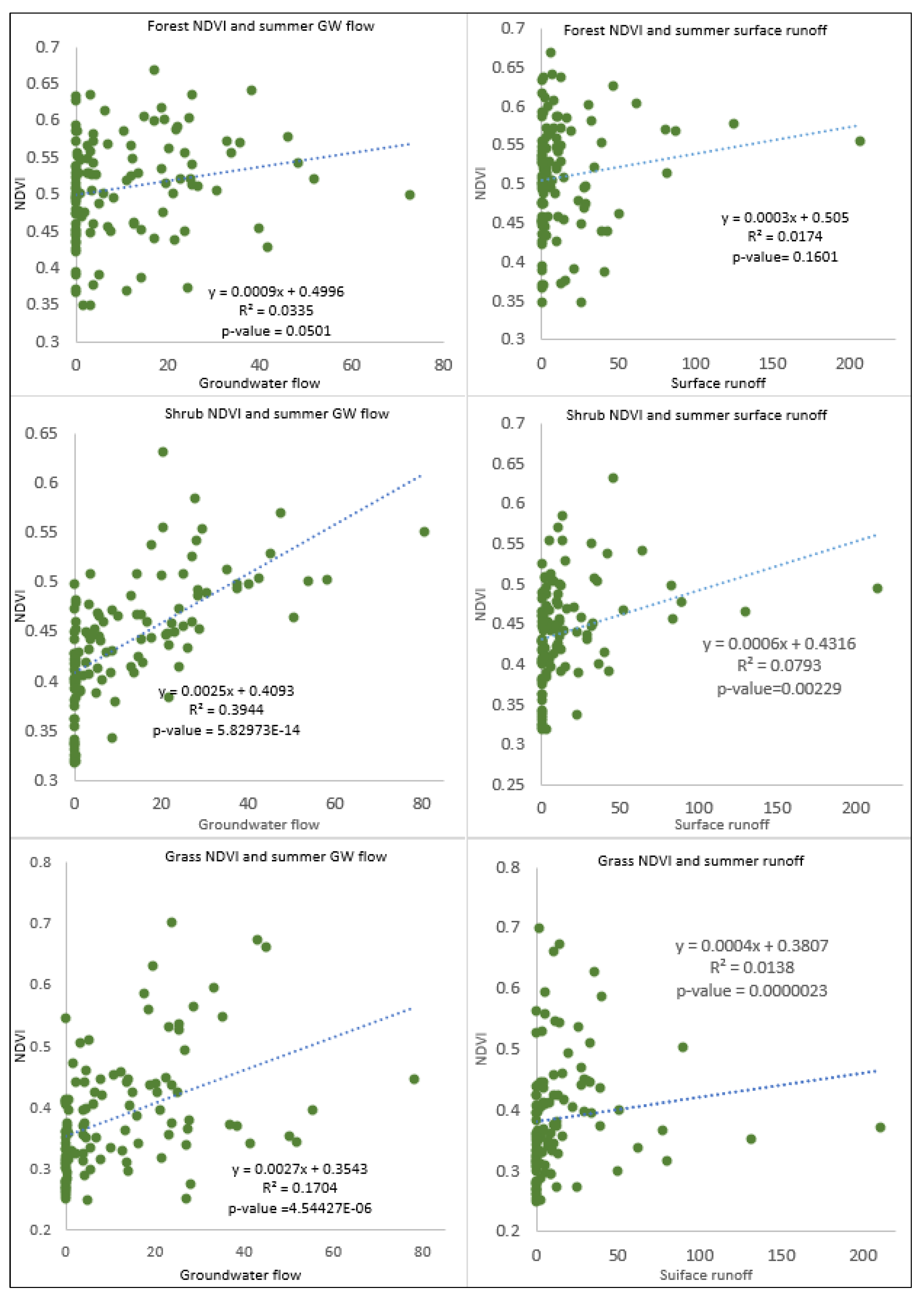
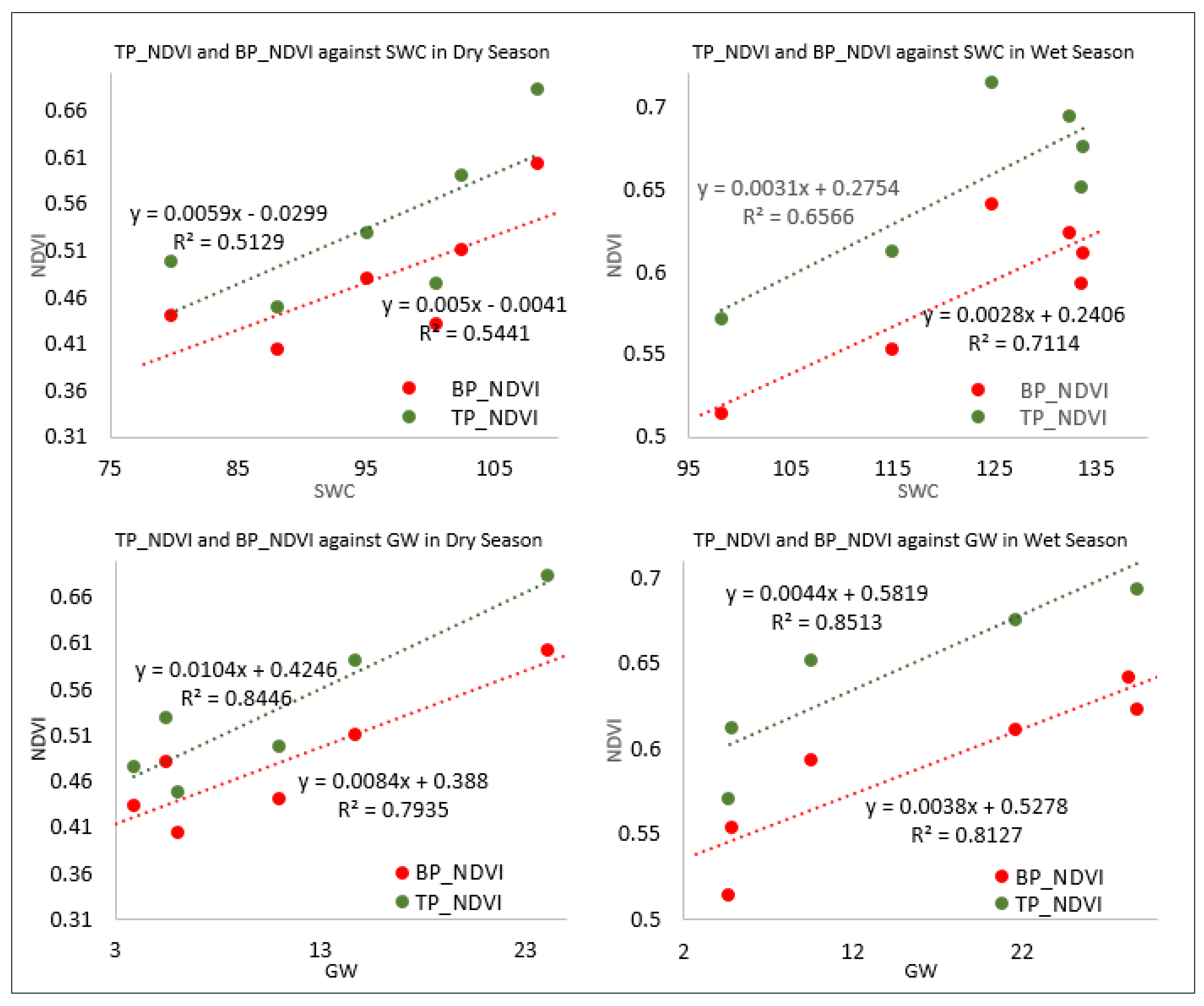
3.2. Relationships of Vegetation Responses and Groundwater
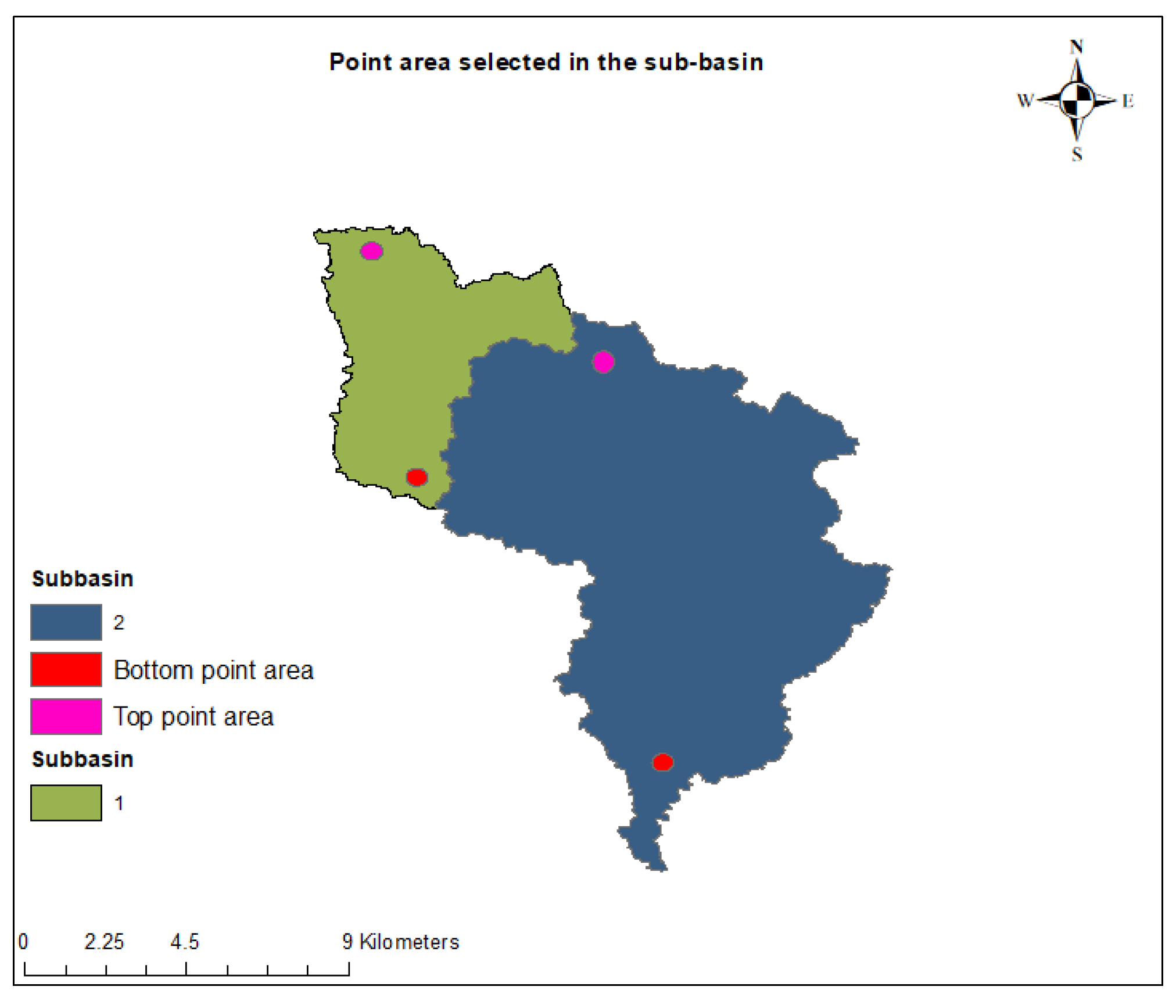
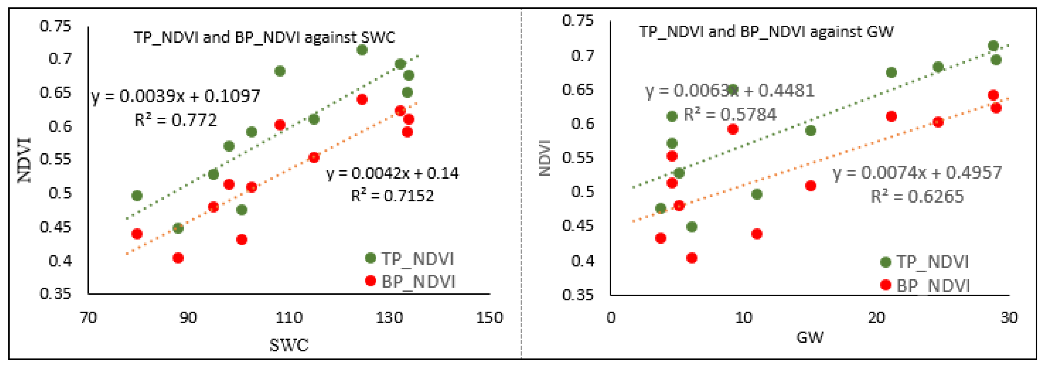
3.3. Vegetation Responses Considering Their Location within the Watershed
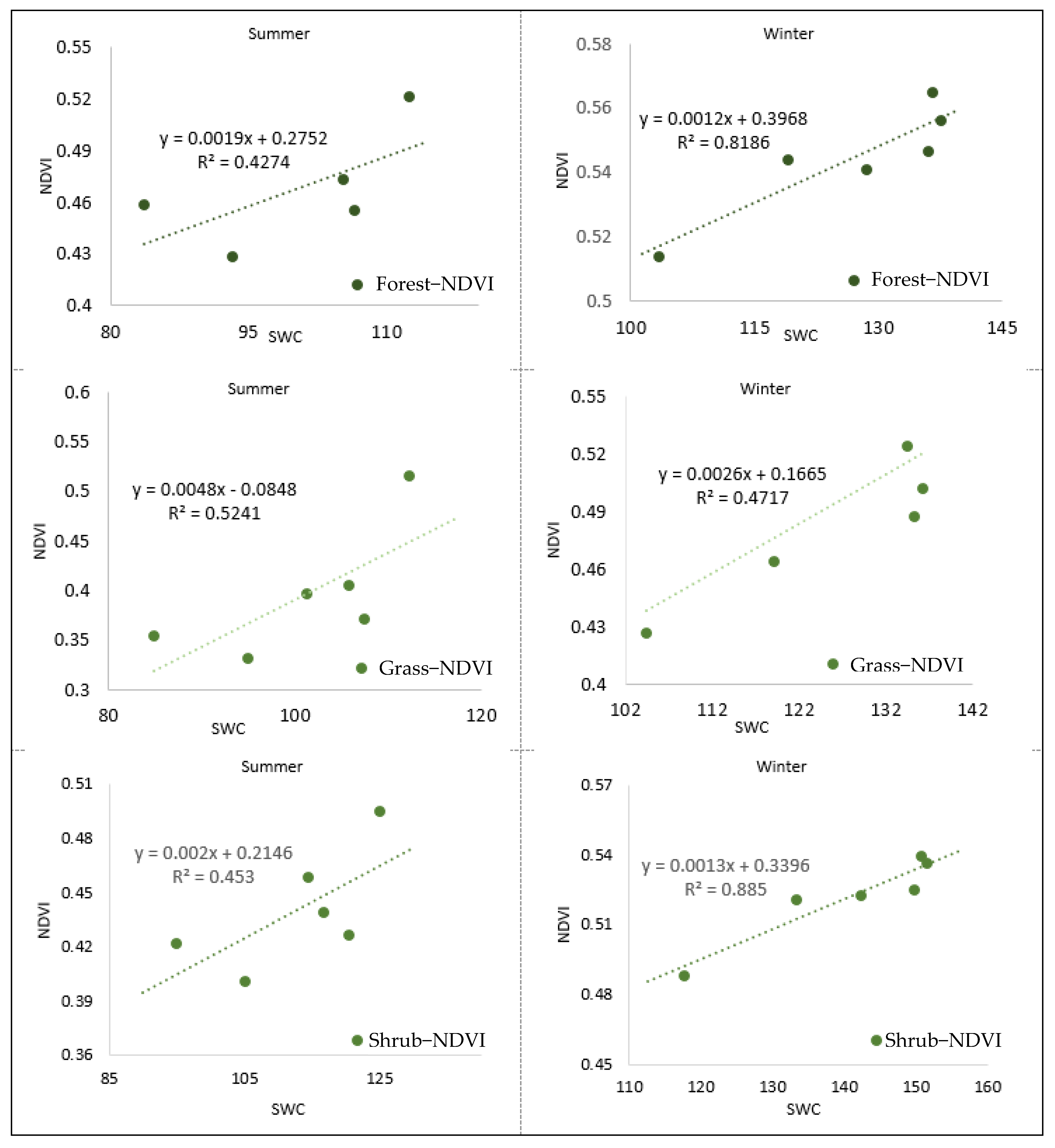
3.4. Seasonal Vegetation Responses
4. Discussion
4.1. Relationship between Vegetation Responses (NDVI) and ArcSWAT Model Simulated Soil Water Content (SWC) and Groundwater Flow (GW) Considering Vegetation Types and Their Locations
4.2. Seasonal Variability in Each Vegetation Type
5. Conclusions
Author Contributions
Funding
Data Availability Statement
Acknowledgments
Conflicts of Interest
Appendix A

References
- Ponting, J.; Kelly, T.J.; Verhoef, A.; Watts, M.J.; Sizmur, T. The impact of increased flooding occurrence on the mobility of potentially toxic elements in floodplain soil—A review. Sci. Total Environ. 2021, 754, 142040. [Google Scholar] [CrossRef] [PubMed]
- Mohammed, B.; Salah, O.; Driss, O.; Abdelghani, C. Global warming and groundwater from semi-arid areas: Essaouira region (Morocco) as an example. SN Appl. Sci. 2020, 2, 1245. [Google Scholar] [CrossRef]
- Condon, L.E.; Atchley, A.L.; Maxwell, R.M. Evapotranspiration depletes groundwater under warming over the contiguous United States. Nat. Commun. 2020, 11, 873. [Google Scholar] [CrossRef] [PubMed] [Green Version]
- Huang, F.; Zhang, D.; Chen, X. Vegetation Response to Groundwater Variation in Arid Environments: Visualization of Research Evolution, Synthesis of Response Types, and Estimation of Groundwater Threshold. Int. J. Environ Res. Public Health 2019, 16, 1849. [Google Scholar] [CrossRef] [PubMed] [Green Version]
- Cheng, Y.; Yang, W.; Zhan, H.; Jiang, Q.; Shi, M.; Wang, Y. On the Origin of Deep Soil Water Infiltration in the Arid Sandy Region of China. Water 2020, 12, 2409. [Google Scholar] [CrossRef]
- Ma, X.; Huete, A.; Moran, S.; Ponce-Campos, G.; Eamus, D. Abrupt shifts in phenology and vegetation productivity under climate extremes. J. Geophys. Res. Biogeosciences 2015, 120, 2036–2052. [Google Scholar] [CrossRef]
- Dai, A. Drought under global warming: A review. WIREs Clim. Change 2011, 2, 45–65. [Google Scholar] [CrossRef] [Green Version]
- Wang, P.; Zhang, Y.; Yu, J.; Fu, G.; Ao, F. Vegetation dynamics induced by groundwater fluctuations in the lower Heihe River Basin, northwestern China. J. Plant Ecol. 2011, 4, 77–90. [Google Scholar] [CrossRef]
- Schmugge, T.J.; Jackson, T.J.; McKim, H.L. Survey of methods for soil moisture determination. Water Resour. Res. 1980, 16, 961–979. [Google Scholar] [CrossRef] [Green Version]
- Uniyal, B.; Dietrich, J.; Vasilakos, C.; Tzoraki, O. Evaluation of SWAT simulated soil moisture at catchment scale by field measurements and Landsat derived indices. Agric. Water Manag. 2017, 193, 55–70. [Google Scholar] [CrossRef]
- Porporato, A.; Daly, E.; Rodriguez-Iturbe, I. Soil water balance and ecosystem response to climate change. Am. Nat. 2004, 164, 625–632. [Google Scholar] [CrossRef] [PubMed]
- Tian, S.; Renzullo, L.J.; van Dijk, A.I.J.M.; Tregoning, P.; Walker, J.P. Global joint assimilation of GRACE and SMOS for improved estimation of root-zone soil moisture and vegetation response. Hydrol. Earth Syst. Sci. 2019, 23, 1067–1081. [Google Scholar] [CrossRef] [Green Version]
- Leenaars, J.G.; Claessens, L.; Heuvelink, G.B.; Hengl, T.; González, M.R.; van Bussel, L.G.; Guilpart, N.; Yang, H.; Cassman, K.G. Mapping rootable depth and root zone plant-available water holding capacity of the soil of sub-Saharan Africa. Geoderma 2018, 324, 18–36. [Google Scholar] [CrossRef] [PubMed]
- Zhu, Y.; Wu, Y.; Drake, S. A survey: Obstacles and strategies for the development of ground-water resources in arid inland river basins of Western China. J. Arid. Environ. 2004, 59, 351–367. [Google Scholar] [CrossRef]
- Naumburg, E.; Mata-Gonzalez, R.; Hunter, R.G.; McLendon, T.; Martin, D.W. Phreatophytic Vegetation and Groundwater Fluctuations: A Review of Current Research and Application of Ecosystem Response Modeling with an Emphasis on Great Basin Vegetation. Environ. Manag. 2005, 35, 726–740. [Google Scholar] [CrossRef]
- Schlaepfer, D.R.; Bradford, J.B.; Lauenroth, W.K.; Munson, S.M.; Tietjen, B.; Hall, S.A.; Wilson, S.D.; Duniway, M.C.; Jia, G.; Pyke, D.A.; et al. Climate change reduces extent of temperate drylands and intensifies drought in deep soils. Nat. Commun. 2017, 8, 14196. [Google Scholar] [CrossRef] [Green Version]
- Tomlinson, M.; Boulton, A.J. Ecology and management of subsurface groundwater dependent ecosystems in Australia—A review. Mar. Freshw. Res. 2010, 61, 936–949. [Google Scholar] [CrossRef]
- Zhu, Y.; Chen, Y.; Ren, L.; Lü, H.; Zhao, W.; Yuan, F.; Xu, M. Ecosystem restoration and conservation in the arid inland river basins of Northwest China: Problems and strategies. Ecol. Eng. 2016, 94, 629–637. [Google Scholar] [CrossRef]
- Eamus, D.; Zolfaghar, S.; Villalobos-Vega, R.; Cleverly, J.; Huete, A. Groundwater-dependent ecosystems: Recent insights from satellite and field-based studies. Hydrol. Earth Syst. Sci. 2015, 19, 4229–4256. [Google Scholar] [CrossRef] [Green Version]
- Adhikari, R.K.; Mohanasundaram, S.; Shrestha, S. Impacts of land-use changes on the groundwater recharge in the Ho Chi Minh city, Vietnam. Environ Res. 2020, 185, 109–440. [Google Scholar] [CrossRef]
- Arnold, J.G.; Moriasi, D.N.; Gassman, P.W.; Abbaspour, K.C.; White, M.J.; Srinivasan, R.; Jha, M.K. SWAT: Model use, calibration, and validation. Trans. ASABE 2012, 55, 1491–1508. [Google Scholar] [CrossRef]
- Cuceloglu, G.; Abbaspour, K.C.; Ozturk, I. Assessing the Water-Resources Potential of Istanbul by Using a Soil and Water Assessment Tool (SWAT) Hydrological Model. Water 2017, 9, 814. [Google Scholar] [CrossRef] [Green Version]
- Francesconi, W.; Srinivasan, R.; Pérez-Miñana, E.; Willcock, S.P.; Quintero, M. Using the Soil and Water Assessment Tool (SWAT) to model ecosystem services: A systematic review. J. Hydrol. 2016, 535, 625–636. [Google Scholar] [CrossRef]
- Pisinaras, V.; Petalas, C.; Gikas, G.D.; Gemitzi, A.; Tsihrintzis, V.A. Hydrological and water quality modeling in a medium-sized basin using the Soil and Water Assessment Tool (SWAT). Desalination 2010, 250, 274–286. [Google Scholar] [CrossRef]
- Silva-Júnior, R.O.D.; Salomão, G.N.; Tavares, A.L.; Santos, J.F.D.; Santos, D.C.; Dias, L.C.; Rocha, E.J.P.D. Response of Water Balance Components to Changes in Soil Use and Vegetation Cover Over Three Decades in the Eastern Amazon. Front. Water 2021, 3, 1. [Google Scholar] [CrossRef]
- Yonaba, R.; Biaou, A.C.; Koïta, M.; Tazen, F.; Mounirou, L.A.; Zouré, C.O.; Queloz, P.; Karambiri, H.; Yacouba, H. A dynamic land use/land cover input helps in picturing the Sahelian paradox: Assessing variability and attribution of changes in surface runoff in a Sahelian watershed. Sci. Total Environ. 2021, 757, 143792. [Google Scholar] [CrossRef] [PubMed]
- Narasimhan, B.; Srinivasan, R. Development and evaluation of Soil Moisture Deficit Index (SMDI) and Evapotranspiration Deficit Index (ETDI) for agricultural drought monitoring. Agric. For. Meteorol. 2005, 133, 69–88. [Google Scholar] [CrossRef]
- Saha, P.; Zeleke, K. Assessment of streamflow and catchment water balance sensitivity to climate change for the Yass River catchment in south eastern Australia. Environ. Earth Sci. 2014, 73, 6229–6242. [Google Scholar] [CrossRef]
- Fu, B.; Burgher, I. Riparian vegetation NDVI dynamics and its relationship with climate, surface water and groundwater. J. Arid. Environ. 2015, 113, 59–68. [Google Scholar] [CrossRef]
- Mallick, J.; AlMesfer, M.; Singh, V.; Falqi, I.; Singh, C.; Alsubih, M.; Kahla, N. Evaluating the NDVI–Rainfall Relationship in Bisha Watershed, Saudi Arabia Using Non-Stationary Modeling Technique. Atmosphere 2021, 12, 593. [Google Scholar] [CrossRef]
- Nouri, H.; Anderson, S.; Sutton, P.; Beecham, S.; Nagler, P.; Jarchow, C.J.; Roberts, D.A. NDVI, scale invariance and the modifiable areal unit problem: An assessment of vegetation in the Adelaide Parklands. Sci. Total Environ. 2017, 584–585, 11–18. [Google Scholar] [CrossRef]
- Park, J.-Y.; Ahn, S.-R.; Hwang, S.-J.; Jang, C.-H.; Park, G.-A.; Kim, S.-J. Evaluation of MODIS NDVI and LST for indicating soil moisture of forest areas based on SWAT modeling. Paddy Water Environ. 2014, 12, 77–88. [Google Scholar] [CrossRef]
- Groeneveld, D.P.; Baugh, W.M.; Sanderson, J.S.; Cooper, D.J. Annual Groundwater Evapotranspiration Mapped from Single Satellite Scenes. J. Hydrol. 2007, 344, 146–156. [Google Scholar] [CrossRef]
- Nanzad, L.; Zhang, J.; Tuvdendorj, B.; Nabil, M.; Zhang, S.; Bai, Y. NDVI anomaly for drought monitoring and its correlation with climate factors over Mongolia from 2000 to 2016. J. Arid. Environ. 2019, 164, 69–77. [Google Scholar] [CrossRef]
- Wen, L.; Macdonald, R.; Morrison, T.; Hameed, T.; Saintilan, N.; Ling, J. From hydrodynamic to hydrological modelling: Investigating long-term hydrological regimes of key wetlands in the Macquarie Marshes, a semi-arid lowland floodplain in Australia. J. Hydrol. 2013, 500, 45–61. [Google Scholar] [CrossRef]
- Aguilar, C.; Zinnert, J.C.; Polo, M.J.; Young, D.R. NDVI as an indicator for changes in water availability to woody vegetation. Ecol. Indic. 2012, 23, 290–300. [Google Scholar] [CrossRef]
- Bhanja, S.N.; Malakar, P.; Mukherjee, A.; Rodell, M.; Mitra, P.; Sarkar, S. Using Satellite-Based Vegetation Cover as Indicator of Groundwater Storage in Natural Vegetation Areas. Geophys. Res. Lett. 2019, 46, 8082–8092. [Google Scholar] [CrossRef]
- Seeyan, S.; Merkel, B.; Abo, R. Investigation of the Relationship between Groundwater Level Fluctuation and Vegetation Cover by using NDVI for Shaqlawa Basin, Kurdistan Region—Iraq. J. Geogr. Geol. 2014, 6, 187. [Google Scholar] [CrossRef] [Green Version]
- Eibe, F.; Mark, A.H.; Ian, H.W. The WEKA Workbench. Online Appendix for “Data Mining: Practical Machine Learning Tools and Techniques”, 4th ed.; Kaufmann, M., Ed.; University of Waikato: Burlington, MA, USA, 2016. [Google Scholar]
- Hall, M.; Frank, E.; Holmes, G.; Pfahringer, B.; Reutemann, P.; Witten, I.H. The WEKA data mining software. ACM SIGKDD Explor. Newsl. 2009, 11, 10–18. [Google Scholar] [CrossRef]
- Marin, D.B.; Ferraz, G.A.E.S.; Santana, L.S.; Barbosa, B.D.S.; Barata, R.A.P.; Osco, L.P.; Ramos, A.P.M.; Guimarães, P.H.S. Detecting coffee leaf rust with UAV-based vegetation indices and decision tree machine learning models. Comput. Electron. Agric. 2021, 190, 106476. [Google Scholar] [CrossRef]
- Sharma, A.K.; Kumar, A.; Saxena, S.; Beniwal, M. Evaluating WEKA over the Open Source Web Data Mining Tools. Int. J. Eng. Res. Technol. 2015, 8, 128–132. [Google Scholar]
- Brown, A.E.; Podger, G.M.; Davidson, A.J.; Dowling, T.I.; Zhang, L. Predicting the impact of plantation forestry on water users at local and regional scales: An example for the Murrumbidgee River Basin, Australia. For. Ecol. Manag. 2007, 251, 82–93. [Google Scholar] [CrossRef]
- Saha, P.; Zeleke, K.; Hafeez, M. Streamflow modeling in a fluctuant climate using SWAT: Yass River catchment in south eastern Australia. Environ. Earth Sci. 2013, 71, 5241–5254. [Google Scholar] [CrossRef]
- Wallbrink, P.J.; Olley, J.M.; Murray, A.S. The Contribution of Subsoil to Sediment Yield in the Murrumbidgee River Basin, New South Wales, Australia; IAHS: Wallingford, UK, 1996. [Google Scholar]
- Verstraeten, G.; Prosser, I.P.; Fogarty, P. Predicting the spatial patterns of hillslope sediment delivery to river channels in the Murrumbidgee catchment, Australia. J. Hydrol. 2007, 334, 440–454. [Google Scholar] [CrossRef]
- Green, D.; Petrovic, J.; Moss, P.; Burrell, M. Water Resources and Management Overview: Murrumbidgee Catchment; NSW Office of Water: Sydney, Australia, 2011.
- Peel, M.; Finlayson, B.; McMahon, T. Updated world map of the Köpper-Geiger climate classification. Hydrol. Earth Syst. Sci. 2007, 11, 439–472. [Google Scholar] [CrossRef] [Green Version]
- Cracknell, M.J.; Reading, A.M. Geological mapping using remote sensing data: A comparison of five machine learning algorithms, their response to variations in the spatial distribution of training data and the use of explicit spatial information. Comput. Geosci. 2014, 63, 22–33. [Google Scholar] [CrossRef] [Green Version]
- ESRI. ArcGIS Deskto2019; Environmental Systems Research Institute: Redlands, CA, USA, 2019. [Google Scholar]
- Microsoft Corporation. Microsoft Excel; Corporation, M., Ed.; Microsoft Corporation: Redmond, WA, USA, 2018. [Google Scholar]
- Smith, T.C.; Frank, E. Introducing machine learning concepts with WEKA. In Statistical Genomics; Humana Press: Totowa, NJ, USA, 2016; pp. 353–378. [Google Scholar]
- Neitsch, S.L.; Arnold, J.G.; Kiniry, J.R.; Williams, J.R. SWAT Theoretical Documentation Version 2009. Texas Water Resources Institute Technical Report No. 406; Texas Water Resources Institute: College Station, TX, USA, 2011. [Google Scholar]
- Gassman, P.; Sadeghi, A.; Srinivasan, R. Applications of the SWAT Model Special Section: Overview and Insights. J. Environ. Qual. 2014, 43, 1–8. [Google Scholar] [CrossRef] [PubMed]
- USGS. Earth Explorer. US Geological Survey. Available online: https://earthexplorer.usgs.gov/ (accessed on 28 April 2022).
- Setegn, S.G.; Srinivasan, R.; Melesse, A.M.; Dargahi, B. SWAT Model Application and Prediction Uncertainty Analysis in the Lake Tana Basin, Ethiopia. Hydrol. Process. 2009, 24, 357–367. [Google Scholar] [CrossRef]
- BOM. Climate Data Online. Australian Bureau of Meteorology. Available online: http://www.bom.gov.au/climate/data/index.shtml (accessed on 19 April 2022).
- Fassò, A.; Sommer, M.; von Rohden, C. Interpolation uncertainty of atmospheric temperature profiles. Atmos. Meas. Tech. 2020, 13, 6445–6458. [Google Scholar] [CrossRef]
- de Andrade, C.W.; Montenegro, S.M.; Montenegro, A.A.; Lima JR, D.S.; Srinivasan, R.; Jones, C.A. Soil moisture and discharge modeling in a representative watershed in northeastern Brazil using SWAT. Ecohydrol. Hydrobiol. 2019, 19, 238–251. [Google Scholar] [CrossRef]
- Abbaspour, K.C.; Vaghefi, S.A.; Srinivasan, R. A Guideline for Successful Calibration and Uncertainty Analysis for Soil and Water Assessment: A Review of Papers from the 2016 International SWAT Conference. Water 2018, 10, 6. [Google Scholar] [CrossRef]
- Abbaspour, K.C.; Rouholahnejad, E.; Vaghefi, S.; Srinivasan, R.; Yang, H.; Kløve, B. A continental-scale hydrology and water quality model for Europe: Calibration and uncertainty of a high-resolution large-scale SWAT model. J. Hydrol. 2015, 524, 733–752. [Google Scholar] [CrossRef] [Green Version]
- Abbaspour, K.C.; Johnson, C.; Van Genuchten, M.T. Estimating uncertain flow and transport parameters using a sequential uncertainty fitting procedure. Vadose Zone J. 2004, 3, 1340–1352. [Google Scholar] [CrossRef]
- Moriasi, D.N.; Arnold, J.G.; van Liew, M.W.; Bingner, R.L.; Harmel, R.D.; Veith, T.L. Model Evaluation Guidelines for Systematic Quantification of Accuracy in Watershed Simulations. Trans. ASABE 2007, 50, 885–900. [Google Scholar] [CrossRef]
- Zhang, Y.; Chiew, F.H.S.; Zhang, L.; Li, H. Use of Remotely Sensed Actual Evapotranspiration to Improve Rainfall Runoff Modeling in Southeast Australia. J. Hydrometeorol. 2009, 10, 969–980. [Google Scholar] [CrossRef]
- Nash, J.E.; Sutcliffe, J.V. River flow forecasting through conceptual models part I—A discussion of principles. J. Hydrol. 1970, 10, 282–290. [Google Scholar] [CrossRef]
- Wu, L.; Liu, X.; Yang, Z.; Yu, Y.; Ma, X. Effects of single- and multi-site calibration strategies on hydrological model performance and parameter sensitivity of large-scale semi-arid and semi-humid watersheds. Hydrol. Process. 2022, 36, e14616. [Google Scholar] [CrossRef]
- EarthData. Application for Extracting and Exploring Analysis Ready Samples (AρρEEARS). 2021. Available online: https://appeears.earthdatacloud.nasa.gov/ (accessed on 26 April 2022).
- Sarkar, A. Deep Learning and the Evolution of Useful Information. Inf. Matters 2021, 1, 6. [Google Scholar] [CrossRef]
- Jiao, L.; An, W.; Li, Z.; Gao, G.; Wang, C. Regional variation in soil water and vegetation characteristics in the Chinese Loess Plateau. Ecol. Indic. 2020, 115, 106399. [Google Scholar] [CrossRef]
- He, B.; Chen, A.; Jiang, W.; Chen, Z. The response of vegetation growth to shifts in trend of temperature in China. J. Geogr. Sci. 2017, 27, 801–816. [Google Scholar] [CrossRef] [Green Version]
- Sheykhmousa, M.; Mahdianpari, M.; Ghanbari, H.; Mohammadimanesh, F.; Ghamisi, P.; Homayouni, S. Support Vector Machine Versus Random Forest for Remote Sensing Image Classification: A Meta-Analysis and Systematic Review. IEEE J. Sel. Top. Appl. Earth Obs. Remote Sens. 2020, 13, 6308–6325. [Google Scholar] [CrossRef]
- Sandi, S.G.; Rodriguez, J.F.; Saintilan, N.; Wen, L.; Kuczera, G.; Riccardi, G.; Saco, P.M. Resilience to drought of dryland wetlands threatened by climate change. Sci. Rep. 2020, 10, 13232. [Google Scholar] [CrossRef] [PubMed]


| Data | Frequency | Description | Source |
|---|---|---|---|
| Precipitation | Daily | Station gauged, temporal | Bureau of Meteorology |
| Temperature | Daily | Station gauged, temporal | Bureau of Meteorology |
| Evapotranspiration Wind speed | Daily Hourly | Satellite-derived, 0.05 degree (approximately 5 × 5 km) Station gauged, temporal | Bureau of Meteorology Bureau of Meteorology |
| Runoff | Daily | Satellite-derived, 0.05 degree (approximately 5 × 5 km) | Bureau of Meteorology |
| Streamflow (discharge) | Daily | Station gauged, temporal | NSW Office of Water |
| MODIS NDVI | 16-Day | 250 m spatial resolution | U.S. Geological Survey |
| DEM | - | 30 m spatial resolution | U.S. Geological Survey |
| Soil Map | - | 250 m spatial resolution | Digital Atlas of Australian Soil |
| Land cover/land use map | - | 50 m spatial resolution | NSW Office of Environment and Heritage |
| Parameter Definition | Value Range | Unit | Method | Par.inputfile | Ranking |
|---|---|---|---|---|---|
| Initial SCS runoff curve number for moisture condition | 35–89 | % | r | CN2 | 1 |
| Effective hydraulic conductivity in the main channel alluvium | 0–500 | mm/h | v | CH_K2.rte | 13 |
| Manning’s n value for the main channel | 0–0.3 | — | v | CH_N2.rte | 12 |
| Base flow alpha factor | 0–1 | days | v | ALPHA_BF.gw | 5 |
| Groundwater delay | 30–500 | days | v | GW_DELAY.gw | 10 |
| Groundwater “revap” coefficient | 0.02–0.2 | — | v | GW_REVAP.gw | 11 |
| Threshold depth of water in the shallow aquifer for return flow to occur | 0–5000 | mm H2O | v | GWQMN.gw | 3 |
| Threshold depth of water in the shallow aquifer required for “revap” to occur | 0–1 | mm H2O | v | REVAPMN.gw | 8 |
| Soil evaporation compensation factor | 0–0.65 | - | v | ESCO.bsn | 2 |
| Average slope length | 10–150 | m | r | SLSUBBSN.hru | 9 |
| Surface runoff lag coefficient | 0.05–24 | — | v | SURLAG.bsn | 15 |
| Available water capacity of the soil layer | −0.5–0.5 | mmH2O/mm | r | SOL_AWC.sol | 4 |
| Depth from the soil surface to layer bottom | −0.5–0.5 | mm | r | SOL_Z.sol | 6 |
| Peak rate adjustment factor for sediment routing | 1–2 | - | r | ADJ_PKR.bsn | 14 |
| Maximum canopy storage | 0–100 | mm H2O | v | CANMX.hru | 7 |
| Scenario | NSE | R2 | PBIAS |
|---|---|---|---|
| Default | 0.25 | 0.36 | 73.2 |
| Manual calibration | 0.51 | 0.72 | 54.2 |
| SUFI-2 | 0.41 | 0.55 | 68.2 |
| Variable | January | February | March | April | May | June | July | August | September | October | November | December |
|---|---|---|---|---|---|---|---|---|---|---|---|---|
| SWC | 86.28 | 98.54 | 93.18 | 96.25 | 112.64 | 130.79 | 131.11 | 129.71 | 122.23 | 106.23 | 100.48 | 78.14 |
| GW | 6.07 | 3.72 | 5.10 | 4.59 | 4.60 | 9.13 | 21.15 | 29.00 | 28.73 | 24.57 | 15.01 | 10.96 |
| Sub-Basin | GW | SWC | SWC and GW | |||||||
|---|---|---|---|---|---|---|---|---|---|---|
| # 28 | r | RMSE | RRSE | r | RMSE | RRSE | r | RMSE | RRSE | |
| FOREST | SVM | 0.373 | 0.064 | 91% | 0.592 | 0.055 | 79% | 0.610 | 0.055 | 78% |
| RF | 0.219 | 0.076 | 110.42% | 0.446 | 0.067 | 91% | 0.540 | 0.060 | 85% | |
| SB_NDVI | SVM | 0.597 | 0.075 | 80% | 0.710 | 0.066 | 70% | 0.781 | 0.059 | 62% |
| RF | 0.484 | 0.088 | 94% | 0.604 | 0.079 | 84% | 0.736 | 0.064 | 68% | |
| TP_NDVI | SVM | 0.471 | 0.072 | 89% | 0.624 | 0.063 | 78% | 0.660 | 0.061 | 75% |
| RF | 0.407 | 0.080 | 98% | 0.624 | 0.063 | 78% | 0.631 | 0.064 | 79% | |
| BP_NDVI | SVM | 0.267 | 0.072 | 96% | 0.513 | 0.064 | 85% | 0.521 | 0.063 | 85% |
| RF | 0.132 | 0.085 | 113% | 0.330 | 0.078 | 104% | 0.434 | 0.070 | 93% | |
| Sub-Basin | GW | SWC | SWC and GW | |||||||
|---|---|---|---|---|---|---|---|---|---|---|
| # 19 | r | RMSE | RRSE | r | RMSE | RRSE | r | RMSE | RRSE | |
| SHRUB | SVM | 0.533 | 0.059 | 82% | 0.681 | 0.051 | 70% | 0.671 | 0.052 | 72% |
| RF | 0.596 | 0.056 | 77.96% | 0.625 | 0.055 | 74% | 0.626 | 0.054 | 74% | |
| SB_NDVI | SVM | 0.579 | 0.073 | 82% | 0.689 | 0.064 | 72% | 0.759 | 0.058 | 65% |
| RF | 0.462 | 0.084 | 94% | 0.577 | 0.076 | 85% | 0.685 | 0.066 | 74% | |
| TP_NDVI | SVM | 0.674 | 0.078 | 74% | 0.697 | 0.075 | 71% | 0.812 | 0.061 | 58% |
| RF | 0.609 | 0.087 | 82% | 0.571 | 0.090 | 86% | 0.772 | 0.067 | 64% | |
| BP_NDVI | SVM | 0.247 | 0.082 | 97% | 0.456 | 0.075 | 89% | 0.451 | 0.075 | 89% |
| RF | 0.041 | 0.098 | 117% | 0.267 | 0.091 | 108% | 0.363 | 0.082 | 97% | |
| Sub-Basin | GW | SWC | SWC and GW | |||||||
|---|---|---|---|---|---|---|---|---|---|---|
| # 23 | r | RMSE | RRSE | r | RMSE | RRSE | r | RMSE | RRSE | |
| GRASS | SVM | 0.4642 | 0.1116 | 84.57% | 0.5342 | 0.105 | 79.28% | 0.5629 | 0.1024 | 76.98% |
| RF | 0.4876 | 0.1094 | 83.15% | 0.4607 | 0.112 | 82.75% | 0.4955 | 0.1088 | 80.10% | |
| SB_NDVI | SVM | 0.6004 | 0.1071 | 80.63% | 0.649 | 0.1007 | 75.75% | 0.7431 | 0.0889 | 66.92% |
| RF | 0.5369 | 0.1171 | 88.10% | 0.4353 | 0.1299 | 97.78% | 0.6522 | 0.1025 | 77.11% | |
| TP_NDVI | SVM | 0.6528 | 0.1276 | 75.90% | 0.6729 | 0.1238 | 73.62% | 0.7883 | 0.1035 | 61.55% |
| RF | 0.581 | 0.1422 | 84.62% | 0.4665 | 0.1605 | 95.47% | 0.7031 | 0.121 | 71.97% | |
| BP_NDVI | SVM | −0.0069 | 0.1265 | 101.07% | 0.1134 | 0.1242 | 99.19% | 0.2045 | 0.1223 | 97.67% |
| RF | −0.0646 | 0.1519 | 121.35% | 0.0884 | 0.1438 | 114.89% | 0.1552 | 0.1312 | 104.79% | |
| Sub-basin | GW | SWC | SWC and GW | |||||||
| # 28 | r | RMSE | RRSE | r | RMSE | RRSE | r | RMSE | RRSE | |
| FOREST | SVM | 0.527 | 0.053 | 0.837 | 0.481 | 0.056 | 0.871 | 0.594 | 0.051 | 0.792 |
| RF | 0.581 | 0.053 | 0.828 | 0.317 | 0.068 | 1.074 | 0.560 | 0.054 | 0.844 | |
| SB_NDVI | SVM | 0.730 | 0.058 | 0.674 | 0.570 | 0.071 | 0.815 | 0.782 | 0.054 | 0.625 |
| RF | 0.702 | 0.062 | 0.716 | 0.434 | 0.084 | 0.974 | 0.750 | 0.058 | 0.666 | |
| TP_NDVI | SVM | 0.564 | 0.068 | 0.817 | 0.539 | 0.070 | 0.840 | 0.649 | 0.063 | 0.753 |
| RF | 0.592 | 0.069 | 0.826 | 0.379 | 0.085 | 1.017 | 0.637 | 0.065 | 0.777 | |
| BP_NDVI | SVM | 0.362 | 0.061 | 0.921 | 0.368 | 0.061 | 0.917 | 0.403 | 0.060 | 0.901 |
| RF | 0.420 | 0.063 | 0.944 | 0.254 | 0.073 | 1.099 | 0.403 | 0.062 | 0.935 | |
| Sub-basin | GW | SWC | SWC and GW | |||||||
| # 19 | r | RMSE | RRSE | r | RMSE | RRSE | r | RMSE | RRSE | |
| SHRUB | SVM | 0.629 | 0.048 | 0.777 | 0.631 | 0.048 | 0.799 | 0.666 | 0.046 | 0.766 |
| RF | 0.627 | 0.048 | .76.60% | 0.604 | 0.050 | 0.784 | 0.633 | 0.048 | 0.771 | |
| SB_NDVI | SVM | 0.755 | 0.052 | 0.650 | 0.731 | 0.054 | 0.676 | 0.812 | 0.046 | 0.580 |
| RF | 0.736 | 0.054 | 0.671 | 0.744 | 0.053 | 0.660 | 0.763 | 0.510 | 0.636 | |
| TP_NDVI | SVM | 0.780 | 0.060 | 0.594 | 0.697 | 0.075 | 0.713 | 0.729 | 0.066 | 0.687 |
| RF | 0.777 | 0.060 | 0.623 | 0.789 | 0.059 | 0.605 | 0.789 | 0.059 | 0.605 | |
| BP_NDVI | SVM | 0.424 | 0.062 | 0.892 | 0.322 | 0.065 | 0.958 | 0.442 | 0.061 | 0.893 |
| RF | 0.184 | 0.071 | 1.070 | 0.269 | 0.068 | 1.023 | 0.254 | 0.068 | 1.031 | |
| Sub-basin | GW | SWC | SWC and GW | |||||||
| # 23 | r | RMSE | RRSE | r | RMSE | RRSE | r | RMSE | RRSE | |
| GRASS | SVM | 0.271 | 0.094 | 0.967 | 0.382 | 0.090 | 0.920 | 0.412 | 0.088 | 0.902 |
| RF | 0.301 | 0.100 | 1.023 | 0.212 | 0.108 | 1.115 | 0.473 | 0.087 | 0.897 | |
| SB_NDVI | SVM | 0.696 | 0.088 | 0.728 | 0.571 | 0.098 | 0.811 | 0.756 | 0.078 | 0.648 |
| RF | 0.572 | 0.101 | 0.837 | 0.442 | 0.116 | 0.956 | 0.730 | 0.083 | 0.682 | |
| TP_NDVI | SVM | 0.708 | 0.109 | 0.709 | 0.575 | 0.124 | 0.808 | 0.763 | 0.100 | 0.649 |
| RF | 0.553 | 0.133 | 0.860 | 0.503 | 0.140 | 0.907 | 0.737 | 0.103 | 0.671 | |
| BP_NDVI | SVM | −0.128 | 0.116 | 1.025 | −0.206 | 0.116 | 1.026 | 0.008 | 0.123 | 1.092 |
| RF | −0.111 | 0.138 | 1.225 | −0.139 | 0.138 | 1.227 | −0.202 | 0.118 | 1.043 | |
| Sub-basin | GW | SWC | SWC and GW | |||||||
| # 28 | r | RMSE | RRSE | r | RMSE | RRSE | r | RMSE | RRSE | |
| FOREST | SVM | 0.163 | 0.050 | 98% | 0.372 | 0.047 | 93% | 0.356 | 0.048 | 0.934 |
| RF | 0.230 | 0.055 | 107% | 0.182 | 0.058 | 114% | 0.242 | 0.053 | 1.035 | |
| SB_NDVI | SVM | 0.501 | 0.060 | 86% | 0.623 | 0.054 | 78% | 0.710 | 0.049 | 0.699 |
| RF | 0.530 | 0.066 | 94% | 0.458 | 0.067 | 96% | 0.640 | 0.055 | 0.785 | |
| TP_NDVI | SVM | 0.246 | 0.057 | 96% | 0.371 | 0.054 | 92% | 0.358 | 0.055 | 0.927 |
| RF | 0.361 | 0.058 | 99% | 0.060 | 0.071 | 121% | 0.092 | 0.076 | 1.288 | |
| BP_NDVI | SVM | 0.089 | 0.058 | 99% | 0.245 | 0.057 | 97% | 0.203 | 0.057 | 0.981 |
| RF | 0.159 | 0.063 | 108% | 0.028 | 0.071 | 121% | 0.048 | 0.066 | 1.120 | |
| Sub-basin | GW | SWC | SWC and GW | |||||||
| # 19 | r | RMSE | RRSE | r | RMSE | RRSE | r | RMSE | RRSE | |
| SHRUB | SVM | 0.346 | 0.045 | 93% | 0.431 | 0.044 | 90% | 0.445 | 0.043 | 0.892 |
| RF | 0.460 | 0.044 | 90.10% | 0.501 | 0.042 | 87% | 0.474 | 0.043 | 0.889 | |
| SB_NDVI | SVM | 0.478 | 0.062 | 87% | 0.630 | 0.055 | 77% | 0.623 | 0.056 | 0.778 |
| RF | 0.568 | 0.060 | 84% | 0.637 | 0.055 | 77% | 0.629 | 0.055 | 0.779 | |
| TP_NDVI | SVM | 0.612 | 0.072 | 79% | 0.612 | 0.072 | 79% | 0.749 | 0.060 | 0.658 |
| RF | 0.640 | 0.072 | 79% | 0.578 | 0.078 | 85% | 0.676 | 0.068 | 0.746 | |
| BP_NDVI | SVM | −0.037 | 0.076 | 101% | 0.173 | 0.075 | 99% | 0.114 | 0.076 | 1.013 |
| RF | −0.002 | 0.087 | 116% | 0.118 | 0.086 | 114% | 0.142 | 0.079 | 1.052 | |
| Sub-basin | GW | SWC | SWC and GW | |||||||
| # 23 | r | RMSE | RRSE | r | RMSE | RRSE | r | RMSE | RRSE | |
| GRASS | SVM | 0.228 | 0.120 | 97% | 0.350 | 0.117 | 94% | 0.339 | 0.117 | 0.946 |
| RF | 0.159 | 0.138 | 111% | 0.071 | 0.145 | 117% | 0.063 | 0.138 | 1.117 | |
| SB_NDVI | SVM | 0.470 | 0.102 | 88% | 0.519 | 0.099 | 85% | 0.601 | 0.092 | 0.795 |
| RF | 0.460 | 0.109 | 94% | 0.337 | 0.119 | 102% | 0.510 | 0.103 | 0.885 | |
| TP_NDVI | SVM | 0.621 | 0.109 | 78% | 0.567 | 0.115 | 82% | 0.709 | 0.098 | 0.701 |
| RF | 0.608 | 0.116 | 83% | 0.353 | 0.142 | 102% | 0.627 | 0.111 | 0.795 | |
| BP_NDVI | SVM | 0.197 | 0.115 | 98% | −0.281 | 0.117 | 100% | 0.173 | 0.117 | 0.995 |
| RF | −0.062 | 0.144 | 123% | −0.174 | 0.148 | 126% | −0.043 | 0.134 | 1.143 | |
Publisher’s Note: MDPI stays neutral with regard to jurisdictional claims in published maps and institutional affiliations. |
© 2022 by the authors. Licensee MDPI, Basel, Switzerland. This article is an open access article distributed under the terms and conditions of the Creative Commons Attribution (CC BY) license (https://creativecommons.org/licenses/by/4.0/).
Share and Cite
Muhury, N.; Apan, A.A.; Marasani, T.N.; Ayele, G.T. Modelling Floodplain Vegetation Response to Groundwater Variability Using the ArcSWAT Hydrological Model, MODIS NDVI Data, and Machine Learning. Land 2022, 11, 2154. https://doi.org/10.3390/land11122154
Muhury N, Apan AA, Marasani TN, Ayele GT. Modelling Floodplain Vegetation Response to Groundwater Variability Using the ArcSWAT Hydrological Model, MODIS NDVI Data, and Machine Learning. Land. 2022; 11(12):2154. https://doi.org/10.3390/land11122154
Chicago/Turabian StyleMuhury, Newton, Armando A. Apan, Tek N. Marasani, and Gebiaw T. Ayele. 2022. "Modelling Floodplain Vegetation Response to Groundwater Variability Using the ArcSWAT Hydrological Model, MODIS NDVI Data, and Machine Learning" Land 11, no. 12: 2154. https://doi.org/10.3390/land11122154