Who and Where Are the Observers behind Biodiversity Citizen Science Data? Effect of Landscape Naturalness on the Spatial Distribution of French Birdwatching Records

Abstract

The study of spatial bias in opportunistic data produced by citizen science programs is mainly approached either from a geographical angle (site proximity, accessibility, habitat quality) or from the angle of human behavior and volunteer engagement. In this study we linked both by analyzing the effect of observer profile on spatial distribution of recordings. We hypothesized that observer profile biases spatial distribution of records and that this bias can be explained by landscape naturalness. First, we established observer profiles from analysis of the temporal and spatial distributions of their records as well as record contents. Second, we mapped a naturalness gradient at regional and local scales. Using a dataset of more than 7 million bird records covering a time span of 15 years from the west of France, we defined four types of observer: garden-watchers, beginners, naturalists, and experts. We found that recording intensity could be related to naturalness at regional level; most visited areas were those where naturalness was on average lower i.e., close to population basins and highly accessible due to well-developed road infrastructure. At local level (neighborhood of recording sites), we found that experts and naturalists recorded in areas of higher naturalness index than those of garden-watchers and beginners. These results highlight how records contributed by different types of observer may lead to complementary coverage of different areas of the landscape. Future studies should therefore fully consider observer heterogeneity and how different observer profiles are influenced by local landscape naturalness.

1. Introduction

Citizen science—the involvement of volunteers in data collection, analysis, and interpretation—holds great promise for nature conservation [1]. Species observation data collected through citizen science allows large-scale monitoring (spatial and temporal) that would be impossible or too expensive to carry out with only professional scientists [2,3,4]. Citizen science (CS) has already made enormous contributions to conservation science, and this approach of harnessing the power of data, information and voluntary skills has the potential to do much more [5]. For a review of studies which directly contribute to understanding of the role of CS in conservation sciences, see [6].

Citizen sciences cover a large range of programs with a great diversity of methodological approaches. This diversity ranges from CS programs with standardized protocols intended for volunteers with good naturalist skills, to CS programs open to any observer which promote the collection of opportunistic data [2,7,8].

Mass participation approaches, though a powerful means of raising awareness and educating about nature and its conservation [9,10], are most often associated with unstructured monitoring programs because data collection is more flexible. In addition to the many CS-related biases, the so-called “opportunistic” data that come from these unstructured programs are more susceptible to observer bias [11]. It is well-known that researchers must exercise caution in the use of such data for modeling distributions [12] and making predictions [13].

These biases are often classified into three categories: spatial, temporal, and species-related [14,15]. It is now well-known that species presence data derived from opportunistic programs exhibit strong temporal and spatial bias. Data are not collected randomly either in time [16,17,18] or in space [19,20] leading to unfortunate gaps and redundancies. In addition, although there have been substantial improvements [21,22] these biases also include observer errors and species detectability problems due to skill heterogeneity of volunteers [23].

Among these biases, the study of spatial heterogeneity in recording intensity has a literature which can be classified into two relatively permeable categories: the first group studies that attempt to explain this heterogeneity from a geographical perspective, using landscape spatial variables; the second concerns studies that aim to explain it from a social and human perspective, using human behavior and observer engagement variables.

The first category of studies have shown that at least three landscape spatial variables can explain spatial heterogeneity in recording intensity. The first is the proximity of the “home base” [24], of “previous records” [25], of “large cities” [15,26], or of high “population density” areas [19,27]. The second is site accessibility or remoteness. It has been shown that records are more numerous in easily accessible areas [28], such as along highways [26] or in areas close to roads [19,27], than in areas remote from roads. Finally, the third often cited variable is the natural quality of the landscape. Protected areas [25], high quality habitats [12] or areas with high species richness [24,28], threatened species and habitats [25] or particular taxonomic groups [29] are more visited by observers. However, in these studies, all participants are considered to be equivalent, and no allowance is made for differences between observers.

Conversely, the other studies have sought to document the heterogeneity of participants in biodiversity CS, from social and human behavior viewpoints. The first source of participant heterogeneity noted is the type of CS program. During the past decade, CS programs have changed and diversified significantly [2] and this has been accompanied by a notable change in participation due in part to the development of Internet tools which have led to massive recruitment [30,31]. The second source of participant heterogeneity, observed within individual CS programs, is the increase in non-specialist or beginner participants from the wider general public as opposed to naturalists with expert knowledge. Seen as providing valuable insights into observers’ recording behavior, this heterogeneity has been studied in particular from the angles of motivation, temporal behavior (also called “participant engagement”) [28,32,33,34], and spatial behavior. For example, with a “behavioral ecology approach”, ref. [29] showed that local and tourist participants have different spatial recording habits. Spatial variables have also been used either to group participants (based on their spatial practices in addition to their temporal practices) [7] or in very rare studies (one to our knowledge) to link peoples’ profiles (e.g., “Dabbler”, “Steady”, “Enthusiast”) to the spatial distribution of records [28]. In the latter study, the authors showed that datasets from each of the three different programs had its own spatial and taxonomic signature depending on volunteer profile. They also found hotspots of recording intensity in sites containing open water.

A better understanding of these links could be used to better manage data biases in studies that use CS data in conservation, for example, by filtering certain groups of volunteers to obtain better spatial representativeness, as well as to reduce spatial bias by improving recommendations to participants, for example, by asking volunteers to give preference to recordings in sites that are unfamiliar to them or less attractive.

Our hypothesis was that differing observer profiles introduce spatial bias into bird recording, which can be related to landscape naturalness. Using an opportunistic bird observation dataset that includes more than 7 million data, collected over 15 years, by a wide and diverse range of people and covering an area of 32,000 km², we:

• Analyzed individual participants’ habits to identify observer profiles;
• Used the landscape naturalness gradient approach to explain the spatial distribution of observations at regional level;
• Explored the links between observer profiles and landscape naturalness in the neighborhood of their records.

2. Materials and Methods

2.1. Bird Dataset and Preprocessing

The CS bird dataset used in this study was collected by the French BirdLife International Partner (Ligue pour la Protection des Oiseaux, LPO). The data were considered as opportunistic because most came from participants who recorded whatever, wherever, and whenever they chose. Participants could contribute their records online after their outing or, since 2017, directly in the field using the smartphone application NaturaList to geolocate record. Observations may involve heard birdsongs or direct, visual observations. There is no minimum or maximum outing duration and observers are free to declare all or part of their observations. Moreover, observers do not need any prerequisites to register and they do not receive any training. The only obligation is to create an online account by specifying some mandatory personal information (e.g., identity, date of birth, address, contact number). After record declaration, a data validation procedure by a member of LPO is used to control and filter out unlikely records, which means that each record submitted must be validated to be added to the database. The dataset used in this study included more than 7 million records collected by nearly 10,000 participants. It covered a time span of 15 years (from 2005 to 2019) and a spatial extent of 32,000 km², corresponding to the administrative region of Pays-de-la-Loire in western France.

The data were prepared as follows: first, data collected and managed by several local groups were aggregated so that each record was associated with a single observer identity. Second, the aggregated dataset was checked so as to include only those records for which the observed species, date and time, X, Y coordinates, as well as observer information were available. Finally, the unified database was cleaned of incomplete and erroneous records.

2.2. Observer Profiles

Our aim was to define observer profiles based on an original set of metrics integrating spatial, temporal, and content characteristics of recording. Since the dataset used covered a period of 15 years, during which the objectives, methods and data collection tools had greatly evolved, it was assumed that observer profiles had also evolved over time leading to a certain heterogeneity in recording behavior [35]. 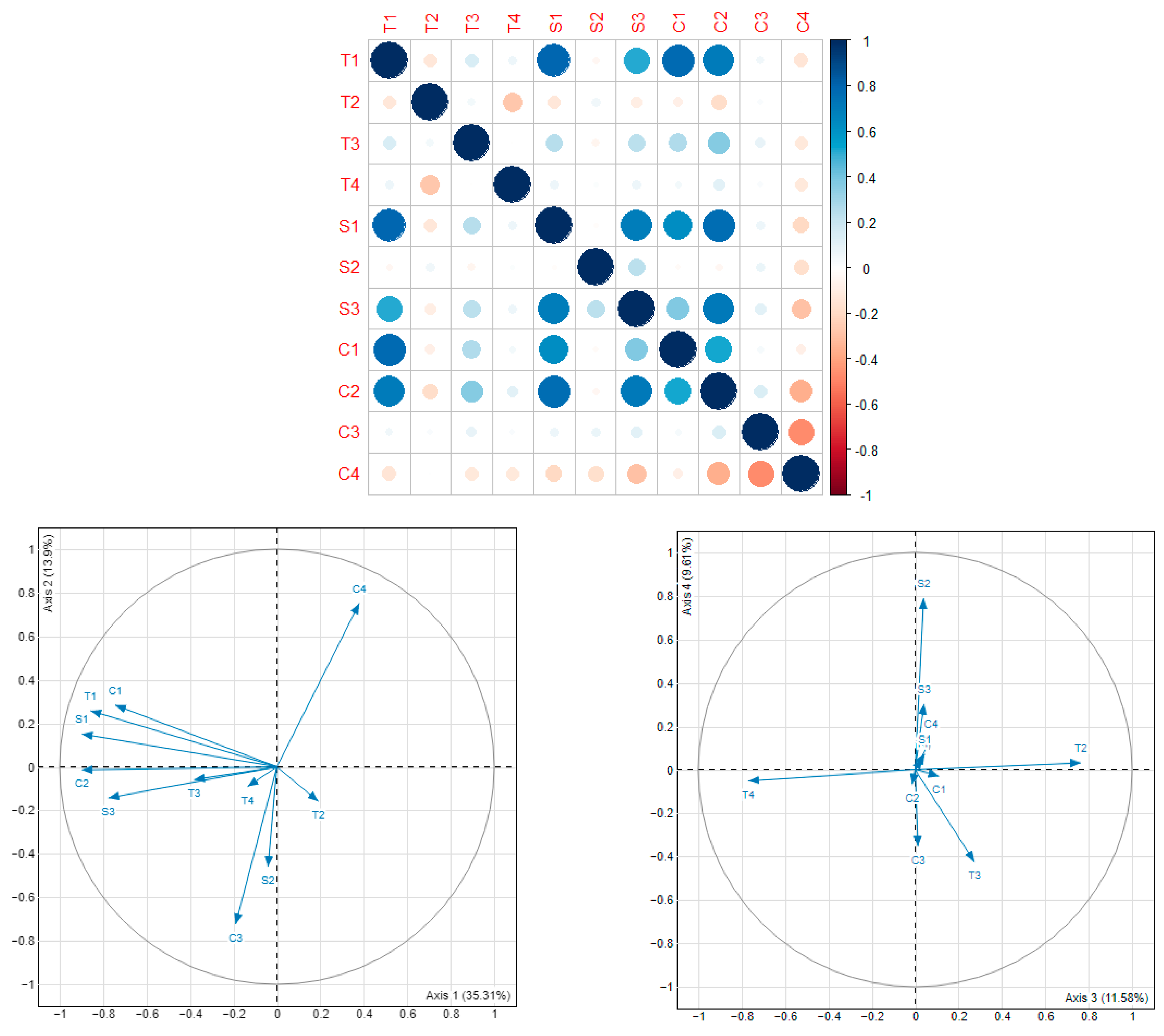We used the analysis of bird records to deduce observer habits using metrics inspired by previous work on “engagement characteristics” of participants in CS [7,28,33,34]. Initially 22 metrics were developed, of which 11 were retained after exploratory analyses, principal components analysis (PCA), and correlation tests. The table of the 22 metrics, the correlation matrix, and the PCA plots on axes 1–2 and 3–4 of the 11 metrics are given for information in Appendix A. These metrics provided information on three aspects of observer behavior: temporal habits (T) (cumulative number of recording days, recording day frequency, recording effort, percentage of records made during the week (Monday to Friday)), spatial habits (S) (spatial amplitude, spatial density, minimum geometric extent), and record quality (C) (number of records, species richness, Species Generalization Index (SGI), Species Synanthropy Index (SSI)) (

Table 1. The 11 metrics used to analyze observer profiles, in three categories (temporal habits (T), spatial habits (S), and record quality (C)), with their description and methods used for their calculation.

Metric Code	Metric Full Name	Description and Calculation Method
T1	Total number of recording days	Total number of days with at least one record from the observer
T2	Recording day frequency	Number of days between the date of registration and the date of the last record of an observer/T1
T3	Recording effort	Number of records made by an observer (C1)/T1
T4	Percentage of records made during the week	Number of records made from Monday to Friday × 100/T1
S1	Spatial amplitude	Number of 4 km2 cells in which an observer made at least one record.
S2	Spatial density	Number of records made by an observer (C1)/Area of the convex envelope of all the records of that observer (S3)
S3	Minimum geometric extent	Area of the minimum geometric extent that encompasses all the records from one observer
C1	Number of records	Total number of records made by an observer
C2	Species richness	Total number of species recorded by an observer
C3	Mean Species Generalization Index (SGI)	Mean Species Generalization Index (Godet et al., 2015) of a single observer’s records. The higher the SGI, the more generalist a species’ habitat affinity, independent of its range and local abundance
C4	Mean Species Synanthropy index (SSI)	Mean Species Synanthropy Index (Guetté et al., 2017) of a single observer’s records. The higher the SSI, the more urban “dweller” the species. The lower the SSI, the more urban “avoider” the species

).

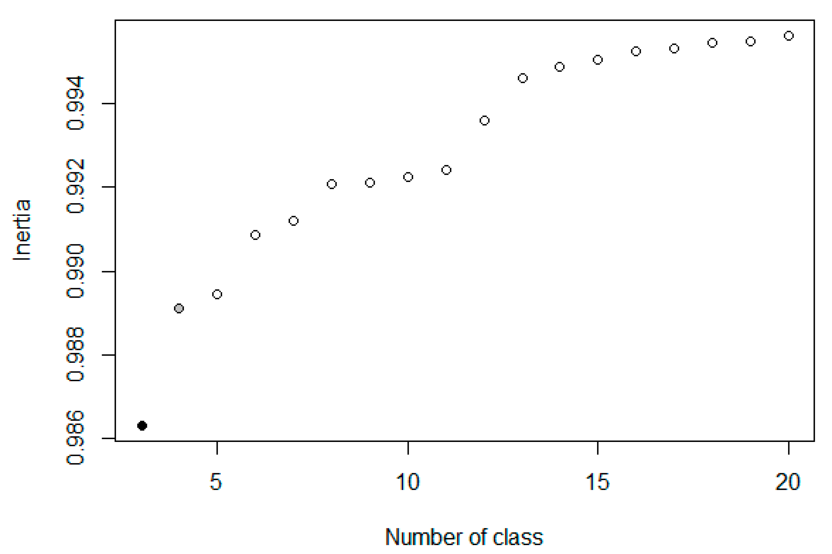
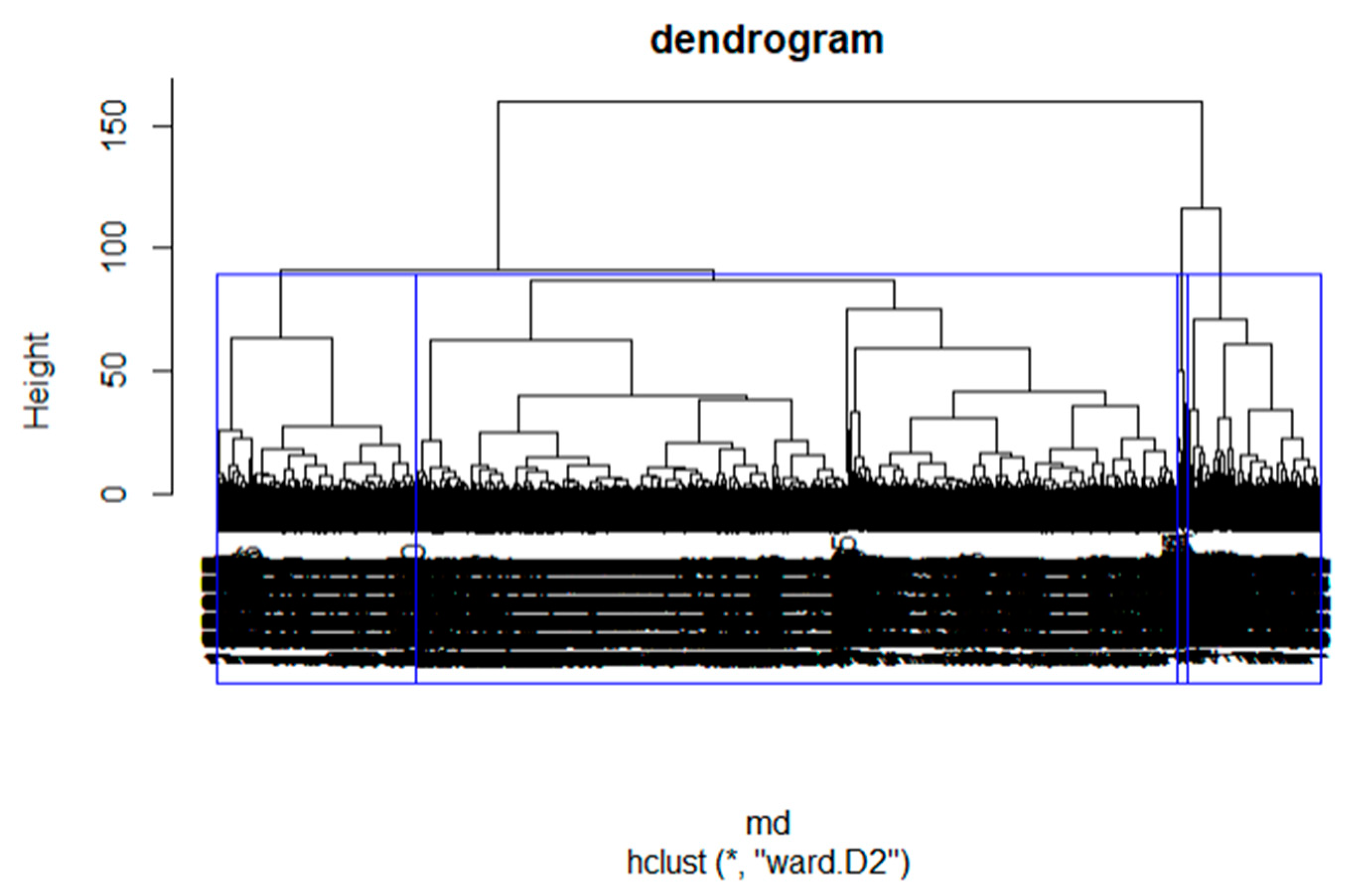
Only observers with at least two recording days and five observations were retained for analyses, i.e., 5896 observers out of a total of 9878. The objective of these thresholds was to retain only observers who had shown a certain commitment to the program. Following this, we explored similarities and differences in observation habits using hierarchical cluster analysis (HCA) and Ward’s minimum increase of sum-of-squares (of errors) method, without predefining a number of desired clusters. Observer profiles were identified from the dendrogram by analysis of inertia. We used the partitioning with the greatest relative inertia loss, identified with hierarchical clustering on principle components (HCPC).

2.3. Mapping the Naturalness Index (NI) of the Study Area

In order to interpret the spatial distribution of the recording, we chose to focus on the degree of naturalness of the landscape (naturalness index). This integrated method positions landscapes on a relative, quantitative scale ranging from “pristine” to “urban” [36] or more simply from “wild” to “not wild” [37]. This replicable method for assessing landscape quality has been used in numerous studies worldwide [37,38,39,40] and it includes most of the spatial variables already tested and cited in the introduction (proximity, accessibility/remoteness, habitat quality) facilitating comparisons with other work.

To quantify and map the naturalness index of the landscape, we adapted previous methodology [37,40,41] to our regional context and to the available spatial data. Among the four attributes generally used, we retained three: hemeroby of landcover (also called naturalness of landcover), human impact on landscape, and remoteness from road access. The fourth attribute, ruggedness, was excluded from our study because it was not relevant for the landscapes of our study area which are generally low-lying (maximum 416 m above sea level).

2.3.1. Landscape Hemeroby

The hemeroby concept provides a measure of anthropogenic impact on landscapes and habitats using a scale, in which the highest values (ahemerob) correspond to “natural” or undisturbed landscapes while artificial landscapes obtain the lowest values (metahemerob) [42,43]. To use the most recent and accurate data, a composite land cover map from different thematic datasets related specifically to natural and semi-natural vegetation, agriculture, forests, rivers, and human infrastructure was created. The details of the data used are given in Appendix B. To create the composite layer map, each dataset was first rasterized at 20 m then reclassified on a hemeroby scale and finally aggregated with the other data, giving priority to the most precise and recent data in cases of overlapping. For hemerobic reclassification, we applied a predefined hemeroby scale of landcover [43,44,45] which we adapted to our landcover dataset. The hemeroby scale ranged from level 6 (“ahemerob”, i.e., no human impact) to level 1 (“metahemerob”, i.e., destroyed, originally biocenosis). For each hemerobic level (1–6), we applied a second level of precision (1.1, 1.2, …) in order to consider the precision of the dataset used. The second level of hemerobic classification was based on local, expert knowledge. The complete table of hemerobic reclassifications is given in Appendix C. To account for the influence that the pattern of land cover immediately adjacent to the observer has upon hemeroby, the average hemeroby score of all cells within 250 m of the target cell was calculated as proposed by [37]. The final hemeroby scale ranged from 1 to 255.

2.3.2. Human Influence on Landscape

The “human influence on the landscape” attribute was quantified and mapped by two human presence proxies: human population and modern human artefact density. Similarly to Müller et al. (2015), we first used human population density as a proxy for human influence on landscape. To measure the population density, we used “Filosofi” data, which are the most precise population data available in France, collected at household level. To guarantee personal confidentiality, the French national institute of statistics and economic studies (INSEE) makes the data available in aggregate form on a 200 m grid. We used the Filosofi dataset for 2016, rasterized at a resolution of 20 m. The modern human artefact indicator refers to the quantity of artificial structures within the visible landscape, including railways, pylons, buildings, and other built structures. Similarly to [37], a number of modern human artefacts were extracted from the BD TOPO (IGN) and aggregated in a single dataset. The density calculation of the human modern artefacts area was performed with the focal statistic tool (ESRI, ArcGIS Pro 2.). For each cell, this tool calculates the location of a statistic in the neighborhood of a radius of 500 m circle (0.7854 km²). The radius of the moving window was chosen by an empirical method and according to [46]. We first tested three radial distances (500 m, 1 km, and 2 km) and kept the best compromise between visual representation and the normal distribution of the resulting data. The modern human artefacts map result is expressed in area of built-up land per square kilometer. The two layers were aggregated with equal weighting and reclassified on a relative scale from 1 to 255.

2.3.3. Remoteness from Roads and Paths

Remoteness from access is a very common indicator of naturalness maps (e.g., [37,38] and [40]). Remote areas are important both for species sensitivity to human presence and disturbance [47] and for the opportunity of solitude which some observers may seek [48]. We calculated the Euclidean distance in meters from all roads and paths including a buffer of 1 km around our study site. Only motorways were not considered because we assumed that it was not possible to go walking from these fenced roads. The remoteness from access layer was reclassified on a relative scale from 1 to 255. To produce the final map of naturalness index, we computed the sum of the three layers (hemeroby of the landscape, human influence on landscape and remoteness from access) with equal weighting. The final map had a resolution of 20 m and the naturalness index ranged from 1 (minimum naturalness index) to 255 (maximum naturalness index). All spatial analyses were carried out with ESRI ArcGIS pro 2.7.

2.4. Statistical Analyses

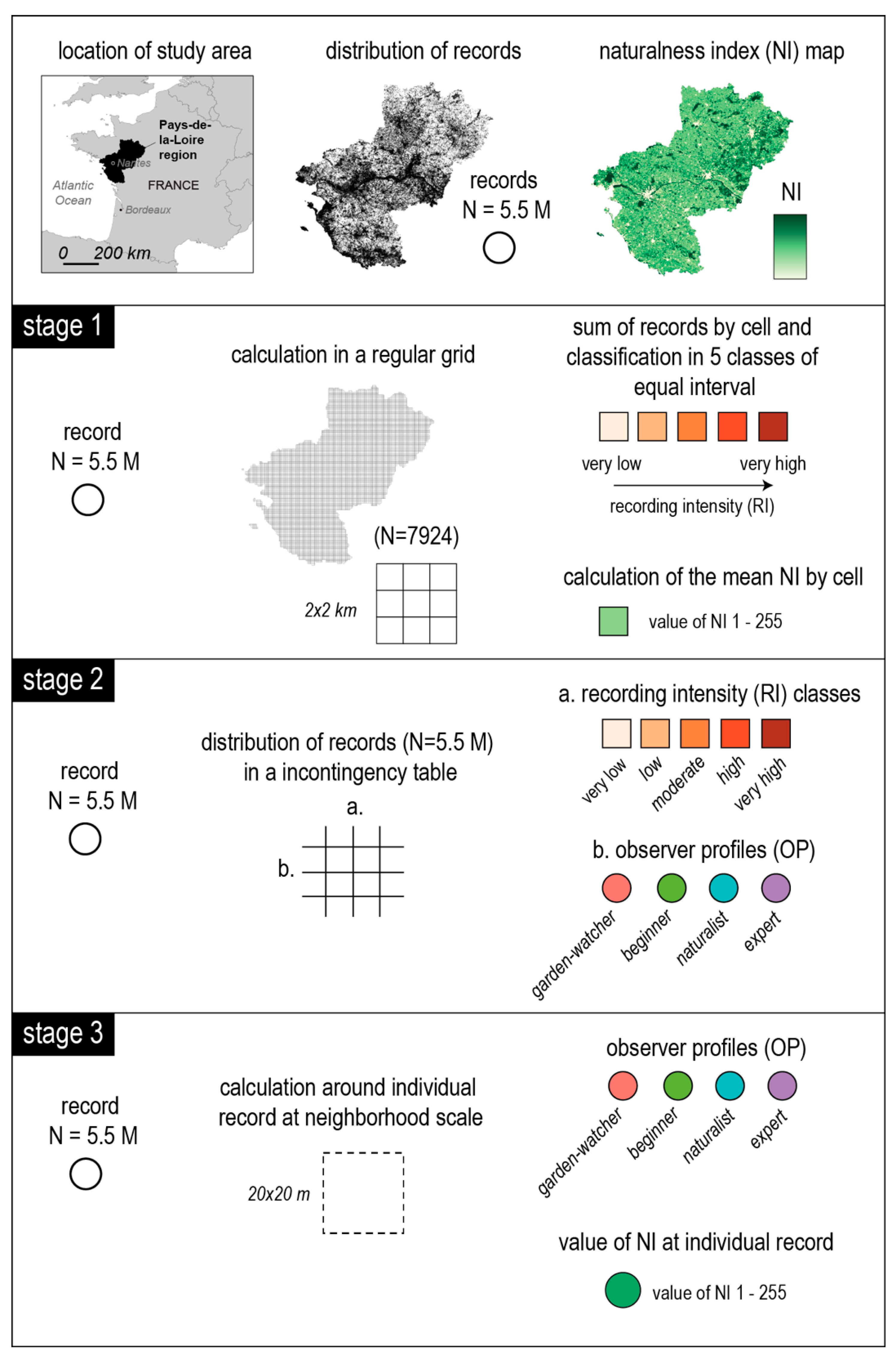
An illustrated workflow of the data analyses is given in Figure 1.

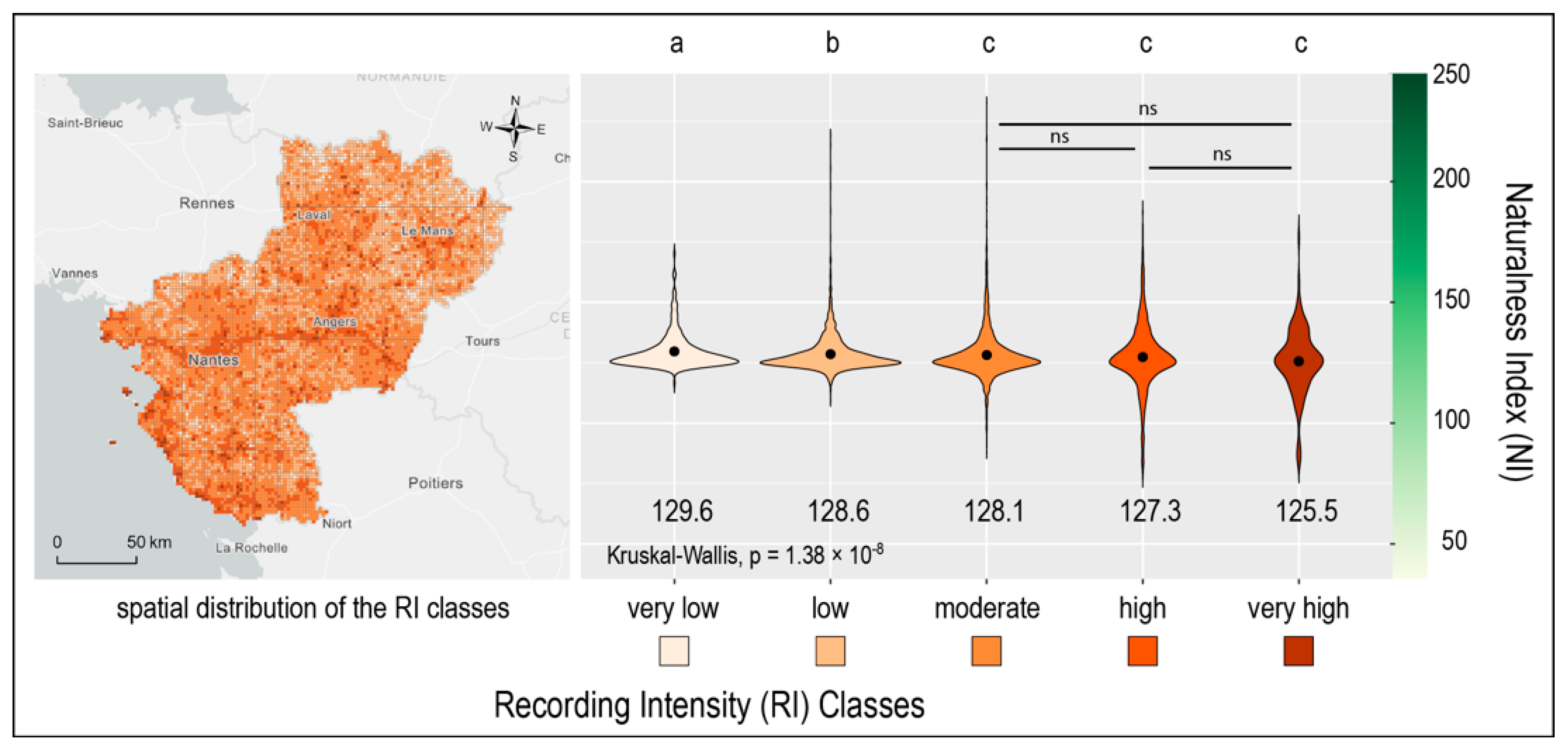
2.4.1. Testing the Effects of Naturalness Index on the Spatial Distribution of Recordings, at Regional Scale

Using GIS, a pre-existing 2 × 2 km grid used for French bird atlases was retained for the analysis across the study area; cells encompassing less than 80% of regional land cover (mainly boundary cells) were removed, leading to a grid of 7924 cells. First, mean naturalness index (NI) was calculated for each cell. Second, the exact locations of bird records were intersected with the regular grid (Figure 1). The number of records was calculated within each cell and all cells were then divided into five classes of recording intensity (RI) of equal intervals ranging from very low recording intensity to very high (Figure 1). We retained five classes which corresponded to the best compromise between a sufficiently large number for the analysis but small enough to guarantee a good, visual mapped representation. Moreover, because only a few cells had a very large number of records, the RI were log transformed to perform the classification with a normalized data set. In order to test the effect of NI on RI classes, differences in mean NI between classes of log RI were tested using non-parametric Kruskal–Wallis (KW) tests because of heteroscedasticity of the data (Figure 1). Differences in mean NI were tested between each combination of RI classes with Dunn’s post-hoc test of multiple comparisons using rank sums. We used Bonferroni method to adjust the p-value for multiple comparisons.

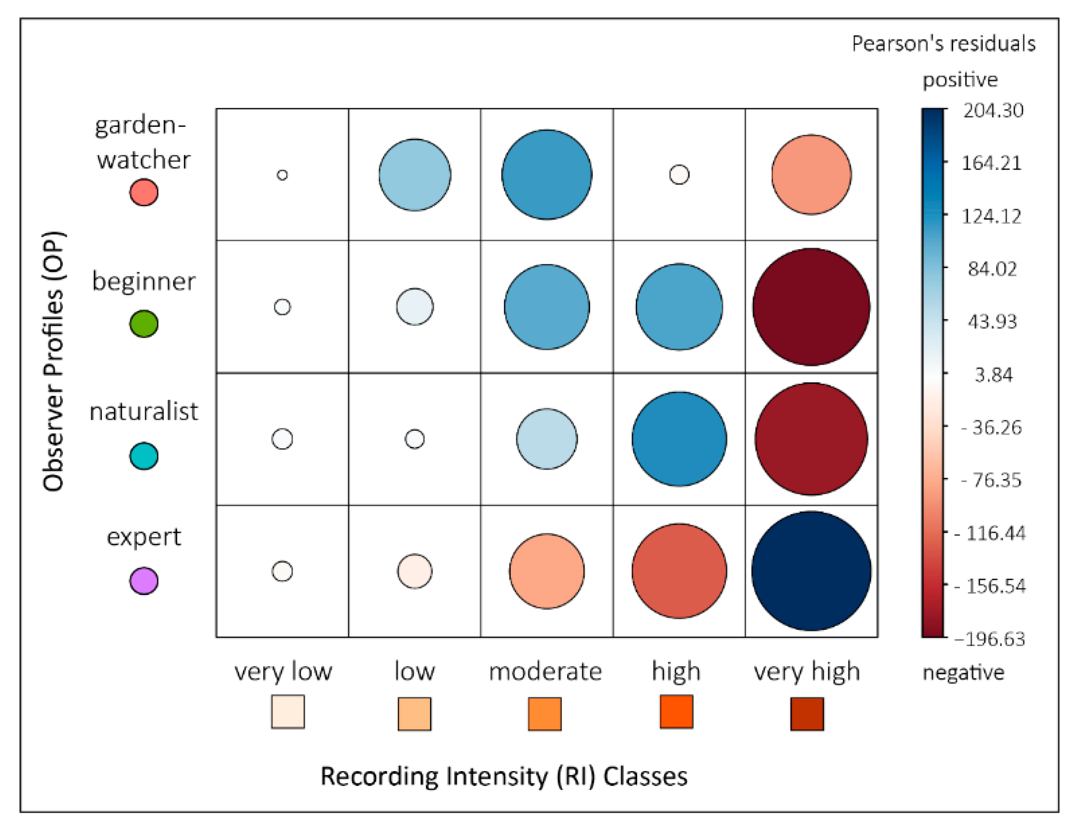
2.4.2. Testing the Hypothesis of a Homogeneous Distribution of the Records among Observer Profiles and Recording Intensity Classes

To test the hypothesis of a homogeneous distribution of the records according to observer profile and RI class, a Chi square test was applied on a contingency table. This table gathers the number of records of each observer profile in the different classes of RI. In order to interpret the intensity and the direction of each relationship (positive or negative), Pearson residuals were calculated and plotted.

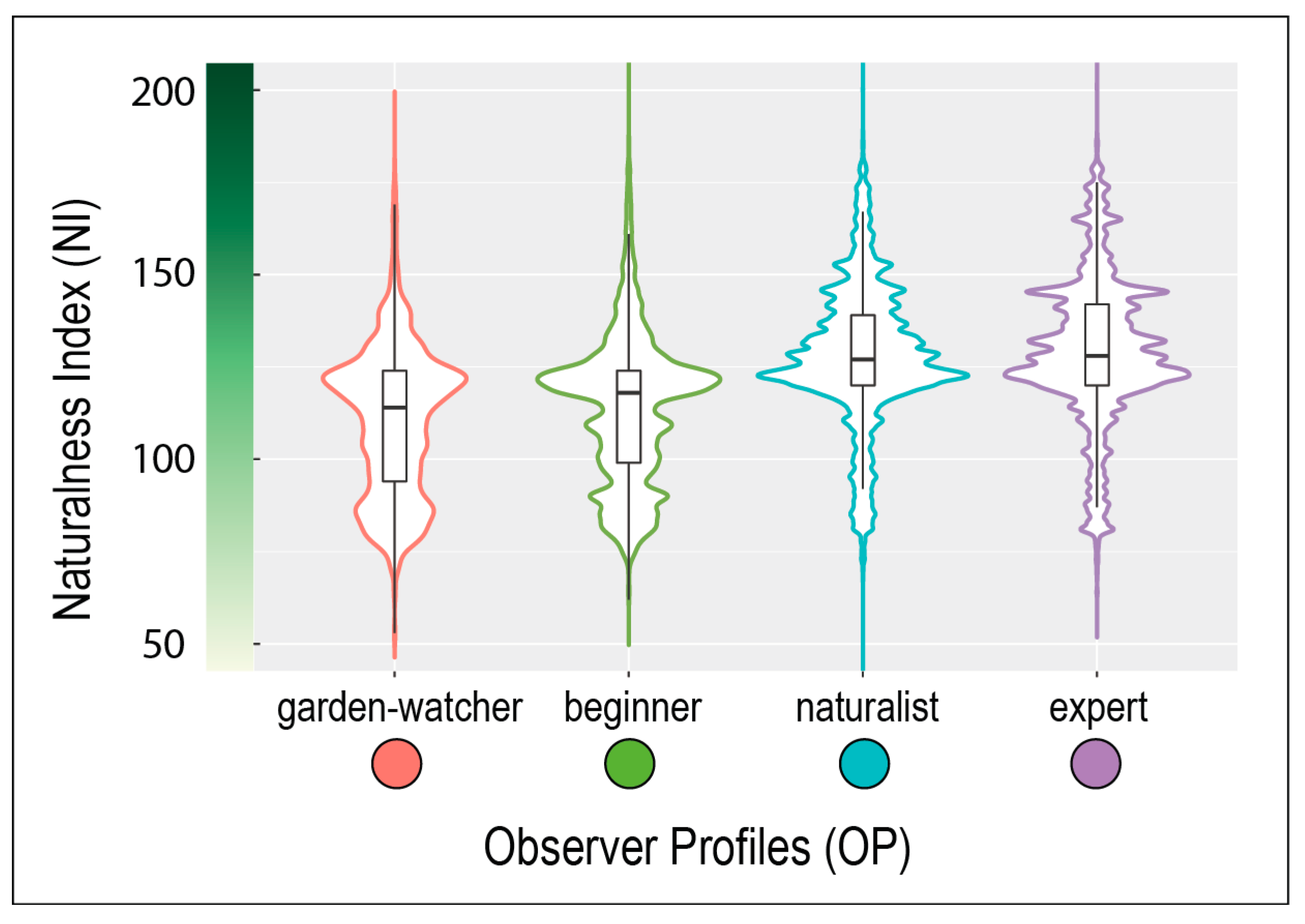
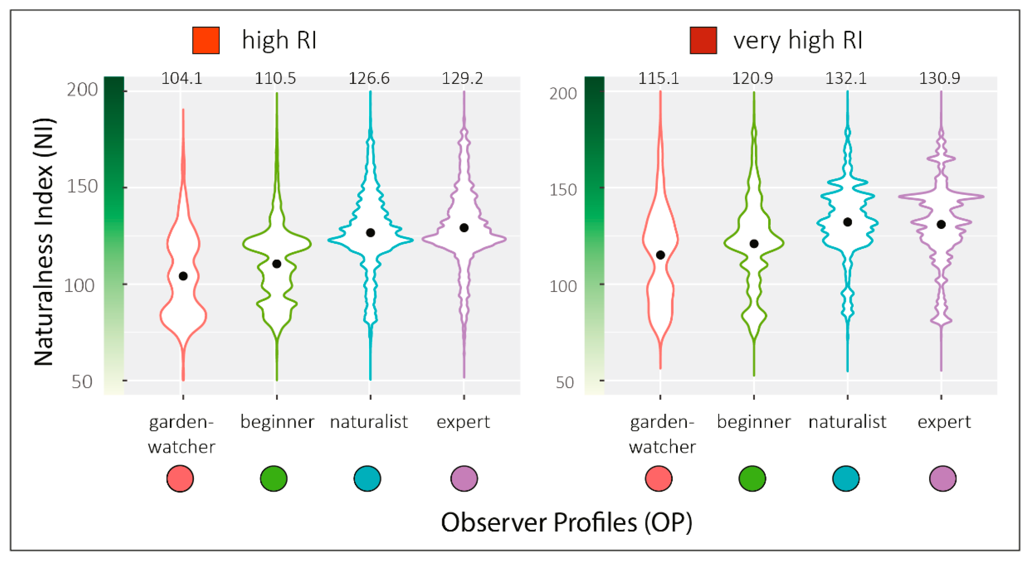
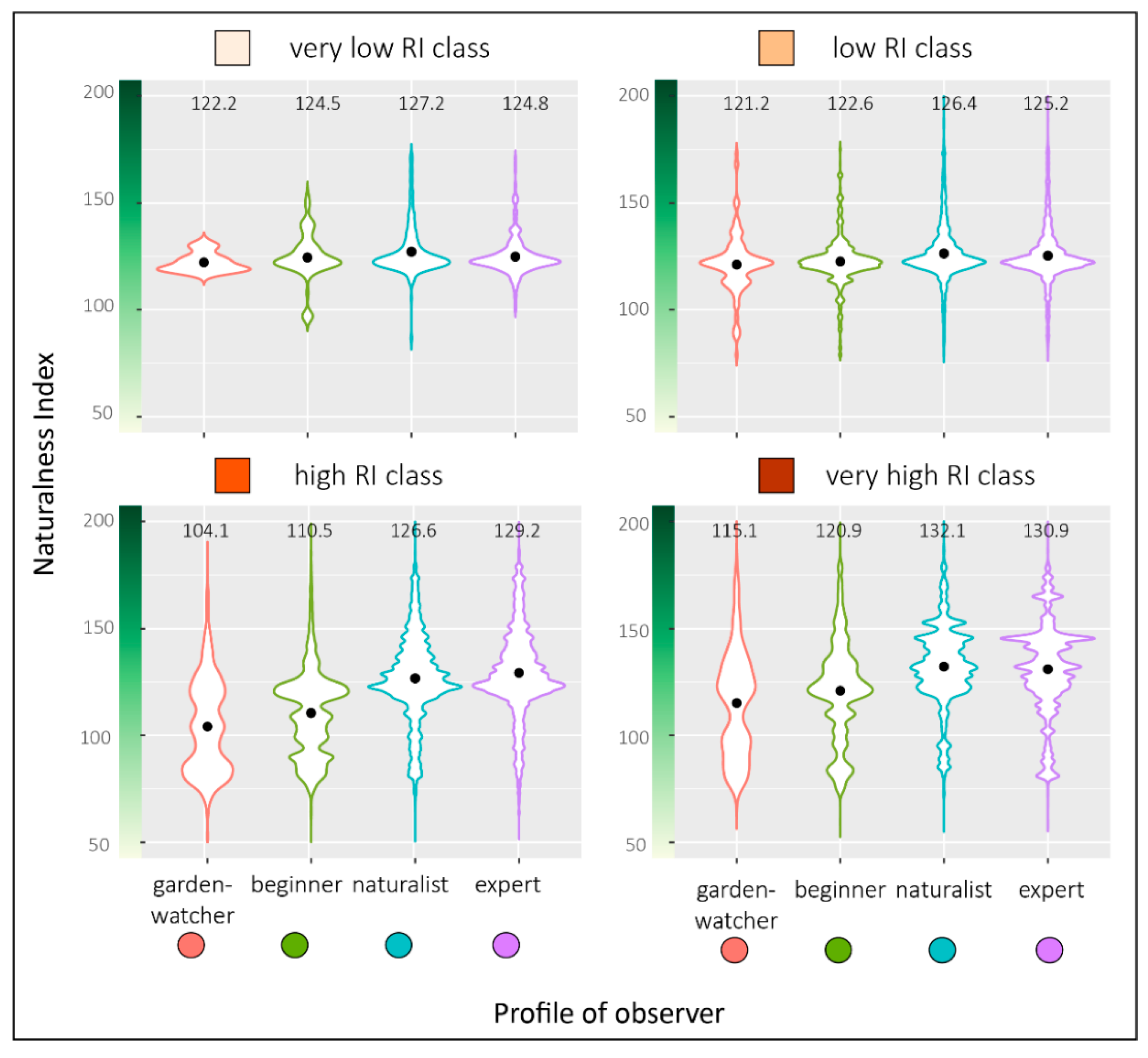
2.4.3. Testing the Effect of the Naturalness Index on the Recording Intensity of Observer Profiles at the 400 m² Record Neighborhood Scale

To test whether naturalness index (NI) in the neighborhood of bird records could explain recording intensity of the different observer profiles (OP), we calculated the mean NI of the total records for each OP. Contrary to Section 2.4.1, NI was calculated at bird record scale in order to directly consider the neighborhood around each recording point (and not at the scale of the 4 km² grid). For this, we used the highest resolution of the NI map which is 20 m (i.e., 400 m²). For each OP, mean NI of record neighborhoods were presented in violin plots to reflect the full distribution of the data, smoothed by a kernel density estimator.

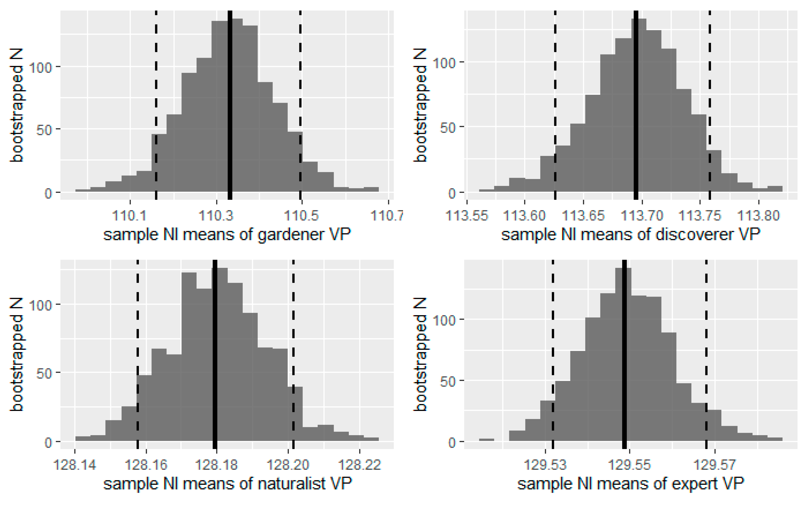
We then estimated a confidence interval (CI) of the NI means by bootstrapping method replication. For each OP, we resampled, replacing the original samples 999 times. We used the one.boot and perc function of the “simpleboot” R package for bootstrapping the mean statistic and extracting the CI at 95%. We then plotted the distribution of NI means as a histogram and added the initial sample NI mean and the CI boundaries (p = 0.05) for each of the four OP.

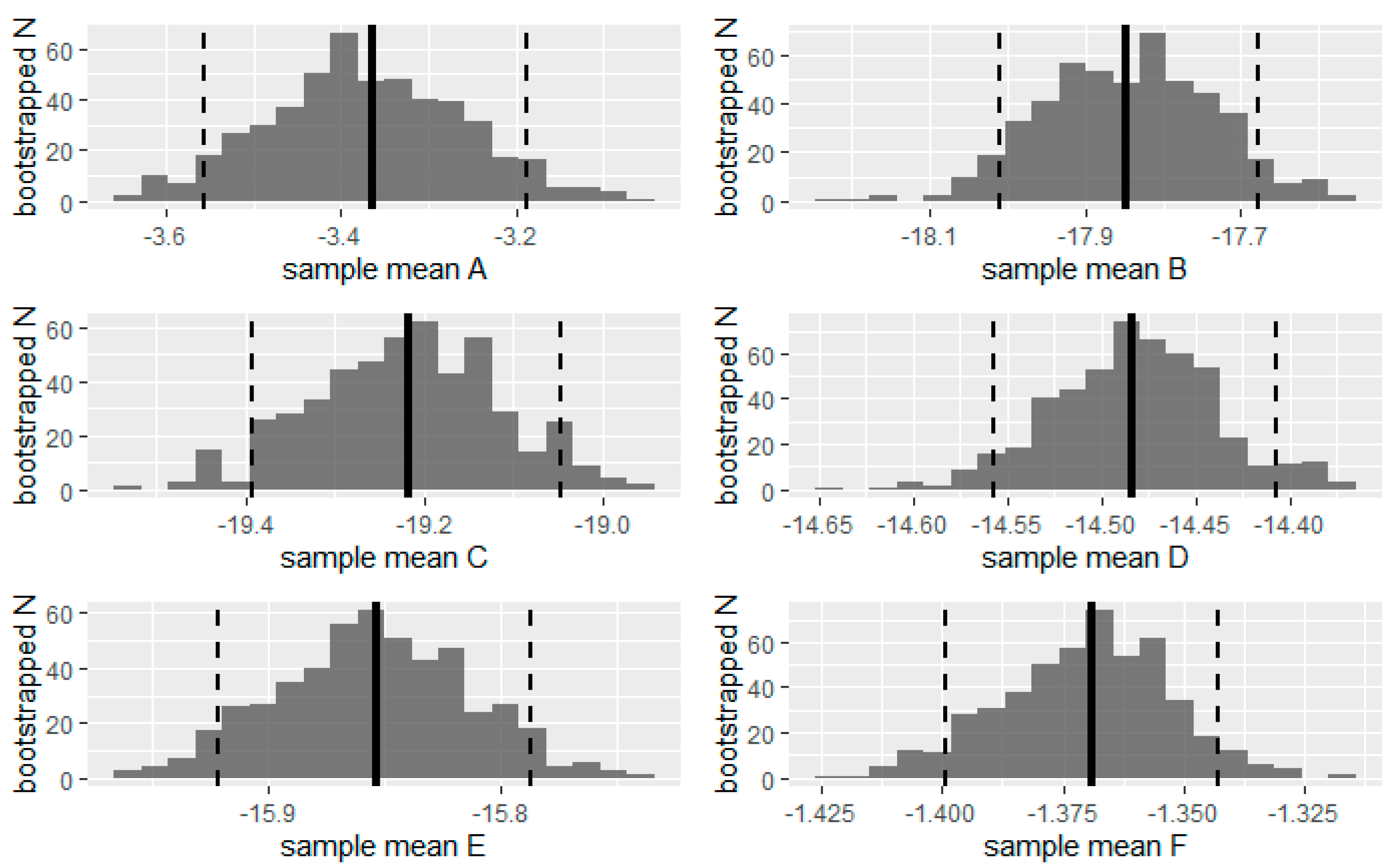
To test the differences in mean landscape NI between the OPs, we also calculated the CI for the pairwise comparisons. We used the two.boot function from the “simpleboot” package to bootstrap the difference between means of OP with 500 resamples and extract the CI at 95%. This number of bootstrapping was the maximum supported by the memory of our computer given the size of the original samples. We then plotted the distribution of differences as a histogram and added the initial sample mean and the confidence interval boundaries (p = 0.05) for each of the pairwise comparisons.

Finally, to ensure that the observed differences were not linked to the lack of data in some parts of the study area, this analysis concerned only the high and very high RI classes.

In addition to the R functions and packages already mentioned, we also used the following packages for our analyses and graphs: “ade4”, “corrplot”, “ggplot2”, “ggpubr”, “graphics”, “questionr”, “rstatix”, “vcd”.

3. Results

3.1. Four Observer Profiles

We found that the 11 metrics used to describe observer habits clustered participants into four distinguishable groups. Inertia analyses revealed that this classification best optimized the trade-offs between the number of groups and the within group sum of squares. The dendrogram of the distance matrix of records and the analysis of the loss of relative inertia as a function of the number of groups are given for information in Appendix A (Figure A2 and Figure A3).

Based on analysis of each group’s metrics we named the four observer profiles as follows: “garden-watchers”, “beginners”, “naturalists”, and “experts” (

Table 2. A summary of variation in metrics between observer profiles across the dataset as a whole. N.B. All 15 years of data over the entire region are pooled in this analysis. When mean is given, standard deviation is added as (sd).

		Observer Profiles
Metric Code	Metric Full Name	Garden-Watchers	Beginners	Naturalists	Experts
NO	Number of observers of this profile	1207	2741	1812	136
%O	Percentage of observers of this profile	20.47	46.49	30.73	2.31
NR	Total number of records contributed by this profile	36,741	234,281	2,244,306	3,665,869
%R	Percentage of records contributed by this profile	0.59	3.79	36.31	59.31
T1	Mean number of recording days per observer	4.68 (4.46)	15.30 (33.99)	133.32 (239.93)	1578.66 (929.48)
T2	Mean recording day frequency per observer	238.05 (265.16)	28.02 (46.94)	86.80 (105.03)	4.92 (11.02)
T3	Mean recording effort per observer	7.14 (3.78)	5.31 (3.42)	11.30 (13.29)	17.1 (13.30)
T4	Percentage of records made during the week	20.69 (23.8)	70.41(22.20)	60.56 (23.94)	64.33 (12.45)
S1	Mean spatial amplitude of record (km2)s	1.86 (2.29)	4.43 (6.61)	45.27 (57.63)	427.08 (214.65)
S2	Spatial density of records	2.20 (10.39)	6.65 (21.34)	41.05 (149.02)	2.55 (4.46)
S3	Minimum geometric extent	6.39 (8.52)	27.39 (50.49)	464.60 (352.78)	1982.24 (543,557.36)
C1	Mean number of records per observer	30.43 (29.01)	85.47 (30.44)	1238.57 (2647.86)	26,954.91 (30,357.36)
C2	Mean species richness per observer	14.78 (7.88))	19.67 (16.10)	87.97 (61.47)	257.38 (55.64)
C3	Mean Species Generalization Index (SGI)	29.36 (2.96)	29.29 (4.03)	30.67 (2.08)	30.45 (0.63)
C4	Mean Species Synanthropy index (SSI)	42.22 (14.45)	36.23 (24.10)	16.17 (11.26)	17.68 (8.28)

).

3.1.1. Garden-Watchers

Garden-watchers represented 20.47% of observers and only 0.59% of total records. Garden-watchers had few recording days, which were widely spaced in time but very spatially concentrated (less than two 4 km² cell on average). Members of this group were not necessarily beginners (they had been registered for more than 2 years on average), the vast majority recorded mainly at weekends (80% of records), and mostly synanthropic species.

3.1.2. Beginners

The beginners represented the biggest group in terms of numbers of observers (46.49%) but collected only 3.79% of total records. They were new to CS; they had been registered on average less than a year but had a fairly high level of activity. On the other hand, they made only a few records per recording day. The records were distributed among 4 km² cells on average; they were therefore not limited to the home base but covered a small part of the study area. The beginners were clearly distinguishable from the other profiles by a minority of records made during the week (20.69%). Finally, the species observed were on average less generalist than the other groups (generalization index = 29.29) but relatively synanthropic (index of synthropy = 36.23).

3.1.3. Naturalists

Naturalists formed around a third of observers (30.73%) and a third of records (36.31%). These were experienced observers, who had been registered for an average of 5 to 6 years. Their observations were distributed among 45.27 4 km² cells on average. This suggests naturalists observe not only around the home base, but also at a fairly stable list of sites, since the density of records is much higher (41.05) than for the other observer profiles. Finally, this was the profile with the lowest mean of synanthropic species records but the highest mean of generalist species records.

3.1.4. Experts

Only a small proportion of observers (136 observers i.e., 2.31%) formed this group but they collected the majority of all records (59.31%). They were distinguished by their seniority (registered10 years on average) and a large number of recording days (mean = 1578). They recorded the most frequently (every 4 or 5 days) and made many recordings per day. They covered an average of 427 cells (i.e., 10 times more than the naturalists). In addition, they recorded both rare and common species, more closely resembling professional, protocoled recording. They recorded a large number of species but the birds observed were often generalist species (SGI = 30.45).

3.2. The Naturalness of the Pays-de-la Loire Region

At the scale of the Pays-de-la-Loire region, we found an average hemeroby of 127.28 (sd 60.11), an average human influence of 247.23 (sd 12.01), and a remoteness from access of 7.26 (sd 8.16). With an aggregation of the three attributes, we created the naturality index (NI) map (Figure 2). We found an average NI of 128.15 (sd 14.48). However, NI is far from homogeneous across the study area. We found a higher NI on the eastern and northern part of the territory (dark greens patches are mainly forest areas) and along the Loire river (with lakes and associated wetlands). Conversely, the patches of low naturalness index corresponded to the region’s main cities: Nantes (to the west), Angers (to the east), Laval (to the north west), and Le Mans (to the north east).

3.3. Mean Naturalness Index (NI) Varied between Classes of Recording Intensity (RI)

Mean NI differed significantly between classes of RI (KW, P = 1.38 × 10⁻⁸). Less-visited areas had higher mean naturalness than intensely visited areas (

Table 3. Descriptive statistics of records in each RI class.

Classes of RI	Log Values of RI	Number of 2 km2 Cells (n)	NI Mean	NI Standard Deviation	NI Median
Very low	[0–2.228]	314	129.6	7.35	127.30
Low	[2.228–4.456]	2457	128.6	7.50	126.50
Moderate	[4.456–6.684]	3780	128.1	9.70	126.27
High	[6.684–8.912]	1239	127.3	13.03	126.58
Very high	[8.912–11.14]	134	125.5	13.40	125.90

). We found a mean naturalness of 129.6 (sd = 7.35) for very low RI class; 128.6 (sd = 7.50) for low RI class; 128.1 (sd = 9.70) for moderate RI class; 127.3 (sd = 13.03) for high RI class and 125.5 (sd = 13.40) for very high RI class.

Multiple comparison tests revealed that NI was significantly higher in classes of low recording intensity than in classes of high recording intensity. Except for very high/high, high/moderate, and very high/moderate pairwise combinations, all other combinations were significantly different (Figure 3 and Appendix D).

3.4. Numbers of Birds Recorded Varied among Recording Intensity Classes and Observer Profiles

The number of bird records differed significantly among RI classes and observer profiles (X² = 205,254, p < 0.05). The standardized Pearson residuals show strong associations (both positive and negative) between RI and OP. The expert profile showed a strong positive association with the very high recording intensity class whereas the three other observer types (garden-watcher, beginner, and naturalist) showed strong negative relationship with this very high RI class. Conversely, the expert profile was negatively related to high and moderate RI classes, whereas the naturalist and beginner profiles were positively associated with these two classes. Garden-watchers were also positively related to the moderate and low recording intensity classes (Figure 4 and Appendix E).

3.5. More Specialist Observers Record in Landscapes of Higher Naturalness Index

Depending on OP, NI varied in 400 m² landscapes neighboring bird records (Figure 5). We found a mean neighborhood NI of 110.33 [95% CI: 110.15–110.50%] for garden-watchers, 113.69 [95% CI: 113.62–113.76%] for beginners, 128.18 [95% CI: 128.15–128.20%] for naturalists, and 129.55 [95% CI: 129.53–129.57%] for experts. The histogram of mean NI and the CI boundaries (p = 0.05) obtained from the 999 bootstrapping resampling are available in Appendix F (Figure A4).

For the four OPs, we observed a majority of records in areas of intermediate naturalness. However, while garden-watchers and beginners recorded mostly in areas of low NI, these were the areas avoided by naturalists and experts.

We found the differences in NI to be relatively small between naturalist and expert records (1.37) as well as between garden-watcher and beginner records (3.37). In contrast, differences in NI were strong between naturalist—expert and garden-watcher—beginner. The plots of the six pairs of differences as histograms with the initial sample mean and the confidence interval boundaries (p = 0.05) are given for information in Appendix F (Figure A5)

Focusing on the most visited areas of the study site (high or very high recording intensity classes), we found that 4,465,633 records (corresponding to 80.86% of the total records) were concentrated in 5492 km² (corresponding to 17.32% of the study area). In these areas, we found that mean record neighborhood NI differed according to observer profile (Figure 6). In the high RI class, we found the same pattern as at the scale of all RI classes combined, i.e., mean NI increased from garden-watchers to beginners to naturalists and then experts. However, in the very high RI class, it was the naturalists’ records which had a higher mean neighborhood NI than the experts. The means of NI of the records of the four observer profiles are given for each RI class in Appendix F (Figure A6).

4. Discussion

4.1. Towards a Better Understanding of Observer Profiles

This study has built upon the framework proposed by [33], which uses clustering of temporal, behavioral metrics to distinguish the types of participant in environmental CS programs. We added spatial metrics and, as suggested by [28] and initiated by [7], we developed quality metrics based on indices of species specialization [49] and synanthropy [50] to better assess not only the numbers but also the types of bird species recorded by participants.

The four observer profiles we obtained are partially comparable with those of other studies. For example, the experts, who represented only 2.31% of the volunteers but 59.31% of records, could correspond to so-called “super users” described by [7]. Ref. [28] also found a repeated pattern across datasets and taxonomic groups of a few volunteers contributing many records and many volunteers contributing few records and this is referred to as the 80:20 rule [51]. In our study also, beginners contribute very few records but form the largest group of observers.

Using temporal metrics alone, ref. [28] distinguished three volunteer profiles: “dabbler”, “steady”, and “enthusiast”. By adding a “distance of recordings from home” spatial variable, ref. [34] distinguished “one-session volunteers” who travelled least and committed the shortest amount of time, “long-term volunteers” who travelled furthest and committed the most time and “short-term volunteer”, mid-way between the two other types. By introducing quality metrics in our study, we obtained classes that reflected not only differences in temporal and spatial engagement (e.g., sedentary garden-watchers versus mobile experts) but also differences relating to observer expertise (e.g., beginners versus naturalists).

Such groupings are useful in the case of CS programs with numerous and diverse participants, such as opportunistic bird CS programs. However, for other taxonomic groups and programs, dividing participants into clear types may not be appropriate. For example, ref. [7] suggested that volunteers in an opportunistic butterfly recording CS program could be classed along four continuous scales of recording intensity, spatial extent, recording potential, and rarity recording. Another important limit of profiling is that it is static whereas we can assume that volunteers will move from one profile to another over time. It is possible that beginners or garden-watchers will develop their skills through practice, observe more species, less generalist and synanthropic species, ultimately evolving to become naturalists or possibly experts.

Despite these limits and as demonstrated by [28], observer profiling can be used in comparisons between CS programs but also, as we have seen in this study, for analysis within a single CS program. It could also be useful for long-term programs that are experiencing a change in participant profiles. As mentioned by [31], there has been a noticeable shift toward people collecting and providing data with limited training and little or no direct social interaction with experts or other citizen scientists, before submitting them via an online reporting platform. In addition, during pandemic lockdowns certain forms of participation in CS increased, generating more data and more data heterogeneity. These recent and rapid transformations have sometimes taken managers of long-running CS programs by surprise, and they need tools to manage and analyze these new data. In this study we focused on how observer profiling can be used to better understand spatial biases in recording effort and intensity.

4.2. Spatial Bias in CS Recording Intensity at Regional Scale: Influence of Landscape Naturalness

At regional level, we observed that well-known spatial patterns explained variation in recording effort. Our results showed that the most frequented sites in terms of recording intensity (RI) had lower average naturalness index (NI) (lower than less frequented sites and even lower than the overall regional average). We also found that the most frequented sites (cells with high or very high RI) were close to towns and easy to access (i.e., close to roads) (see map, Figure 3). This result is similar to studies by [12,19,24,26,27], conducted at a range of spatial scales, in several regional contexts, and involving a diversity of CS programs (taxonomic groups, observer profiles). The tendency toward intense recording activity in accessible and urbanized areas therefore constitutes a relatively well-documented bias.

4.3. Relationships between Observer Profiles and Landscape Naturalness at Finer Scale

While regional scale recording intensity was mostly driven by spatial patterns of proximity and accessibility, a closer look at the scale of record neighborhood revealed different preferences in landscape naturalness among observer profiles. Thus, although all observer profiles mainly visited the same broad scale areas, they did not frequent the same sites within those areas. In areas of high or very high RI, experts and naturalists tended to seek areas of higher NI which was not the case for garden-watchers and beginners. The different profiles therefore appeared to complement each other in terms of spatial coverage. This result is of particular importance as it could be used by organizers of CS programs wishing to improve spatial homogeneity in recording.

4.4. Implications and Future Directions

Increasingly, knowledge of observer profiles is being used to improve CS data quality for analytical purposes. Commonly, data are filtered to reduce bias and improve subsequent predictive modelling of species distributions [52]. Correcting bias linked to variation in participant expertise has for example successfully been used to improve species distribution models based on CS data [53].

Knowledge of observer profiles could also help CS organizers to guide particular types of observer with known observing habits and spatial preferences toward areas which may be under-recorded. Completing existing CS databases with a more guided approach is often necessary before data can be fully exploited [52]. Such knowledge may also be used to adjust future recruitment strategies toward particular observer profiles, depending on program objectives.

It could be interesting to further analyze the reasons for observer profile preferences. A considerable body of literature is concerned with human perceptions of naturalness [38,54,55,56,57]. Interdisciplinary collaboration with the human and social sciences should lead to a deeper understanding of landscape preferences and related bird recording habits [58].

Since observer profiles in our study integrated spatial metrics, we have seen that part of the bias in recording is related to spatial distribution of naturalness gradient in our study area. The Pays-de-la-Loire region is relatively heavily urbanized with little or no wilderness. The population density is of 120 inhabitants/km², the road network is dense, and rural landscapes have been transformed by agriculture. In such contexts, the naturalness index (NI) is used to quantify a gradient of human modification the NI [59,60], and can enable us to highlight even subtle variation in human pressure [40] but no observer is ever completely remote from towns or roads. In other regional contexts landscape types, areas of high NI and species richness may be under-recorded, even by experts, due to very low accessibility [29]. CS programs should consider landscape configuration and areas of probable under or over-sampling, at the program planning stage.