Article

Sustainable Restoration of Degraded Farm Land by the Sheet-Pipe System

by
Koremasa Tamura
1,
Hiroshi Matsuda
2,*,†,
Budi Indra Setiawan
3 and
Satyanto Krido Saptomo
3
1
Kyouwa Corporation, Hagi 758-0061, Japan
2
Yamaguchi University, Ube 755-8611, Japan
3
Department of Civil and Environmental Engineering, IPB Kampus Darmaga, IPB University, Bogor 16680, Indonesia
*
Author to whom correspondence should be addressed.
Professor Emeritus.
Land 2021, 10(12), 1328; https://doi.org/10.3390/land10121328
Submission received: 22 October 2021 / Revised: 27 November 2021 / Accepted: 28 November 2021 / Published: 2 December 2021
(This article belongs to the Special Issue Water Resources and Land Use Planning)

Abstract

:
For the sustainable restoration of wet farm land degraded by the climate change-induced rise of ground water level (GWL) and soil salinity etc., the sheet pipe system is one of the most useful technologies which reduces cultivation obstacles due to the poor drainage by controlling the rapid drainage function and enabling farmers to produce profitable crops. This system is characterized mainly as a perforated polyethylene rolled-band sheet 180 mm in width and 1 mm thick which is drawn into the subsurface layer while transforming a drainage pipe with φ = 50 mm. The major advantage of this system is that since the sheet pipe is installed without trenching, the disturbance of land is minimized and the construction period can be shortened to about 1/4 (which reduces the cost approximately by 50%). In this study, by using the sheet pipe installed miniature-type model soil box, the drainage capacity of the sheet pipe was confirmed as being the same as the pipe-shaped standard drainage pipes. Based on the observations of the saturated–unsaturated flow and the maximum lowering rate of GWL was predicted. Finally, at the farm land wherein the free board of the adjoining canal was limited, the effectiveness of the sheet-pipe system was confirmed.

1. Introduction

For the sustainable restoration of farm land degraded by climate change-induced rise of ground water level (GWL) and soil salinity etc., the sheet pipe system is one of the most useful technologies. It reduces cultivation obstacles due to poor drainage by controlling the rapid drainage function and enables farmers to produce profitable crops [1,2,3,4,5]. Sheet-pipe-used drainage is also useful as a convenient way to improve the playgrounds, parks, golf courses, soft soil ground, etc.
Although subsurface drainage by the excavated mole drains is expensive and time consuming [6], the sheet-pipe system is characterized as another type of subsurface drainage in which the perforated high-density polyethylene rolled-band sheet with a width of 180 mm and a thickness of 1 mm (the length is 100 m/roll) is transformed to a drainage pipe with 50 mm in diameter just before being inserted into the subsurface soil layer by a ‘Mole Drainer’ (as shown in Figure 1 and Figure 2). So, the advantage of this system is that since the sheet pipe is installed without trenching and backfilling, the disturbance of the land is minimized and the construction period can be shortened to about 1/4 of the conventional method (which reduces the cost approximately by 50%). During the last two decades, an abrupt climate change induced upward movement of water level in areas with shallow water tables and coastal areas with water intrusion has resulted in root zone salinity [2]. To cultivate problematic lands sustainably, a proper water management system is required which keeps water levels in a preferable range for optimum plant growth.
The subsurface drainage method by using sheet-pipe has been developed more than 40 years ago in Japan for the relatively smaller lot of farmlands with about 3000 m2 as a standard size. After being certified as a new technology by the Japanese government in 2001, this method was gradually spread and adopted in the agricultural land improvement projects [4], and also by the observations at ten years after the installation of the sheet pipe, the deformation of pipe form and the significant clogging of the drainage holes were not confirmed [7]. Until now, however, and although the effectiveness of the sheet-pipe system was observed on the crop productivity in detail by measuring water depth, weather parameters such as solar radiation and temperature. etc. [8,9,10,11,12], reports on the differences of the flow capacity between the sheet-pipe and the standard slotted PVC or flexible pipes have been very limited [13] and the hydraulic properties of the sheet-pipe system have not been clarified satisfactorily, especially on the flow capacity of the sheet-pipe when installed horizontally in the ground.
In this study, to clarify the differences in the flow capacities between the sheet pipe and four other drainage pipes which are commercially supplied in Japan, miniature-type model soil box (hereinafter designated as MT-MSB), which is possible to measure not only the volume of water discharged through the sheet pipe but also the change of the hydraulic pressure in the soil layer, was newly developed [14], based on the assumption by Dupuit-Forchheimer (i.e., in a system of gravity flow toward a shallow sink, all of the flow is horizontal and that the velocity at each point is proportional to the slope of the water table but independent of depth) [15]. By the MT-MSB, the drainage capacity of the sheet pipe, the change of the water head, and the vertical distribution of matric suction were measured with time on natural fine sand (named Toyoura sand which is widely used in geotechnical engineering in Japan), and it is clarified that the flow capacity of the sheet pipe is almost the same as other drainage pipes and the storage coefficient was obtained. Based on the experimental results, for the case that the sheet pipe is laid horizontally, the maximum lowering rate of GWL was predicted by the intake model. Finally, as a field case study, the effectiveness of the sheet-pipe system was investigated by focusing on the differences between the water level in the canal and GWL at a paddy field which includes both a horizontally installed sheet pipe area and no sheet pipe area.

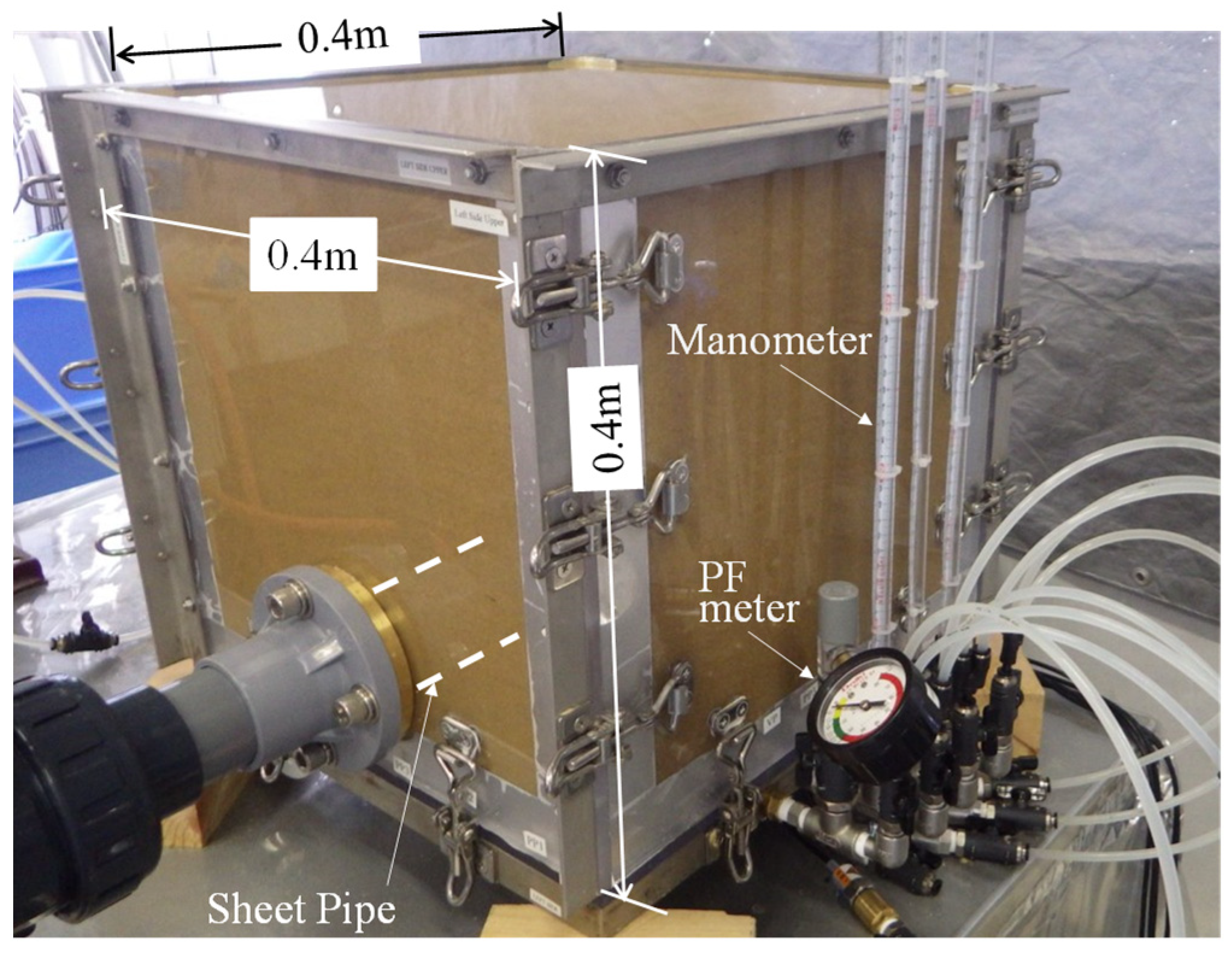
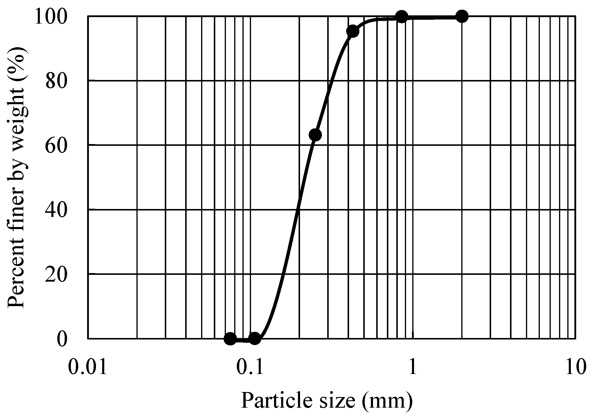
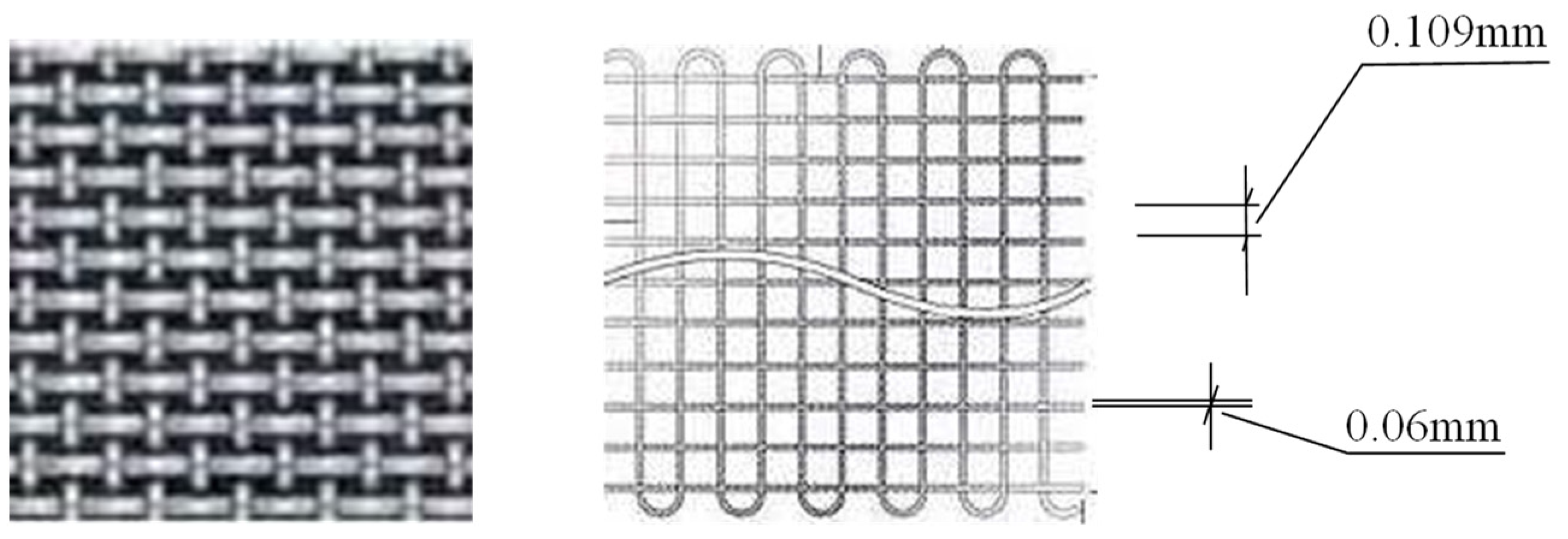
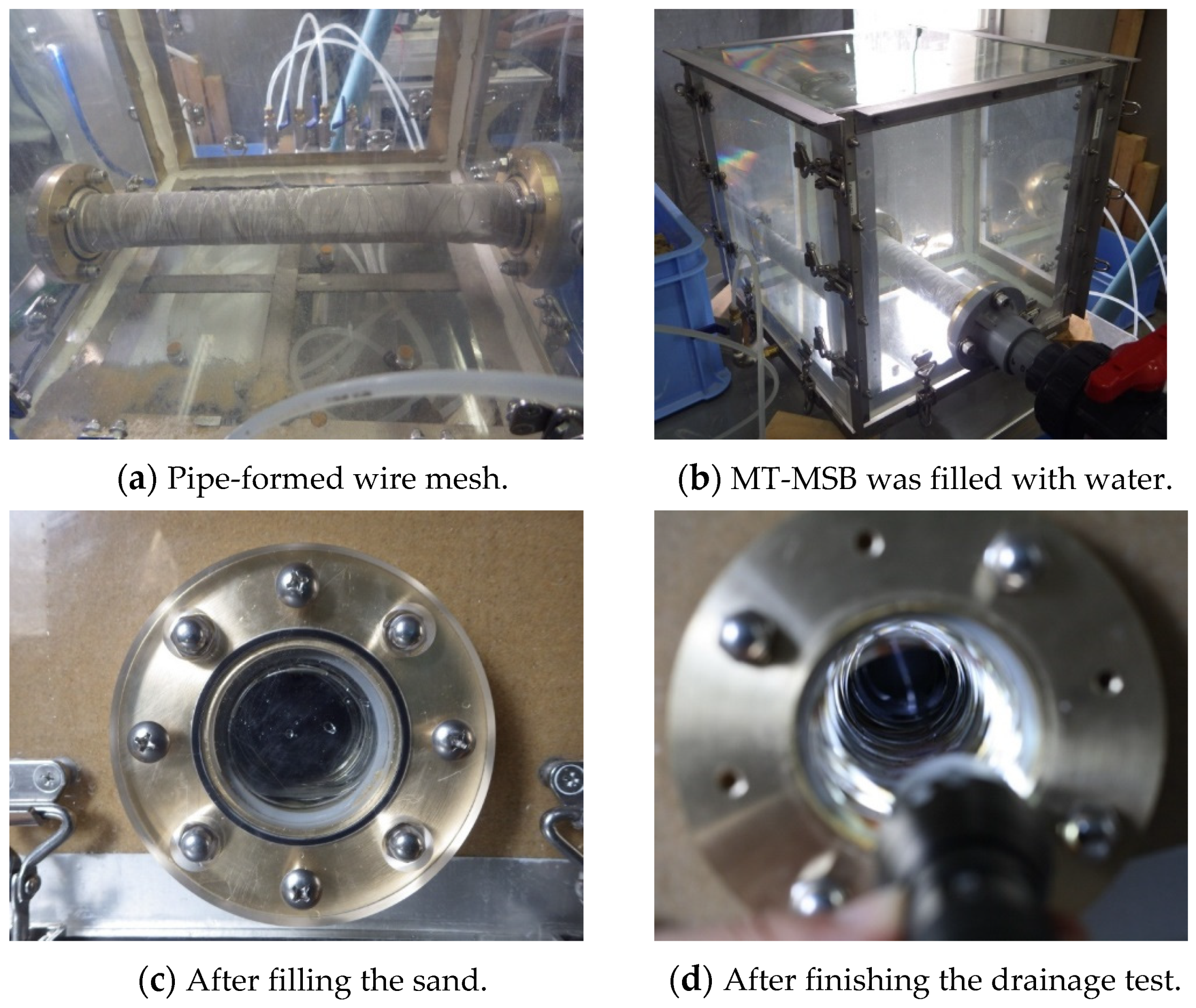
2. Materials and Methods

To find the differences in the drainage capacity between the sheet pipe and four other typical drainage pipes, MT-MSB (as shown in Figure 3) was developed. The dimensions of MT-MSB are 0.4 mW × 0.4 mL × 0.4 mH. For the assumption by Dupuit-Forchheimer as mentioned above, to satisfy the layer below the drainage pipe as impermeable, the drainage pipe was placed as close to the base plate as possible and through small holes on the base plate which were placed at 0.03 m(PP3), 0.10 m(PP2) and 0.17 m(PP1) from the center of the drainage pipe, the hydraulic pressures and water heads were measured by using the pressure transducers (PGM02KG) and manometers. As for the change of matric suction during the drainage test, the porous cup column was set horizontally at the depth 0.10 m, 0.20 m, and 0.30 m from the top surface of MT-MSB as shown in Figure 4 and the positive and negative pressures were measured by the pressure transducer (PGM1KG).
To fill the MT-MSB with soil sample and water, after deairing the predetermined weight of sample was poured into the MT-MSB with a sufficient depth of water step by step. To raise the water level in the MT-MSB, the water was supplied from the constant head water tank to the four small holes at the base plate in which porous stones are placed. MT-MSB filled with sand and water is shown in Figure 5. The volume of the water drained from the drainage pipe was measured with time by the volume-correlated load transducer (TCLA1KNB).
Since one of the main objectives of this study is to investigate the maximum flow capacity of the drainage pipe, as a relatively higher permeable soil than farmland soil, Toyoura sand obtained in Yamaguchi prefecture, Japan was chosen, which has been widely used previously in geotechnical investigations [16,17,18,19]. Its physical properties, including the coefficient of permeability and the particle size distribution curve, are shown in Table 1 and Figure 6, respectively. In Table 1, ρs is the particle density, emax and emin are the maximum and minimum void ratio, k is the coefficient of permeability and Dr is the relative density.
To confirm the applicability of the sheet pipe, the flow capacity was compared with those of four other drainage pipes. In Table 2, dimensions of drainage pipes including the sheet pipe (designated as Pipe A or Sheet Pipe A) are shown for the outside diameter, hole size, pipe thickness, and length. In these drainage pipes, B is the perforated PVC pipe, C and D are the slotted PVC pipe and E is the hard polyethylene pipe.
In the drainage tests, all the drainage pipes shown in Table 2 were covered with the wire mesh filter as shown in Figure 7 in which the opening and the wire diameter are 0.109 mm and 0.06 mm, respectively. This is due to the fact that the size of the drainage holes for every pipe with the range from 2 to 8 mm is larger than the maximum particle size of Toyoura sand.
Thus, the effects of wire mesh filter on the flow capacity were confirmed by the constant head permeability tests and also by using MT-MSB as follows. Firstly, to measure the flow capacity only through the wire mesh filter, after placing the sheet pipe which was covered with the wire mesh, the sheet pipe was pulled out from the window on the side wall of the MT-MSB as shown in Figure 8a. Secondly, MT-MSB was filled with water as in Figure 8b and the drainage test was carried out. Thirdly, MT-MSB was filled with sand and water as shown in Figure 5 and Figure 8c, then the water was drained out. Figure 8d shows the inside of the wire mesh filter after finishing the drainage test. It is seen that the shape is kept as those before the drainage and that no sand particles were confirmed.

3. Results and Discussions

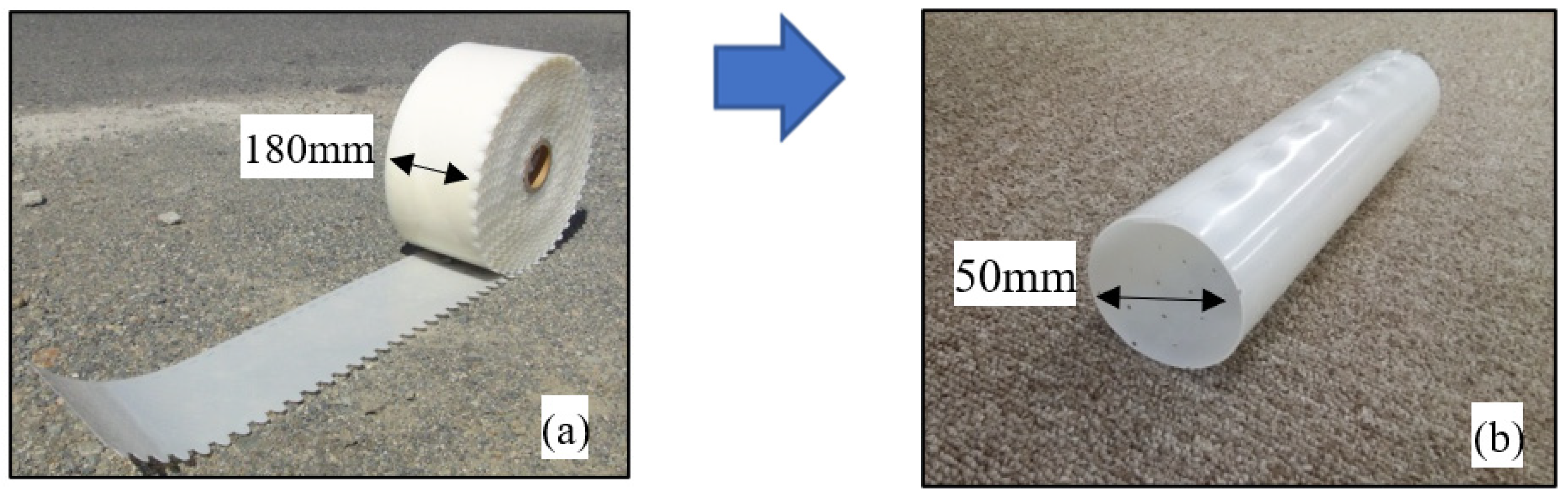
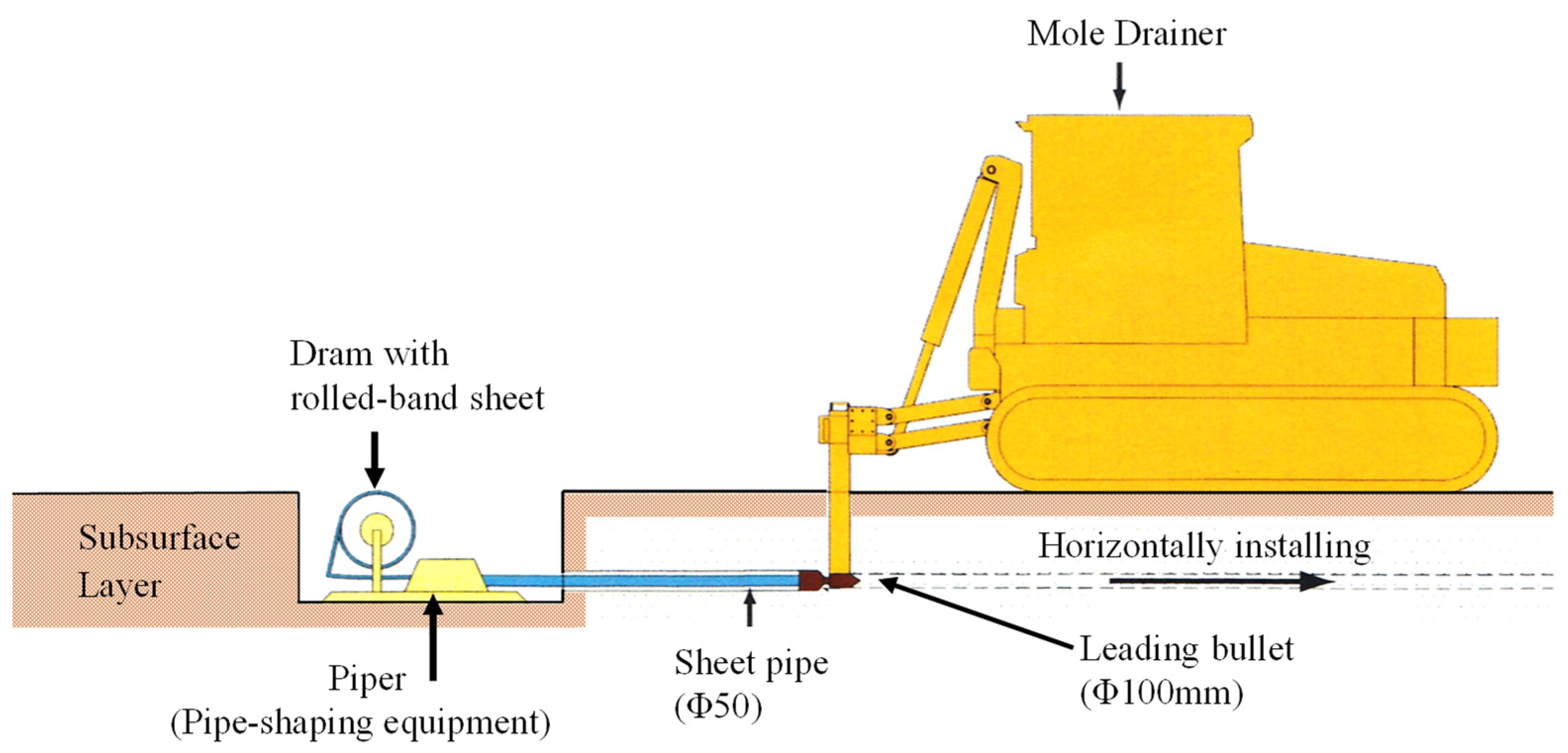
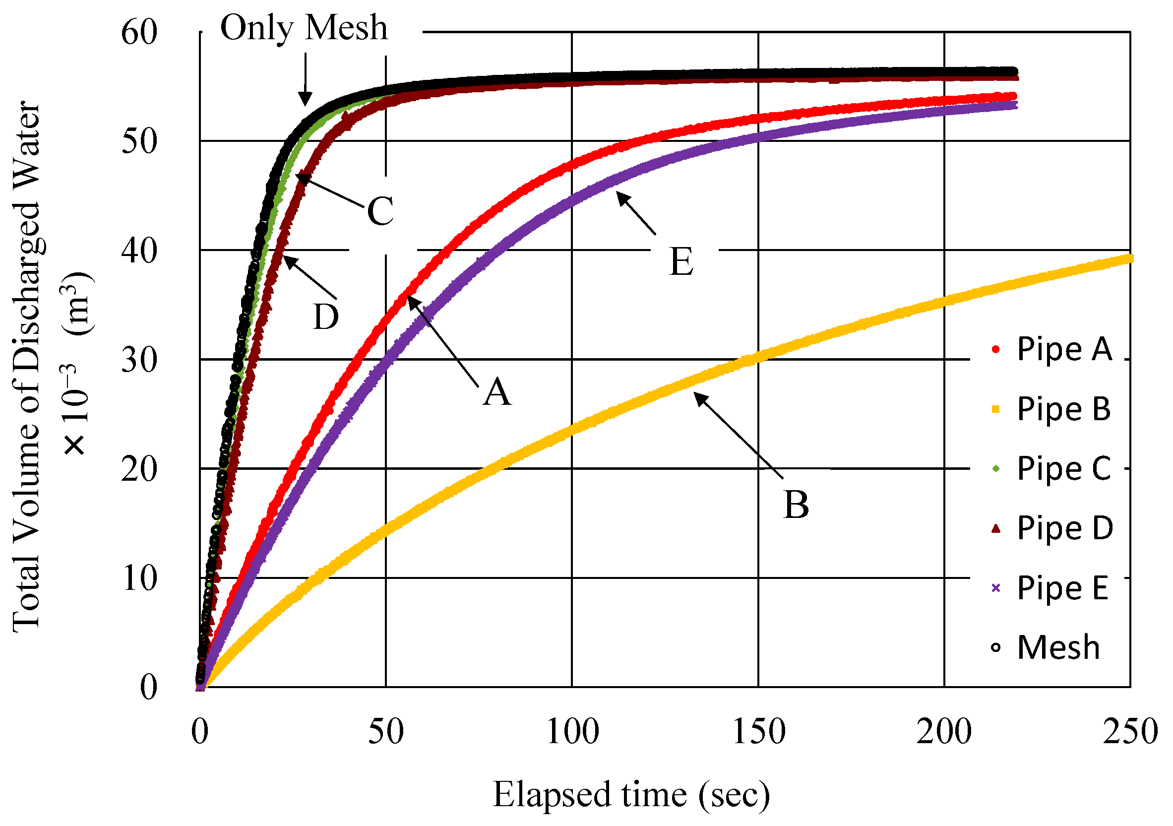
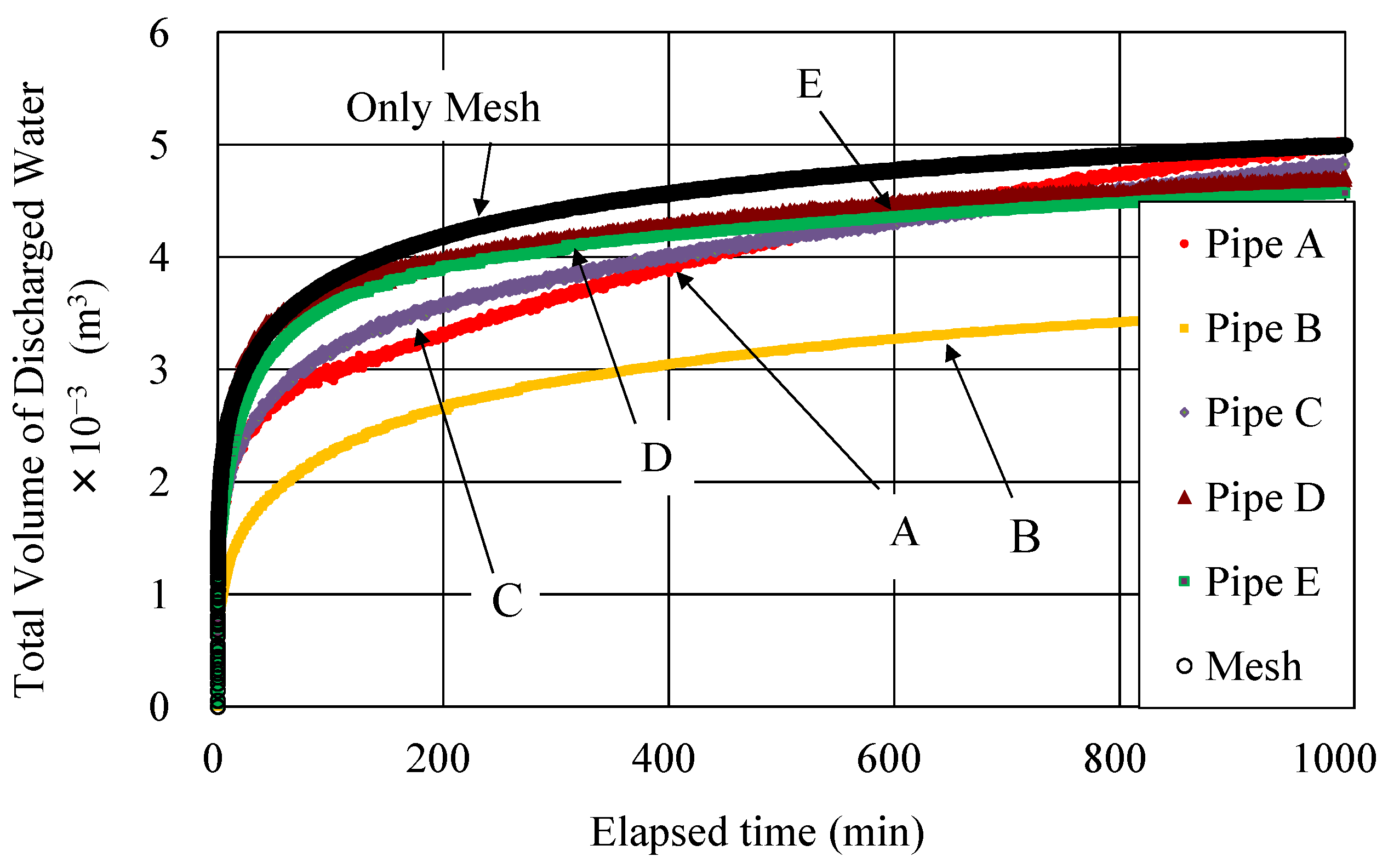
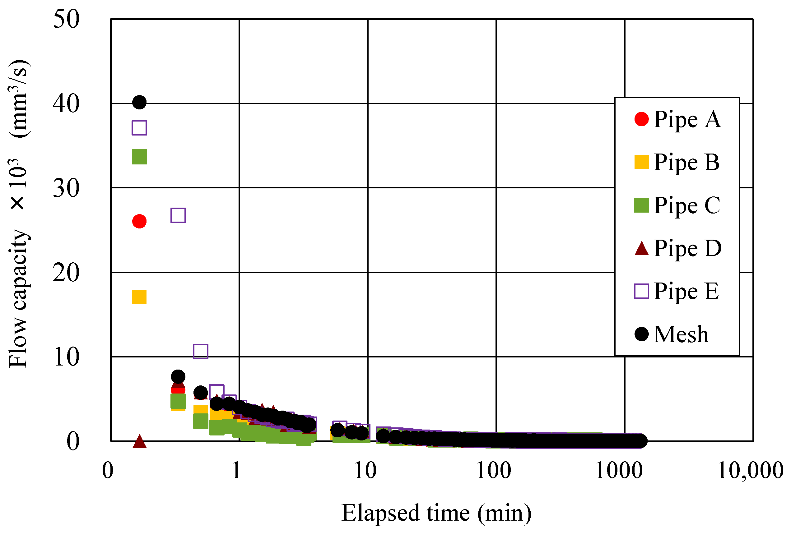
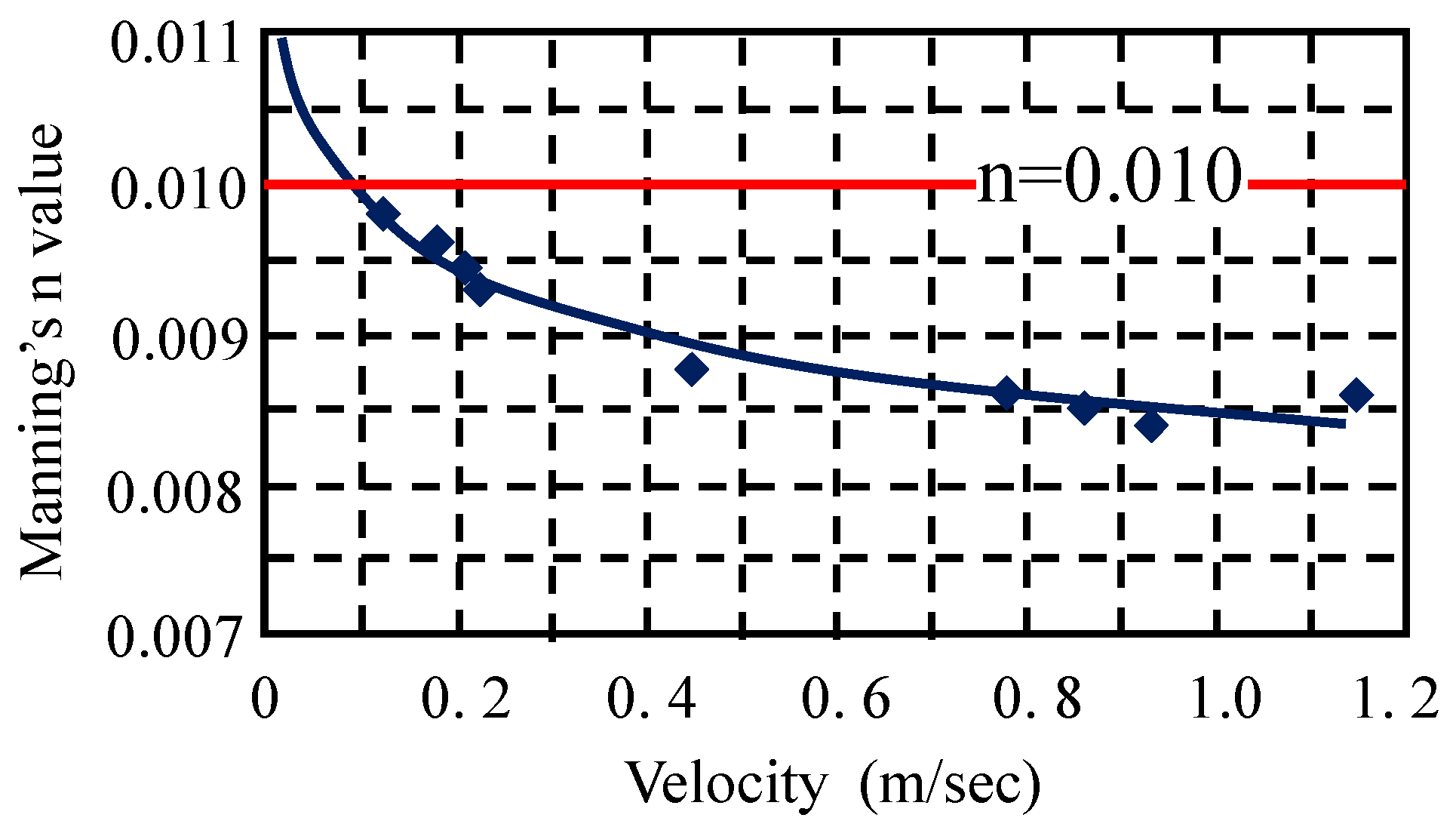
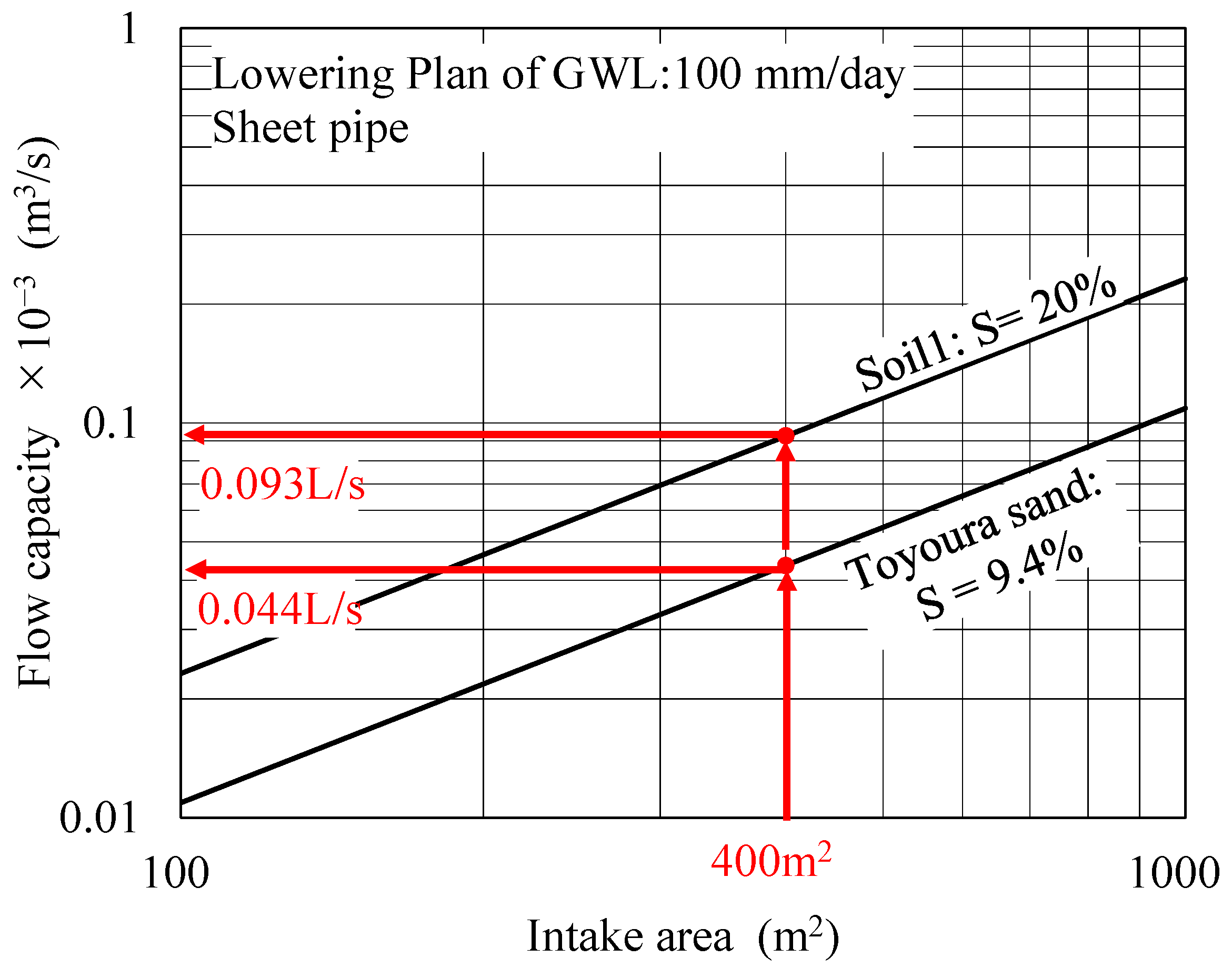
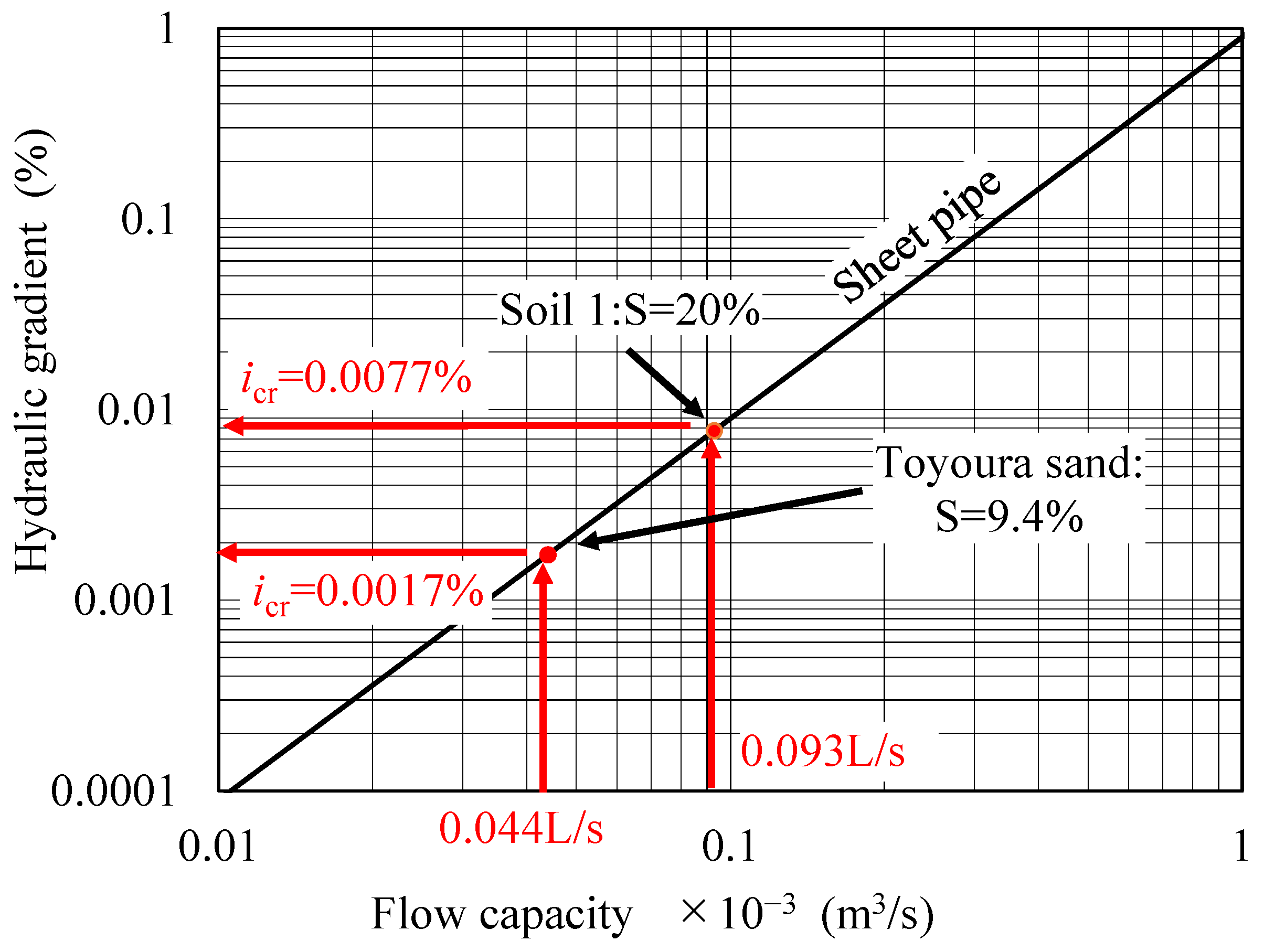
3.1. Flow Capacity of the Sheet Pipe

To compare the flow capacity of drainage pipes which are shown in Table 2, after placing the drainage pipe, a predetermined weight of Toyoura sand with a relative density Dr = 60% was poured into MT-MSB by the water pluviation method, and after initial settings of the data logging equipment, the drainage tests were started.
Figure 9 shows the relationships between the volume of water discharged from MT-MSB filled with only water and elapsed time. In the case of only mesh which is shown in Figure 8b, the volume of discharged water reaches 56 × 10−3 m3 at 100 s. For pipes C and D, tendencies of water accumulation are similar to those of only mesh filter. Although the accumulations of the water for A, B, and E are delayed, Pipe A and E reach the same level as Pipe C and D at 220 s.
Figure 10 shows the results for the case that the MT-MSB was filled with sand and water. For all pipes except for pipe B, the volume of discharged water reaches the same level at 600 min.
Based on the results as shown in Figure 10, the coefficient of flow capacity Cd which is defined as the ratio of the volume of discharged water through each drainage pipe to that through only the wire mesh filter was obtained. In Table 3, Cd for each drainage pipe is shown and it is seen that at the time of 600 min, Cd exceeds 90% for pipes A, C, D and E, and that at 1000 min, pipe A reaches 100%. In this research, since relatively high permeable soil compared with the farmland soil is used, the flow capacity of the sheet pipe is satisfied enough. This point is discussed later more in detail.
Figure 11 shows the change of flow capacity with the logarithm of elapsed time. At 10 s after opening the drainage valve, the flow capacity reaches 40 × 103 mm3/s and 26 × 103 mm3/s for only wire mesh filter and Pipe A, respectively.

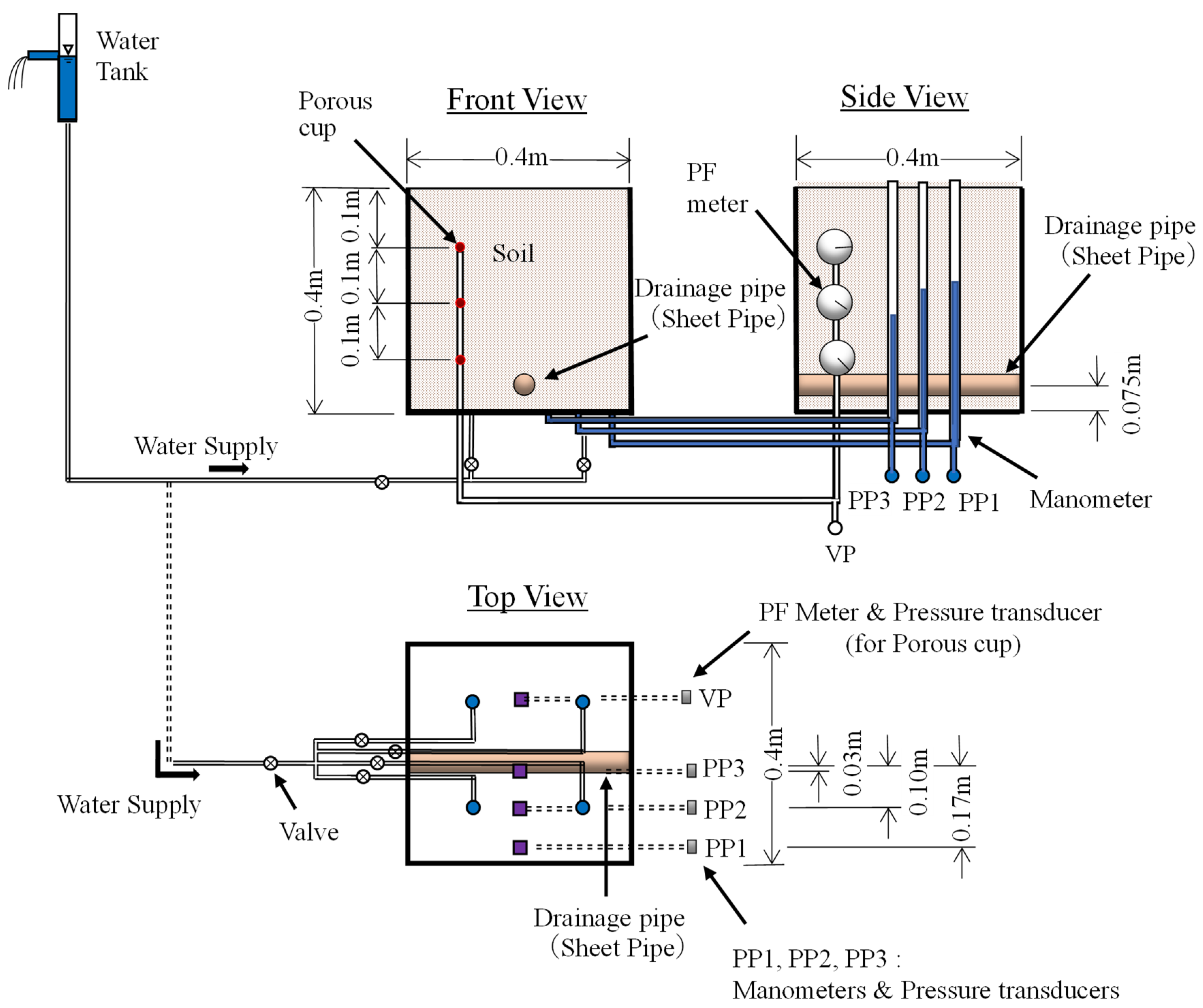
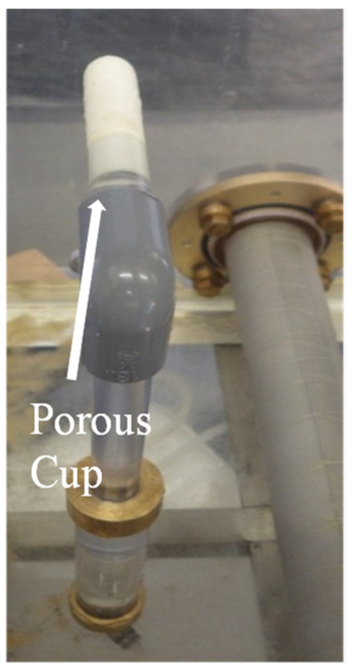
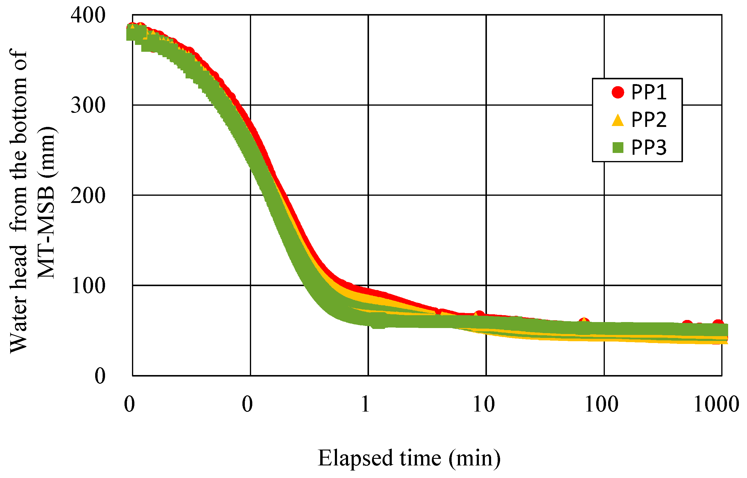
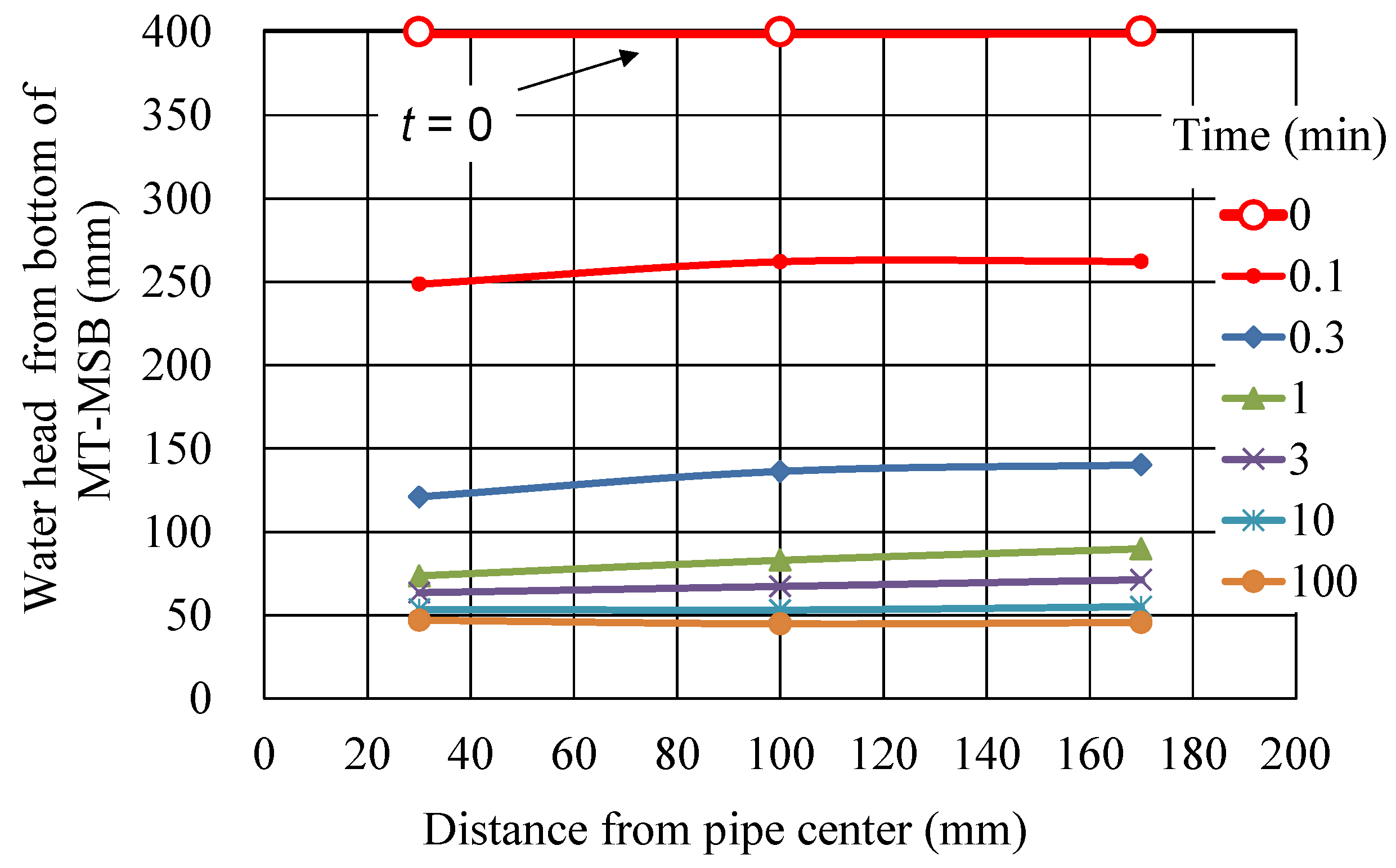
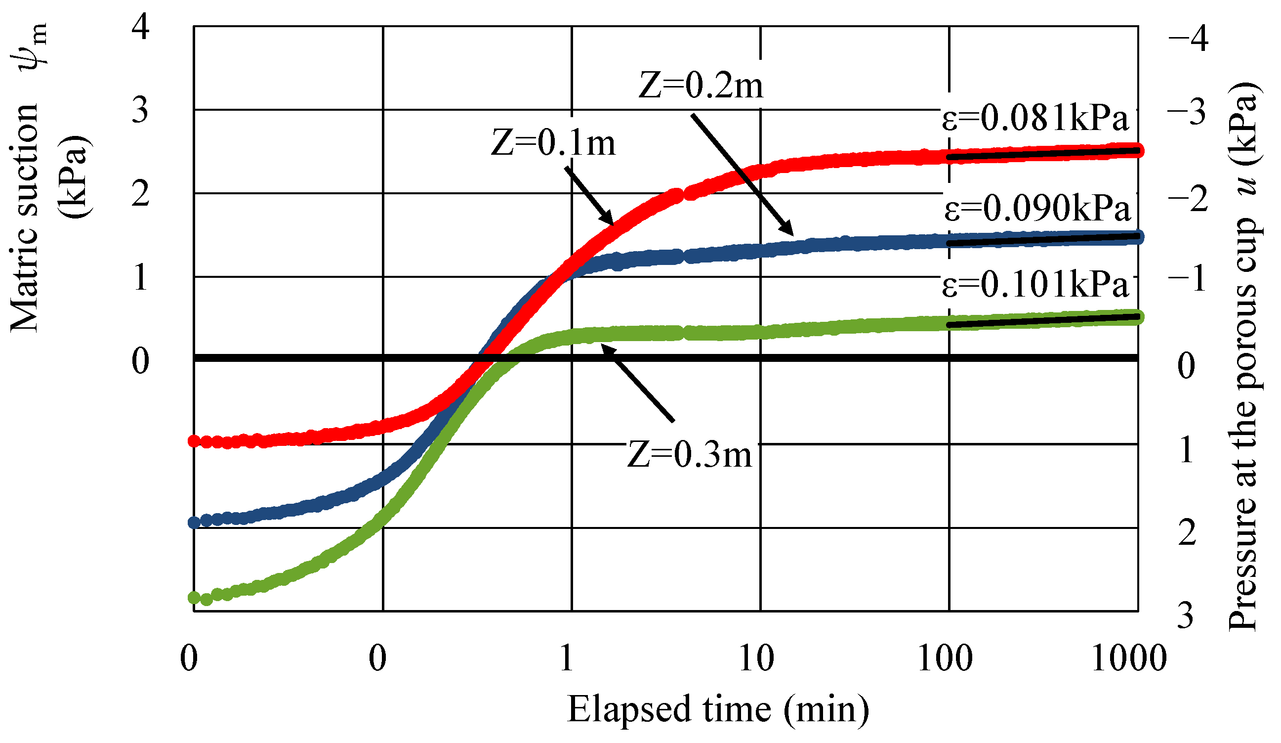
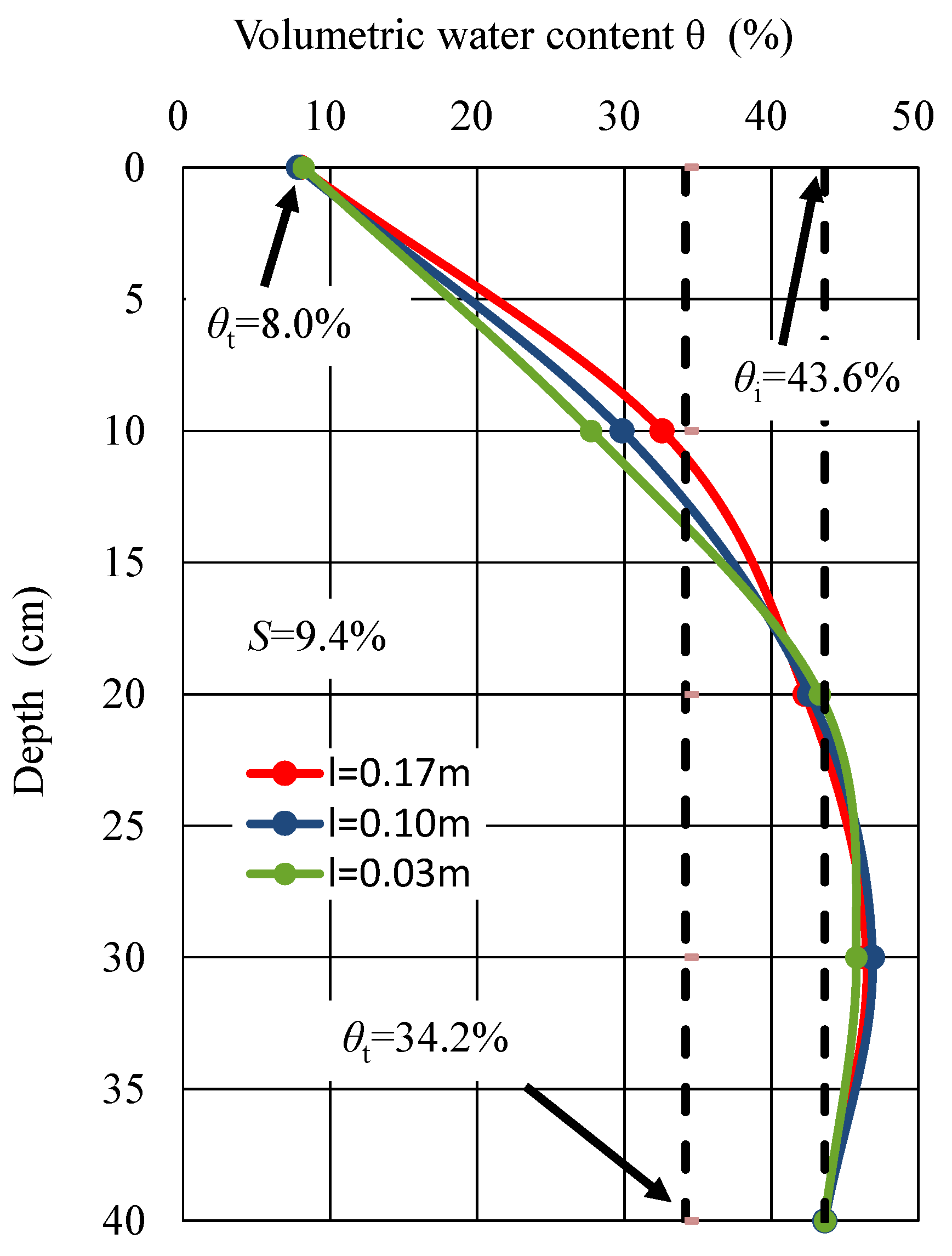
3.2. Effects of Drainage by the Sheet Pipe on the Water Head, Matric Suction, and Storage Coefficient

As mentioned before, hydraulic pressures at small holes PP1, PP2, and PP3 on the base plate of MT-MSB were transferred to the pressure transducers. Based on the measured hydraulic pressures, the water head hw for each point was obtained by hw = u/γw, where u is the hydraulic pressure and γw is the unit weight of water. In Figure 12, changes of the water head are shown against the logarithmic time. It is seen that the decrease in the water head at PP1 and PP2, whose positions from the center of sheet pipe are farther than PP3, is apparently delayed. In Figure 13, changes of the approximated phreatic surface estimated by the hydraulic pressures with time are shown in which t = 0 means the initial value. After starting the drainage test, it is seen that the water head quickly drops and the gradient of the phreatic surface changes with the distance from the center of the drainage pipe. The approximated phreatic surface is curved near the sheet pipe. This means that the assumption by Dupuit-Forchheimer provides feasible solutions in a form simpler than that obtainable by rigorous analysis [20]. The continuity equation of water flow has been applied to the saturated porous medium to show the profiles of water level and their changes with time [6].
In the drainage tests, the change of hydraulic pressure was also measured through the porous cup column which was set horizontally at the depth 0.10 m, 0.20 m, and 0.30 m from the top surface of MT-MSB by the pressure transducer with the pressure capacity from −100 kPa to100 kPa. Although the porous cup was placed at the depth Z = 0.1 m, 0.2 m or 0.3 m from the top surface of MT-MSB, for the precise measurement of the matric suction under the limited space in MT-MSB, the depth of the porous cup was set individually for each test. This means that a series of drainage tests under the same condition consists of three tests with the depth of porous cup as Z = 0.1 m, 0.2 m, and 0.3 m. Relationships between the hydraulic pressure u and logarithm of elapsed time are shown in Figure 14, in which the changes of matric suction ψm are also shown; ψm is the negative capillary pressure and defined as ψm = uau, where ua is the pore air pressure. When ua is assumed to be negligible, ψm = −u is obtained [21].
For every depth, it is seen that immediately after the start of drainage, the hydraulic pressure shows the hydrostatic pressure for each depth and decreases to zero after about 20 s. Thereafter, the hydraulic pressures show negative values, the matric suctions increase and after passing the bending point of the curve, the gradient of the curve ε which is defined as ε = S u / l o g t gradually decreases. For the time between 100 min and 1000 min, however, it is seen that ε is almost constant but increases with the depth [14]. As an influence of suction on the time-dependent compression behavior of fill material, matric suction can increase the compression stiffness [22]. This means that at the surface of wet farm land, by lowering the GWL the shear strength increases with time even after the GWL becomes constant.
Although results obtained in this study might be important, to clarify this point more in detail, further experiments are required. However, such experiments exceed our current research objectives.
After finishing the drainage test, the water contents were measured at the depths Z = 0.0 m, 0.1 m, 0.2 m and 0.3 m with the horizontal distance l = 0.03 m, 0.10 m, and 0.17 m from the center of the sheet pipe.
Figure 15 shows the distributions of the volumetric water content θ with the depth, where θ is derived from the water content as follows: θ = Vw/V = γd/γw × w, where Vw is volume of water, V is the volume of soil and water, γd is the dry unit weight of soil, γw is the unit weight of water, and w is the water content. At Z = 0.1 m, there is a tendency that the closer the sampling position to the sheet pipe, the lower the volumetric water content. At Z = 0.2 m and 0.3 m, however, θ is almost the same.
Two broken lines in Figure 15 show the initial distribution θi and the average value θt after drainage tests. At the beginning of the test, since the soil is saturated, θi is obtained as θi = γd/γw × e/Gs = 43.6%.
For the case of unconfined aquifer, the storage coefficient S is obtained as a change of the volumetric water content by the following equation [23], and for Figure 15, S = 9.4% was obtained.
S = | d θ | = | θ i θ t |

3.3. Drainage Capacity by the Sheet Pipe

3.3.1. Maximum Drainage Capacity through the Horizontally Installed Sheet Pipe

Based on the above-mentioned results, the drainage capacities by the sheet pipe are discussed. Figure 16 shows the intake model for the subsurface drainage by the sheet-pipe system, in which As is the intake area, W is the space of installed sheet pipe, L is the length of sheet pipe, Dp is the depth of sheet pipe installation, S is the storage coefficient, and z is the lowering plan of GWL.
The intake volume of water VA and the flow capacity Q are obtained as follows [14,24],
V A = A s × z × S
Q = v × A
v = ( 1 n ) × R ( 2 / 3 ) × i ( 1 / 2 )
where v is the flow rate and obtained by the Manning’s equation which is widely used to determine the flow capacity for the gravity flow, i is the hydraulic gradient, and A is the flow area inside the sheet pipe. When the pipe is fully filled with water, then A = ( π 4 ) × D 2 . D is diameter of the sheet pipe, and R is the hydraulic mean depth. R is obtained by R = A / P , where P is the wetted perimeter, and n is Manning’s n value. In this study, n = 0.010 was used for the sheet pipe, based on Figure 17 [25].
As mentioned before, since the sheet pipe is installed horizontally in the subsurface layer, a method to predict the maximum lowering rate of the ground water level was developed [14]. When considering that the pipe is fulfilled with water at the downstream end of the sheet pipe, then the hydraulic gradient is named as the critical hydraulic gradient of the sheet pipe icr and obtained from Equations (2)–(4) as follows.
i cr = [ Q / { ( 1 4 ) 5 3 × π × D 8 3 × ( 1 / n ) } ] 2
When the sheet pipe is laid horizontally in the subsurface layer, if the following equation is satisfied, the sheet pipe is supposed not to be fulfilled with the water. Here, imax is the maximum gradient of the pipe.
i cr     i m a x = D / L
Then the maximum flow capacity Qmax is given as follows.
Q m a x = ( 1 / 4 ) 5 / 3 × π × D 8 / 3 × ( 1 n ) × ( i m a x ) 1 / 2
When the storage coefficient S is obtained or predicted, the maximum lowering rate of GWL ∆zmax is obtained as,
z m a x = Q m a x / ( A s × S )
To confirm the applicability of this method, firstly the critical hydraulic gradient icr was calculated for the condition as ∆z = 100 mm/day, D = 50 mm, L = 100 m, W = 4.0 m, n = 0.010 and S = 9.4% which was obtained in the above-mentioned experiments on Toyoura sand. Figure 18 shows the results on the flow capacity of the sheet pipe for ∆z = 100 mm/day on Toyoura sand. In the same figure, a result for Soil1 which was obtained by the hollow-cylinder used drainage tests with 82.5 cmH and 5.2 cmD [23] is shown. For Toyoura sand (S = 9.4%) and Soil1 (S = 20.0%), as a flow capacity, 0.044 × 10 3 m 3 / s and 0.093 × 10 3 m 3 / s were obtained, respectively.
In Figure 19, the critical hydraulic gradient of the sheet pipe icr on two soils were obtained as icr = 0.0017% for Toyoura sand and icr = 0.0077% for Soil1 as follows.
i cr = 0.0017 % ,   0.0077 %   < <   50 100 , 000 = 0.05 %
It is apparent that these results satisfy Equation (6) and this means that even if the ground water level is lowered as ∆z = 100 mm/day, the sheet pipe would not be fulfilled with water.
Maximum flow capacity Qmax and maximum lowering rate of GWL ∆zmax are obtained by Equations (7) and (8) and results on two soils are summarized in Table 4. For the maximum flow capacity of the sheet pipe, Qmax = 0.237 × 10 3 m 3 / s was confirmed less than Q = 1.14 × 10 3 m 3 / s which was obtained at 10 s after starting in the direct drainage test through the sheet pipe in the MT-MSB without the soil and mesh filter.

3.3.2. Limitations and Constraints

The shape of the water table between parallel drain pipes is generally described as elliptical or the fourth-degree parabola [5,26]. In the above mentioned intake model, however, to find the drainage capacity of the sheet pipe, the ground water table was assumed to drop down keeping the water table horizontal as an average.
For these water tables, to find the drain spacing there are two types of formula commonly used. These are the steady state formula and the non-steady state formula. As a steady state formula, the Hooghoudt formula, and as a non-steady state formula, the Glover-Dumm drainage formula have both been used for determining the desirable spacing and depth of drains to maintain the water table below a certain level [20,26,27]. In these two types of formula, since the Glover-Dumm drainage formula is based on the schematization h < d< < W, the pipe spacing should be much larger than h and d, where h is the height of the ground water table at the midway point between drains and d is the equivalent depth to the impermeable substratum [26]. In this study, since the impermeable layer in the MT-MSB was placed at almost the same level as the drain and in the sheet pipe system, the drain spacing is set empirically as short as about 4 m, the Hooghoudt formula as shown below was used.
W 2 = 8 k 2 d h q + 4 k 1 h 2 q
where k1 and k2 are the hydraulic conductivity for the upper and lower layer, respectively, (m/d) and q is the discharge rate per unit horizontal area (m/d). Table 5 shows the results obtained by Equation (10) under the condition of the soil which is isotropic and homogeneous for the water flow. As for the thickness of equivalent layer below the drains was set as 0.7 m and the height of GWL at the center between drains was changed as 0.1, 0.2 m and 0.3 m. For these conditions, the spacing of the drainage pipe was obtained as 19.9 m, 15.8 m and 10.9 m, respectively. These drain spacings are larger than W = 4.0 m. This means that the maximum flow capacity obtained in this study is applicable as a safe side.

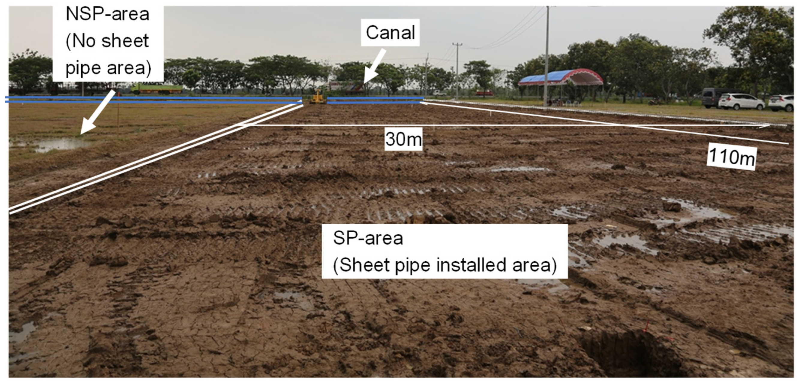
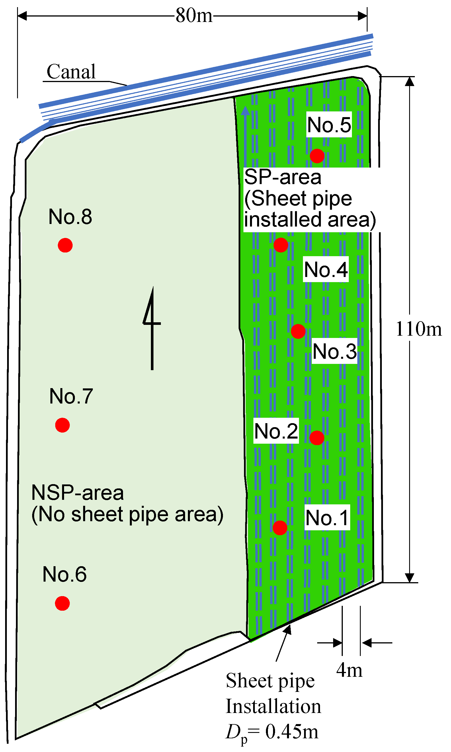
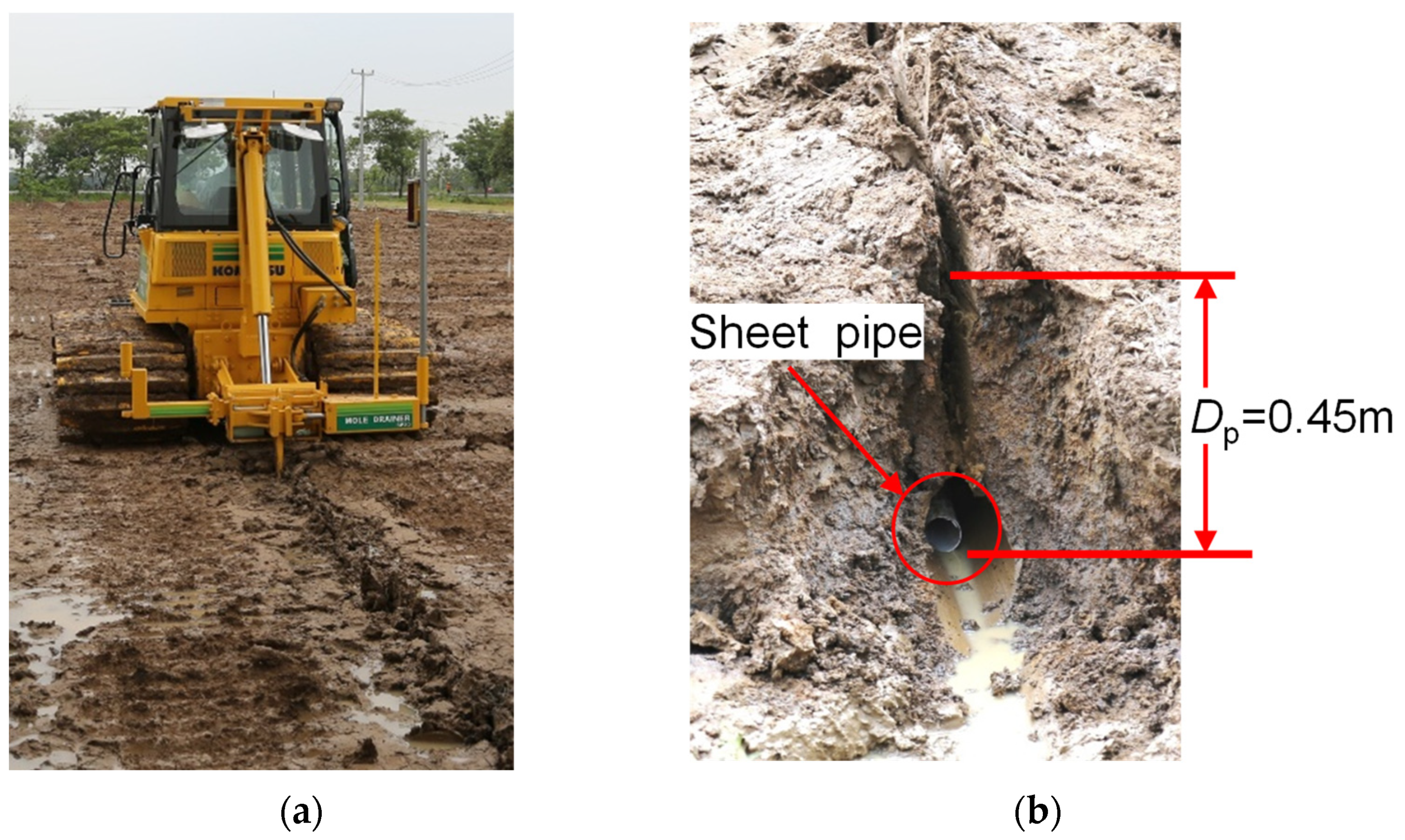
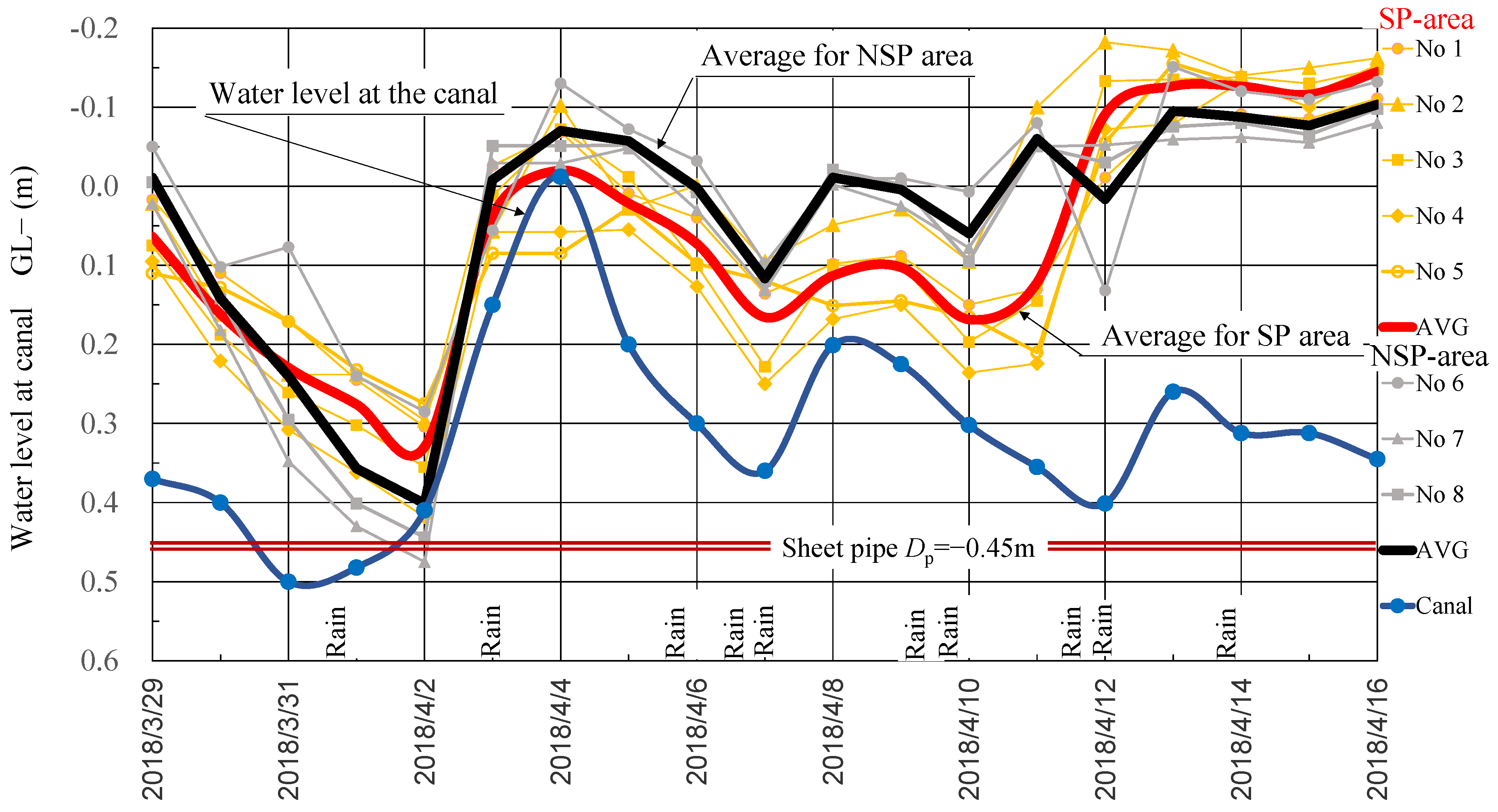
3.4. A Case Study on the Drainage by Using the Sheet-Pipe System

The first application of the sheet-pipe system was performed at the Indonesian Center for Rice Research, Sukamandi, West Java, Indonesia in 2018 as a pilot project [12,14]. The tested site is a paddy field with an area of 10,000 m2 and the field was divided into two areas (i.e., as a sheet pipe installed area (SP-area) and non sheet pipe area (NSP-area)). In SP-area, the sheet pipe was installed by the Mole Drainer at a depth of Dp = 0.45 m and the sheet pipe spacing was set as 4.0 m. The pilot project area and outline of the test field are shown in Figure 20 and Figure 21. Figure 22a shows a mole drainer which is drawing the sheet pipe into the paddy field and Figure 22b shows the cross section of the sheet pipe installed in the subsurface layer.
As shown in Figure 20 and Figure 21, a narrow canal is located at the north end of the test site into which the water was discharged through the sheet pipe. Table 6 shows the physical properties of samples obtained at Nos.1–5 in Figure 21 and the coefficients of permeability observed by the tube method. It is seen that all the soils are classified as CH (Inorganic clay with high plasticity) and the permeability is very low compared with the soil used in the MT-MSB tests as mentioned before.
At the SP-area, the sheet pipe was installed on 12 and 13 March, 2018. Figure 23 shows the changes of GWL observed at the bore holes in SP-area and NSP-area (red and black lines show the average of GWL for SP-area and NSP-area, respectively) and the water level at the canal.
In the same field, the evaluation of the sheet-pipe system on the crop productivity was conducted based on the field investigation from 5 May to 6 August, 2018 as one rice season. At the SP-area, the grain yield with more than 13.36% was confirmed [12].
When focusing on from 4 to 12 April, 2018 in Figure 23, GWL is affected by the sheet pipe used drainage, rain, and the water level at the canal. Especially, by quick dropping of the water level in the canal, definite differences in GWL between SP and NSP areas are seen, e.g., on 6 April, GWL at the SP area is 0.073 m and at the NSP area is 0.002 m, so GWL at the SP area is 0.071 m lower than the NSP area. This means that although GWL is affected by the rain and water level at the adjoining canal, even in such a case as that the free board in the canal is limited, the sheet pipe system functions effectively.
By applying Equation (10) to this site q is obtained for the parameters as the coefficient of permeability k1 = k2 = kav = 1.39 × 10⁻⁷ m/s, where kav is the average coefficient of permeability of those shown in Table 6 and the pipe spacing W = 4.0 m. Then since no information about the layer below the sheet pipe was obtained, the thickness of equivalent layer was set as d = 0.7 m. As a result, q = 1.5 mm/d, 0.96 mm/d and 0.45 mm/d for h = 0.3 m, 0.2 m, and 0.1 m were obtained, respectively. The average of daily drop of GWL measured at the site between 5 and 7 April is 93 mm, and this value is significantly larger than the calculated ones. The reasons why these differences occur are mainly considered due to that the available equations including the Equation (10) are based on assumptions such as isotropic and homogeneous of soil to idealize and simplify the flow system [15].

4. Conclusions

In this study, to clarify the applicability of the sheet-pipe system to a wet land which is affected easily by the ground water level rising, firstly, the differences in the flow capacity between the sheet pipe and another type of commercially used pipes were observed. Secondly, in the sheet-pipe system, when the sheet pipe is drawn horizontally into the subsurface layer where the free board of the adjoining canal is limited, the maximum lowering rate of the ground water level was derived based on the storage coefficient obtained by MT-MSB tests. Thirdly, as a case study, the sheet pipes were laid at the level farm land close to the canal. The efficiencies of the sheet-pipe system were confirmed by comparing the change of the ground water level at the farmland with a sheet pipe and without one (concerning the rain, water level at the adjoining canal, drainage capacity of the sheet pipe, and the pipe spacing).
These results mean that at a wet farmland such as one near the seacoast with a relatively smaller block in area, subsurface drainage is possible and the sheet-pipe system would especially contribute to the sustainable restoration of degraded farm land due to climate change-induced rise of GWL or salinization.
When spreading the subsurface drainage at a wetland, as an advantage, the agricultural mechanization might develop further by the improvement of trafficability due to the suction-induced increase of the bearing capacity at the ground surface.

Author Contributions

Conceptualization and methodology, K.T., H.M.; writing—review and editing, K.T., H.M., B.I.S. and S.K.S.; funding acquisition, K.T. All authors have read and agreed to the published version of the manuscript.

Funding

This research was partly funded by Japan International Cooperation Agency.

Data Availability Statement

The data presented in this research are available on request from the corresponding author. The data are not publicly opened since the ownership is shared by all members who contributed to this research.

Acknowledgments

This research was supported by Japan International Cooperation Agency, Yamaguchi University, and the Indonesia Center for Rice Research in the case studies. The authors would like to express their gratitude to them.

Conflicts of Interest

The authors declare no conflict of interest.

References

  1. Vineis, P.; Chan, Q.; Khan, A. Climate change impacts on water salinity and health. J. Epidemiol. Glob. Health 2011, 1, 5–10. [Google Scholar] [CrossRef] [PubMed] [Green Version]
  2. Ullah, A.; Bano, A.; Khan, N. Climate change and salinity effects on crops and chemical communication between plants and plant growth-promoting microorganisms under stress. Front. Sustain. Food Syst. 2021, 5, 1–16. [Google Scholar] [CrossRef]
  3. Kang, N.; Kim, S.; Kim, Y.; Noh, H.; Hong, S.J.; Kim, H.S. Urban drainage system improvement for climate change adaptation. Water 2016, 8, 268. [Google Scholar] [CrossRef] [Green Version]
  4. Fukuda, T.; Shinogi, Y. Drainage mechanism of sheet pipe underdrainage and desalination effect. Jpn. Soc. Irrig. Drain. Rural. Eng. 2015, 83, 326–327. (In Japanese) [Google Scholar]
  5. Hillel, D. 8 Groundwater Drainage. In Soil and Water; Academic Press: New York, NY, USA, 1971; pp. 167–181. [Google Scholar]
  6. Setiawan, B.I.; Arif, C.; Saptomo, S.K.; Matsuda, H.; Tamura, K.; Inoue, Y. Water Flow in Soils Installed with Sheet-Pipe Model Drains; PAWEES (International Society of Paddy and Water Environment Engineering): Nara, Japan, 2018; pp. 743–748. [Google Scholar]
  7. Sugiyama, M.; Tsuda, Y. Construction method on the cross culvert by sheet pipe and the condition after construction. JSIDRE J. 1990, 58, 159–167. (In Japanese) [Google Scholar]
  8. Soe, Y.M.; Shinogi, Y.; Taniguchi, T. Impacts of perforated sheet pipe installation on some paddy soil properties. Paddy Water Environ. 2019, 17, 151–164. [Google Scholar] [CrossRef]
  9. Sasmita, P.; Agustiani, N.; Margaret, S.; Yusup, A.M.; Tamura, K. The effect of sheet-pipe technology application on soil properties, rice growth, yield and prospect to increase planting index. In Proceedings of the 1st International Conference on Sustainable Tropical Land Management, Virtual Conference, 16–18 September 2020; Volume 648, pp. 1–9. [Google Scholar]
  10. Arif, C.; Setiawan, B.I.; Saptomo, S.K.; Matsuda, H.; Tamura, K.; Inoue, Y.; Hikmah, Z.M.; Nugroho, N.; Agustiani, N. Water use efficiency and productivity in paddy field under subsurface drainage technology with sheet-pipe system. In Proceedings of the 3rd World Irrigation Forum (WIF3), Bali, Indonesia, 1–7 September 2019; pp. 1–10. [Google Scholar]
  11. Setiawan, B.I.; Saptomo, S.K.; Arif, C.; Matsuda, H.; Tamura, K.; Inoue, Y. Automatic subsurface irrigation and drainage using sheet-pipe typed model drain. In Proceedings of the 3rd World Irrigation Forum (WIF3), Bali, Indonesia, 1–7 September 2019; pp. 1–11. [Google Scholar]
  12. Arif, C.; Setiawan, B.I.; Saptomo, S.K.; Matsuda, H.; Tamura, K.; Inoue, Y.; Hikmah, Z.M.; Nugroho, N.; Agustiani, N.; Suwarno, W.B. Performances of sheet-pipe typed subsurface drainage on land and water productivity of paddy fields in Indonesia. Water 2021, 13, 48. [Google Scholar] [CrossRef]
  13. Agriculture Victoria. Available online: https://agriculture.vic.gov.au/livestock-and-animals/dairy/managing-wet-soils/types-of-subsurface-drainage-systems#h2-1 (accessed on 18 September 2021).
  14. Matsuda, H.; Tamura, K.; Setiawan, B.I.; Saptomo, S.K. Effects of drainage by the sheet pipe on the suction and volume water content of subsurface layer. In Proceedings of the XVII European Conference on Soil Mechanics and Geotechnical Engineering, Reykjavik, Iceland, 1–6 September 2019; pp. 1–9. [Google Scholar]
  15. Hillel, D. Introduction to Environmental Soil Physics; Elsevier Academic Press: Cambridge, MA, USA, 2004; p. 327. [Google Scholar]
  16. Verdugo, R.; Ishihara, K. The steady state of sandy soils. Soils Found. 1996, 36, 81–91. [Google Scholar] [CrossRef] [Green Version]
  17. Zhang, F.; Jin, Y.; Ye, B. A try to give a unified description of Toyoura sand. Soils Found. 2010, 50, 679–693. [Google Scholar] [CrossRef] [Green Version]
  18. Koseki, J.; Yoshida, T.; Sato, T. Liquefaction properties of Toyoura sand in cyclic tortional shear tests under low confining stress. Soils Found. 2005, 45, 103–113. [Google Scholar] [CrossRef] [Green Version]
  19. Kato, S.; Ishihara, K.; Towhata, I. Undrained shear characteristics of saturated sand under anisotropic consolidation. Soils Found. 2001, 41, 1–22. [Google Scholar] [CrossRef] [Green Version]
  20. Hillel, D. Environmental Soil Physics; Academic Press: Cambridge, MA, USA, 1998; p. 485. [Google Scholar]
  21. Zhang, C.; Lu, N. Unitary definition of matric suction. J. Geotech. Geoenviron. Eng. ASCE 2019, 145, 1. [Google Scholar] [CrossRef]
  22. Chen, W.B.; Liu, K.; Feng, W.Q.; Borana, L.; Yin, J.H. Influence of matric suction on nonlinear time-dependent compression behavior of a granular fill material. Acta Geotech. 2020, 15, 615–633. [Google Scholar] [CrossRef]
  23. Mogami, T. Seepage, 3rd ed.; Kajima Institute Publishing Co., Ltd.: Tokyo, Japan, 1979; p. 19. (In Japanese) [Google Scholar]
  24. Kikuoka, T. Handbook on Irrigation, Drainage and Reclamation Engineering; Maruzen Publishing: Tokyo, Japan, 1979; p. 790. (In Japanese) [Google Scholar]
  25. Suetsugu, Y.; Yamanaka, H. Technical Reports of Shin-Etsu Sheet Pipe; Shin-Etsu Polymer Co. Ltd.: Saitama, Japan, 2003. (In Japanese) [Google Scholar]
  26. Vlotman, W.F.; Smedema, L.K.; Rycroft, D.W. 11 Design of pipe drainage systems. In Modern Land Drainage; CRC Press: London, UK, 2020; pp. 195–225. [Google Scholar]
  27. Raadsma, S. 7 Current Draining Practices in Flat Areas of Humid Regions in Europe. In Drainage for Agriculture; Dinaure, R.C., Davis, M.E., Eds.; American Society of Agronomy, Inc.: Madison, WI, USA, 1974; p. 132. [Google Scholar]
Figure 1. (a) Rolled-band sheet (100 m in length) with the perforated drainage holes, (b) sheet pipe transformed from the rolled-band sheet.
Land 10 01328 g001
Figure 2. Process of insertion of the sheet pipe into the subsurface layer.
Land 10 01328 g002
Figure 3. Outline of the miniature-type model soil box (MT-MSB).
Land 10 01328 g003
Figure 4. Setup of the porous cup.
Land 10 01328 g004
Figure 5. MT-MSB filled with sand and water.
Land 10 01328 g005
Figure 6. Particle size distribution curve.
Land 10 01328 g006
Figure 7. Wire mesh filter.
Land 10 01328 g007
Figure 8. Setup of wire mesh filter in MT-MSB.
Land 10 01328 g008
Figure 9. Drainage from MT-MSB filled with only water.
Land 10 01328 g009
Figure 10. Drainage from MT-MSB filled with water and sand.
Land 10 01328 g010
Figure 11. Change of flow rate with elapsed time.
Land 10 01328 g011
Figure 12. Changes of water head by drainage through the sheet pipe.
Land 10 01328 g012
Figure 13. Distribution of water head.
Land 10 01328 g013
Figure 14. Change of the matric suction.
Land 10 01328 g014
Figure 15. Distributions of volumetric water content.
Land 10 01328 g015
Figure 16. Intake model by the sheet-pipe system.
Land 10 01328 g016
Figure 17. Manning’s n value for the sheet pipe [25].
Land 10 01328 g017
Figure 18. Flow capacity of the sheet pipe.
Land 10 01328 g018
Figure 19. Critical hydraulic gradient.
Land 10 01328 g019
Figure 20. Pilot project area of 1000 m2.
Land 10 01328 g020
Figure 21. Outline of the test site.
Land 10 01328 g021
Figure 22. (a) Sheet pipe is under drawn into the ground, (b) cross section of subsurface layer after the insertion of sheet pipe.
Land 10 01328 g022
Figure 23. Effect of sheet pipe drainage on the ground water level lowering at the test site.
Land 10 01328 g023
Table 1. Physical properties of sample.
ρs (g/cm3)2.673
emax0.991
emin0.630
k (m/s) Dr = 60%2.246 × 10⁻⁴
k (m/s) Dr = 70%1.700 × 10⁻⁴
k (m/s) Dr = 80%1.629 × 10⁻⁴
Table 2. Dimensions of typical drainage pipes.
Drainage PipeDiameter (mm)Drainage Hole Size (mm)Thickness (mm)Length (mm)
A (Sheet pipe)50.5φ21.0400.0
B60.0φ74.1400.0
C59.68 × 15.0400.0
D60.4--400.0
E54.0φ72.0400.0
Table 3. Coefficients of drainage capacity for each drainage pipe.
Time (min)Coefficient of Drainage Capacity
Pipe APipe BPipe CPipe DPipe E
2000.790.630.850.950.93
3000.830.650.870.940.92
4000.860.670.880.940.92
5000.890.680.890.930.91
6000.920.690.910.930.91
7000.940.690.920.930.91
8000.970.70.930.930.91
9000.980.70.950.940.92
100010.710.970.940.92
Table 4. Maximum drainage capacity Qmax and maximum lowering rate of GWL.
SampleS (%)L (m)W (m)D (mm)Δz (mm/d)Q (×10−3) (m3/s)i (%)Qmax (×10−3) (m3/s)Δzmax (mm/d)
Toyoura sand9.4100.04.050.0100.00.0440.0170.237543.4
Soil120.0100.04.050.0100.00.0930.0770.237255.4
Table 5. Pipe spaces calculated by Hooghoundt’s equation.
Sample Toyoura Sand
h (height of GWL at the center above pipe) m0.300.200.10
ΔZ = q (lowing rate of GWL) m/d0.100.100.10
W (drain spacing) m19.9015.7610.79
Note: Relative density Dr = 60%. Coefficient of permeability for above and below drainage pipe k1 = k2 = 2.246 × 10−4 = m/s. Thickness of equivalent Layer d = 0.7 m.
Table 6. Physical properties of sample at SP-area (0.0–0.5 m).
Bore HoleNo.1No.2No.3No.4No.5
Clay(%)
<0.005 mm
69.1080.7567.0661.8257.77
Silt(%)
<0.075 mm
29.7619.2529.7236.0239.43
Fine sand(%)
<0.420 m
1.140.003.002.162.12
w (%)29.8537.4536.1439.5234.37
Gs2.5402.5352.5442.5312.493
PI32.7745.3744.1832.9737.80
Void ratio0.760.960.931.010.87
k (m/s)3.75 × 10−81.98 × 10−71.47 × 10−75.9 × 10−93.09 × 10⁻⁷
Note: w, water content; Gs, specific gravity; PI, plasticity index; k, coefficient of permeability.
Publisher’s Note: MDPI stays neutral with regard to jurisdictional claims in published maps and institutional affiliations.

