Article

Evaluating the Effect of Deforestation on Decadal Runoffs in Malaysia Using the Revised Curve Number Rainfall Runoff Approach

1
Centre of Disaster Risk Reduction (CDRR), Lee Kong Chian Faculty of Engineering & Science, Universiti Tunku Abdul Rahman, Jalan Sungai Long, Kajang 43000, Malaysia
2
Centre for Photonics and Advanced Materials Research, Lee Kong Chian Faculty of Engineering & Science, Universiti Tunku Abdul Rahman, Jalan Sungai Long, Kajang 43000, Malaysia
*
Author to whom correspondence should be addressed.
Water 2023, 15(7), 1392; https://doi.org/10.3390/w15071392
Submission received: 14 March 2023 / Revised: 23 March 2023 / Accepted: 27 March 2023 / Published: 4 April 2023

Abstract

:
This study presents a revised and calibrated Soil Conservation Service (SCS) curve number (CN) rainfall runoff model for predicting runoff in Malaysia using a new power correlation Ia = SL, where L represents the initial abstraction coefficient ratio. The traditional SCS-CN model with the proposed relation Ia = 0.2S is found to be unreliable, and the revised model exhibits improved accuracy. The study emphasizes the need to design flood control infrastructure based on the maximum estimated runoff amount to avoid underestimation of the runoff volume. If the flood control infrastructure is designed based on the optimum CN0.2 values, it could lead to an underestimation of the runoff volume of 50,100 m3 per 1 km2 catchment area in Malaysia. The forest areas reduced by 25% in Peninsular Malaysia from the 1970s to the 1990s and 9% in East Malaysia from the 1980s to the 2010s, which was accompanied by an increase in decadal runoff difference, with the most significant rises of 108% in Peninsular Malaysia from the 1970s to the 1990s and 32% in East Malaysia from the 1980s to the 2010s. This study recommends taking land use changes into account during flood prevention planning to effectively address flood issues. Overall, the findings of this study have significant implications for flood prevention and land use management in Malaysia. The revised model presents a viable alternative to the conventional SCS-CN model, with a focus on estimating the maximum runoff amount and accounting for land use alterations in flood prevention planning. This approach has the potential to enhance flood management in the region.

1. Introduction

Water is crucial for supporting life and economic development, but it is a scarce resource. Freshwater accounts for only 2.5% of the water on Earth, which is suitable for basic human needs such as drinking, cooking, and bathing. The scarcity of water is a result of the disparity between its supply and demand. Research on effective water resource management is essential, and it is also a practical subject. However, water-related disasters such as floods and droughts can result in the loss of life and property, making it difficult to manage water resources effectively [1].
The analysis of extreme hydrometeorological events is crucial in characterizing and comprehending the meteorological conditions that cause severe rainstorms and subsequent devastating floods. The situation becomes worse when these extreme events overlap. Compound extremes pose significant challenges and dangers to communities, especially when they involve hydrometeorological events such as floods, surges, droughts, and heatwaves that can be deadly. To better mitigate and adapt to these compound hydrometeorological extremes, it is necessary to have a better understanding of these events and their potential occurrence. The detection of trends in hydroclimatic variables such as temperature, precipitation, and streamflow plays a significant role in understanding the variations and changes in the climate. It is essential to comprehend the connections between the trends in climate fluctuations and extreme hydrometeorological events in order to plan for water and agricultural management and anticipate the dangers associated with these events [2,3,4,5].
Flooding is a destructive occurrence that happens when water overflows onto land and rises above its typical level, usually due to excessive rainfall that cannot be absorbed by the soil, which results in runoff. When the volume of runoff surpasses the capacity of available flood control infrastructure, water overflows and causes flooding. These events can have severe consequences for individuals and countries alike, as they threaten lives, especially of those living in low-lying areas, and result in significant financial losses from infrastructure damage and recovery efforts. To mitigate these impacts, it is crucial to understand the relationship between rainfall and runoff, which will improve the accuracy of runoff estimates and help the government better plan for flood management. For example, by having precise and reliable rainfall runoff models, governments can ensure the construction of adequate flood control systems, such as retention ponds and drainage systems, which will help reduce the risk of future floods [6,7].
Over the past few decades, a significant amount of research activities have been focused on the analysis and modelling of rainfall runoff, leading to the development of various types of models. The main objective is to predict the occurrence of floods in advance and prevent the associated losses. Hydrologic analysis and design rely heavily on the central aspect of rainfall runoff modelling, which depicts the interconnected surface and subsurface processes within a watershed. The importance of rainfall runoff modelling extends beyond hydrology and water resource management, as it aids in planning for watershed water resources, managing reservoirs, and preparing for drought and potential flood hazard events. Additionally, it provides insights into catchment yields and responses, water availability, and changes over time, making it a fundamental issue in watershed hydrology modelling and research [8,9,10,11].
Given the non-linear nature of the process, accurate simulations of the rainfall runoff process are crucial in hydrology and water resources management, and are highly dependent on the inputs to the simulation model. Despite the complexity associated with the transformation of rainfall into runoff, runoff analysis is crucial in predicting natural disasters such as floods and droughts. Furthermore, it plays a crucial role in the design and operation of water resource projects such as barrages, dams, and water supply schemes, and is necessary for water resources planning, development, and flood mitigation efforts [8,9,10,11].
The curve number (CN) model (Equation (1)) was created in 1954 by the United States Department of Agriculture (USDA) and Soil Conservation Services (SCS) to study rainfall and runoff using limited data from less than 200 catchments in the USA.
Q = P I a 2 P I a + S
where P = rainfall depth (mm), Q = runoff depth (mm), S = catchment maximum potential water retention (mm), and Ia = amount of initial abstraction (mm).
The SCS proposed the initial abstraction coefficient ratio (λ) relationship, Ia = λS, but the equation was weakly supported by data available at the time. To simplify calculations, the SCS set a constant value of 0.2 for λ in the equation (Figure 1), which became the conventional SCS-CN rainfall runoff prediction model (Equation (2)) [12,13,14,15].
Q = P 0.2 S 2   P + 0.8 S
where the restriction of P > 0.2S (or Ia < P) must be obeyed, else there will be no runoff (Q) occurring.
The widely used CN runoff model was not specifically designed for many applications, yet is cited in hydrological manuals and incorporated into software. The accuracy and reliability of the model are important for related software and handbooks [16,17,18,19,20,21]. Researchers from various countries have challenged the use of a fixed value of 0.2 for the initial abstraction coefficient ratio (λ) in the equation Ia = λS, suggesting different ranges for λ that vary by region [22,23,24]. Using a fixed value of 0.2 can lead to inaccurate predictions of runoff amounts. Over 60 years, studies have aimed to find the optimal λ value to improve the model’s accuracy and reliability, but none have re-evaluated the relationship between Ia and S. The conventional model uses a linear correlation of Ia = 0.2S, which, if different, could change the entire model and require re-evaluation and re-derivation.
Urban flooding is a growing issue, causing loss of life, economic losses, and extensive destruction. Floods are the most frequent natural disaster globally, with climate change increasing rainfall frequency and intensity. Urbanization and construction activities lead to increased impervious surfaces, limiting natural infiltration and evapotranspiration and converting rainfall into runoff. These factors, along with human resource demands on water quality and quantity, have led to harmful ecological and economic impacts on catchment water resources. Climate change, human activities, and land use changes impact the amount of surface water flow, known as runoff depth, with urbanization having a negative impact, and land conversion to grass or forest having a positive impact. Changes in vegetation and forest area can also significantly impact the runoff regime [25,26,27,28,29,30,31,32,33].
Based on previous studies, the linear correlation model of Ia = 0.2S proposed by the SCS was not statistically significant using the original data from 1954. Instead, the best linear models found were Ia = 0.112S [34] and Ia = 0.111S [35]. Thus, it is crucial to reassess the recalibration of the SCS-CN rainfall runoff model before using it, given the discreditation of the linear correlation of Ia = 0.2S.
In this paper, the SCS-CN rainfall runoff model was revised and calibrated using the power correlation Ia = SL, which has previously been explored by the authors in a separate study [12], to predict runoff in Peninsular Malaysia and East Malaysia. The results of this study demonstrate the potential for the newly calibrated power regressed model to be used to model decadal rainfall runoff conditions in Malaysia. Additionally, the study established a correlation between deforestation and urbanization on runoff increment in both Peninsular Malaysia and East Malaysia.

2. Materials and Methods

2.1. New Power Correlation of Ia = SL

To date, no research has been conducted to calibrate the SCS-CN model using a nonlinear correlation between Ia and S. Therefore, this study re-evaluates the runoff prediction ability of the conventional SCS-CN rainfall runoff model (Equation (2)) against the newly derived SCS model using a power correlation equation (Ia = SL) to simplify the fundamental SCS model (Equation (1)) and calibrate it using local rainfall runoff datasets with statistical methods. The newly formulated runoff predictive model will only have two fitting parameters, namely S and L, to maintain its parsimonious form as SCS fundamental Equation (1). The proposed parameter L is also a dimensionless parameter similar to SCS’s λ.
The previous SCS conventional rainfall runoff model, Equation (2), was simplified with Ia = 0.2S. However, past studies found Equation (2) to be insignificant at the α = 0.01 level, making it necessary to re-derive the model to improve the accuracy of its runoff predictions [34,35].

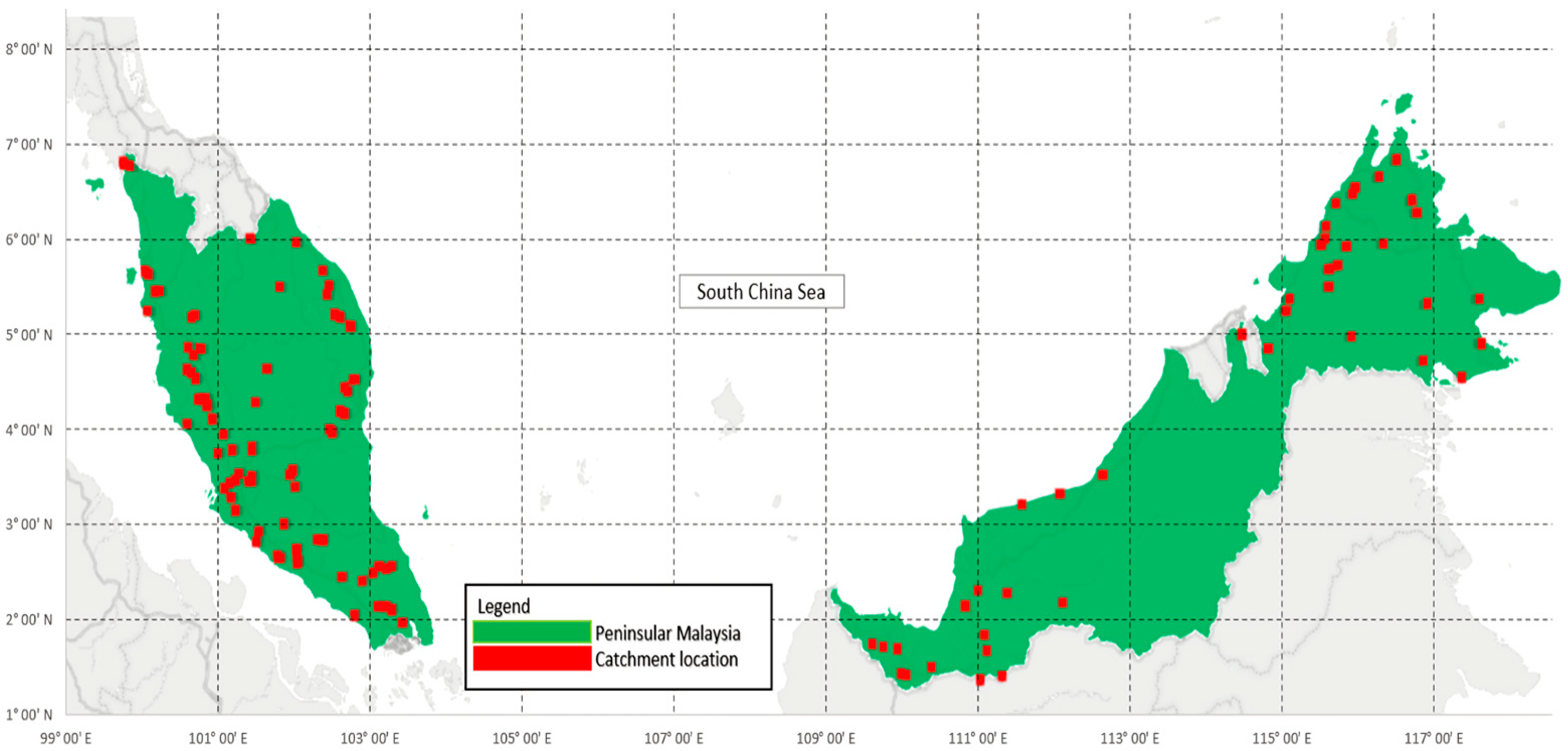
2.2. Study Sites in Malaysia

This study utilized data collected by the Department of Irrigation and Drainage (DID), a Malaysian federal agency. DID’s Hydrological Procedure no. 11 (DID-HP 11) gathered 474 pairs of rainfall runoff data from watersheds across Malaysia from 1964 to 2016, while DID’s Hydrological Procedure no. 27 (DID-HP 27) collected 227 pairs of rainfall runoff data from 1970 to 2000 [36,37]. The study combined both datasets, resulting in a total of 701 rainfall runoff datasets (rainfall range: 7–575 mm) collected from 1964 to 2016 for analysis. Thus far, this study has utilized the most extensive and up-to-date compilation of rainfall runoff data provided by the Malaysian federal agency, which encompasses a wide range of rainfall amounts. Figure 2 shows the catchment areas in Malaysia.

2.3. Decadal Analysis of Rainfall Runoff Models in Malaysia

In this study, decadal rainfall runoff analyses were conducted. The analysis covered Peninsular Malaysia and East Malaysia. For Peninsular Malaysia, data from 1970 to 2000 were divided into three decadal models: 1970s (70PM), 1980s (80PM), and 1990s (90PM). For East Malaysia, data from 1985 to 2016 were divided into three decadal models: 1985–1989 (85EM), 1990–1999 (90EM), and 2000–2016 (2KEM). After dividing the data into decade models, a decadal analysis was conducted to compare and analyze the trends in runoff conditions in Malaysia during each decade with the help of inferential statistics.
This study used statistical analysis to determine the optimal values of S and L for each decadal group. The bootstrapping method with the bias corrected and accelerated (BCa) procedure was conducted with 2000 random sampling (with replacement) at alpha = 0.01 through International Business Machine Corporation’s (IBM)’s Statistical Packages for Social Sciences (SPSS, version 21.0) statistical software to determine the total abstraction value (S), dimensionless initial abstraction ratio coefficient (L), and generated respective 99% confidence intervals (CI) for S and L. These results were then utilized to formulate a new SCS-CN rainfall runoff model and for the calculation of the CN value. The normality of the datasets was tested using the Kolmogorov–Smirnov and Shapiro–Wilk tests to determine whether the mean or median confidence intervals should be chosen for optimizing S and L for each dataset [38]. The Shapiro–Wilk test was given priority as it was more significant for sample sizes less than 2000, and all datasets in this study had a sample size of less than 2000. If the Shapiro–Wilk and Kolmogorov–Smirnov tests had a p-value of less than 0.05, it indicated that the datasets were not normally distributed, and the median CI was used for variable optimization, and vice versa [38].
The data distribution free bootstrap BCa technique was used in this study due to its robustness for analyzing rainfall runoff data [39,40,41]. Furthermore, the analytical module for bootstrap BCa is readily available in the IBM SPSS statistical software, making it a convenient choice for conducting the analysis needed in this study. The BCa method has the benefit of correcting biases and being able to produce the confidence interval of a particular variable at a selected significance level, which is very useful for further statistical analysis [39,40,41,42].
The calibration of the SCS runoff model was aimed to have zero bias in its overall prediction results by using a supervised numerical algorithm to find the best values of L and S that fulfilled the zero bias optimization constraint, within the 99% confidence interval of the bootstrap BCa. If zero bias optimization could not be achieved within the confidence interval, the optimization was set to maximize the Nash–Sutcliffe index (E). The accuracy and performance of the models were evaluated for each dataset based on the Nash–Sutcliffe index (E).
This study employs the Nash–Sutcliffe index (E), bias, and the Kling–Gupta efficiency (KGE) index to assess the predictive performance of the models. Equations (3)–(5) were used to calculate the E, bias, and KGE, respectively [12,43,44,45,46].
E = 1 i = 1 n Q predicted Q observed 2 i = 1 n Q predicted Q mean 2
BIAS = i = 1 n Q predicted Q observed   n
KGE = 1 r 1 2 + σ sim σ obs 1 2 + μ sim μ obs 1 2
where σ sim = the modelling results’ standard deviation, σ obs = the observed dataset’s standard deviation, μ sim = average of modelling results, μ obs = average of observed dataset, and r = correlation between modelling results and observed dataset.
In earlier research, the general formula for S was derived from Equation (1), which allowed for the computation of S through a closed form equation based on the P and Q data pairs [23,24,47,48]. To date, the power model Ia = SL substitution into Equation (1) in this study did not produce any closed form equation for S. Therefore, a numerical analysis technique is the only way to determine the value of S. The simplified formula for S is given in Equation (6) (the steps to derive and simplify the general formula for S based on the power regression model are outlined in Appendix A).
( 2 S L + Q 2 P ) 2 = 4 SQ + Q 2
The numerical analysis technique was used to find the optimum values of L and S (denoted as SL), according to the P and Q data pairs in this study by applying Equation (6). On the other hand, the S0.2 values for each data pair were also calculated using the general equation for S (Appendix B and shown in Equation (7)) [22,23,24,34,35,47,48,49] for curve number calculation.
S 0.2 = 5 P + 2 Q 4 Q 2 + 5 PQ  
The SL and S0.2 values were calculated separately according to the P and Q data pairs using Equations (6) and (7). The SPSS regression module was utilized to find the best correlation between SL and S0.2 datasets and determine the best correlation equation for the study site. This was done to examine the relationship between SL and S0.2 and convert SL back to its equivalent S0.2 value to obtain the conventional SCS curve number (CN0.2), which is commonly used by SCS practitioners. This correlation technique was introduced in [48]. The objective was to find the strongest correlation between SL and S0.2, with the highest adjusted R-squared value (R2adj), using SPSS statistical software [48,50,51] (the process is summarized in Appendix C). For example, the best correlation equation from SPSS between SL and S0.2 for the 1970s dataset in Peninsular Malaysia (modeled as 70PM) was identified in SPSS as:
S0.2 = (S0.168) 0.851
As introduced by the SCS, the equation to calculate the SCS curve number value is
CN 0.2 = 25,400 254 + S 0.2
where CN0.2 = the conventional curve number when λ = 0.2 and S0.2 = the total abstraction amount (mm) when λ = 0.2.
Equation (9) can also be expressed as Equation (10).
S 0.2 = 254 100 CN 0.2 1
By substituting the best correlation equation (Equation (8)) back into the SCS curve number (Equation (9)), the conventional curve number for the 70PM can then be calculated with Equation (11).
CN 0.2 = 25,400 254 + S 0.234 0.88
The relationship between SL and S0.2 is crucial in evaluating the effectiveness of the rainfall runoff model established using the power regression model (Equation (11)). The correlation equation linking SL and S0.2 is essential in converting SL back to its equivalent S0.2 value so that the conventional SCS curve number (CN0.2) can be calculated with Equation (9) for use by SCS practitioners again [47,48,51]. The suitability of the correlation equation for the datasets was determined by calculating the adjusted coefficients of determination (R2adj) for each correlation equation.
The trend in runoff over the decades in Peninsular Malaysia and East Malaysia was analyzed to determine the changes in runoff amounts over time in both regions. The runoff predictions made by the newly calibrated model based on the power regression equation (Ia = SL) were determined for each decade. To find the runoff predictions for the newly calibrated model, the general equation for runoff (Q) was derived by incorporating Ia = SL into Equation (1), resulting in Equation (12).
Q L = P S L   L 2 P S L   L + S L  
where P > SLL, else QL = 0.
The correlation equation between SL and S0.2 that was determined using SPSS was substituted into the runoff equation (Equation (12)) to determine the QL values for each study site. Since the best correlation equation for each site may not be the same, each site had its own specific equations to represent its runoff equation, expressed in terms of CN0.2 values, after substituting the S correlation equations and Equation (10) back into the general runoff equation (Equation (1)). The derivation of the general runoff model for the power regressed model is summarized in Appendix E.
The interdecadal runoff differences were determined once the runoff estimates were obtained for each decadal group. For example, the interdecadal runoff difference in Peninsular Malaysia between the 1970 and 1980 was obtained by subtracting the runoff amount from the decadal models of the 1970s (named as 70PM) from that of the 1980s (80PM). A positive interdecadal runoff indicates that the runoff increased from the 1970s to the 1980s, while a negative difference indicates a decrease. The interdecadal runoff difference between the 1970s and 1980s, 1980s and 1990s (model named 90PM), and 1970s and 1990s were identified for Peninsular Malaysia, while the interdecadal runoff between 1985 (named as 85EM) and 1990s (90EM), 1990s (90EM) and 2000s (2KEM), and 85EM and 2KEM were identified for East Malaysia.
The Sen’s slope was also calculated for each interdecadal runoff difference model to understand the trend in the runoff changes. The Sen’s slope represents the median of all slopes in the interdecadal runoff difference model and can help estimate the percentage change in runoff estimates based on any rainfall depth and within the selected CN0.2 range. By calculating the Sen’s slope for each decadal model, practitioners can compare changes in runoff magnitude among the models and observe whether the trend in runoff changes throughout the decades shows an uptrend or downtrend.

2.4. Analysis of the Impact of Deforestation on the Rainfall Runoff Conditions in Malaysia

In the past, studies have shown the impact of deforestation and afforestation on runoff trends. To understand the effect of forest area in Malaysia on the runoff amount from rainfall events, the forest area data in both Peninsular Malaysia and East Malaysia were collected. The analysis aimed to understand the relationship between changes in forest area and changes in runoff through the decades in both regions.
For Peninsular Malaysia, forest area data from 1970 to 2000 were used in a comparison with available runoff data within the same time frame. For East Malaysia, forest area data from 1985 to 2016 was included to examine the relationship between changes in forest area and changes in runoff.
The best fit model between the annual runoff and annual forest area was identified to show the relationship between the two and the impact of changes in forest area reduction on the runoff amount. The adjusted coefficient of determination (R2adj) was used to assess the fitness of the best fit model to the data [50].

3. Results

3.1. Decadal Analysis of Runoff Trends in Peninsular Malaysia and East Malaysia

This paper combines datasets from DID-HP 11 and DID-HP 27 to create three decadal models: the 70PM, 80PM, and 90PM for Peninsular Malaysia. In East Malaysia, the combined datasets from DID-HP 11 and DID-HP 27 also created three decadal models: the 85EM, 90EM, and 2KEM.
S and L were calculated from the data pairs of P and Q in each decadal model, and the BCa 99% CI was used to generate confidence intervals for both parameters. The optimal values for S and L were then identified from these intervals. Table 1 and Table 2 show the results of the statistical analysis for all decadal datasets in Peninsular Malaysia and East Malaysia, respectively. The Ia to S ratio, Nash–Sutcliffe index (E), bias, and Kling–Gupta efficiency index (KGE) were also calculated based on the optimal S and L values (Appendix C explains the method for formulating the model).
In Peninsular Malaysia, the Nash–Sutcliffe index ranges from [0.892, 0.941] and the Kling–Gupta efficiency (KGE) index ranges from [0.925, 0.968], indicating that the new power regressed model provides accurate runoff estimates. The bias is also relatively low, ranging from [0, 0.497]. In East Malaysia, the 85EM decadal group shows a negative value for the Nash–Sutcliffe index; however, a KGE of 0.307 implies that the model performs better than its benchmarked mean value [36]. For the other decadal groups in East Malaysia, the Nash–Sutcliffe index ranges from [0.730, 0.788] and the KGE ranges from [0.713, 0.866], indicating that the new power regression model provides accurate estimates with a bias of 0. Both the Peninsular Malaysia and East Malaysia decadal datasets calculated Ia to S ratios (Table 1 and Table 2) that are in line with previous studies, which support the claim that the Ia to S ratio should be around 0.05 (5%) or less [16,18,23,24,34,35,47,49,51,52].
With the calculated optimum values of S and L for each decadal dataset, the corresponding runoff equation can be determined, as shown in Appendix E. The best correlation equations for S0.2 and SL in this study are tabulated in Table 3 and Table 4.
The results in Table 3 show that the S correlation equations for Peninsular Malaysia have high adjusted R-squared values, ranging from 0.987 to 0.998, and Table 4 shows that the S correlation equations for East Malaysia also have high adjusted R-squared values, ranging from 0.997 to 0.998. This indicates that the S correlation equations fit the dataset well, with a p-value of less than 0.001. With the S correlation equations for each decadal dataset, the runoff prediction models can be identified and the interdecadal runoff difference model can be obtained accordingly, as described in Section 2.3.
The study employed the Sen’s slope to determine the trend in runoff across different decades in Malaysia, encompassing all recorded rainfall events in DID HP 11 and 27 with rainfall depths ranging from 7 mm to 575 mm. As the interdecadal runoff differences were found to be non-normally distributed, the study deemed the Sen’s slope appropriate for analysis. Furthermore, the distributions of slopes for all interdecadal models in Peninsular Malaysia and East Malaysia were also non-normally distributed, leading to the use of the median values as the representative value for all scenarios.
The results show that the collective Sen’s slope for each interdecadal model in Peninsular Malaysia is 0.032 (with a confidence interval of [0.022, 0.043]) for the 70PM to 80PM model, 0.013 (with a confidence interval of [0.010, 0.020]) for the 80PM to 90PM model, and 0.045 (with a confidence interval of [0.032, 0.062]) for the 70PM to 90PM model; all models are significant with p < 0.01. For East Malaysia, the collective Sen’s slope for each interdecadal model is 0.007 (with a confidence interval of [−0.003, 0.063]) for the 85EM to 90EM model, 0.010 (with a confidence interval of [0.003, 0.014]) for the 90EM to 2KEM model, and 0.018 (with a confidence interval of [0.009, 0.021]) for the 85 to 2KEM model; all models are also significant with p < 0.01.
According to Figure 3, the highest overall Sen’s slope runoff difference (%) in Peninsular Malaysia is between the 70PM and 90PM interdecadal runoff model, followed by the 70PM–80PM model, and the lowest is the 80PM–90PM model. As shown in Figure 4, the highest overall Sen’s slope runoff difference (%) in East Malaysia is between the 85EM and 2KEM interdecadal runoff model, followed by the 90EM–2KEM model, and the lowest is the 85EM–90EM model.
The Sen’s slope is used to estimate the percentage increase in runoff relative to the rainfall depth. For instance, the Sen’s slope runoff difference (%) between the 70PM and 90PM model in Peninsular Malaysia is 0.045, which means that the expected increase in runoff with 100 mm of rainfall is 4.5 mm (4.5% of the rainfall depth).
The optimum S value and BCa 99% CI for each decadal model in Peninsular and East Malaysia were determined using the S correlation equations and Equation (9). This enabled the calculation of the optimum CN0.2 and its BCa 99% CI. For example, the optimum S value for the 70PM decadal model in Peninsular Malaysia is 187.81 mm, with a corresponding S0.2 of 86.09 mm. Using Equation (9), the calculated CN0.2 is 74.68. The optimum value and 99% BCa CI for CN0.2 are shown in Table 5 using Equation (9) and S correlation equations.
The maximum runoff amount is a critical reference for engineers, as floods occur when the runoff exceeds the capacity of flood control infrastructure. By using Equations (10) and (12) and the S correlation equation, the maximum runoff amount can be estimated within the 99% BCa CI of CN0.2 for the maximum rainfall depth (details of the calculation can be found in Appendix E). The results of the runoff estimation obtained from the optimum CN0.2, the maximum runoff amount estimated from the upper limit of the BCa 99% CI of CN0.2, and the difference between both estimated results are tabulated in Table 6 for both Peninsular Malaysia and East Malaysia to show the runoff depth difference based on the highest rainfall depth recorded for each decade between the optimum CN0.2 and the upper limit CN0.2.
The results shown in Table 6 highlight the importance of building flood control infrastructure based on the maximum estimated runoff amount. The differences between the runoff estimates based on the optimum CN0.2 values and the upper limit of the BCa 99% CI for CN0.2 demonstrate the potential consequences of not designing the flood prevention infrastructure based on the maximum estimate. For example, in the 2KEM decadal model, the calculated runoff difference was 50.10 mm, which translates to an underestimation of 50,100 m3 of runoff volume per 1 km2 area if the design is based on the optimum CN0.2. The reason for assuming a 1 km2 watershed area is to facilitate the visualization of the consequences of incorrect estimations that may be referred to by practitioners or engineers. This is equivalent to nearly 20 Olympic-sized swimming pools volume difference for 1 km2 watershed (the calculation of runoff volume is detailed in Appendix F). If the flood control infrastructure is designed based only on the reference of optimum CN0.2, it may not have enough capacity to handle the runoff volume difference of 50,100 m3/km2 watershed area in the case of a maximum runoff event, leading to possible flooding. The results in Table 6 serve as a warning to practitioners that the design of flood prevention infrastructure should not solely rely on the optimum CN0.2 runoff estimation, but also take into consideration the maximum estimated runoff amount to reduce the risk of flooding.

3.2. Impact of Human Activities on Runoff Amount in Malaysia

The results of both the Kolmogorov–Smirnov and Shapiro–Wilk tests indicate that the runoff data for both Peninsular Malaysia and East Malaysia are not normally distributed (p < 0.01), so the median runoff for each year will represent the overall annual runoff. Over the decades, the forested areas in both Peninsular Malaysia and East Malaysia have decreased. The changes in forested areas and the runoff difference under maximum rainfall conditions over the decades in both regions are presented in Table 7 and Table 8.
Table 7 and Table 8 present the decreasing trend in forest areas in Malaysia over the decades, with the most significant declines of 25% in Peninsular Malaysia from the 1970s to the 1990s and 9% in East Malaysia from the 1980s to the 2010s. This reduction in forest area is accompanied by an increase in the decadal runoff difference, with the most significant rises of 108% in Peninsular Malaysia from the 1970s to the 1990s and 32% in East Malaysia from the 1980s to the 2010s. To examine the connection between changes in forest area and changes in runoff amount, the best correlation models between forest area and runoff amount for both regions were identified, along with the adjusted coefficient of determination (adjusted R-squared) for each model, and are shown in Table 9.
The best correlation model that links the forest area and runoff for both Peninsular Malaysia and East Malaysia demonstrates a significant negative correlation between the two. A high adjusted R-squared in the range of [0.947, 0.949] and a p-value of less than 0.001 indicate a strong correlation between the forest area reduction and the increase in runoff. This observation aligns with prior studies, which suggest that deforestation or reduction in forest area results in an increase in runoff [28,29,30,33].

4. Discussion

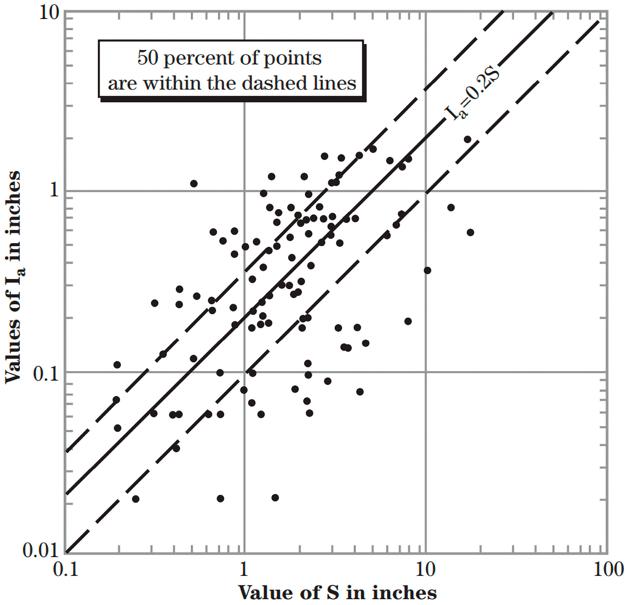
4.1. Validity of Ia = 0.2S and the Newly Proposed Correlation of Ia = SL

Previous research has shown that the linear correlation (Ia = 0.2S) proposed by the SCS in 1954 to simplify its rainfall runoff model, which is widely used as the conventional SCS runoff prediction (Equation (2)), lacks statistical verification even within its own datasets [23,34]. This has led to numerous reports of inaccuracies and inconsistencies in the model’s runoff predictions by studies worldwide [17,18,24,34,38,49,51,52,53,54,55].
The SCS proposed a linear correlation of Ia = 0.2S in 1954 to simplify Equation (1) [13,14,15], but two studies have shown it to be statistically insignificant even to the original SCS dataset. These studies found that the best correlation should be Ia = 0.111S or Ia = 0.112S, instead of Ia = 0.2S [34,35]. Unlike previous studies, which calibrated the SCS-CN runoff predictive model based on Ia = λS, this study assessed the use of a non-linear correlation between Ia and S in the form of Ia = SL to simplify Equation (1) and revise the SCS-CN rainfall runoff model to improve its runoff estimates.
The use of Equation (2) in education raises serious concerns. It could lead students to adopt a simplified and flawed approach for runoff prediction, which would have a wide impact on related fields such as water resource management, environmental science, and civil engineering. As Equation (2) was found to be statistically insignificant even to its original dataset, this can mislead students into following a faulty rainfall runoff model. Additionally, continued use of Equation (2) in educational resources such as textbooks, software, government agency handbooks, and training perpetuates the use of an unreliable runoff prediction method. Updating and enhancing the SCS-CN model for educational purposes is crucial to ensure that students and professionals have accurate and effective tools for runoff prediction. Only with the corrected rainfall runoff model can the reliability and accuracy of the model, along with the related software, be improved and applied in industry in the future.

4.2. Application of Newly Calibrated Runoff Predictive Models

This study uses the largest collected rainfall runoff dataset from watersheds in Malaysia under the DID-HP 11 and DID-HP 27 programs for analysis. The results showed that the power regression model was better at predicting runoff compared to the conventional SCS-CN rainfall runoff (Equation (2)), where the accuracy and the consistency of the model had been improved significantly. The comparison of the model performance is summarized in Appendix D. The ratios of Ia to S were found to be mostly 5% or lower and far from the SCS’s proposed value of 0.2 (20%) [17,18,24,34,38,49,51,52,53,54,55]. This shows that the calibrated and revised models are able to produce outcomes that are in line with the published results from past research. In addition, the newly revised model has been tested with multiple datasets across different catchments in Malaysia, China, and Greece and has demonstrated enhanced runoff estimation accuracy to formulate the CN runoff model with the power correlation of Ia = SL [12].
This study also highlights the importance of designing flood control infrastructure based on the maximum estimated runoff amount. The runoff estimates based on the upper limit of the BCa 99% CI for CN0.2 were significantly higher than the estimates based on the optimum CN0.2 values. Not designing flood prevention infrastructure based on the maximum estimate could result in an underestimation of the runoff volume of approximately 20 Olympic-sized swimming pools per 1 km2 area (Table 6). This revised CN model has the potential to improve water resource management by providing more accurate runoff predictions for different soil and hydrological conditions. This can aid in making better informed decisions about water availability and flood hazards, as accurate quantification of runoff is crucial for managing water resources, particularly for predicting floods.
The revised CN model allows for a more precise calculation of runoff from a specific region considering various soil and hydrological conditions. This information is critical for effective water resource management, as it predicts water availability and helps assess flood risks, reducing harm to infrastructure, lives, and finances caused by floods. It is crucial for professionals in the field to be familiar with the improved SCS rainfall runoff model and consider using it in their work. This revised model has the ability to give more accurate and reliable predictions of runoff, which can greatly enhance water resource management and flood prediction outcomes. With the enhanced rainfall runoff model, potential flood issues can be coped with in a much more efficient way, helping practitioners reduce financial loss caused by flood damage and poor flood prevention planning.

4.3. Decadal Runoff Trend Analaysis in Both Peninsular Malaysia and East Malaysia

The increasing trend in runoff in both Peninsular Malaysia and East Malaysian watersheds over the decades is a matter of concern for flood mitigation. The amount of runoff, which is a measure of the flow of water, is an important factor in the prediction of flood hazards. By using the BCa 99% CI for CN0.2 calculation in both regions, it is possible to determine the maximum runoff across the decades, which indicates that the maximum runoff amount has increased over time. This trend highlights the need to be proactive in mitigating the risk of flooding. It is important for engineers and hydrologists in Malaysia to take note of this trend and plan flood control infrastructure accordingly. Proper planning and management of flood control infrastructure can help to mitigate the impact of floods and reduce the risk of damage to people, property, and the environment.
This study examined the link between deforestation and runoff. A correlation between decreasing forest area and increasing runoff amounts in Peninsular Malaysia and East Malaysia over the decades was established (Table 7, Table 8 and Table 9). This demonstrates that deforestation has contributed to the increase in runoff. These results align with previous research indicating that deforestation can lead to higher runoff. Therefore, it is crucial for federal agencies to implement effective forest management strategies, such as afforestation or reforestation, to mitigate runoff and potential flood problems.
It is crucial to understand the impact of deforestation on runoff, as this can have significant implications for water resource management and flood mitigation. By implementing proper forest management strategies, the negative effects of deforestation can be mitigated, which can help to reduce the risk of flooding and improve water resource management. This highlights the importance of considering the relationship between deforestation and runoff in order to make informed decisions about the management of forested areas.

4.4. Exploring the Application of Machine Learning for Rainfall Runoff Prediction

In the last few decades, machine learning has become increasingly popular in hydrology research. Several machine learning techniques, including long short-term memory (LSTM), adaptive neuro-fuzzy inference systems (ANFIS), multilayer perceptron (MLP), wavelet neural networks (WNN), ensemble prediction systems (EPS), support vector machines (SVM), support vector regression (SVR), and artificial neural networks (ANN), have been introduced by researchers to enhance the precision and effectiveness of predictive models. Hybrid machine learning approaches, such as ANFIS and WNN, have also been found to offer improved accuracy and performance for long-term and short-term rainfall runoff models [44]. Furthermore, machine learning can be applied to resolve the issue of a lack of time series data for flow hydrographs due to the absence of gauged stations by using flood modelling methods, such as the reverse flood routing model, HEC-RAS, and GIS flood maps. The new rainfall runoff model proposed in this study may also benefit from being combined with machine learning techniques [19,20,21].

5. Conclusions

This study employed a new correlation (Ia = SL) to calibrate the SCS rainfall runoff prediction framework (Equation (1)) using inferential statistics. It assessed the accuracy of the newly calibrated model, analyzed the decadal runoff trends in Malaysia, and studied the effect of deforestation on the runoff trends. The main findings are:
  • This study demonstrated the unreliability of the SCS’s proposed relation of Ia = 0.2S, indicating a need to update the SCS runoff prediction model. The new power correlation of Ia = SL shows improved accuracy in runoff prediction. The results align with previous global studies, indicating an Ia to S ratio of around 5% or less, which is significantly different from the traditional value of 0.2 (20%) proposed by the SCS. On average, the power regression model exhibits a 138% higher predictive accuracy than the conventional SCS-CN model, as measured by the KGE index.
  • This study emphasizes designing flood control infrastructure based on the maximum estimated runoff amount. Not using this estimate could result in a 50,100 m3 underestimation of the runoff volume per 1 km2 watershed area in Malaysia, as indicated by the difference between the optimum CN0.2 values and the upper limit of the BCa 99% CI for CN0.2.
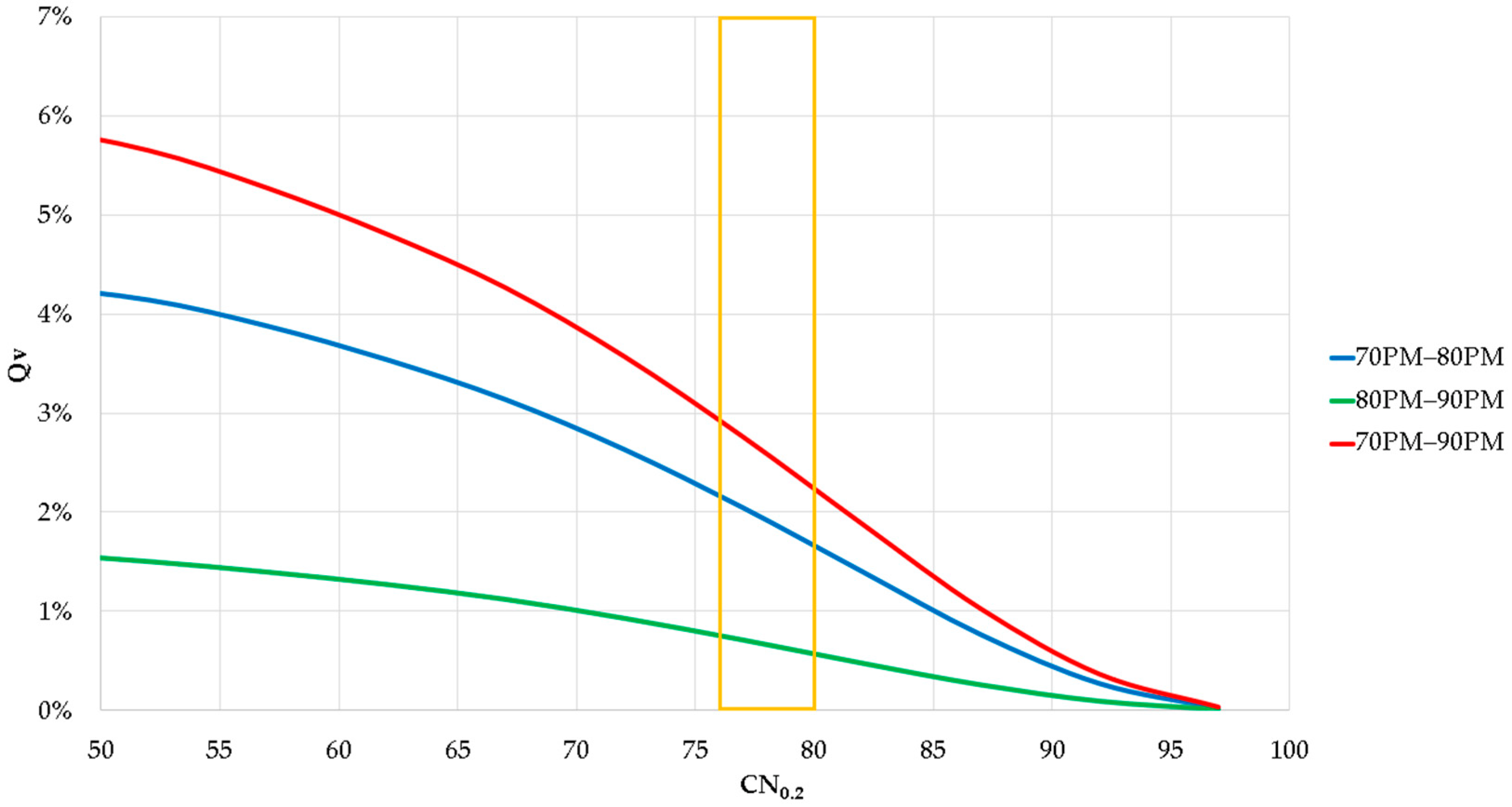
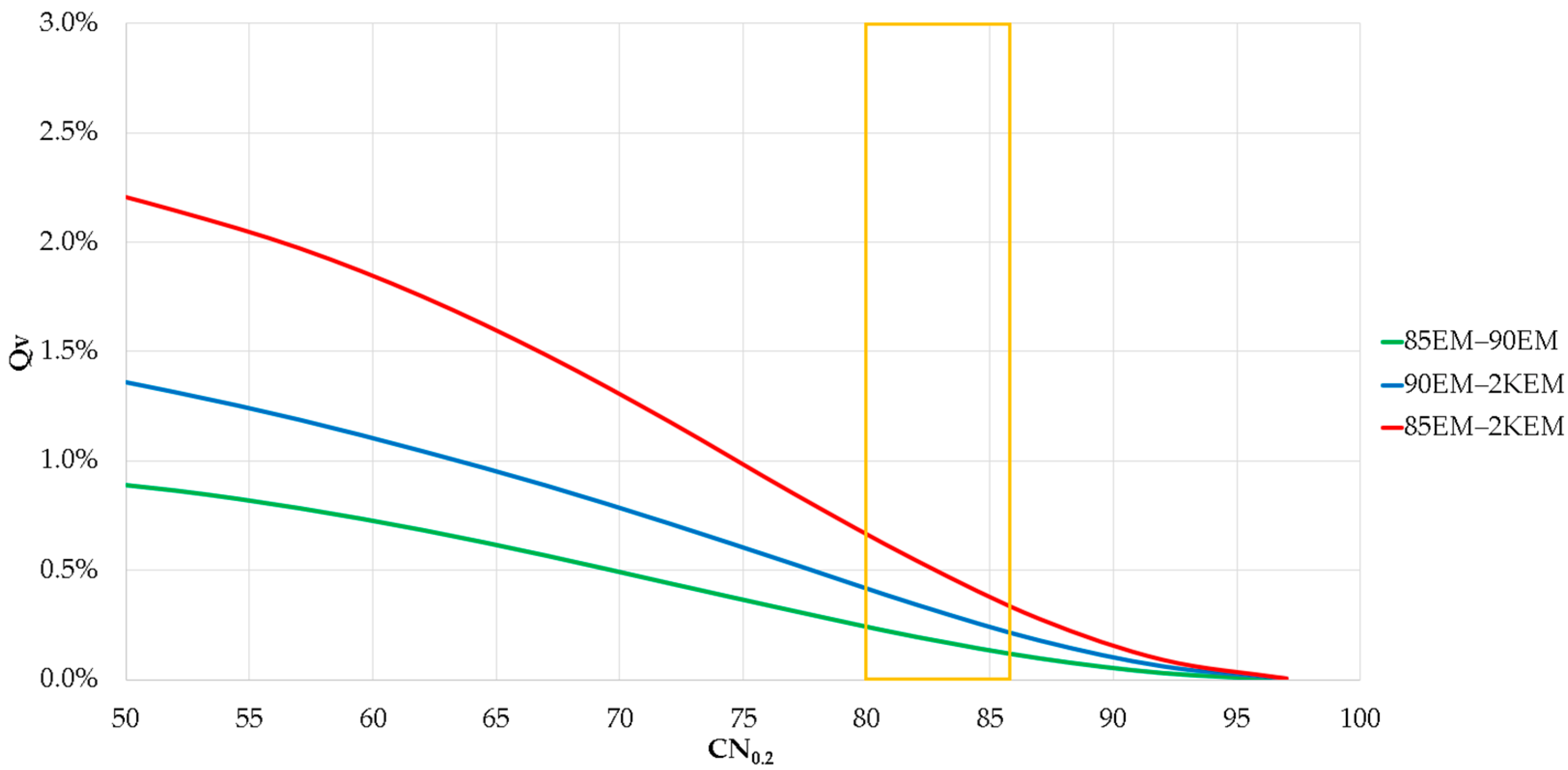
  • This study found a strong correlation between decreasing forest area and increasing runoff difference in Malaysia over time. Peninsular Malaysia saw a 25% reduction in forest area from the 1970s to the 1990s, and East Malaysia experienced a 9% reduction from the 1980s to the 2010s. This was accompanied by an increase in decadal runoff difference, with the most significant increases of 108% in Peninsular Malaysia from the 1970s to the 1990s and 32% in East Malaysia from the 1980s to the 2010s.
  • The proposed methodology requires a minimum dataset of 25 data pairs for accurate inferential results and relies on the bootstrap BCa method for optimizing key variables and formulating a new runoff predictive model. Therefore, using statistical software with this method is essential. Future studies may consider incorporating machine learning methods to further enhance the model’s performance.

Author Contributions

Conceptualization, L.L.; methodology, L.L.; software, J.F.K. and L.L.; validation, J.F.K. and L.L.; formal analysis, J.F.K. and L.L.; investigation, J.F.K. and L.L.; resources, L.L.; data curation, L.L.; writing—original draft preparation, J.F.K. and L.L.; writing—review and editing, J.F.K., S.L. and L.L.; visualization, J.F.K., S.L. and L.L.; supervision, L.L.; project administration, L.L.; funding acquisition, L.L. All authors have read and agreed to the published version of the manuscript.

Funding

The research was supported by Ministry of Higher Education (MoHE) through the Fundamental Research Grant Scheme (FRGS/1/2021/WAB07/UTAR/02/1) and was partly supported by the Brunsfield Engineering Sdn. Bhd., Malaysia (Brunsfield 8013/0002 & 8126/0001).

Data Availability Statement

The data that support the findings of this study are available from the corresponding author, Ling Lloyd, at linglloyd@utar.edu.my upon reasonable request.

Conflicts of Interest

The authors declare no conflict of interest.

Appendix A

Past studies rearranged Equation (1) into a general formula for S to obtain the corresponding S values according to P and Q datasets. However, the SCS proposed that Ia = 0.2S and simplified Equation (1) to Equation (2), whereby P must be > 0.2S for runoff (Q) to occur.
In this study, the power regression model was incorporated into the SCS-CN rainfall runoff model with the aim of obtaining a simplified closed-form general formula for S in the newly calibrated runoff model. The newly proposed power correlation between Ia and S in the form of Ia = SL was substituted into Equation (1):
Q = P S L 2 P S L + S Q P S L + S = ( P   S L ) 2 QP QS L + SQ = P 2 2 PS L + S 2 L
QP P 2 =   S 2 L + Q 2 P S L + Q 2 P 2 2 SQ Q 2 P 2 2
( S L + Q 2 P 2 ) 2 = 1 4 4 SQ + 4 PQ + Q 2 4 PQ + 4 P 2 4 P 2 ( 2 S L + Q 2 P ) 2 = 4 SQ + Q 2
The general formula for S in its simplest form is presented in Equation (A1), as no further simplification is possible. Currently, there is no closed form for the general formula for S from the revised model, so a numerical analysis technique will be used to determine the S value using the general formula for S, also referred to as Equation (6) in the article.

Appendix B. Refer to Section 2.4, Equation (6) in [47] and Section 2, Equation (8) in [56]

We managed to rearrange Equation (1) into a general formula for S in our past studies (when Ia = λS) as below [47,56]:
S λ = P λ 1 Q 2 λ PQ P 2 + P λ 1 Q 2 λ 2 λ
If λ = 0.2, Equation (A2) can be simplified to become Equation (7).
Equation (7) represents the general equation for S when λ = 0.2, allowing for calculation of S0.2 from P and Q values. Equation (7) is identical to Hawkins’ previous study [35,49]. By using Equation (7), S0.2 can be calculated for each P–Q pair from all study sites and the correlation between S0.2 and Sλ can be established using SPSS. The correlation equation can then be integrated into the SCS-CN curve number model to determine CN0.2 for each dataset.

Appendix C

In this study, the SCS model calibration steps and CN0.2 value derivation are summarized as below:
  • The SCS stated that Ia = λS, while the effective rainfall (Pe) = P − Ia, and therefore Equation (1) ( Q = P I a P I a + S ) can be expressed as:
Q = P e 2 P e + S   or   S = P e 2 Q   P e
This study follows the same framework, except that Ia = SL instead of Ia = λS
2.
Given a P–Q dataset, the corresponding Li and Si values to Pi and Qi can be calculated through numerical analysis technique with Equation (6) or (A1). To date, there is no closed form for the general equation for S. Therefore, a numerical analysis technique will be used to solve for the corresponding Si values.
3.
With bootstrap, a BCa procedure (selects 95–99% confidence interval level) to generate the confidence interval (CI) for derived Li and Si datasets and check for its dataset normality in SPSS (or other statistical software):
(a)
If the dataset is normally distributed, the optimum S and L values are found from the mean BCa CI to formulate a new runoff predictive model.
(b)
Otherwise, the S and L optimization process will refer to the median BCa CI (denote the optimum value of both parameters as Loptimum and Soptimum).
4.
To formulate the new SCS-CN rainfall runoff model, both Loptimum and Soptimum values are substituted into Equation (1) with Ia = SL.
5.
The corresponding Si values with the same P–Q dataset are computed, along with the Loptimum value with Equations (A1) or (6) through numerical analysis technique.
6.
Given (Pi, Qi) data pairs and λ = 0.2, S0.2i values are computed with Equations (A3) or (7).
7.
S0.2i (from step 6) and Si (from step 5) values are correlated to obtain a correlation equation between S0.2i and Si via SPSS for curve number (CN0.2) value derivation.
8.
The S correlation equation from step 7 is substituted into the SCS curve number formula ( CN 0.2 = 25,400 S 0.2 + 254 ) to derive the CN0.2 value.
Note: Refer to the example discussion from Section 2.3 in the article.

Appendix D

The performance of the decadal model was evaluated in Section 3.1 and shown in Table 1 and Table 2. To compare the runoff predictive ability of the newly calibrated model and Equation (2), the performance of the latter had to be determined first. In Equation (2), the value of λ was set to 0.2, as suggested by the SCS, and the optimum S value was determined with the constraint of S being greater than 0.
The optimum S value for the conventional model was determined and then the Nash–Sutcliffe index, the bias, and the KGE index were also calculated. A comparison of the performance between the recalibrated model and the conventional model was then made using the Nash–Sutcliffe index (E), the bias, and the Kling–Gupta efficiency index (KGE) for each decadal model in Peninsular Malaysia and East Malaysia, as shown in Table A1.
The results in Table A1 show that, for all the decadal models, the KGE index of the power regressed model is higher than that of the conventional SCS-CN model. Since the KGE index considers both the bias and the flow variability error, it provides a more accurate and meaningful evaluation compared to the Nash–Sutcliffe index (E), which is not sensitive to bias. The overall results indicate that the power regressed model improves the accuracy and consistency of the rainfall runoff model, as demonstrated by its higher E index, reduced bias, and higher KGE index.
Table A1. Comparison of the performance of the recalibrated model with the conventional model, based on the Nash–Sutcliffe index (E), the bias, and the Kling–Gupta efficiency index (KGE) for each decadal model in Peninsular Malaysia and East Malaysia, with the constraint Ia < P applied to the conventional SCS-CN model.
Decadal ModelPower Regressed ModelConventional SCS-CN Model
EBiasKGEEBiasKGE
70PM0.94100.9680.87612.290.579
80PM0.9060.4970.9470.50624.850.346
90PM0.89200.9250.80110.750.733
85EM −0.387−1.9100.307−0.1089.49−0.401
90EM 0.78800.7130.31612.220.195
2KEM0.73000.8660.30212.720.391
Notes: A positive Bias in Equation (2) indicates that the conventional SCS-CN model overestimated the runoff depths for all datasets in this study. On average, the power regression model shows a 138% improvement in predictive accuracy compared to the conventional SCS-CN model, as measured by the KGE index.
The 95% and 99% BCa confidence intervals of λ for each decadal model in Peninsular Malaysia and East Malaysia were determined with the SPSS according to the methodology of one of our past studies [38] and tabulated in Table A2.
Table A2. The BCa confidence intervals of λ for each decadal model in Peninsular Malaysia and East Malaysia for the conventional SCS-CN model.
Decadal ModelStd. Dev.95% BCa CI for λ99% BCa CI for λ
LowerUpperVariation LowerUpperVariation
70PM0.1230.0570.08244.04%0.0530.08966.32%
80PM0.0880.0140.01827.48%0.0140.02040.91%
90PM0.1320.0320.04646.07%0.0320.05469.27%
85EM 0.2590.0280.072158.77%0.0250.080218.59%
90EM 0.0780.0060.00942.03%0.0060.00966.27%
2KEM0.1760.0140.053274.04%0.0140.061349.23%
The variability of the BCa confidence interval and the non-zero standard deviation values showed that the λ value is not a constant, as proposed by the SCS, but a variable. The proposed value of λ by SCS (λ = 0.2) does not fall within any 95% and 99% confidence intervals in this study (Table A2). This indicates that the conventional SCS-CN model, Equation (2), is not even statistically valid at the alpha = 0.05 level and therefore cannot be adopted for runoff estimates for any dataset in this study.

Appendix E

As an example, this section shows the procedure to formulate the runoff prediction model for East Malaysia’s 2KEM dataset model.
The runoff equation for the 2KEM dataset model is as follows, when the optimum L = 0.316:
Q 0.316 = P S 0.316 0.316 2 P S 0.316 0.316 + S 0.316
The best S correlation equation for the 2KEM dataset model was identified in SPSS as follows:
S0.2 = S0.3160.896
where the equation can be rearranged as:
S0.316 = S0.21.115
By substituting the S correlation back into the runoff equation, the runoff equation is shown as below:
Q 0.316 = P ( S 0.2 1.115   ) 0.316 2 P ( S 0.2 1.115   ) 0.316 + ( S 0.2 1.115   )
The above runoff equation can be re-expressed using the CN0.2 as shown below. Equation (10) will be utilized to express S0.2 in terms of CN0.2, and the resulting runoff model in terms of P and CN0.2 will be expressed as follows. After further simplification of the equation, the simplified recalibrated runoff equation in terms of P and CN0.2 for the 2KEM dataset model is presented as follows:
Q 0.316 = P 254 100 CN 0.2 1 1.115 0.316 2 P 254 100 CN 0.2 1 1.115 0.316 + 254 100 CN 0.2 1 1.115
Q 0.316 = P 7.032 100 CN 0.2 1 0.352   2 P 7.032 100 CN 0.2 1 0.352 + 480.164 100 CN 0.2 1 1.115
With a similar derivation approach, decadal models in this study can be derived as shown in Table A3:
Table A3. Equations for each decadal model in Peninsular Malaysia and East Malaysia.
Peninsular Malaysia
Decadal DatasetsDecadal Model Equations
1970s
(70PM)
Q 0.168 = P 2.947 100 CN 0.2 1 0.195   2 P 2.947 100 CN 0.2 1 0.195 + 619.458 100 CN 0.2 1 1.161
1980s
(80PM)
Q 0.228 = P 4.186 100 CN 0.2 1 0.259   2 P 4.186 100 CN 0.2 1 0.259 + 530.489 100 CN 0.2 1 1.133  
1990s
(90PM)
Q 0.232 = P 4.237 100 CN 0.2 1 0.261   2 P 4.237 100 CN 0.2 1 0.261 + 501.913 100 CN 0.2 1 1.123  
East Malaysia
1985s
(85EM)
Q 0.332 = P 7.959 100 CN 0.2 1 0.375   2 P 7.959 100 CN 0.2 1 0.375 + 518.869 100 CN 0.2 1 1.129  
1990s
(90EM)
Q 0.274 = P 5.505 100 CN 0.2 1 0.308   2 P 5.505 100 CN 0.2 1 0.308 + 507.502 100 CN 0.2 1 1.125
2000s
(2KEM)
Q 0.316 = P 7.032 100 CN 0.2 1 0.352   2 P 7.032 100 CN 0.2 1 0.352 + 480.164 100 CN 0.2 1 1.115  

Appendix F

According to Table 6 in Section 3.1, the optimum value of CN0.2 in the 2KEM dataset in East Malaysia is 73.76. With the highest recorded rainfall depth of 224 mm in the same decade, the estimated runoff can be calculated using Equation (10) for the S correlation and Equation (12) as 129.48 mm. As per Appendix E, the runoff equation for the 2KEM dataset model in terms of P and CN0.2 has been recalibrated and is presented as follows:
Q 0.316 = P 254 100 CN 0.2 1 1.115 0.316 2 P 254 100 CN 0.2 1 1.115 0.316 + 254 100 CN 0.2 1 1.115    
As the optimum (collective representation of) CN0.2 = 73.76 and with a rainfall depth of 224 mm, the estimated runoff obtained is as follows:
Q 0.316 = 224 254 100 73.76 1 1.115 0.316 2 224 254 100 73.76 1 1.115 0.316 + 254 100 73.76 1 1.115 Q 0.316 = 224 90.36 1.115 0.316 2 224 90.36 1.115 0.316 + 90.36 1.115 Q 0.316 = 224 4.89 2 224 4.89 + 151.68 Q 0.316 = 219.11 2 370.79 Q 0.316 = 129.48   mm
A higher CN0.2 value will result in a higher runoff amount; thus, to obtain the maximum runoff amount, the 99% BCa upper limit and the CN0.2 will be selected to estimate the maximum runoff amount. As shown in Section 3.1 (Table 5), the 99% BCa lower and upper limit of CN0.2 for the 2KEM model were 72.15 and 88.32 respectively.
Since the corresponding 99% BCa upper limit of the CN0.2 = 88.32, the estimated runoff amount can also be obtained with a similar approach as shown above, resulting in a value of 179.58 mm. Comparing both the runoff amount estimated based on the collective representation (optimum CN0.2) and the 99% BCa upper limit of CN0.2, a runoff difference (Qv) of 50.10 mm is observed.
If Qv = 179.58–129.48 mm = 50.10 mm, thus
Q v = 50.10   1000   m
Q v = 0.05010   m  
For the calculation of the runoff volume, for illustration purposes, the watershed is set to be an area of 1 km2. Then, the calculation of the volume in the watershed can be shown as follows:
1   km = 1000   m 1   km 2 = 1000 2   m 2 Runoff   Volume   Difference = Watershed   Area   × Runoff   Depth   Difference Runoff   Volume   Difference = 1   km 2 × Q v Runoff   Volume   Difference = 1000 2   m 2 × 0.05010   m Runoff   Volume   Difference = 50,100   m 3 / 1   km 2   watershed   area
Therefore, for a one square kilometer watershed, the difference in runoff volume between the maximum runoff estimate and the estimated runoff based on the optimum CN0.2 is 50,100 cubic meters, or 50.1 million liters. This shows that practitioners should consider not only the runoff estimate based on the optimum CN0.2 value, but also the maximum estimated runoff, when designing flood control infrastructure, in order to reduce the risk of overflow due to inadequate capacity of flood control structures such as dams and flood walls.

Appendix G

To emphasize the significance of calibrating the rainfall runoff model using a new correlation model as proposed in this study, Figure A1 and Figure A2 were created to demonstrate the impact of not implementing an appropriate correlation model in Peninsular Malaysia and East Malaysia. The decadal model which recorded the maximum rainfall was selected for both Peninsular Malaysia (70PM) and East Malaysia (90EM) to highlight the differences in runoff between the CN0.2 values.
In Section 3.1, Table 1 and Table 2 show that the L values for 70PM and 90EM were 0.168 and 0.274, respectively. The initial abstraction value (Ia) for both 70PM and 90EM can be determined by the following equations:
70 PM :   I a = S 0.168
90 EM :   I a = S 0.274
From Table A3 in Appendix E, the calibrated runoff model was derived in terms of CN0.2 as follows for 70PM and 90EM (the derivation of the calibrated runoff model is summarized in Appendix E).
70 PM :   Q 0.168 = P 2.947 100 CN 0.2 1 0.195   2 P 2.947 100 CN 0.2 1 0.195 + 619.458 100 CN 0.2 1 1.161
90 EM :   Q 0.274 = P 5.505 100 CN 0.2 1 0.308   2 P 5.505 100 CN 0.2 1 0.308 + 507.502 100 CN 0.2 1 1.125
Meanwhile, the conventional SCS-CN rainfall runoff model can be derived in terms of CN0.2 as follows:
Q 0.2 = P 0.2 S 2 P 0.2 S + S Q 0.2 = P 0.2 S 2 P + 0.8 S
With Equation (10), the conventional SCS-CN rainfall runoff will be expressed in terms of CN0.2 (Equation (A7)) as follows:
Q 0.2 = P 0.2 254 × 100 CN 0.2 1 2 P + 0.8 254 × 100 CN 0.2 1
Q 0.2 = P 50.8 100 CN 0.2 1 2 P + 203.2 100 CN 0.2 1
Once the calibrated runoff models for both decadal models and the conventional SCS-CN model were identified, the models were used to determine the runoff difference (Qv) between the runoff obtained from the conventional rainfall runoff model and the one obtained from the calibrated model under the conditions of maximum rainfall amount. For Peninsular Malaysia, the maximum rainfall amount (P) was nearly 490 mm, while for East Malaysia, the maximum rainfall amount (P) was approximately 580 mm.
The runoff difference (Qv) was calculated by Equations (A8) and (A9) as follows:
70 PM :   Q v = Q 0.2   A 7 Q 0.168   A 5
90 EM :   Q v = Q 0.2   A 7 Q 0.274   A 6
The Qv obtained from Equation (A8) and Equation (A9) were plotted against different CN0.2 values, respectively. Figure A1 and Figure A2 show the runoff differences between the conventional SCS-CN rainfall runoff model (Equation (2)) and the calibrated model across different CN0.2 values in both Peninsular Malaysia in the 1970s and East Malaysia in the 1990s.
From the observations in Figure A1 and Figure A2, the highest runoff difference (Qv) in Peninsular Malaysia was nearly 65 mm at a maximum rainfall amount (P) of 490 mm, while in East Malaysia, the highest runoff difference (Qv) was nearly 45 mm at a maximum rainfall amount (P) of 580 mm. This indicates a significant overprediction of the runoff depth if the calibrated model is not used.
Figure A1. The runoff difference between the conventional SCS-CN rainfall runoff model and the calibrated model across different CN0.2 values in Peninsular Malaysia during the 1970s. Note: 490 mm is the highest recorded rainfall amount in Peninsular Malaysia.
Water 15 01392 g0a1
Figure A2. The runoff difference between the conventional SCS-CN rainfall runoff model (Equation (2)) and the calibrated model across different CN0.2 values in East Malaysia during the 1990s. Note: 580 mm is the highest recorded rainfall amount in East Malaysia.
Water 15 01392 g0a2
As mentioned in Appendix E, a difference of 1 mm in runoff can result in a runoff volume difference of 1000 m3/1 km2 in the watershed area in Malaysia. This highlights the crucial need to revise and calibrate the rainfall runoff model using the power regression model of Ia = SL. As illustrated in Figure A1 and Figure A2, without proper model calibration, a volume difference of nearly 65,000 m3 or 45,000 m3 in runoff could be overestimated in both Peninsular Malaysia and East Malaysia. This may lead to potential opportunity loss for flood prevention planning based on an overprediction of the conventional SCS-CN rainfall runoff model (Equation (2)).

References

  1. Yang, T.H.; Liu, W.C. A General Overview of the Risk-Reduction Strategies for Floods and Droughts. Sustainability 2020, 12, 2687. [Google Scholar] [CrossRef] [Green Version]
  2. Zhang, W.; Luo, M.; Gao, S.; Chen, W.; Hari, V.; Khouakhi, A. Compound Hydrometeorological Extremes: Drivers, Mechanisms and Methods. Front. Earth Sci. 2021, 9, 673495. [Google Scholar] [CrossRef]
  3. Garner, G.; van Loon, A.F.; Prudhomme, C.; Hannah, D.M. Hydroclimatology of Extreme River Flows. Freshw. Biol. 2015, 60, 2461–2476. [Google Scholar] [CrossRef]
  4. Morin, E.; Harats, N.; Jacoby, Y.; Arbel, S.; Getker, M.; Arazi, A.; Grodek, T.; Ziv, B.; Dayan, U. Studying the Extremes: Hydrometeorological Investigation of a Flood-Causing Rainstorm Over Israel. Adv. Geosci. 2007, 12, 107–114. [Google Scholar] [CrossRef] [Green Version]
  5. Nyeko-Ogiramoi, P.; Willems, P.; Ngirane-Katashaya, G. Trend and Variability in Observed Hydrometeorological Extremes in the Lake Victoria Basin. J. Hydrol. 2013, 489, 56–73. [Google Scholar] [CrossRef]
  6. Fattorelli, S.; Fontana, G.D.; Ros, D. Flood Hazard Assessment and Mitigation. In Floods and Landslides: Integrated Risk Assessment; Springer: Berlin/Heidelberg, Germany, 1999; pp. 19–38. [Google Scholar]
  7. Tsakiris, G. Flood Risk Assessment: Concepts, Modelling, Applications. Nat. Hazards Earth Syst. Sci. 2014, 14, 1361–1369. [Google Scholar] [CrossRef] [Green Version]
  8. Sitterson, J.; Knightes, C.; Parmar, R.; Wolfe, K.; Avant, B.; Muche, M. An Overview of Rainfall-Runoff Model Types. In Proceedings of the International Congress on Environmental Modelling and Software, Collins, CO, USA, 24–28 June 2018; p. 41. [Google Scholar]
  9. Nagure, A.S.; Shahapure, S.S. Effect of Watershed Characteristics on a Rainfall Runoff Analysis and Hydrological Model Selection-A Review. In Proceedings of the 2021 International Conference on Computing, Communication and Green Engineering (CCGE), Pune, India, 23–25 September 2021; IEEE: New York, NY, USA, 2021. [Google Scholar]
  10. Rezaie-Balf, M.; Zahmatkesh, Z.; Kim, S. Soft Computing Techniques for Rainfall-Runoff Simulation: Local Non–Parametric Paradigm vs. Model Classification Methods. Water Resour. Manag. 2017, 31, 3843–3865. [Google Scholar] [CrossRef]
  11. Vafakhah, M.; Janizadeh, S.; Bozchaloei, S.K. Application of Several Data-Driven Techniques for Rainfall-Runoff Modeling. Ecopersia 2014, 2, 455–469. [Google Scholar]
  12. Lee, K.K.F.; Ling, L.; Yusop, Z. The Revised Curve Number Rainfall-Runoff Methodology for an Improved Runoff Prediction. Water 2023, 15, 491. [Google Scholar] [CrossRef]
  13. N.E.D.C. Engineering Hydrology Training Series. In Module 205-SCS Runoff Equation; N.E.D.C.: London, UK, 1997; Available online: https://d32ogoqmya1dw8.cloudfront.net/files/geoinformatics/steps/nrcs_module_runoff_estimation.pdf (accessed on 8 July 2022).
  14. Soil Conservation Service (S.C.S.). National Engineering Handbook; Section 4; US Soil Conservation Service: Washington, DC, USA, 1964; Chapter 10. Available online: https://directives.sc.egov.usda.gov/RollupViewer.aspx?hid=17092 (accessed on 10 July 2022).
  15. USDA; NRCS. National Engineering Handbook, Part 630 Hydrology; US Soil Conservation Service: Washington, DC, USA, 1964; Chapter 10. [Google Scholar]
  16. Mishra, S.K.; Suresh Babu, P.; Singh, V.P. SCS-CN Method Revisited. In Advances in Hydraulics and Hydrology; Water Resources Publications: Littleton, CO, USA, 2007. [Google Scholar]
  17. Tan, W.J.; Ling, L.; Yusop, Z.; Huang, Y.F. New Derivation Method of Region Specific Curve Number for Urban Runoff Prediction at Melana Watershed in Johor, Malaysia. IOP Conf. Ser. Mater. Sci. Eng. 2018, 401, 012008. [Google Scholar] [CrossRef]
  18. Yuan, L.; Sinshaw, T.; Forshay, K.J. Review of Watershed-Scale Water Quality and Nonpoint Source Pollution Models. Geosciences 2020, 10, 25. [Google Scholar] [CrossRef] [PubMed] [Green Version]
  19. Mosavi, A.; Ozturk, P.; Chau, K. Flood Prediction Using Machine Learning Models: Literature Review. Water 2018, 10, 1536. [Google Scholar] [CrossRef] [Green Version]
  20. Fu, M.; Fan, T.; Ding, Z.; Salih, S.Q.; Al-Ansari, N.; Yaseen, Z.M. Deep Learning Data-Intelligence Model Based on Adjusted Forecasting Window Scale: Application in Daily Streamflow Simulation. IEEE Access 2020, 8, 32632–32651. [Google Scholar] [CrossRef]
  21. Kaya, C.M.; Tayfur, G.; Gungor, O. Predicting Flood Plain Inundation for Natural Channels Having No Upstream Gauged Stations. J. Water Clim. Chang. 2019, 10, 360–372. [Google Scholar] [CrossRef] [Green Version]
  22. Hawkins, R.H.; Moglen, G.E.; Ward, T.J.; Woodward, D.E. Updating the Curve Number: Task Group Report. In Proceedings of the Watershed Management 2020, Henderson, NV, USA, 20–21 May 2020; American Society of Civil Engineers: Reston, VA, USA, 2020; pp. 131–140. [Google Scholar]
  23. Hawkins, R.H.; Yu, B.; Mishra, S.K.; Singh, V.P. Another Look at SCS-CN Method. J. Hydrol. Eng. 2001, 6, 451–452. [Google Scholar] [CrossRef]
  24. Hawkins, R.; Ward, T.J.; Woodward, E.; van Mullem, J.A. Continuing Evolution of Rainfall-Runoff and the Curve Number Precedent. In Proceedings of the 2nd Joint Federal Interagency Conference, Las Vegas, NV, USA; 2010; pp. 1–12. [Google Scholar]
  25. Qin, T. Urban Flooding Mitigation Techniques: A Systematic Review and Future Studies. Water 2020, 12, 3579. [Google Scholar] [CrossRef]
  26. Cooper, R.J.; Hiscock, K.M.; Lovett, A.A. Mitigation Measures for Water Pollution and Flooding. In Landscape Planning with Ecosystem Services; von Haaren, C., Lovett, A., Albert, C., Eds.; Landscape series; Volume 24, Springer: Dordrecht, The Netherlands, 2019. [Google Scholar] [CrossRef]
  27. Xie, J.; Chen, H.; Liao, Z.; Gu, X.; Zhu, D.; Zhang, J. An Intergrated Assessment of Urban Flooding Mitigation Strategies for Robust Decision Making. Environ. Model. Softw. 2017, 95, 143–155. [Google Scholar] [CrossRef]
  28. Danáčová, M.; Földes, G.; Labat, M.M.; Kohnová, S.; Hlavčová, K. Estimating the Effect of Deforestation on Runoff in Small Mountainous Basins in Slovakia. Water 2020, 12, 3113. [Google Scholar] [CrossRef]
  29. Li, Y.; Liu, C.; Zhang, D.; Liang, K.; Li, X.; Dong, G. Reduced Runoff Due to Anthropogenic Intervention in the Loess Plateau, China. Water 2016, 8, 458. [Google Scholar] [CrossRef] [Green Version]
  30. Zhang, Y.; Xia, J.; Yu, J.; Randall, M.; Zhang, Y.; Zhao, T.; Pan, X.; Zhai, X.; Shao, Q. Simulation and Assessment of Urbanization Impacts on Runoff Metrics: Insights from Landuse Changes. J. Hydrol. 2018, 560, 247–258. [Google Scholar] [CrossRef]
  31. Zhai, R.; Tao, F. Contributions of Climate Change and Human Activities to Runoff Change in Seven Typical Catchments across China. Sci. Total Environ. 2017, 605–606, 219–229. [Google Scholar] [CrossRef]
  32. Li, C.; Liu, M.; Hu, Y.; Shi, T.; Qu, X.; Walter, M.T. Effects of Urbanization on Direct Runoff Characteristics in Urban Functional Zones. Sci. Total Environ. 2018, 643, 301–311. [Google Scholar] [CrossRef]
  33. Miyamoto, M.; Mohd Parid, M.; Noor Aini, Z.; Michinaka, T. Proximate and Underlying Causes of Forest Cover Change in Peninsular Malaysia. Policy Econ. 2014, 44, 18–25. [Google Scholar] [CrossRef] [Green Version]
  34. Tan, W.J.; Ling, L.; Yusop, Z.; Huang, Y.F. Claim Assessment of a Rainfall Runoff Model with Bootstrap. In Proceedings of the Third International Conference on Computing, Mathematics and Statistics (iCMS2017); Springer: Singapore, 2019; pp. 287–293. [Google Scholar]
  35. Hawkins, R.H.; Khojeini, A.V. Initial Abstraction and Loss in the Curve Number Method. In Proceedings of the Arizona State Hydrological Society Proceedings, Las Vegas, NV, USA, 15 April 1980; Arizona-Nevada Academy of Science: Las Vegas, NV, USA, 1980; pp. 115–119. [Google Scholar]
  36. DID. Hydrological Procedure 27 Design Hydrograph Estimation for Rural Catchments in Malaysia; JPS, DID: Kuala Lumpur, Malaysia, 2010. Available online: https://www.water.gov.my/jps/resources/PDF/Hydrology%20Publication/Hydrological_Procedure_No_27_(HP_27).pdf (accessed on 24 February 2023).
  37. DID. Hydrological Procedure 11 Design Flood Hydrograph Estimation for Rural Catchments in Malaysia; JPS, DID: Kuala Lumpur, Malaysia, 2018. Available online: http://h2o.water.gov.my/man_hp1/HP11_2018.pdf (accessed on 24 February 2023).
  38. Ling, L.; Lai, S.H.; Yusop, Z.; Chin, R.J.; Ling, J.L. Formulation of Parsimonious Urban Flash Flood Predictive Model with Inferential Statistics. Mathematics 2022, 10, 175. [Google Scholar] [CrossRef]
  39. Efron, B.; Tibshirani, R.J. An Introduction to the Bootstrap; Chapman and Hall/CRC: Boca Raton, FL, USA, 1993; ISBN 978-0-412-04231-7. [Google Scholar]
  40. Davison, A.C. Cambridge Series In Statistical And Probabilistic; Cambridge University Press: New York, NY, USA, 1997; ISBN 978-0-511-67299-6. [Google Scholar]
  41. Efron, B. Large-Scale Inference: Empirical Bayes Methods for Estimation, Testing, and Prediction; Cambridge University Press: New York, NY, USA, 2010; ISBN 978-1-107-61967-8. [Google Scholar]
  42. Rochowicz, J.A.J. Bootstrapping Analysis, Inferential Statistics and EXCEL. Spreadsheets Edu. (Ejsie) 2010, 4, 1–23. [Google Scholar]
  43. Moriasi, D.N.; Arnold, J.G.; Van Liew, M.W.; Bingner, R.L.; Harmel, R.D.; Veith, T.L. Model Evaluation Guidelines for Systematic Quantification of Accuracy in Watershed Simulations. Trans. ASABE 2007, 50, 885–900. [Google Scholar] [CrossRef]
  44. Nash, J.E.; Sutcliffe, J.V. River Flow Forecasting through Conceptual Models Part I—A Discussion of Principles. J. Hydrol. 1970, 10, 282–290. [Google Scholar] [CrossRef]
  45. Knoben, W.J.M.; Freer, J.E.; Woods, R.A. Technical Note: Inherent Benchmark or Not? Comparing Nash–Sutcliffe and Kling–Gupta Efficiency Scores. Hydrol. Earth Syst. Sci. 2019, 23, 4323–4331. [Google Scholar] [CrossRef] [Green Version]
  46. Gupta, H.V.; Kling, H.; Yilmaz, K.K.; Martinez, G.F. Decomposition of the Mean Squared Error and NSE Performance Criteria: Implications for Improving Hydrological Modelling. J. Hydrol. 2009, 377, 80–91. [Google Scholar] [CrossRef] [Green Version]
  47. Ling, L.; Yusop, Z.; Ling, J.L. Statistical and Type II Error Assessment of a Runoff Predictive Model in Peninsula Malaysia. Mathematics 2021, 9, 812. [Google Scholar] [CrossRef]
  48. Hawkins, R.H.; Ward, T.J.; Woodward, D.E.; van Mullem, J.A. Curve Number Hydrology: State of the Practice; American Society of Civil Engineers: Reston, VA, USA, 2009. [Google Scholar]
  49. Tedela, N.H.; McCutcheon, S.C.; Rasmussen, T.C.; Hawkins, R.H.; Swank, W.T.; Campbell, J.L.; Adams, M.B.; Jackson, C.R.; Tollner, E.W. Runoff Curve Numbers for 10 Small Forested Watersheds in the Mountains of the Eastern United States. J. Hydrol. Eng. 2012, 17, 1188–1198. [Google Scholar] [CrossRef] [Green Version]
  50. Miles, J. R Squared, Adjusted R Squared. In Wiley StatsRef: Statistics Reference Online; Wiley: Hoboken, NJ, USA, 2014. [Google Scholar]
  51. Hawkins, R.H.; Theurer, F.D.; Rezaeianzadeh, M. Understanding the Basis of the Curve Number Method for Watershed Models and TMDLs. J. Hydrol. Eng. 2019, 24, 06019003. [Google Scholar] [CrossRef]
  52. Baltas, E.A.; Dervos, N.A.; Mimikou, M.A. Technical Note: Determination of the SCS Initial Abstraction Ratio in an Experimental Watershed in Greece. Hydrol. Earth Syst. Sci. 2007, 11, 1825–1829. [Google Scholar] [CrossRef] [Green Version]
  53. Mishra, S.K.; Singh, V.P. Another Look at SCS-CN Method. J. Hydrol. Eng. 1999, 4, 257–264. [Google Scholar] [CrossRef]
  54. Yu, B. Discussion of “Another Look at SCS-CN Method” by Bofu Yu. J. Hydrol. Eng. 2001, 6, 451. [Google Scholar] [CrossRef]
  55. Jackson, T.J.; Rawls, W.J. SCS URBAN CURVE NUMBERS FROM A LANDSAT DATA BASE. J. Am. Water Resour. Assoc. 1981, 17, 857–862. [Google Scholar] [CrossRef]
  56. Ling, L.; Yusop, Z.; Yap, W.S.; Tan, W.L.; Chow, M.F.; Ling, J.L. A Calibrated, Watershed-Specific SCS-CN Method: Application to Wangjiaqiao Watershed in the Three Gorges Area, China. Water 2020, 12, 60. [Google Scholar] [CrossRef] [Green Version]
Figure 1. The original SCS data points from NEH-4 [15].
Water 15 01392 g001
Figure 2. Location where the rainfall runoff datasets were collected for Peninsular Malaysia and East Malaysia [36,37].
Water 15 01392 g002
Figure 3. The decadal runoff trend for the interdecadal runoff difference between 70PM and 80PM, 80PM and 90PM, and 70PM and 90PM. The yellow box highlights the 99% BCa confidence interval of CN0.2 for the Peninsular Malaysia dataset, in the range of 76–80.
Water 15 01392 g003
Figure 4. The decadal runoff trend for the interdecadal runoff difference between 85EM and 90EM, 90EM and 2KEM, and 85EM and 2KEM. The yellow box highlights the 99% BCa confidence interval of CN0.2 for the East Malaysia dataset, in the range of 80–86.
Water 15 01392 g004
Table 1. The optimum S (SL), L, Ia to S ratio, Nash–Sutcliffe index, bias, and KGE index for each decadal dataset in Peninsular Malaysia.
Decadal ModelLSL (mm)Ia/SEBIASKGE
70PM 0.168187.810.0130.94100.968
80PM 0.228183.310.0180.9060.4970.947
90PM0.232175.300.0190.89200.925
Table 2. The optimum S (SL), L, Ia to S ratio, Nash–Sutcliffe index, bias, and KGE index for each decadal dataset in East Malaysia.
Decadal ModelLSL (mm)Ia/SEBIASKGE
85EM 0.332152.230.035−0.387−1.9100.307
90EM 0.274121.110.0310.78800.713
2KEM0.316152.400.0320.73000.866
Table 3. The S correlation equation for each decadal group in Peninsular Malaysia.
Decadal ModelCorrelation EquationR2adjp-Value
70PMS0.2 = S0.1680.8510.987<0.001
80PMS0.2 = S0.2280.8810.998<0.001
90PMS0.2 = S0.2320.8890.998<0.001
Table 4. The S correlation equation for each decadal group in East Malaysia.
Decadal ModelCorrelation EquationR2adjp-Value
85EMS0.2 = S0.3320.8910.997<0.001
90EMS0.2 = S0.2740.8870.998<0.001
2KEMS0.2 = S0.3160.8960.998<0.001
Table 5. The optimum S, optimum CN0.2, and its corresponding BCa 99% CI for both Peninsular Malaysia and East Malaysia.
Peninsular Malaysia
Decadal Model BCa 99% CI for S (mm) BCa 99% CI for CN0.2
Optimum S (mm)LowerUpperOptimum CN0.2LowerUpper
70PM187.81137.59194.8574.6974.0979.36
80PM183.31137.60183.3172.0472.0476.83
90PM175.30120.37191.2171.9970.4178.22
East Malaysia
85EM152.2350.89152.2374.2674.2688.45
90EM121.1163.55127.2978.2977.5386.47
2KEM152.4050.49166.9573.7672.1588.32
Table 6. The highest recorded rainfall depth, the runoff estimation obtained from the optimum CN0.2, the maximum runoff amount estimated based on the BCa 99% CI of CN0.2, and the runoff difference between both estimated results through each decade for both Peninsular Malaysia and East Malaysia.
Peninsular Malaysia
Decadal Model
(Appendix E)
Highest Rainfall Depth Recorded (mm)Estimated Runoff Depth based on the Optimum CN0.2 (mm)Maximum Runoff Depth Estimated with Upper CN0.2 Limit (mm)Estimated Runoff Depth Difference (mm)
70PM485353.46380.5027.04
80PM420290.27314.1523.88
90PM306192.29217.3125.02
East Malaysia
85EM17588.13131.3343.20
90EM575472.20515.1642.96
2KEM224129.48179.5850.10
Table 7. The decadal changes in the amount and the corresponding percentage of forest area and runoff difference in Peninsular Malaysia.
Interdecadal PeriodForest Area Model Runoff Difference,
Qv, observed
(‘000 Ha)(%)(mm)(%)
1970s–1980s −1736.47−21.69%5.7142.26%
1980s–1990s−381.18−6.00%8.9146.36%
1970s–1990s−2032.94−25.39%14.62108.22%
Table 8. The decadal changes in the amount and the corresponding percentage of forest area and runoff difference in East Malaysia.
Interdecadal ModelForest Area Runoff Difference, Qv, observed
(‘000 Ha)%(mm)(%)
1987s–1990s−771−5.71%0.251.75%
1991s–2000s−1057−7.89%4.3529.90%
1987s–2010s−1167−9.24%4.6032.17%
Table 9. The best correlation models for each dataset and the corresponding adjusted R-squared.
Study SiteDatasetBest Correlation ModelR2adj
Peninsular MalaysiaRunoff and FA Q =   e 19629.67 FA 0.947
East MalaysiaRunoff and FA Q =   e 38499.45 FA 0.949
Note: Q is the runoff amount (mm) and FA is the forest area (‘000 Ha).
Disclaimer/Publisher’s Note: The statements, opinions and data contained in all publications are solely those of the individual author(s) and contributor(s) and not of MDPI and/or the editor(s). MDPI and/or the editor(s) disclaim responsibility for any injury to people or property resulting from any ideas, methods, instructions or products referred to in the content.

